Duck Curves - A Complete Guide

TL;DR

• A duck curve plots net load, the electricity demand left over after subtracting wind and solar generation, by hour of the day, usually one line per year or season. As solar grows, the middle of the day sinks into a "belly" and the evening climb, when the sun sets, steepens into a "neck".
• Duck curves are also known as duck charts, net load curves and, in Hawaii, the Nessie curve, and are similar to line charts of an average day, area charts of generation by source and heatmaps of hour against day.
• The California Independent System Operator (CAISO), which runs most of California's grid, drew the first one in a study released in late 2012, projecting net load on March 31 out to 2020. In April 2026 California's average net load from 1 to 2 pm was below zero, -1,589 megawatts (MW), against 19,120 MW in April 2015.
• Grid operators use them to plan for the evening ramp (25,023 MW in three hours on California's steepest day of 2026), curtailment of surplus solar, and batteries, which charge in the belly and discharge in the neck.
• You can make a duck curve with Plotly from hourly demand, solar and wind data: subtract, average by hour, and draw it with px.line(..., color="year"). Code and prompts are below.

What is a duck curve?

Duck curves look like this:

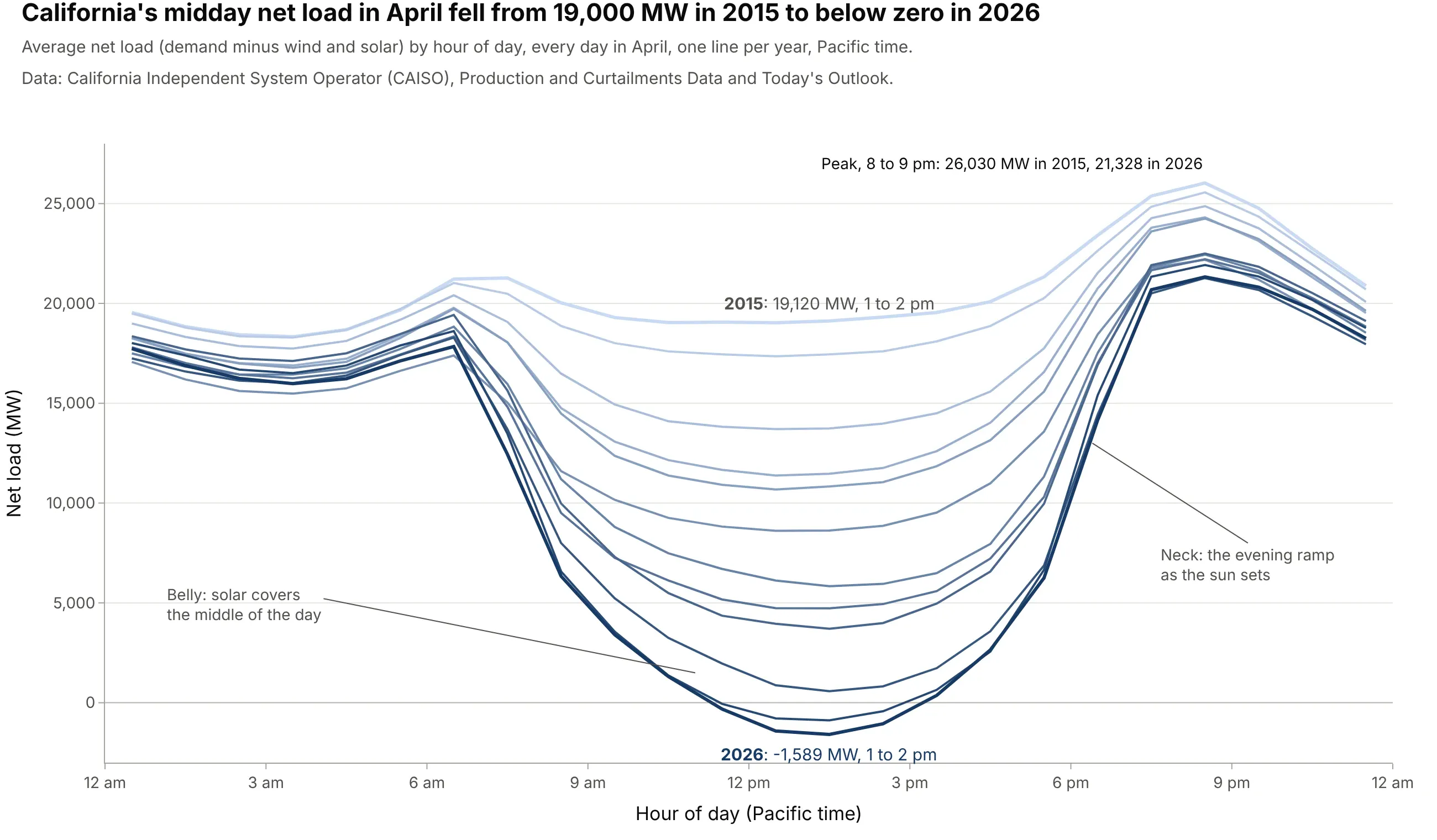
Data: California Independent System Operator (CAISO), Production and Curtailments Data (2015 to 2018) and Today's Outlook (2019 on).

How do you read a duck curve? In the example above, notice these things:

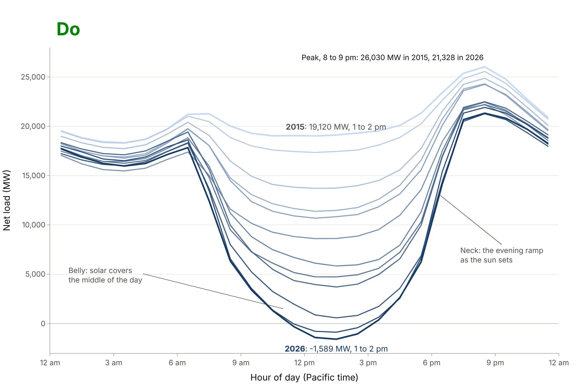
• The x axis is the hour of the day in local clock time (Pacific time, with daylight saving time in April), and each line is the average of the 30 days of April in one year. The y axis is net load in megawatts (MW): demand minus wind and solar generation, the part every other power plant, import and battery has to supply.
• The middle of the day is the belly. In 2015 it barely dipped; by 2026 the 1 to 2 pm average was -1,589 MW, below zero, because wind and solar produced more than California's customers used.
• The steep rise after 5 pm is the neck. The average 2026 day climbed 18,034 MW in three hours, against 5,291 MW in 2015, because solar disappears while people come home and demand peaks.
• The top of the neck, between 8 and 9 pm, fell from 26,030 MW in 2015 to 21,328 MW in 2026, so the problem got harder at both ends: a deeper belly and a sharper climb to almost the same evening peak.

It's often used for charts like these:

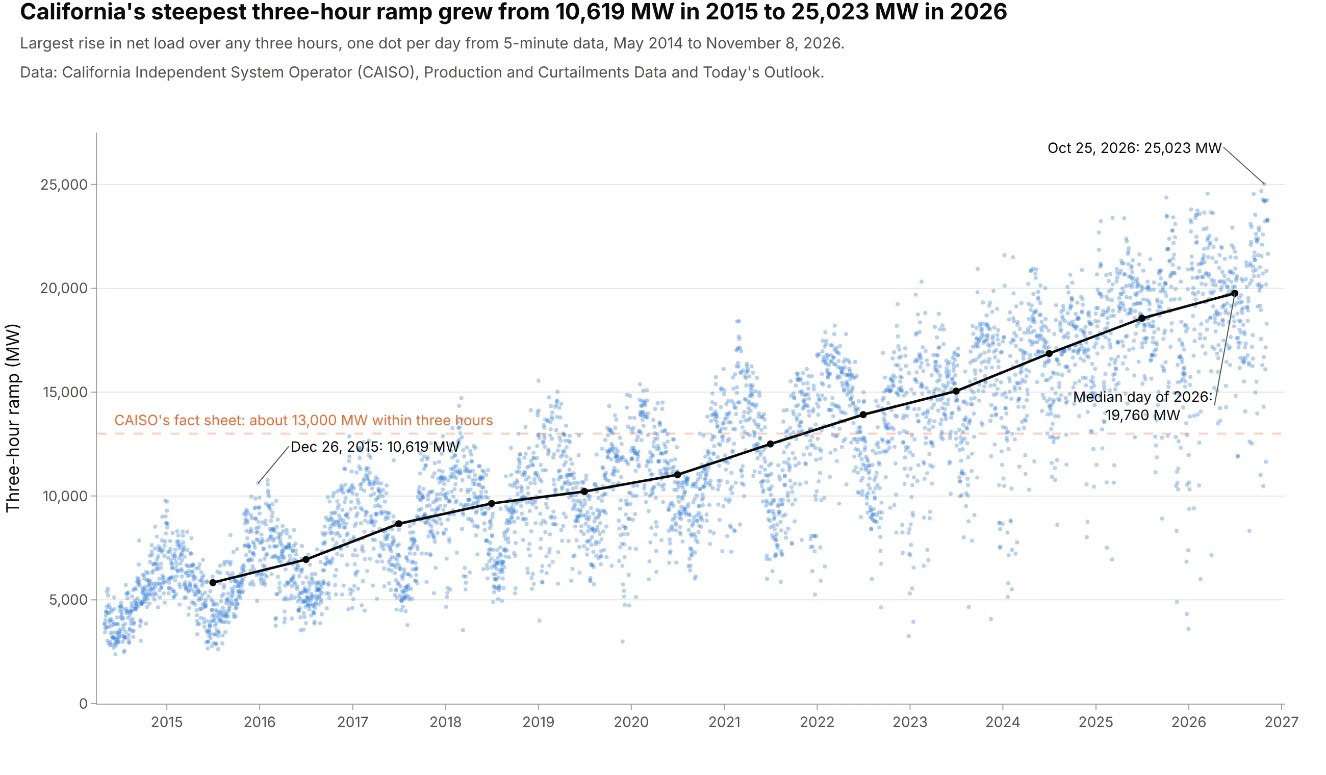
Planning for the evening ramp, the classic use. CAISO's duck chart warned of a need for about 13,000 MW within three hours; the first day past it came in January 2018, and the median day of 2026 needed 19,760 MW. Data: CAISO, Production and Curtailments Data and Today's Outlook.

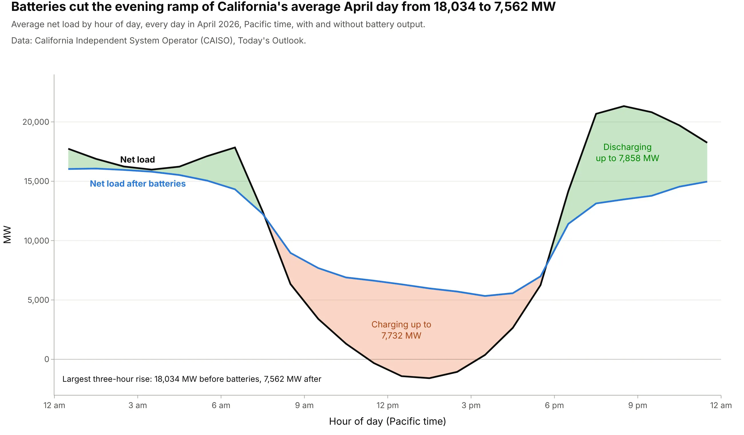
Seeing what batteries do. Subtracting battery output from net load and filling the space between the lines shows the energy moving from the belly to the neck: it cut the April 2026 evening ramp from 18,034 to 7,562 MW. Data: CAISO, Today's Outlook.

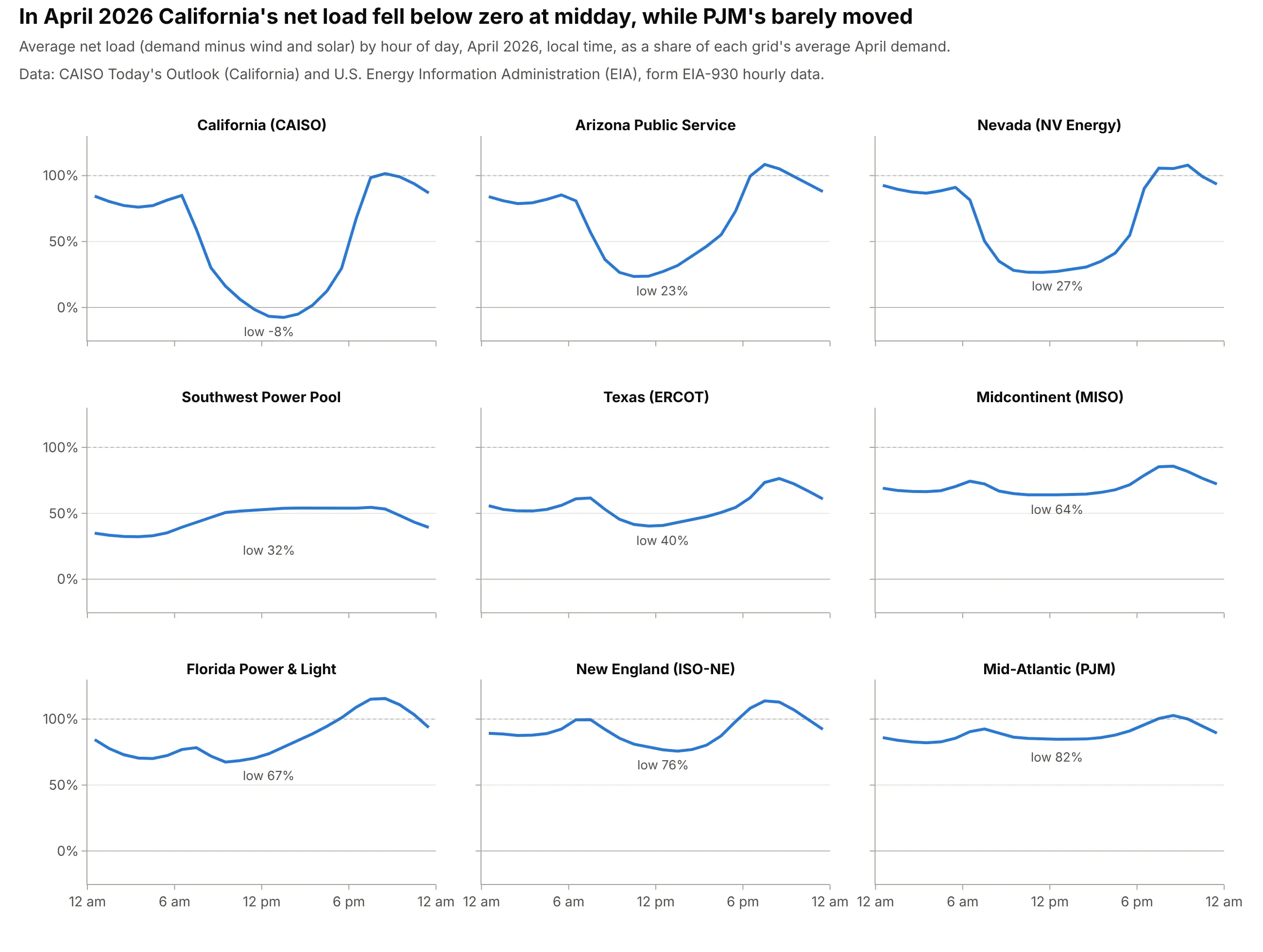
Comparing grids with small multiples. Dividing by each grid's average demand puts nine US grids on one scale: California's midday net load fell to -8% of its average demand in April 2026, PJM's stayed above 82%. Data: CAISO, Today's Outlook, and the U.S. Energy Information Administration (EIA), form EIA-930 hourly data.

A short history

In late 2012 CAISO published a study of how California's grid would run as it moved toward 33% renewable power by 2020, and one chart from it, net load on March 31 for every year from 2012 to 2020, became famous for its shape (RMI 2013, Inside Energy 2014). The lines for 2012 and 2013 were measured and the rest projected, with the midday low sinking each year toward about 12,000 MW in 2020. CAISO's fact sheet What the duck curve tells us about managing a green grid explains the name: the curves "produce a 'belly' appearance in the mid-afternoon that quickly ramps up to produce an 'arch' similar to the neck of a duck", which gave them "the industry moniker of 'The Duck Chart'". In Hawaii, Hawaiian Electric's planners described the shape on their island grids as "what has been coined the 'Nessie curve,' which is similar to California's 'duck curve'" (Nakafuji 2016). Here is CAISO's chart redrawn with what actually happened on March 31 in the years its 5-minute data covers:

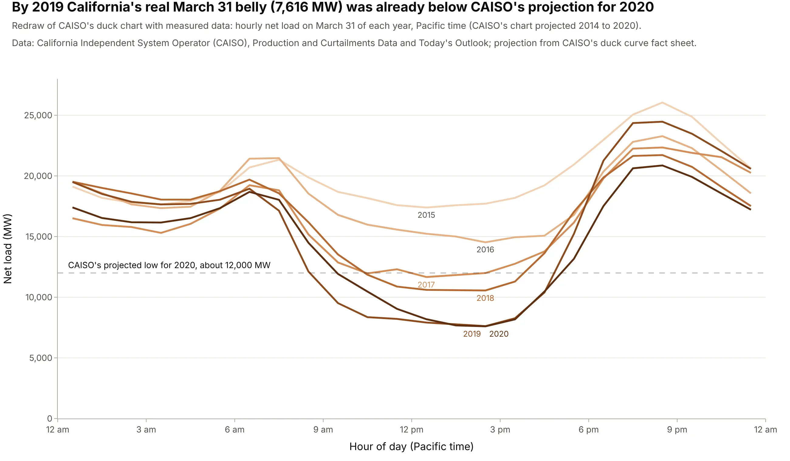
Data: CAISO, Production and Curtailments Data and Today's Outlook; the projected 2020 low is read from CAISO's fact sheet. By 2019 the real belly, 7,616 MW, was already well below CAISO's projection for 2020, and in April 2025 the monthly average went below zero.

How a duck curve works

A duck curve is a summary of how a power grid balances supply and demand hour by hour. These are the ideas it assumes, in the order a grid operator thinks about them.

Net load: the part of demand someone has to dispatch

A grid operator has to match generation to demand every second, and it can't tell the sun or the wind what to do. So it subtracts the wind and solar output it expects from the demand it expects, and what's left, the net load, is what it must cover by turning other resources up or down: gas plants, hydropower, imports from neighboring grids and batteries. CAISO's fact sheet calls net load "the variable portion that ISO must meet in real time". Here is one April day, with the wind and solar shaded between demand and net load:

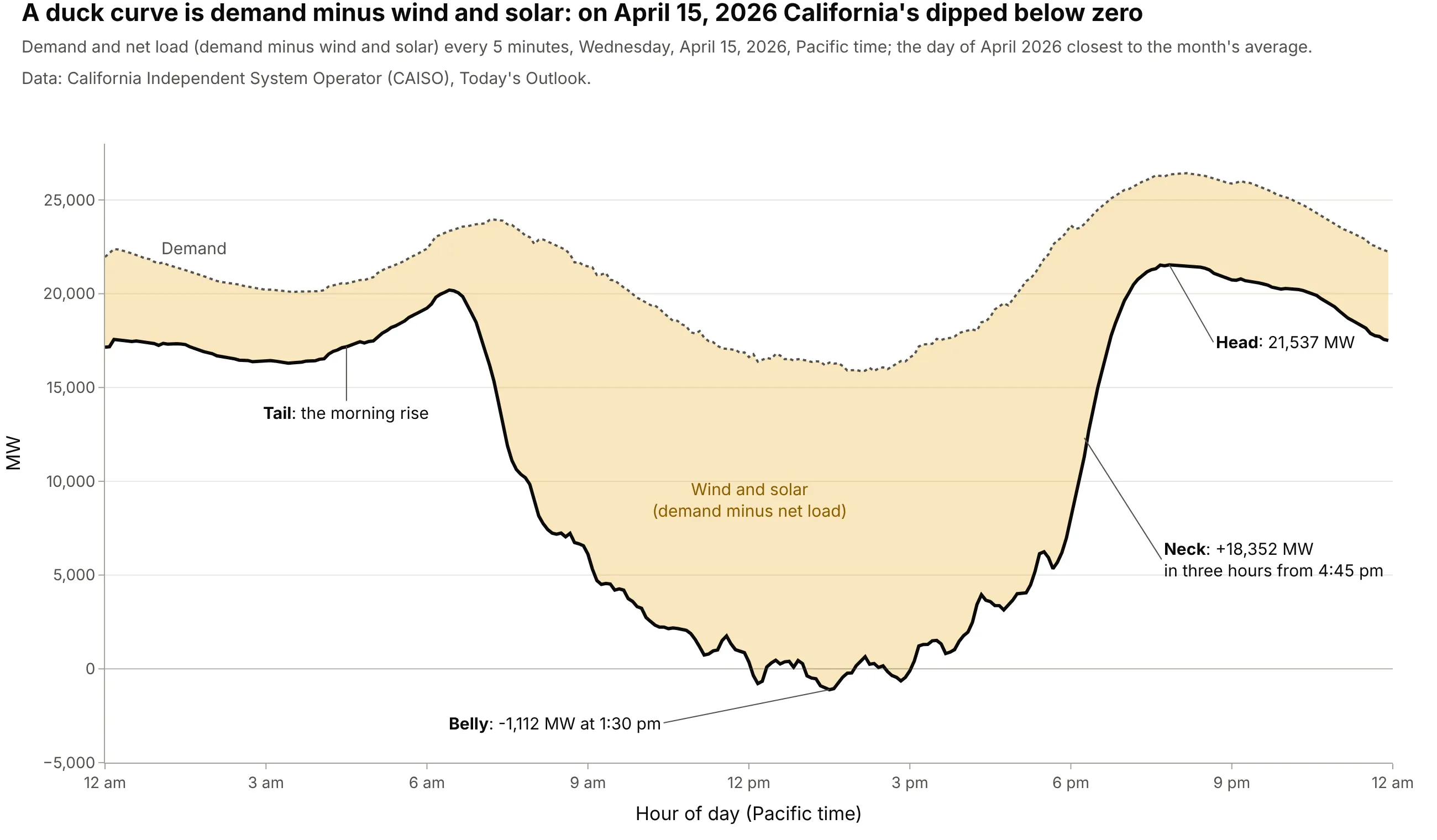
Data: CAISO, Today's Outlook. This is the day of April 2026 closest to the month's average.

CAISO's fact sheet names the parts: the morning rise is the duck's tail, the midday low the belly, and the evening climb the neck. Notice that demand itself dips at midday too. Part of that is rooftop solar: panels behind customers' meters aren't in the operator's solar figures, so they show up as lower demand.

Hours, time zones and averages

Grid data comes in intervals, and the convention matters. CAISO publishes 5-minute values in Pacific clock time; EIA's EIA-930 data, which covers every US balancing authority (the organization that balances supply and demand in one area), is hourly and labels each hour by its end, so "hour 14" is 1 to 2 pm. This guide averages each hour and plots it at the middle of the hour. Always plot in local time: in Coordinated Universal Time (UTC) the belly lands in the evening (see the dos and don'ts below). And remember that a duck curve is usually an average of many days, which hides the spread between sunny and cloudy days and weekdays and weekends (example 3 below).

The belly: oversupply and curtailment

When the belly gets deep enough, wind and solar can produce more than the grid can use, store or export. The operator then curtails, telling solar and wind plants to produce less than they could, and the energy is lost. CAISO's fact sheet called this "oversupply" and expected it "during the middle of the day". California's curtailment grew from 188 gigawatt-hours (GWh) in 2015 to 3,766 GWh in 2025:

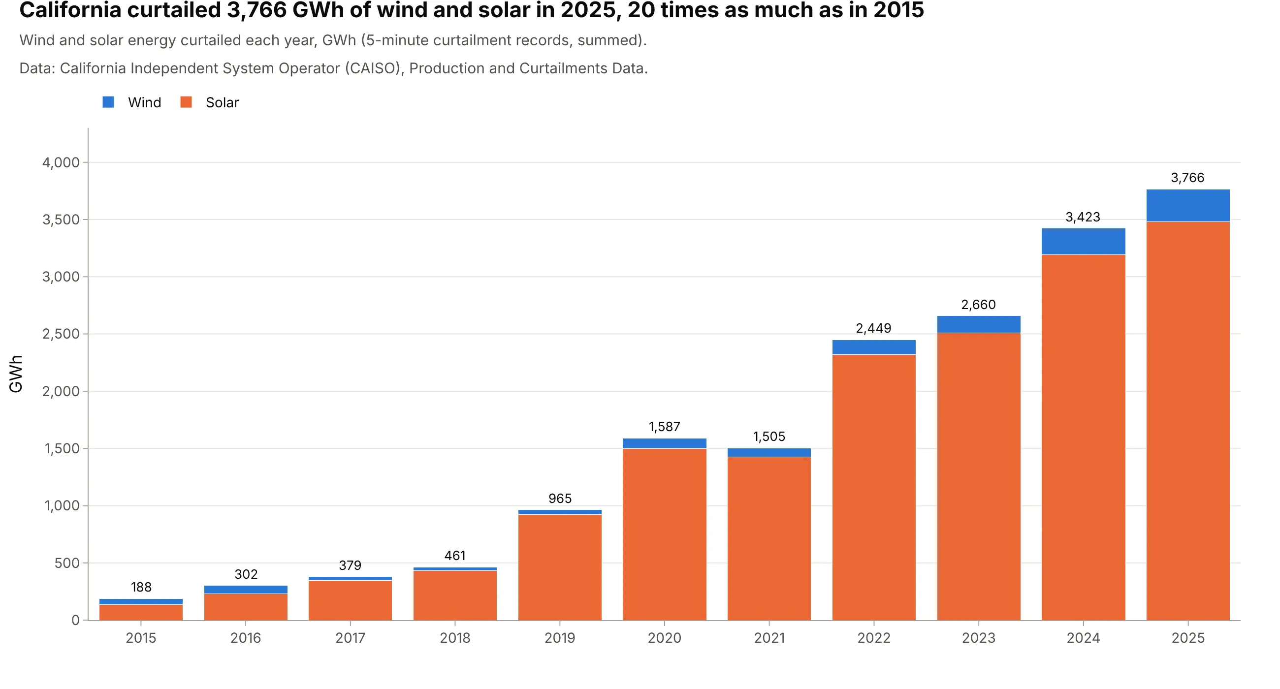
Data: CAISO, Production and Curtailments Data. Example 4 below shows when in the day and year it happens.

The neck: ramping

The neck is the ramp: how fast other resources have to come up as solar goes away. Grid planners measure it as the largest rise in net load over one or three hours, because power plants can only change their output so fast, and some take hours to start. CAISO's fact sheet warned of "an additional 13,000 MW, all within approximately three hours"; the steepest day of 2026 so far needed 25,023 MW (the ramp chart above).

Batteries flatten the duck

Batteries change the shape because they can be load and supply in the same day. They charge in the belly, which raises the net load the rest of the fleet sees, and discharge in the neck, which lowers it. That's why grid analysts now draw net load twice, before and after batteries, as in the chart above, and why the EIA wrote in 2023 that storing midday solar "flattens the duck's curve" and using it in the evening "shortens the duck's neck" (EIA 2023).

Alternatives to a duck curve

Here's the same month of California grid data drawn six ways. Some are better for the question, some worse, some just different:

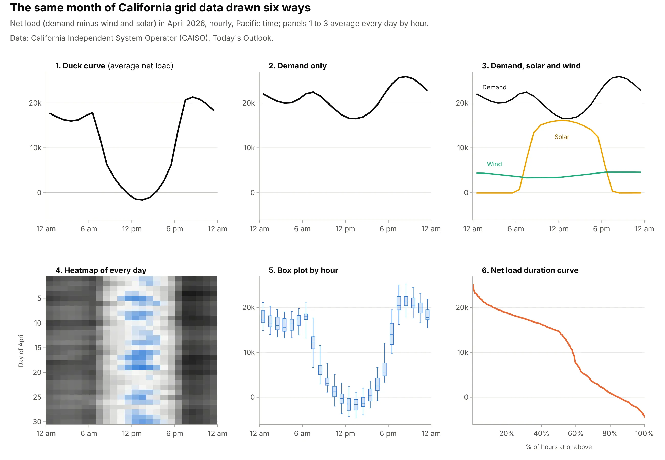
• Demand alone (worse). It dips only gently at midday, because most solar is subtracted later, so it hides the belly and the ramp, which are what the operator has to plan for.
• Demand, solar and wind as separate lines (works too). Every number is there, but the reader has to subtract in their head; an area chart of generation by source has the same problem.
• Heatmap of every day by hour (better for a whole month or year). Each row is one day, so cloudy days and weekends show up instead of being averaged away. Calendar heatmaps work the same way.
• Box plot by hour (works too). It keeps the average day's shape and adds the spread, which matters for planning reserves.
• Net load duration curve (different). Sorting every hour from highest to lowest loses the time of day but shows how many hours need how much capacity, which planners use to size power plants. It's closely related to an ECDF plot.

How to make a duck curve

With AI

ChatGPT, Claude Code, GitHub Copilot, Cursor and other AI tools are excellent at writing Plotly code. Name Plotly in the prompt, and say which days to average, which time zone to use, and how to color the years:

With Plotly Studio

Plotly Studio is a desktop app where you point an AI at a dataset and it builds charts and a Dash app around your questions. Ask for a duck curve the same way:

Show a duck curve of average net load (demand minus solar and wind) by hour of day for the selected month, one line per year in shades of blue, with a dropdown to pick the month and a toggle to subtract battery output.

Make a duck curve in Python or JavaScript

This is the code AI tools write under the hood. A duck curve is an ordinary Plotly line chart: compute net load, average it by hour of day, and draw one line per year with px.line:

For small multiples of several grids, add a grid column and use px.line(..., facet_col="grid", facet_col_wrap=3). To fill between net load and net load after batteries, draw the second line as a go.Scatter with fill="tonexty" right after the first.

In JavaScript, plotly.js draws the same chart from the hourly averages:

Share it

Every Plotly chart has a Share chart button (the cloud icon in its toolbar) that uploads it to Plotly Cloud and gives you a link. Only you can see it until you change its visibility.

For a live app, put the chart in a Dash app and publish it with the Plotly Cloud command-line interface (CLI). Coding agents can run these commands for you:

If your data has to stay in your own cloud or data center, publish to Dash Enterprise instead.

Dos and don'ts

Most of the mistakes in a duck curve are about time and order: which clock the hours are on, and whether the colors show that the years follow each other. Here is the main example both ways.

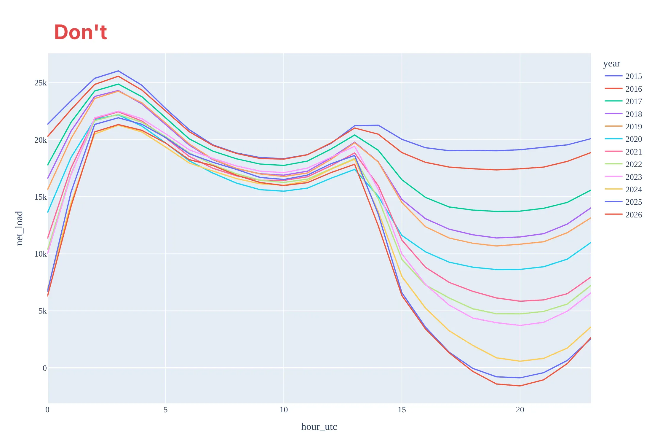
Don't plot the hours in UTC, which moves the belly to the evening and the peak to the early morning, give 12 ordered years 12 unrelated default colors with a 12-entry legend, or keep raw column names, no units and a serif font:

Do plot local clock time and say which zone in the axis title, use one hue from light to dark so the years read in order, label the first and last years on the chart, put the units on the axis and mark zero:

Checklist

Do

• Use local clock time, say which zone, and say whether hours are labeled by their start or their end.
• Say which days were averaged (a month, a season, weekdays only) and how many.
• Use a sequential palette for years and a categorical one only for unrelated groups such as grids.
• Draw a zero line once net load can go negative, and give MW or gigawatts (GW, 1,000 MW) in the axis title.
• Divide by average demand when you compare grids of different size.

Don't

• Mix the operator's own net load with one you computed without saying so; they can differ (see the FAQ).
• Compare a single day from different years as if it were a trend: California's March 31, 2026 low (11,590 MW) was about the same as 2017's (11,666 MW).
• Stack wind and solar on top of demand in an area chart and call it a duck curve; the duck is the line that's left.
• Use a dual y axis for demand and net load; they share units and belong on one axis.

Options to customize

A duck curve in Plotly is a line chart of hourly averages, so these are the options that matter most. The full lists are in the px.line reference, the scatter trace reference and the filled area documentation.

1. px.line(df, x="hour", y="net_load", color="year"): one line per year or season from a long table.
2. color_discrete_sequence=px.colors.sequential.Blues[1:]: a light-to-dark palette so years read in order.
3. category_orders={"year": [...]}: keeps the years, months or grids in the order you want.
4. fig.update_xaxes(tickvals=..., ticktext=["12 am", "3 am", ...]): clock labels instead of 0 to 23.
5. fig.add_hline(y=0): the zero line, which matters once the belly goes negative.
6. fill="tonexty" on a go.Scatter: shades between two lines, such as net load before and after batteries or demand and net load.
7. facet_col="grid", facet_col_wrap=3: small multiples of several grids or months on shared axes.
8. fig.add_annotation(...): direct labels for the first and last years, the low and the peak, instead of a legend.
9. go.Heatmap(z=..., x=hours, y=days): every day of a year by hour, when the average hides too much.
10. go.Scattergl: years of 5-minute data as one WebGL trace (see the FAQ).

More duck curve examples

Seven more duck curves and related grid charts built from real public data, each with its source, the technique that makes it work, and a prompt to rebuild it.

1. Texas: ERCOT's duck is forming

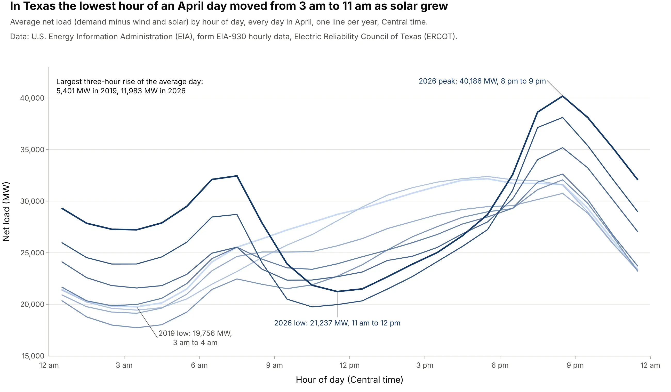
The Electric Reliability Council of Texas (ERCOT) used to have its lowest net load in the middle of the night, when the wind blows hardest. As its solar grew, the low moved to late morning, and the largest three-hour rise of the average April day more than doubled, from 5,401 MW in 2019 to 11,983 MW in 2026. Data: EIA, form EIA-930 hourly data.

Tip: use the same palette and axes as your California chart, so readers can compare shapes across grids at a glance.

2. Seasons: April's belly, August's neck

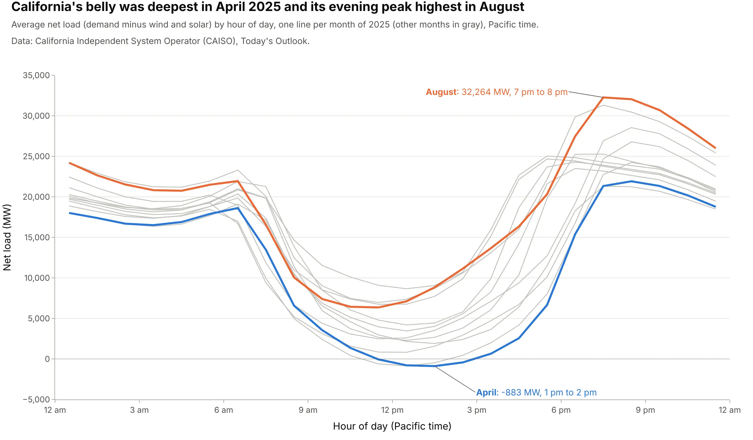
Spring brings strong sun and mild weather, so April 2025 had California's deepest belly, -883 MW from 1 to 2 pm, while summer air conditioning made August's evening peak the highest at 32,264 MW. Operators plan for both: oversupply in spring and the steepest climb to the highest peak in late summer. Data: CAISO, Today's Outlook.

Tip: highlight the two months that answer the question and gray out the rest instead of using 12 colors.

Another way to see it: a heatmap with one row per day keeps the weather and weekends that the monthly averages smooth out. Hourly net load fell below zero on 96 days of 2025, 71 of them from March to June:

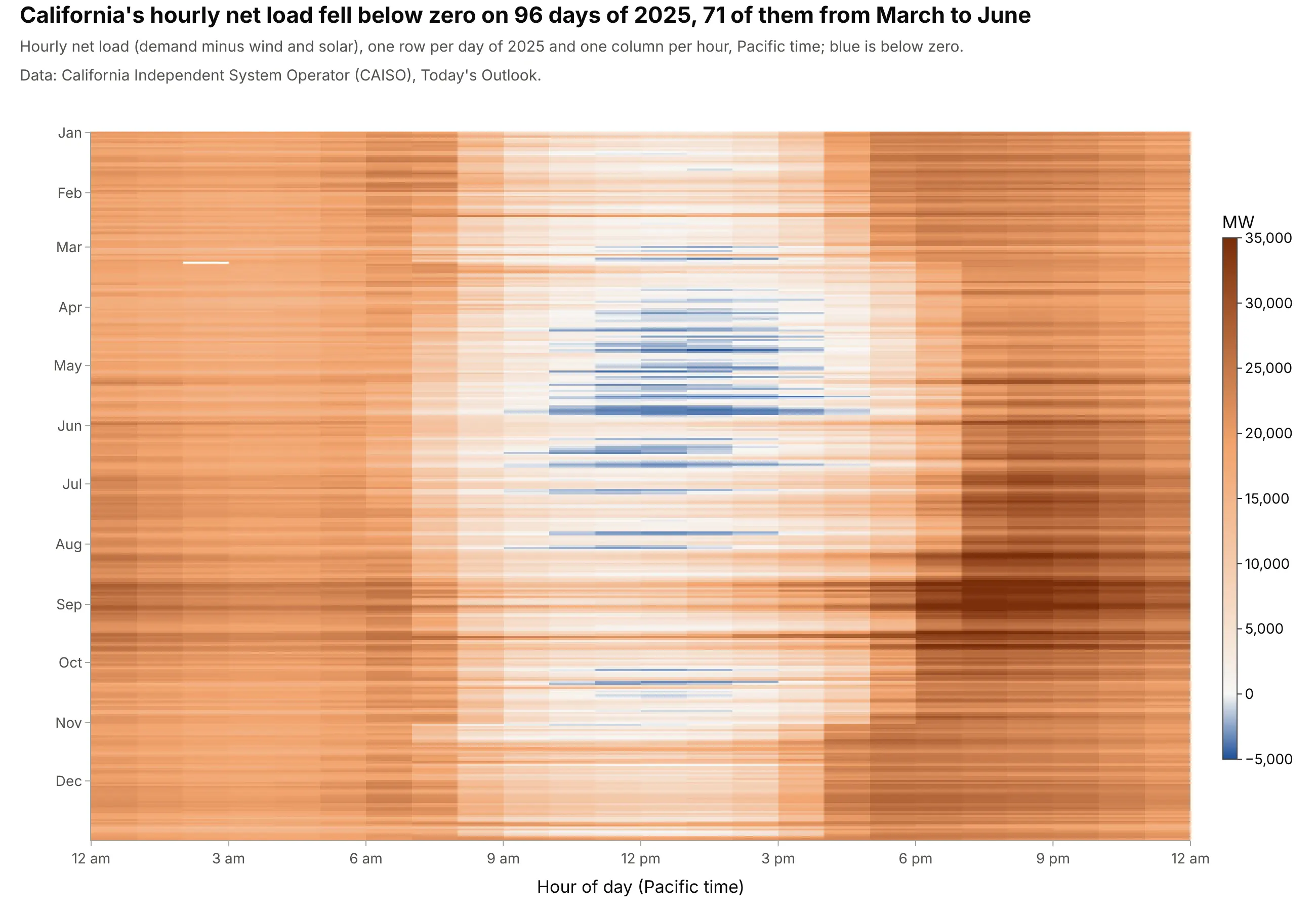
3. Every day of April 2026, not just the average

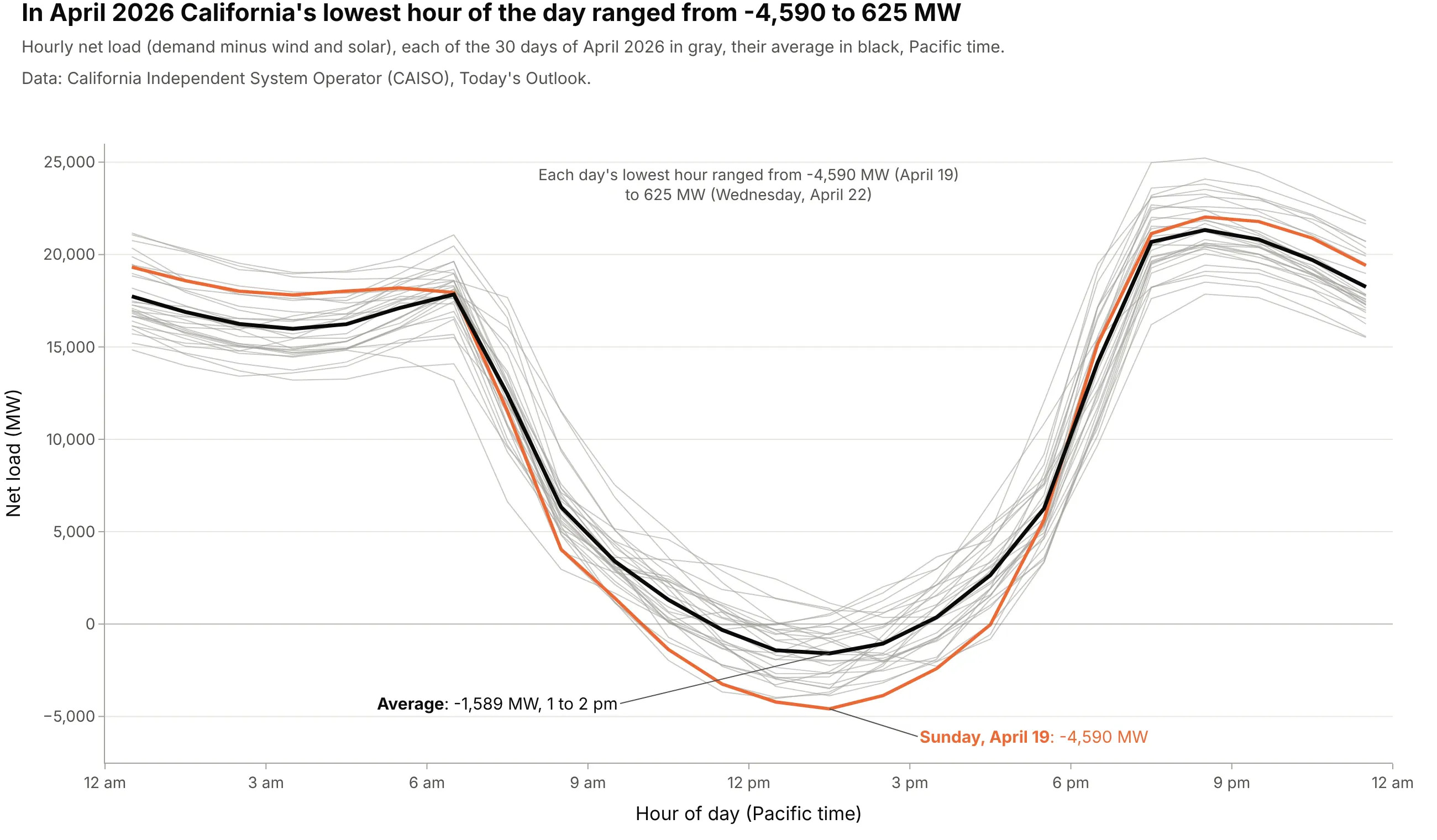
The average April 2026 day bottomed at -1,589 MW, but single days ranged from -4,590 MW (Sunday, April 19) to 625 MW (Wednesday, April 22). Weekends have less demand and cloudy days less solar, and grid operators have to plan for the extremes, not the mean. Data: CAISO, Today's Outlook.

Tip: draw every day as a thin gray line behind the average, then color only the day you want to talk about.

4. Curtailment lives in the belly

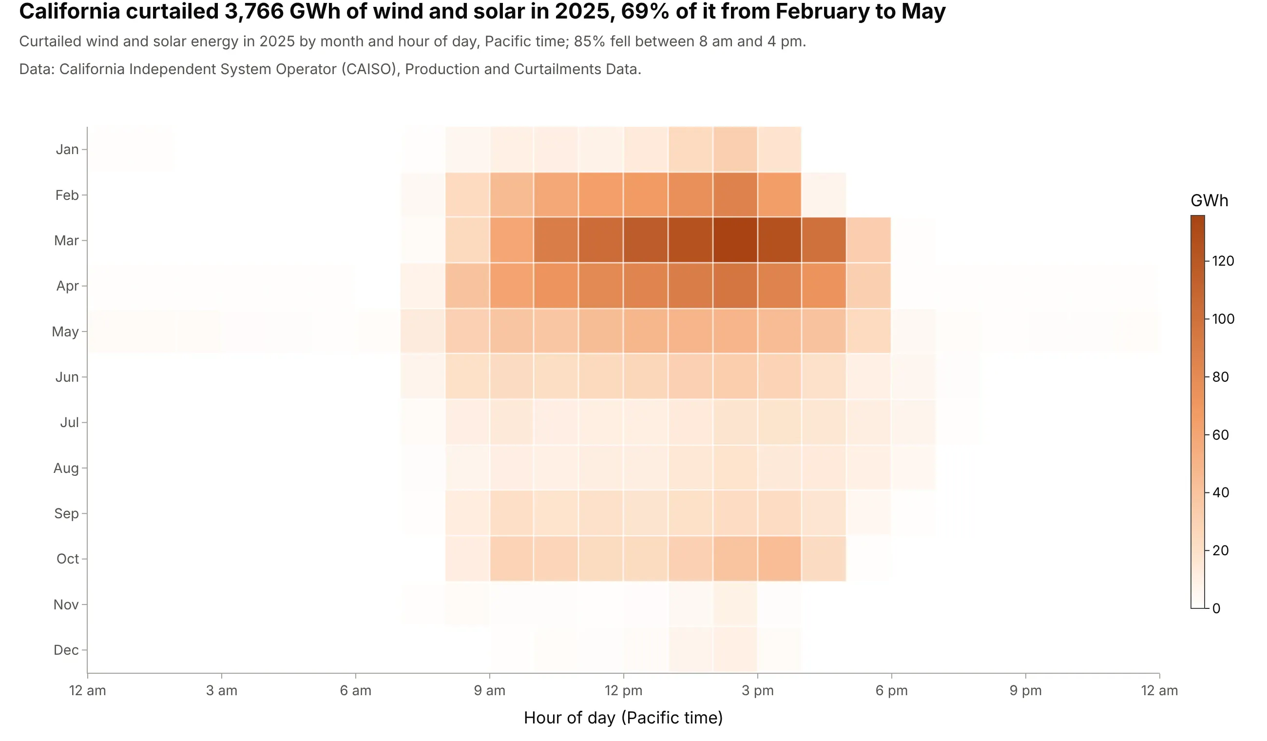
California curtailed 3,766 GWh of wind and solar in 2025, 92% of it solar. 85% fell between 8 am and 4 pm and 69% between February and May, the same hours and months as the deepest belly. Data: CAISO, Production and Curtailments Data.

Tip: put hours on the x axis exactly as in your duck curves, so the heatmap reads as the belly seen from above.

5. Below zero: the lowest net load of every day

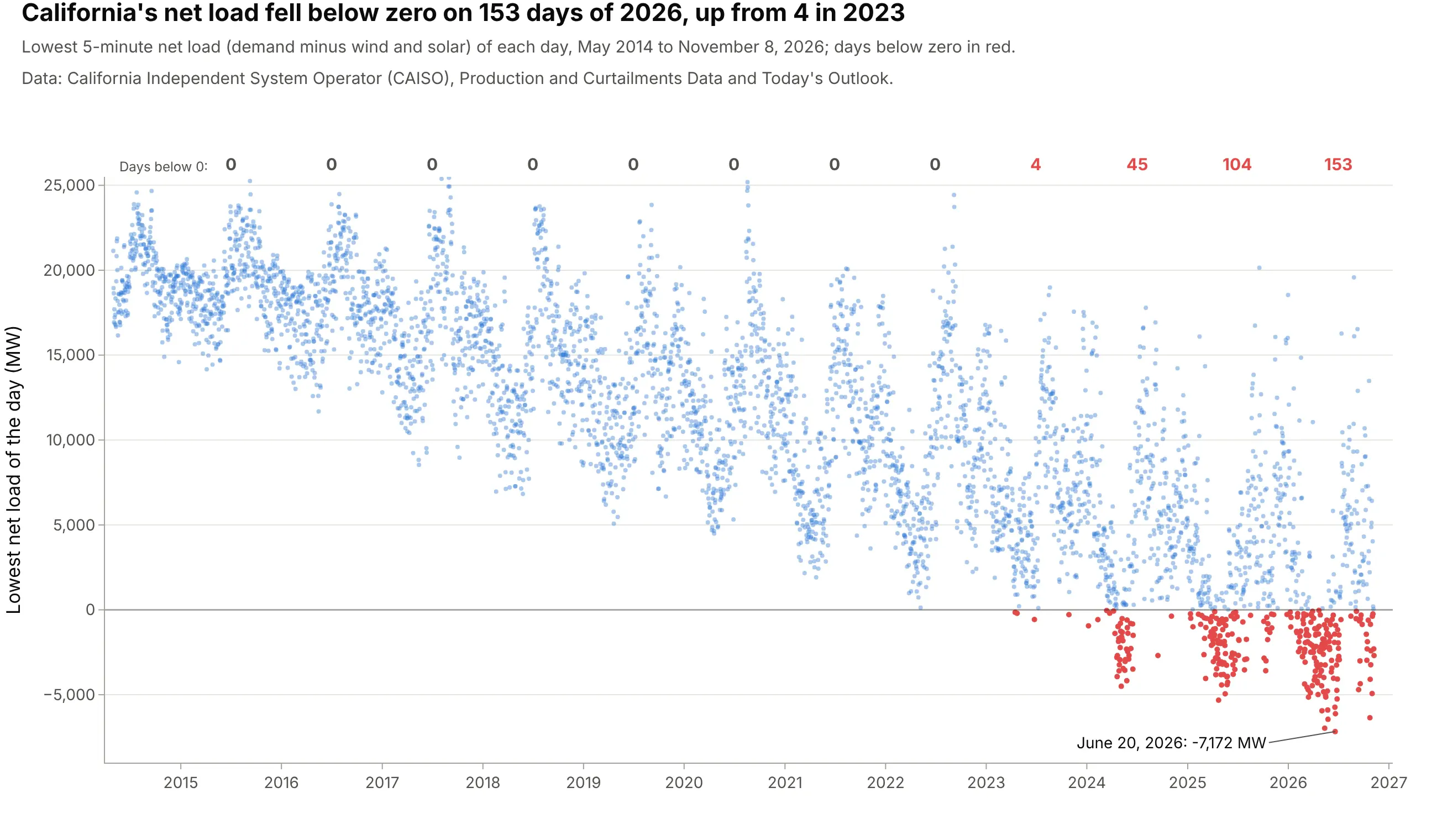
California's net load first fell below zero on 4 days of 2023; in 2026 it did so on 153 days by November 8, with a low of -7,172 MW on June 20. When net load is negative, wind and solar alone exceed what the area's customers use, and the rest is stored, exported or curtailed. Data: CAISO, Production and Curtailments Data and Today's Outlook.

Tip: count the days past a threshold and write the counts above each year, so the trend doesn't depend on reading dots.

6. California's batteries mirror the duck

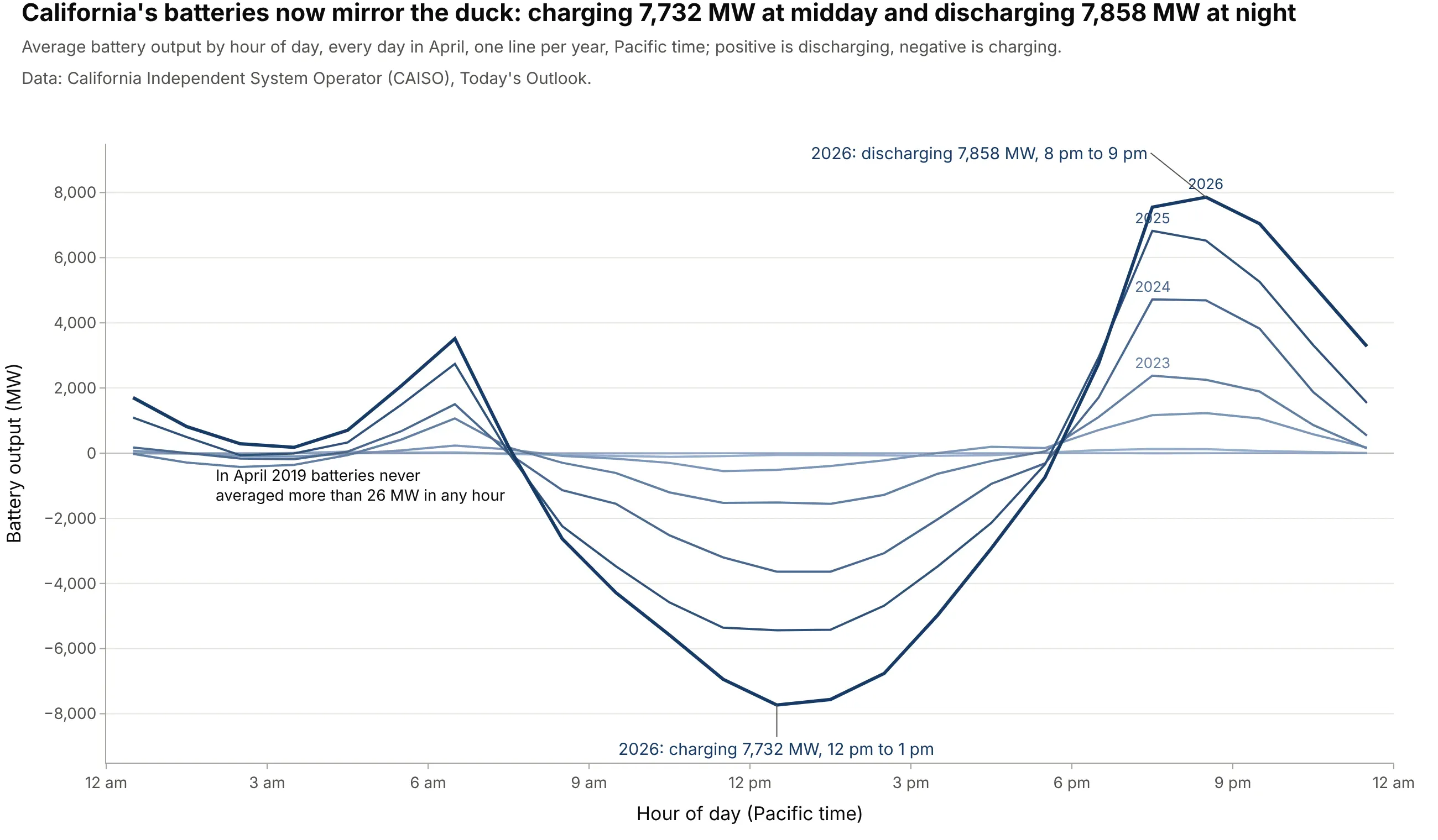
In April 2019 California's batteries never averaged more than 26 MW in any hour. By April 2026 they charged 7,732 MW in the 12 pm hour and discharged 7,858 MW from 8 to 9 pm, the duck turned upside down. Data: CAISO, Today's Outlook (supply by source).

Tip: keep the same hour axis and year palette as your duck curve, and draw a zero line so charging and discharging separate.

7. A measured signal: the October 2023 eclipse

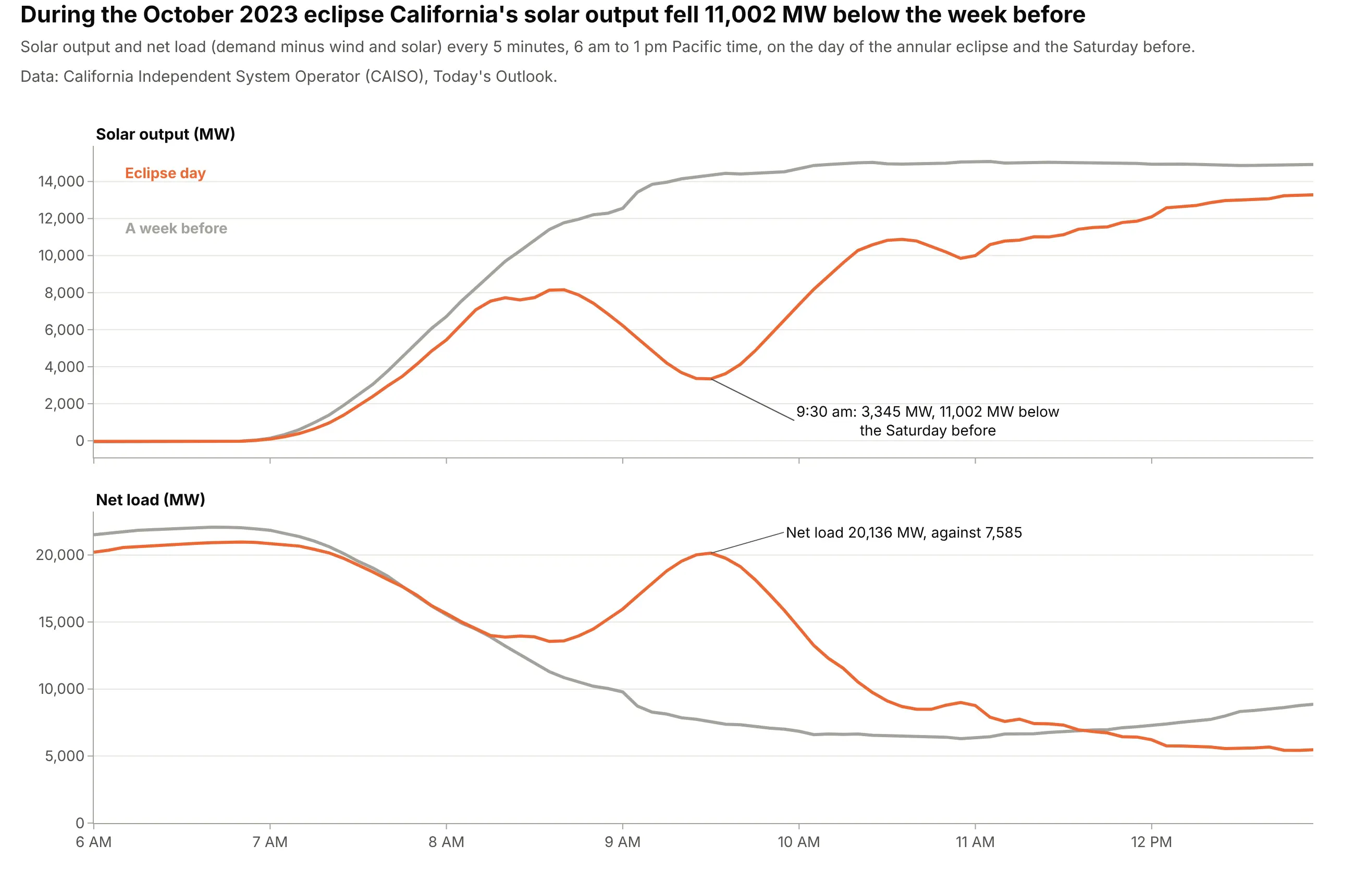
The annular solar eclipse of October 14, 2023 dimmed the sun over California for about an hour. At 9:30 am solar output was 3,345 MW, 11,002 MW below the Saturday before, and net load rose to 20,136 MW against 7,585: a small duck neck in the middle of the morning, which CAISO had to cover with other resources. Data: CAISO, Today's Outlook.

Tip: compare against a similar day (same weekday, a week earlier) at full 5-minute resolution, since hourly averages would blur the dip.