Calendar Heatmaps - A Complete Guide

TL;DR

• A calendar heatmap draws one colored cell per day, laid out like a wall calendar with weeks as columns, weekdays as rows and one block per year. GitHub's contribution chart is the best-known one.
• Calendar heatmaps are also known as calendar charts and calendar plots, and are similar to heatmaps and line charts of a daily series.
• Use one for a daily series over one to about eight years when the questions are about the calendar: which weekdays, which weeks, which holidays and which streaks.
• Use a line chart instead when the long-term trend or exact values matter more than the day-to-day pattern.
• You can make a calendar heatmap with Plotly from go.Heatmap on a week x weekday grid, one subplot per year. Any coding agent can write it for you, and this guide has a 30-line helper.

What is a calendar heatmap?

Calendar heatmaps look like this:

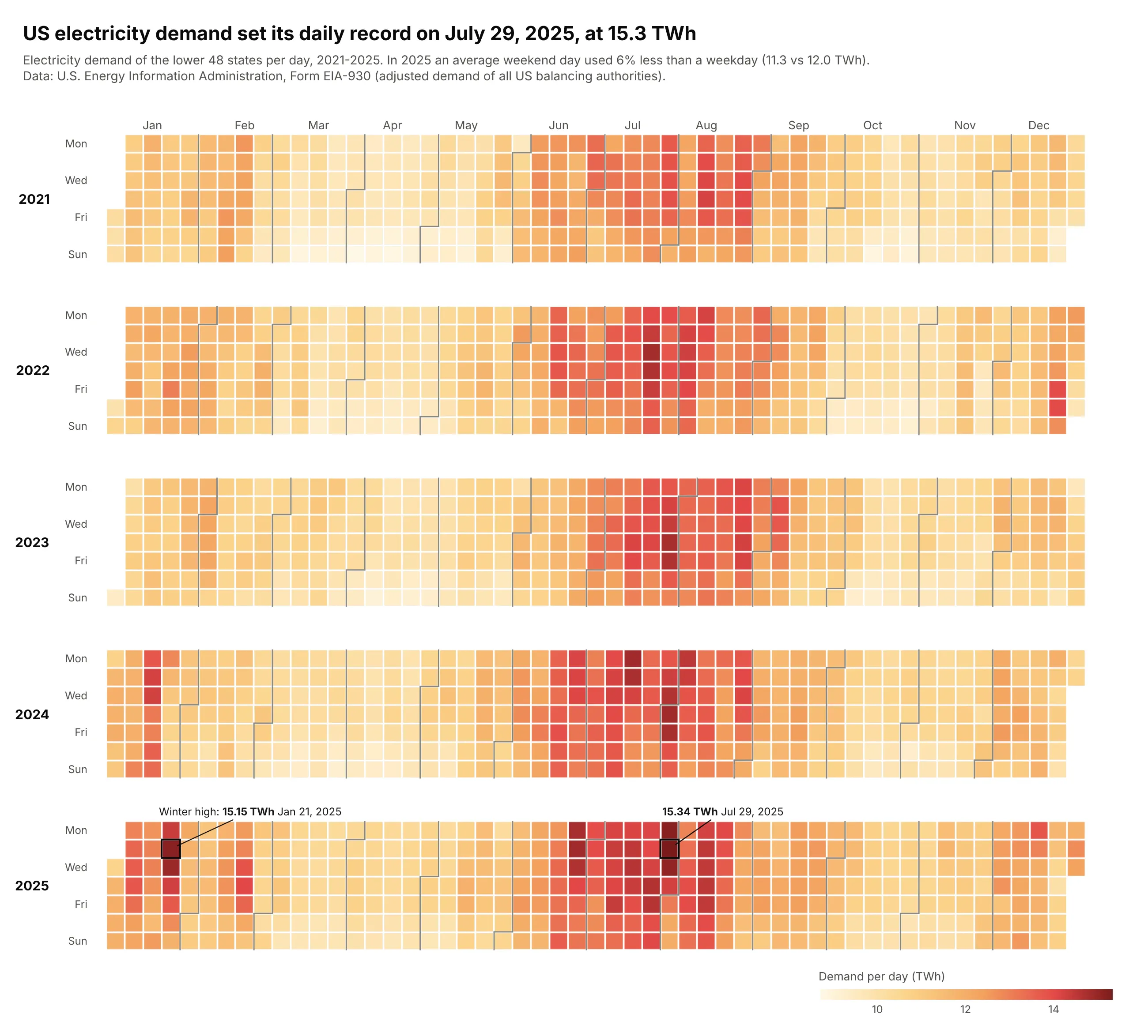
Data: U.S. EIA, Form EIA-930, 2021-2025.

How do you read a calendar heatmap? In the example above, notice these things:

• Each cell is one day of US electricity demand, colored from pale yellow on the quietest days to dark red on the busiest. Each year is one block, with weeks as columns and Monday to Sunday as rows, so a week reads from top to bottom.
• The gray step lines mark where each month begins. They zigzag because a month usually starts partway through a week, and the month labels along the top sit above them.
• Seasons show up as wide bands of color. In every year, June, July and August had the highest average demand, so each summer is a dark red band, and short dark columns in winter, like the one in January 2025, mark weeks of very high demand.
• Weekly patterns show up as rows. The bottom two rows of every block are lighter because an average weekend day in 2025 used 6% less electricity than a weekday.
• Color is good for spotting patterns and bad for reading exact values, so the record day and the winter high are labeled. The record on July 29, 2025 was only a little higher than the winter high in January, which you can only tell from the labels because both cells are at the dark end of the color scale.

It's often used for charts like these:

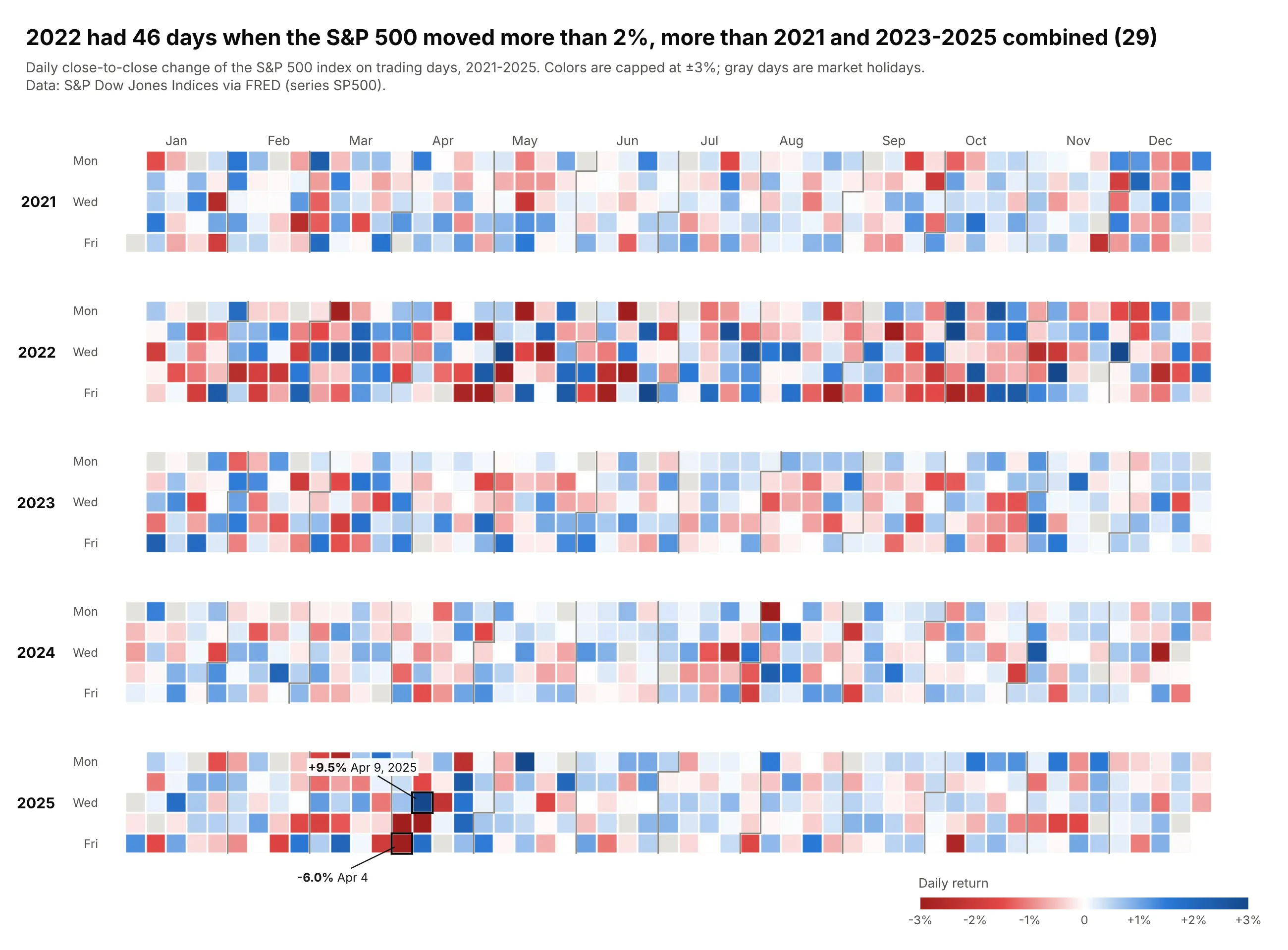
Daily market returns on a diverging scale. The S&P 500 moved more than 2% on 46 days in 2022, more than in 2021 and 2023-2025 combined (29), and its worst and best days of the five years, -6.0% and +9.5%, came five days apart in April 2025. Data: S&P Dow Jones Indices via FRED (SP500), 2021-2025.

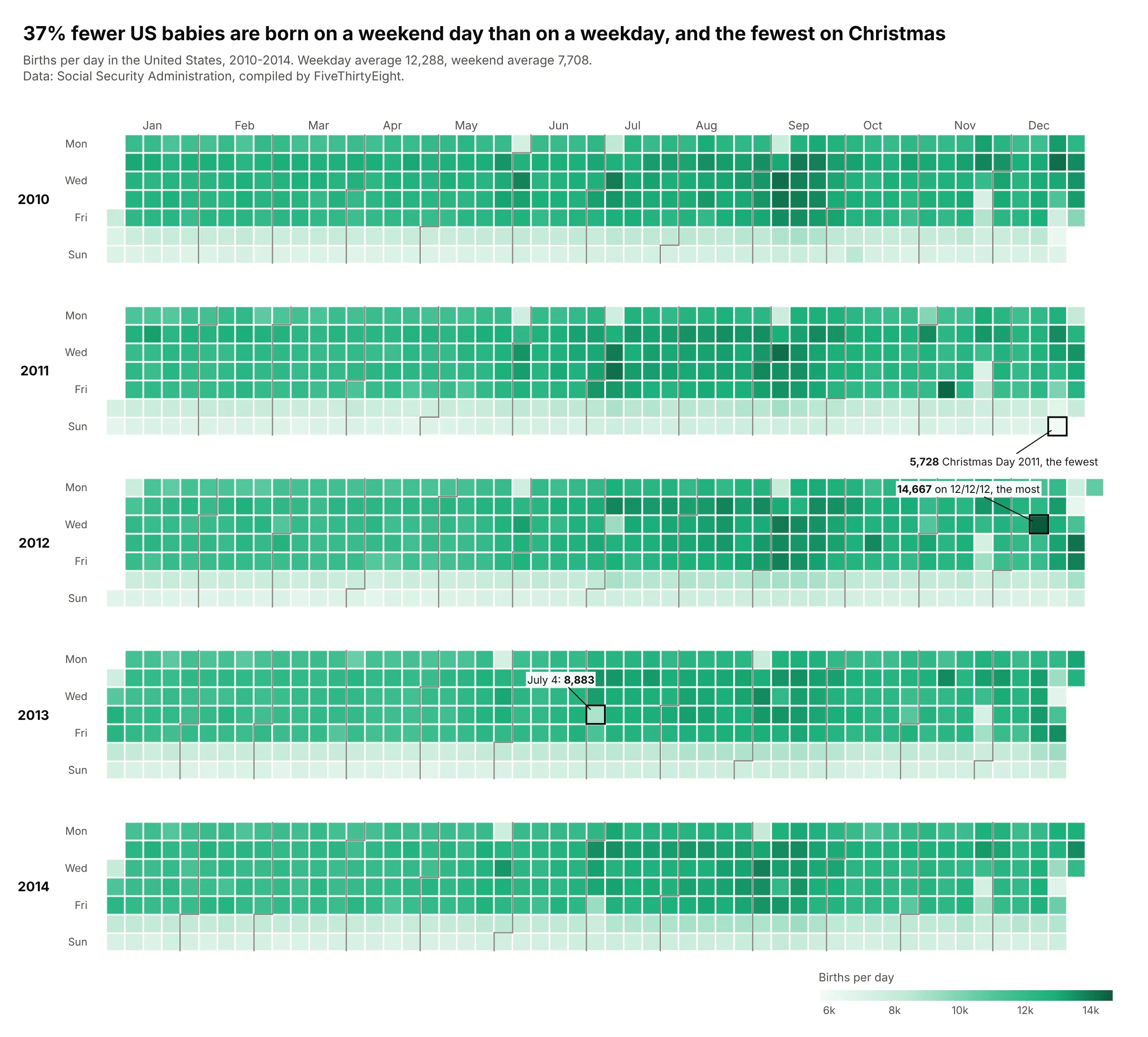
Health data with a weekly rhythm. About 37% fewer US babies are born on a weekend day than on a weekday (7,708 against 12,288 a day in 2010-2014), and holidays such as Christmas show up as pale cells inside dark weeks. Data: Social Security Administration via FiveThirtyEight, 2010-2014.

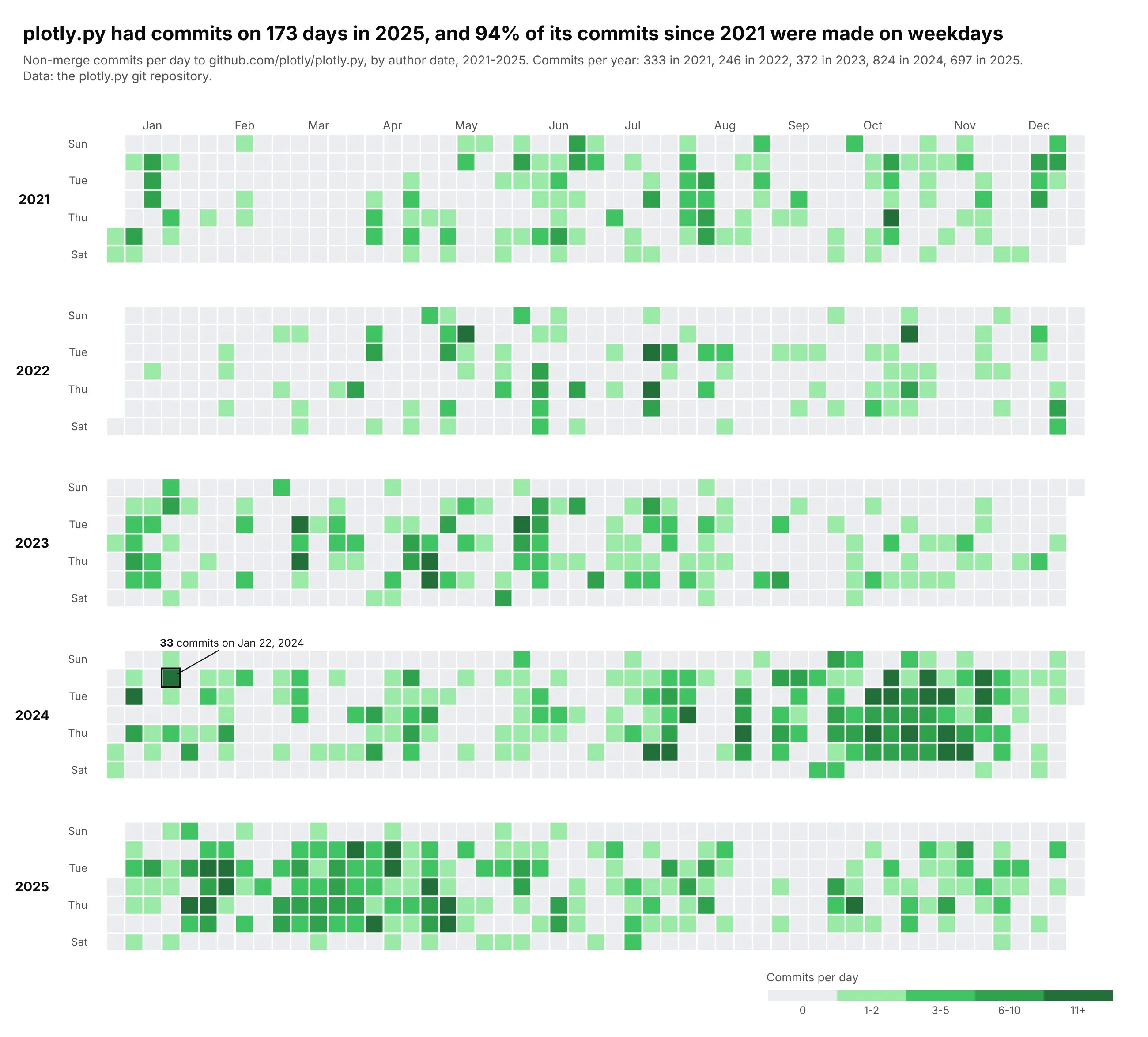
Activity, GitHub style. The plotly.py repository had commits on 173 days in 2025, and 94% of its commits since 2021 were made on weekdays, which is why its weekend rows are almost empty. Data: the plotly.py git repository, 2021-2025.

A short history

The calendar view comes from Jarke van Wijk and Edward van Selow's "Cluster and calendar based visualization of time series data" (IEEE InfoVis 1999, doi:10.1109/INFVIS.1999.801851). They grouped days with similar data into clusters (their examples were the number of employees present at a research institute and energy use) and colored each day of a calendar by its cluster, so that holidays and unusual days stood out. Here is that idea redrawn with Plotly on US births in 2014, which aren't their data but behave the same way: split into two clusters by births per day, every weekend day lands in one cluster and so do eight weekdays, all of them holidays or days next to one.

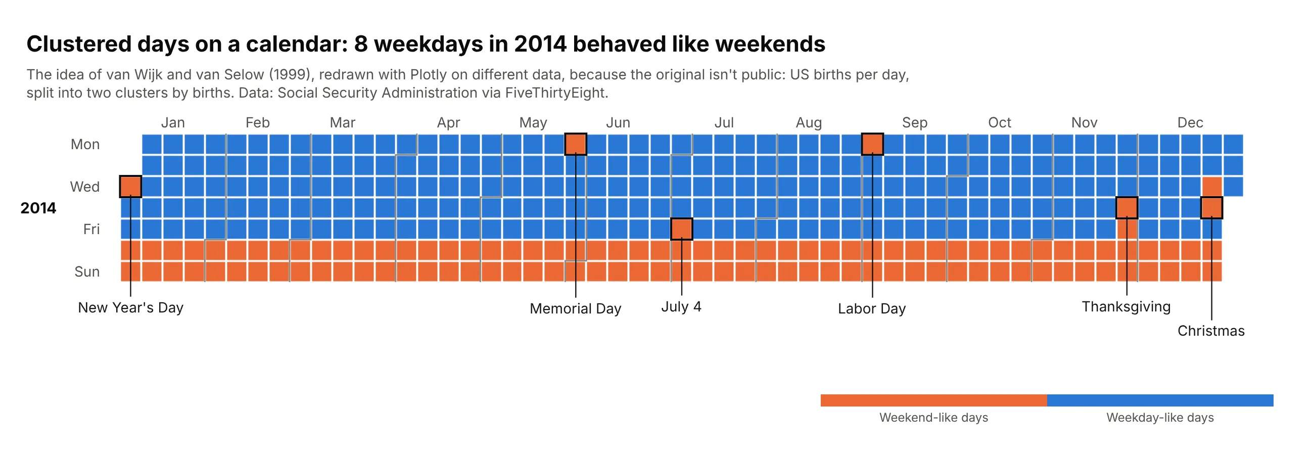
GitHub's contribution graph later made the layout familiar to every developer, which is why many people search for a "GitHub-style heatmap".

Alternatives to a calendar heatmap

Here's the same five years of US electricity demand from the top of this page drawn four more ways. Some are better for the question, some worse, some just different:

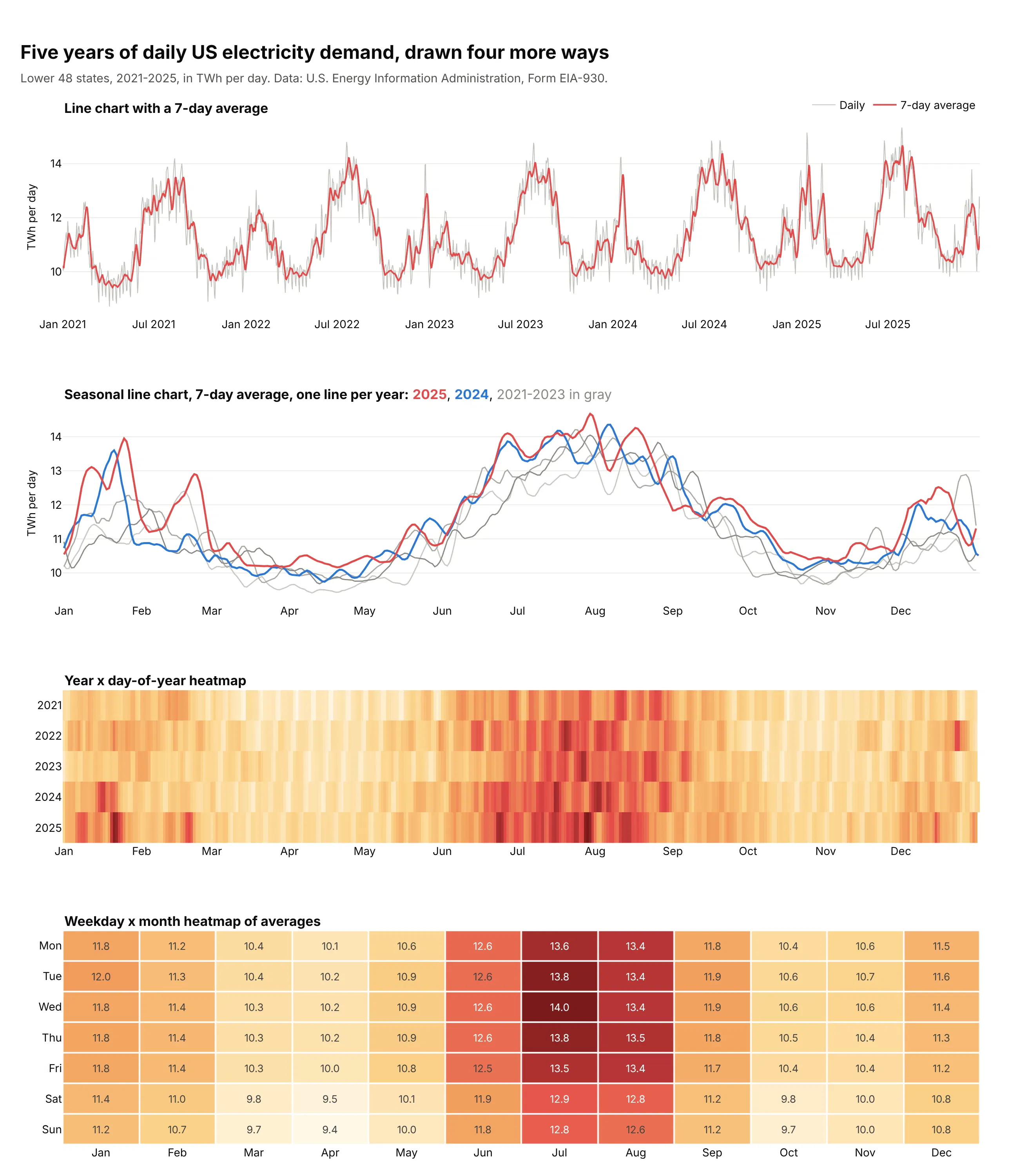
• Line chart with a 7-day average (better for the trend and exact values). People read position on a common scale more precisely than color, as Cleveland and McGill (1984) measured, so a line chart shows the summer and winter peaks and their exact levels best. The weekly rhythm turns into a gray zigzag, though, and you can't tell which day was a Sunday or a holiday.
• Seasonal line chart, one line per year (better for comparing years). Plotting each year against the day of the year shows that January 2025 averaged 12.7 TWh a day, the highest of the five Januaries (2021 averaged 11.0), but five overlapping lines get hard to read, and the weekdays are smoothed away.
• Year x day-of-year heatmap (works too, for many years). One thin row per year fits 20 or more years in a small space, so it's the better choice for long records. Weekdays don't line up between rows, so the weekly pattern turns into stripes. See our heatmap guide.
• Weekday x month heatmap of averages (different). Averaging days into a profile answers "when is demand high?" directly: July weekdays average 13.5 to 14.0 TWh and April weekends 9.4 to 9.5 TWh. It loses every individual day, so records and holidays disappear.

The calendar heatmap is the only one of these that keeps every day and its weekday, which is what you need when the question is about particular days.

How to make a calendar heatmap

With AI

ChatGPT, Claude Code, GitHub Copilot, Cursor and other AI tools are excellent at writing Plotly code. Name Plotly in the prompt, describe the grid and what the color should mean, and list the checks you want:

The last check matters because calendar heatmaps hide gaps well: a missing week looks like a quiet week unless missing days are drawn differently.

With Plotly Studio

Plotly Studio is a desktop app where you point an AI at a dataset and it builds charts and a Dash app around your questions. Ask for a calendar heatmap the same way:

Show a GitHub-style calendar heatmap of daily electricity demand: one row of weeks per year, weekdays from Monday to Sunday, month labels on top, gray for missing days and a yellow to dark red scale. Add a dropdown to switch to the change from the same day last year on a diverging scale centered on zero.

Make a calendar heatmap in Python or JavaScript

This is the code AI tools write under the hood. In Python, the function below turns any DataFrame with a date column and a value column into a calendar heatmap from go.Heatmap and make_subplots. It is a short version of the helper behind every example in this guide:

scaleanchor keeps the cells square, autorange="reversed" puts Monday on top, and the shared coloraxis gives every year the same scale. For a diverging series, pass zmid=0 (or your baseline) and a diverging colorscale such as "RdBu".

In JavaScript, plotly.js builds the same grid from one heatmap trace: compute each day's week column and weekday row, then pass them as x and y:

Share it

Every Plotly chart has a Share chart button (the cloud icon in its toolbar) that uploads it to Plotly Cloud and gives you a link. Only you can see it until you change its visibility.

For a live app, put the chart in a Dash app and publish it with the Plotly Cloud CLI. Coding agents can run these commands for you:

If your data has to stay in your own cloud or data center, publish to Dash Enterprise instead.

Dos and don'ts

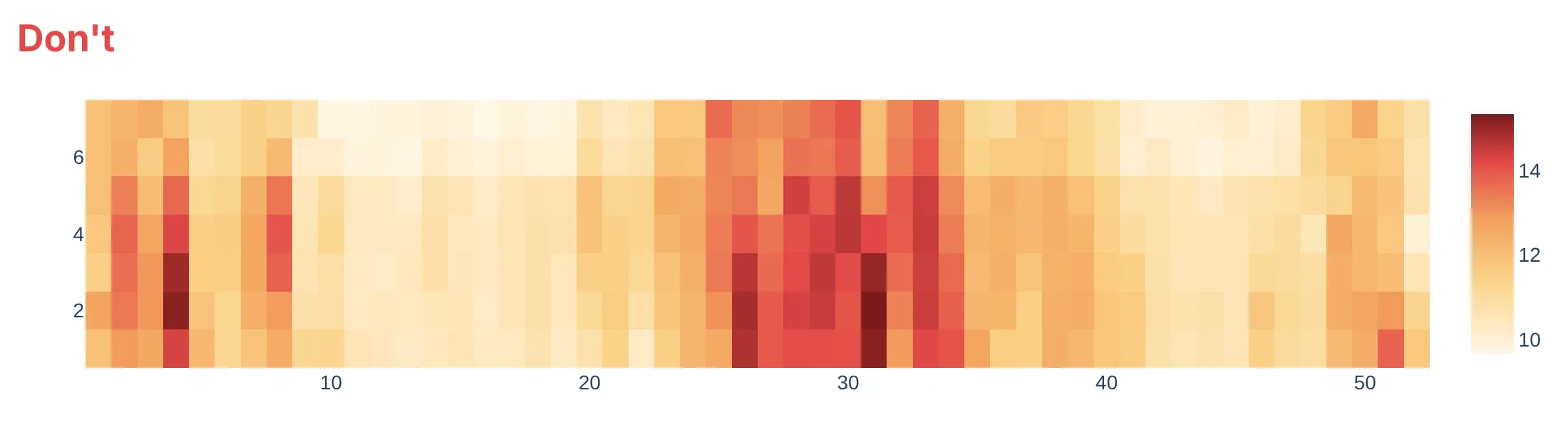
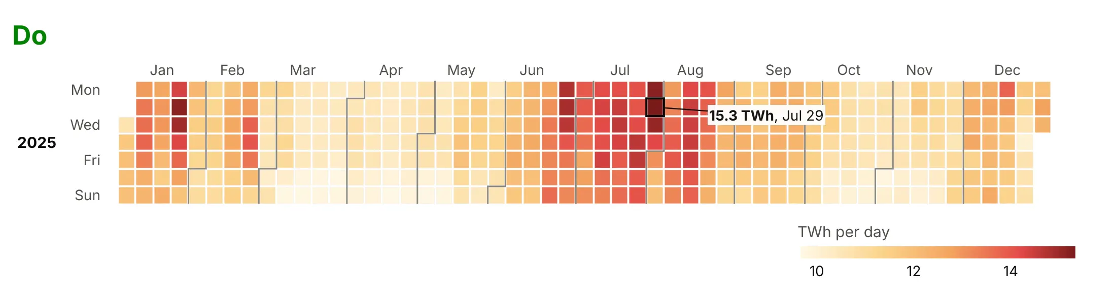
The quick way to a calendar heatmap is to pivot on isocalendar().week and pass the result to go.Heatmap. It gives a chart that is hard to read and silently wrong. Here is one year of US electricity demand both ways.

Don't pivot on ISO week numbers. ISO weeks put December 29-31, 2025 in week 1 (of 2026), so January's first column silently holds late-December days. The numbered axes don't say which row is Monday (here it's the bottom one) or where a month starts, and without gaps the weeks blur together:

Do count weeks from January 1, label the weekdays and months, draw month boundaries, leave small gaps between cells and label the day you talk about. The colors are the same as above:

Pick the color scale for the question

The biggest styling choice is the color scale. Here are four options on the same year of demand.

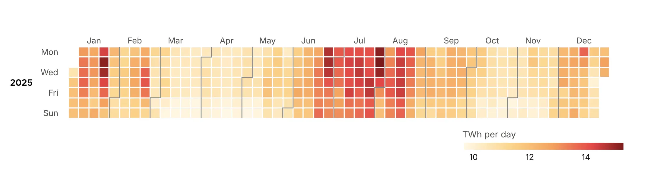
Sequential. The value itself, light to dark, which shows the seasons and the weekly rhythm and is a good default for amounts.

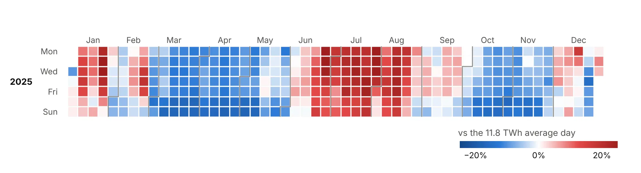
Diverging. Above or below a baseline, here the 2025 average day of 11.8 TWh, centered with cmid, so spring and fall turn blue and summer turns red.

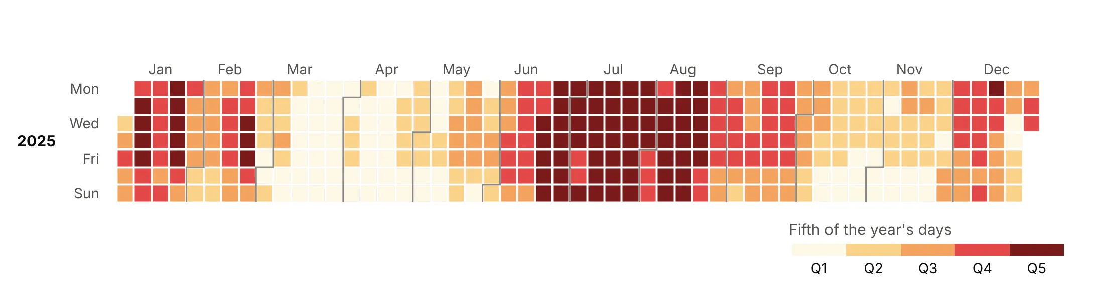
Binned. Five classes with the same number of days each, like GitHub's contribution levels, which makes each class easy to count.

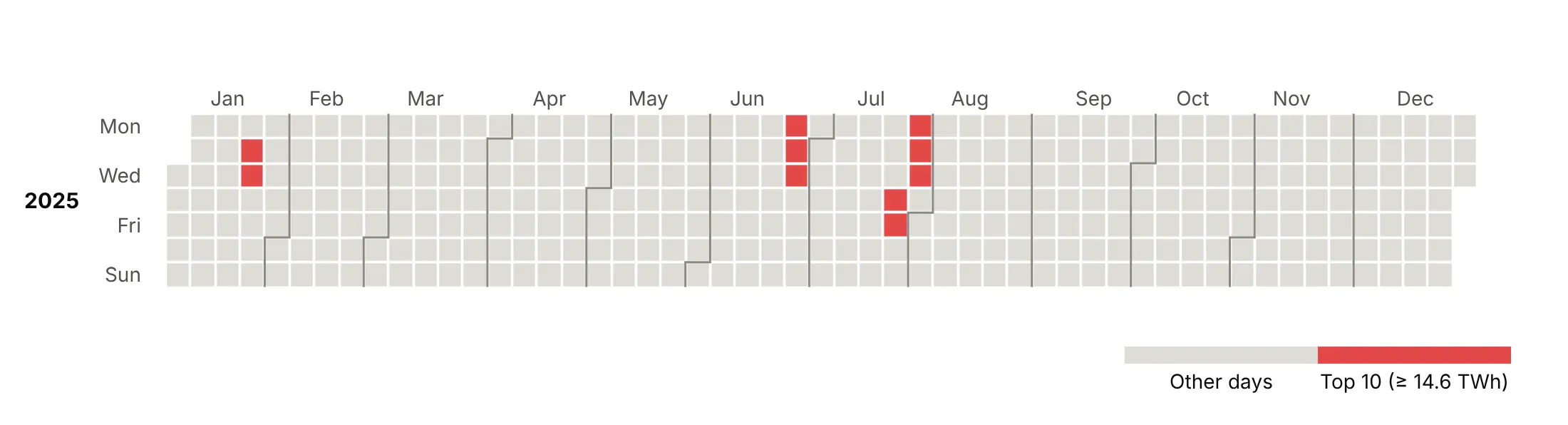
Highlight. Only the ten highest days in color, all at least 14.6 TWh, which shows that they came in three runs: January 21-22, June 23-25 and late July.

Checklist

Do

• Count weeks from January 1, not with ISO week numbers, and give each year its own row of subplots.
• Leave missing days gray and say so in the subtitle.
• Share one color axis across years (coloraxis) so a color means the same thing in every row.
• Center diverging scales on a meaningful value with cmid (zero, a normal, the average).
• Cap outliers with zmin and zmax and label the extreme day with its real value.
• Label the days you talk about with an outline and an arrow.

Don't

• Fill missing days with zero.
• Use a rainbow scale such as Jet for a quantity, because its bright bands look like boundaries in the data.
• Drop the weekday labels, because the rows are the point.
• Draw weekend rows for weekday-only data such as market prices; five rows are clearer.
• Rely on hover in a static image. Put the key numbers in the title or on labels.

Options to customize

These are the options that matter most for building a calendar heatmap from go.Heatmap, subplots and shapes. The full list is in the Plotly heatmap reference.

1. go.Heatmap(x, y, z) with 1-D arrays: one cell per (week, weekday) pair, which avoids pivoting and ISO week bugs.
2. xgap, ygap: the gap between cells in pixels; 1-3 px gives the calendar look.
3. coloraxis (trace) and layout.coloraxis: one shared scale for all year subplots.
4. colorscale, cmin, cmax, cmid: the scale, its caps and its center; cmid for diverging data.
5. Stepped colorscale: repeated stops give hard color classes for bins and thresholds.
6. hoverongaps=False: no hover on missing days.
7. customdata, hovertemplate: the date and a formatted value in the hover, since x and y are week numbers.
8. text with %{text}: the raw value in the hover when the color is a log or binned version of it.
9. make_subplots(rows=n_years): one row per year.
10. yaxis.autorange="reversed": Monday (or Sunday) on top.
11. yaxis.scaleanchor, scaleratio=1: square cells.
12. xaxis.tickvals, ticktext, side="top": month labels above the grid.
13. layout.shapes with type="path": step lines between months.
14. layout.shapes with type="rect", plus annotations: outline and label a day.
15. colorbar.orientation="h": a horizontal colorbar under a wide calendar.

More calendar heatmap examples

Ten more calendar heatmaps built from real public data, each with its source, the technique that makes it work and a prompt to rebuild it. All of them use the same helper as the Python example above.

1. The inverted yield curve

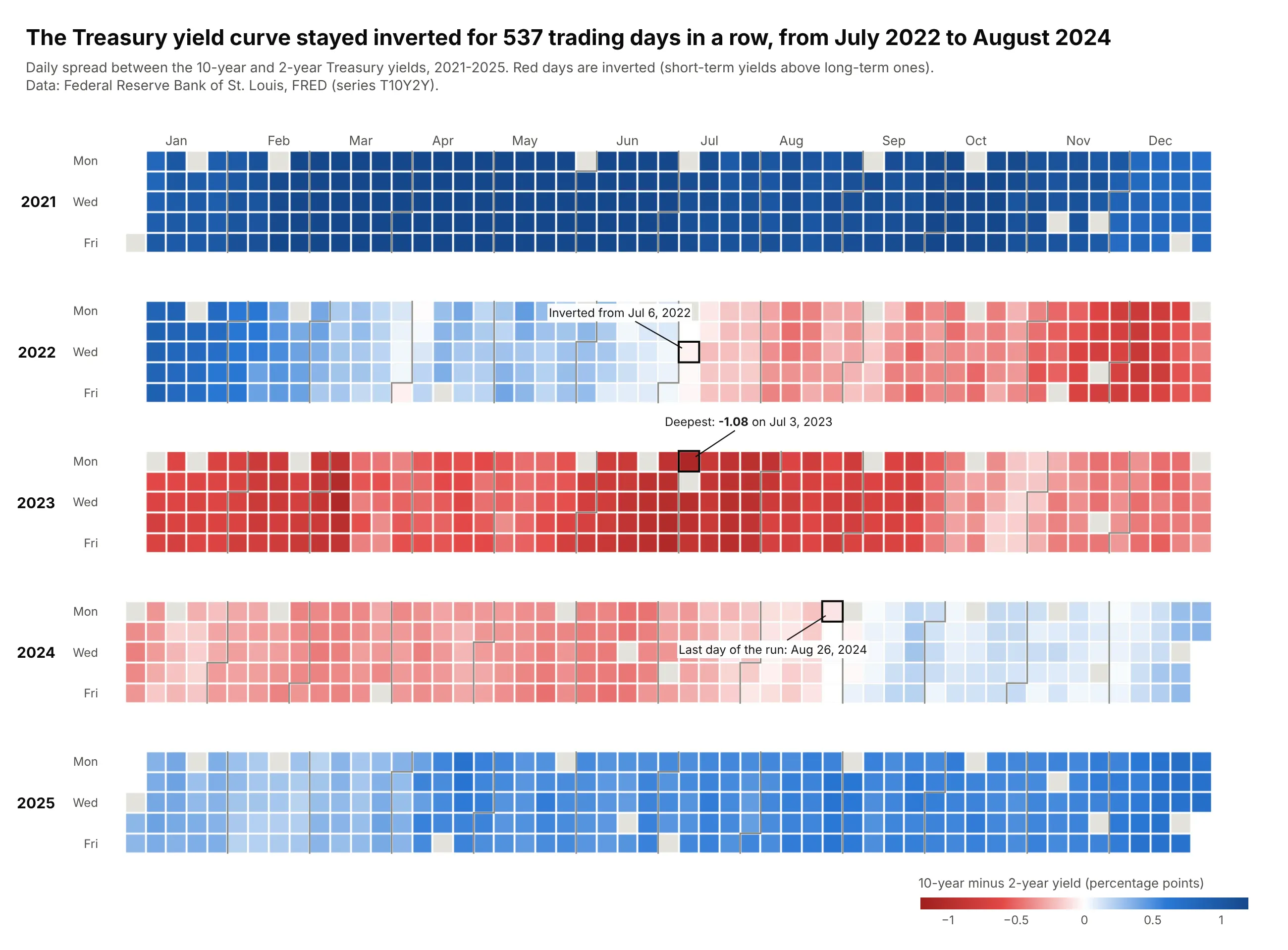
The 10-year minus 2-year Treasury spread was negative for 537 trading days in a row, from July 6, 2022 to August 26, 2024, and reached -1.08 points on July 3, 2023. On the calendar, the inversion is a red band that starts and ends on visible days. Data: Federal Reserve Bank of St. Louis, FRED (T10Y2Y), 2021-2025.

Tip: when the sign is the story, a diverging scale centered on zero turns a long run into one block of color.

2. Henry Hub natural gas

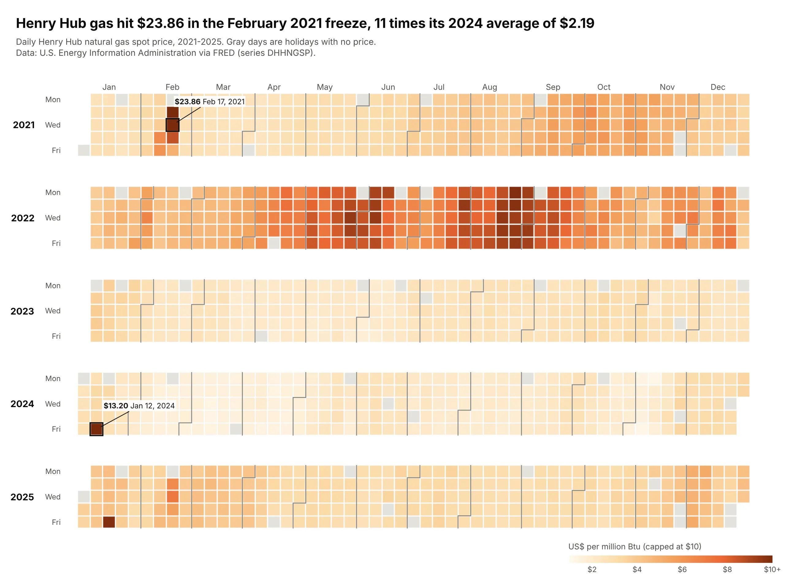
Henry Hub gas hit $23.86 in the February 2021 freeze, 11 times its 2024 average of $2.19. The calendar shows 2022's long expensive summer and how short the cold-snap spikes were, like $13.20 on January 12, 2024. Data: U.S. EIA via FRED (DHHNGSP), 2021-2025.

Tip: cap the scale at $10 and write the real price next to the capped days.

3. California solar

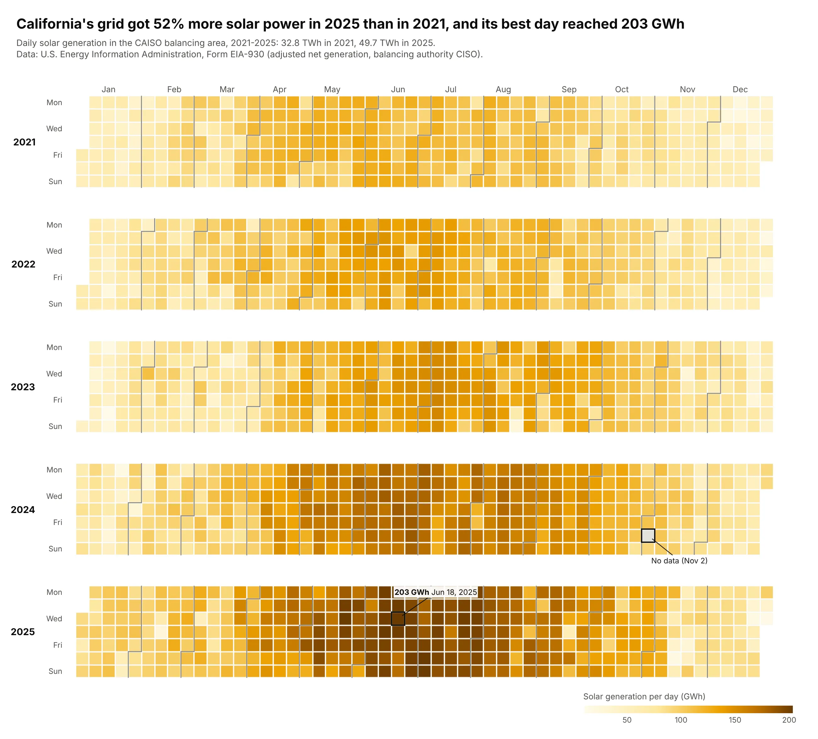
California's grid got 52% more solar power in 2025 (49.7 TWh) than in 2021 (32.8 TWh), and its best day reached 203 GWh. Each summer band is darker than the last, and winter storms show as single pale cells. Data: U.S. EIA, Form EIA-930 (CISO solar), 2021-2025.

Tip: treat impossible zeros as missing; the one 0 GWh day is a reporting gap, drawn gray and labeled.

4. Phoenix heat

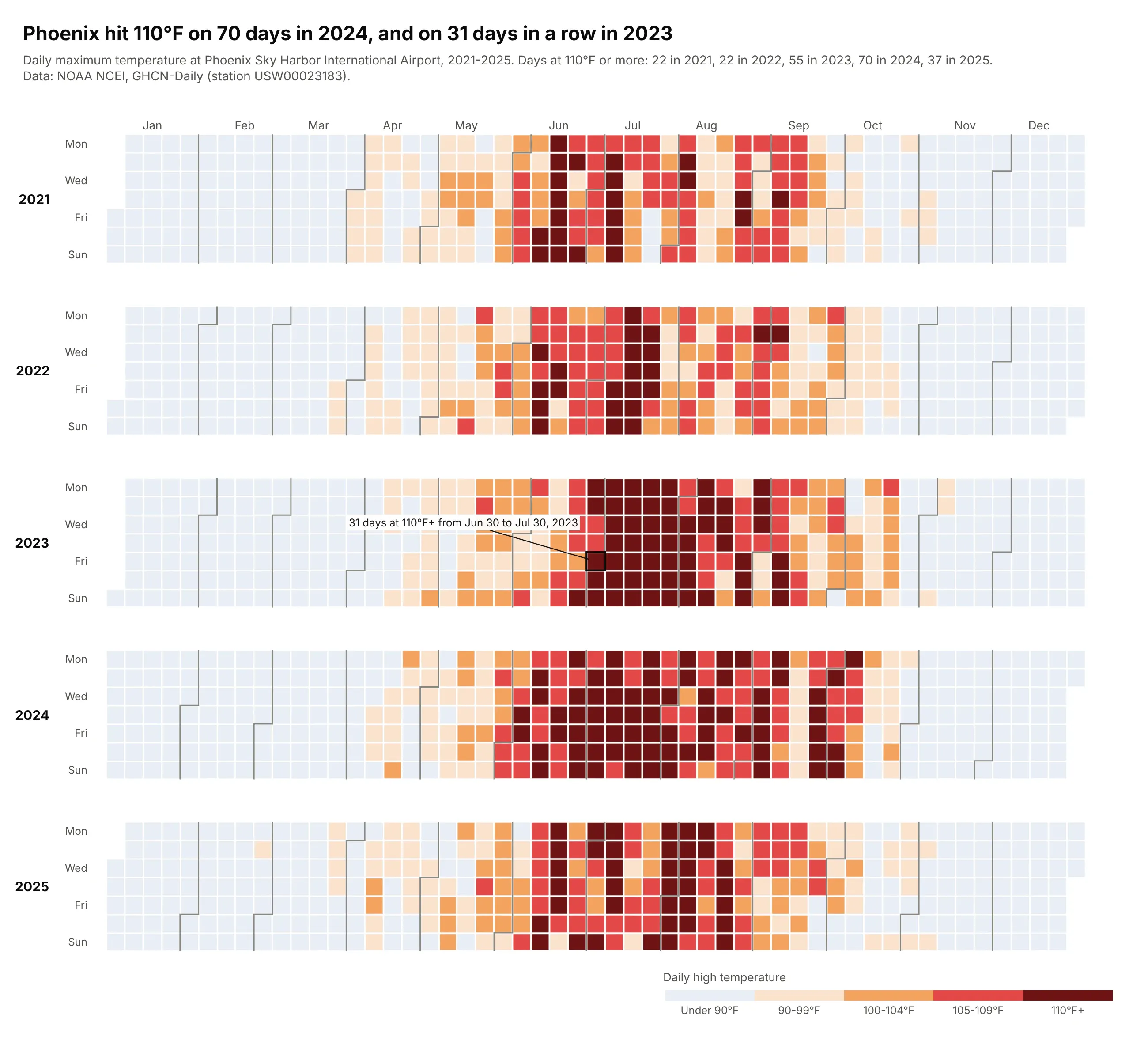
Phoenix hit 110°F on 70 days in 2024, up from 22 in 2021, and on 31 days in a row from June 30 to July 30, 2023. Binned colors make each run easy to count. Data: NOAA NCEI, GHCN-Daily, Phoenix Sky Harbor (USW00023183), 2021-2025.

Tip: five temperature classes on a stepped colorscale, so 110°F+ is one color instead of a shade.

5. Central Park temperature vs normal

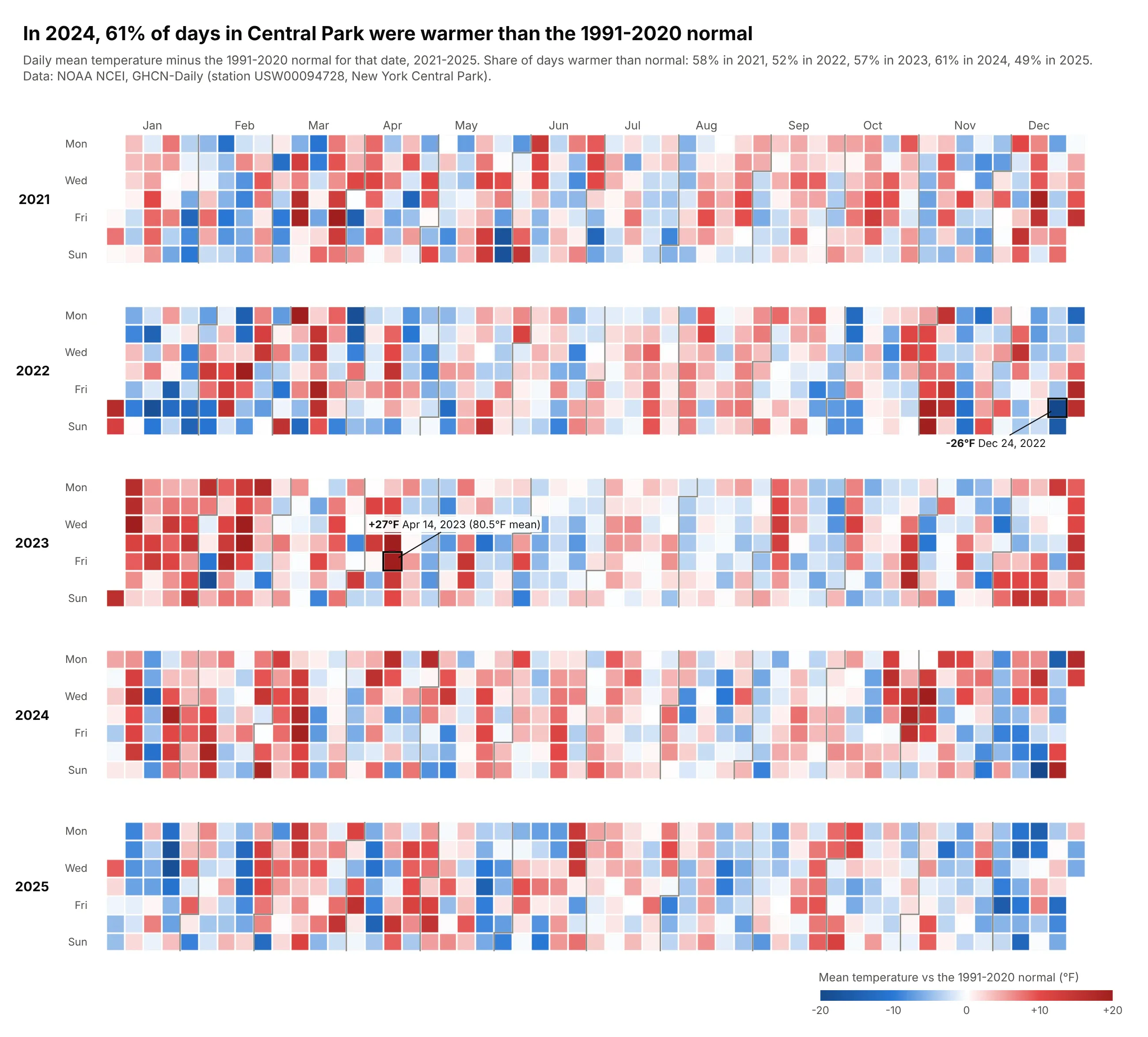
In 2024, 61% of days in Central Park were warmer than the 1991-2020 normal for their date. Warm and cold spells show as runs of red and blue, from +27°F on April 14, 2023 to -26°F on December 24, 2022. Data: NOAA NCEI, GHCN-Daily, New York Central Park (USW00094728), 1991-2025.

Tip: compute the normal per calendar date and smooth it with a 31-day window that wraps around New Year.

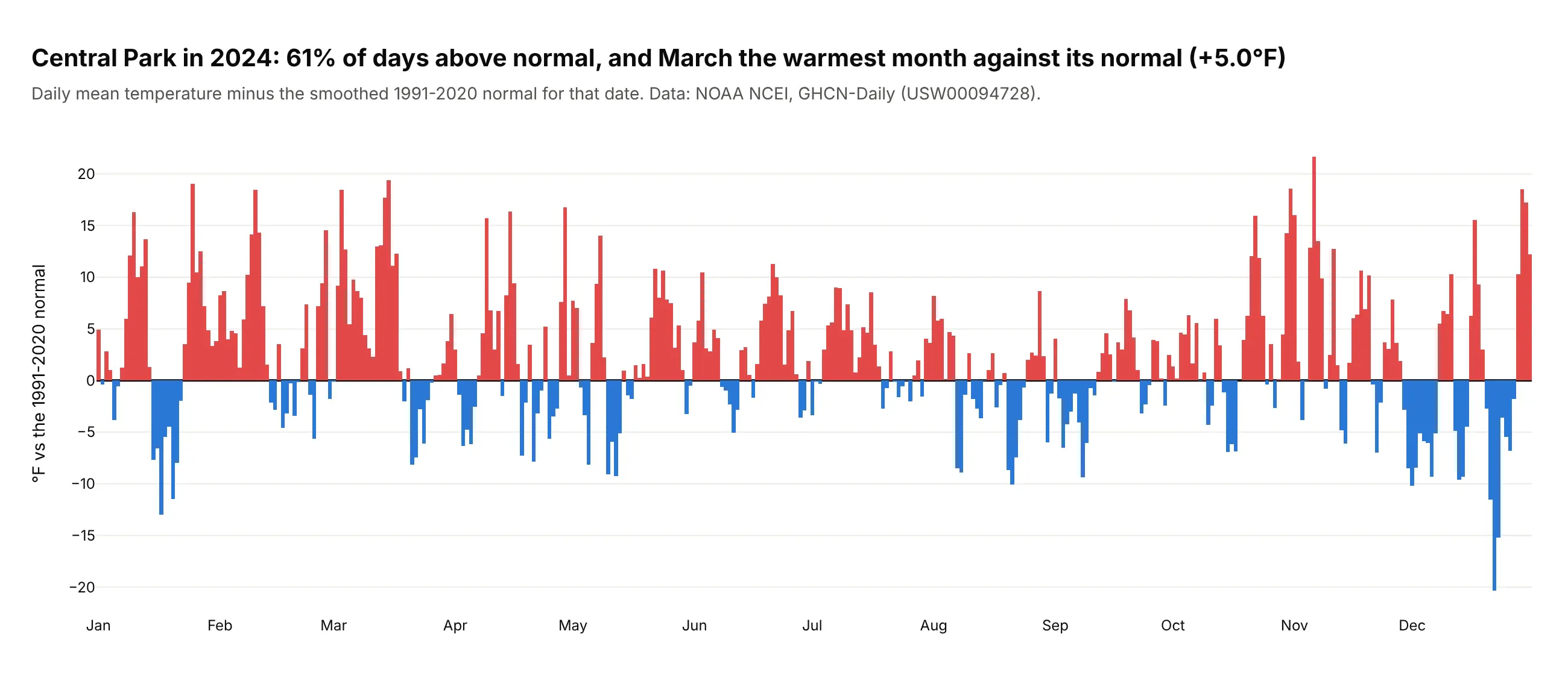
Another way to see it: bars of the 2024 anomalies show size better than color does. March was the warmest month against its normal, at +5.0°F on average.

6. Houston rain and Hurricane Harvey

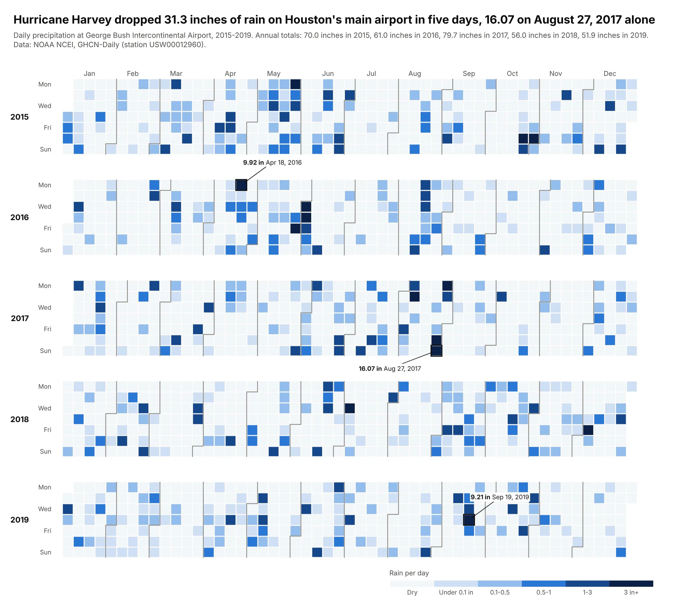
Hurricane Harvey dropped 31.3 inches of rain on Houston's main airport from August 25 to 29, 2017, 16.07 on August 27 alone. Rain is spiky, so most cells are pale dry days. Data: NOAA NCEI, GHCN-Daily, Houston Intercontinental (USW00012960), 2015-2019.

Tip: bins on a log-like ladder (0.1, 0.5, 1, 3 inches) instead of a linear scale, with dry days pale but visible.

7. COVID-19 case reports

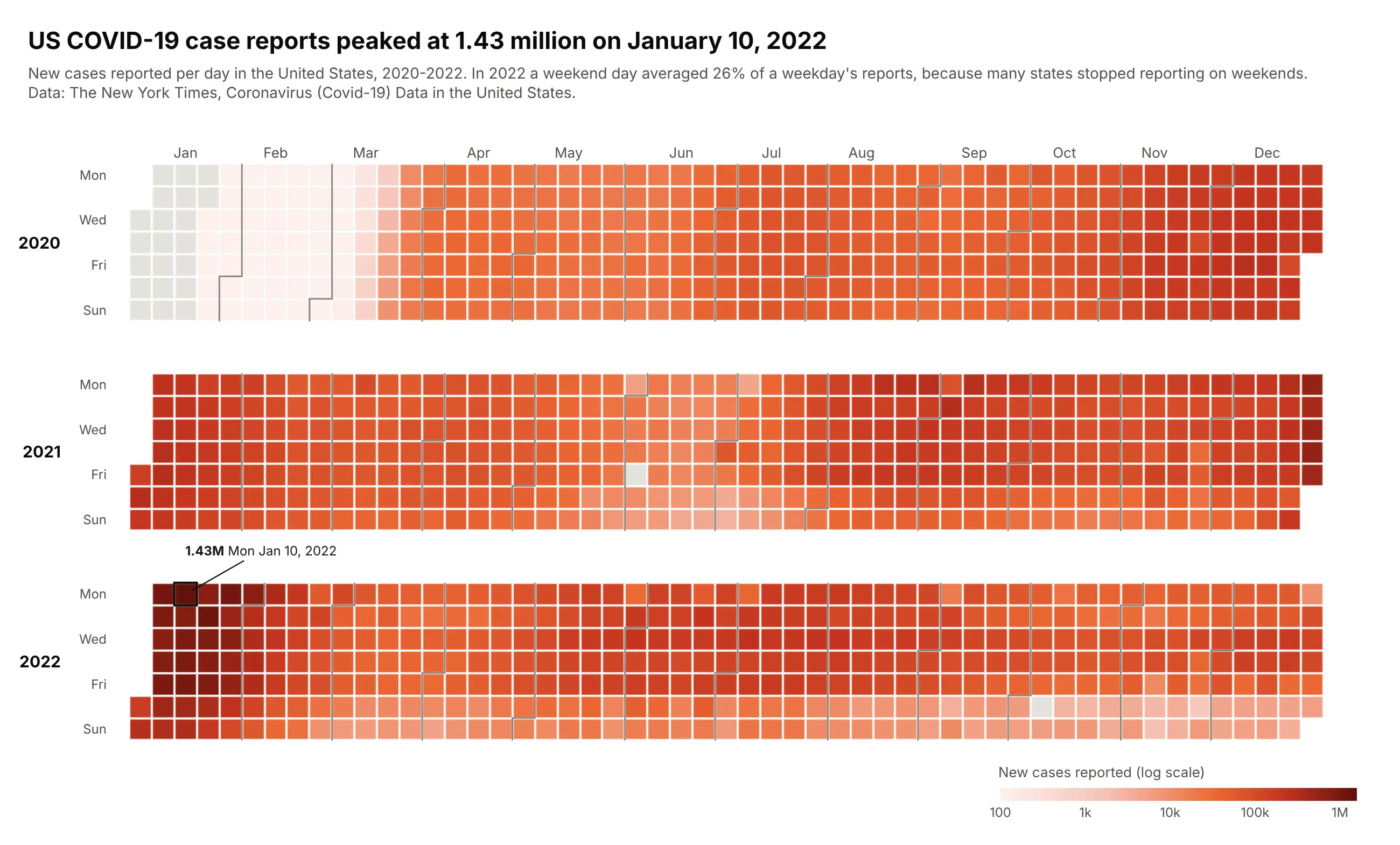
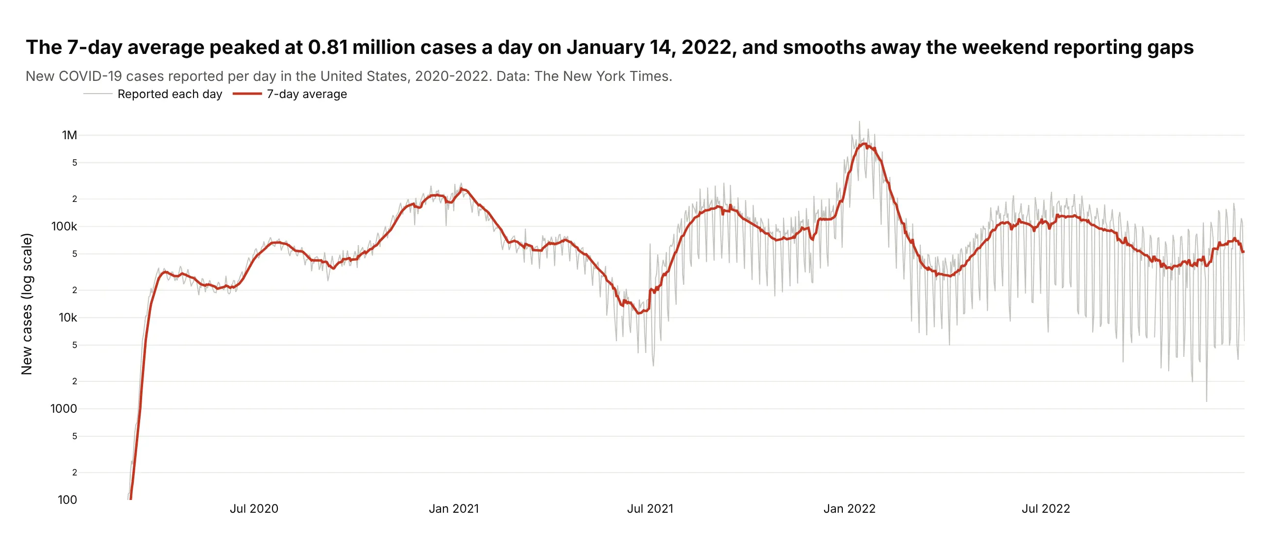
US COVID-19 case reports peaked at 1.43 million on Monday, January 10, 2022. In 2022 a weekend day averaged 26% of a weekday's reports, because many states stopped reporting on weekends, so the bottom rows go pale. Data: The New York Times, us.csv, 2020-2022.

Tip: a log color scale (log10 of the value, ticks labeled in real numbers, the raw count in the hover) for data spanning four orders of magnitude.

Another way to see it: a line chart with a 7-day average shows the waves more precisely and smooths the weekend gaps; the average peaked at 0.81 million a day on January 14, 2022.

8. FDA adverse event reports

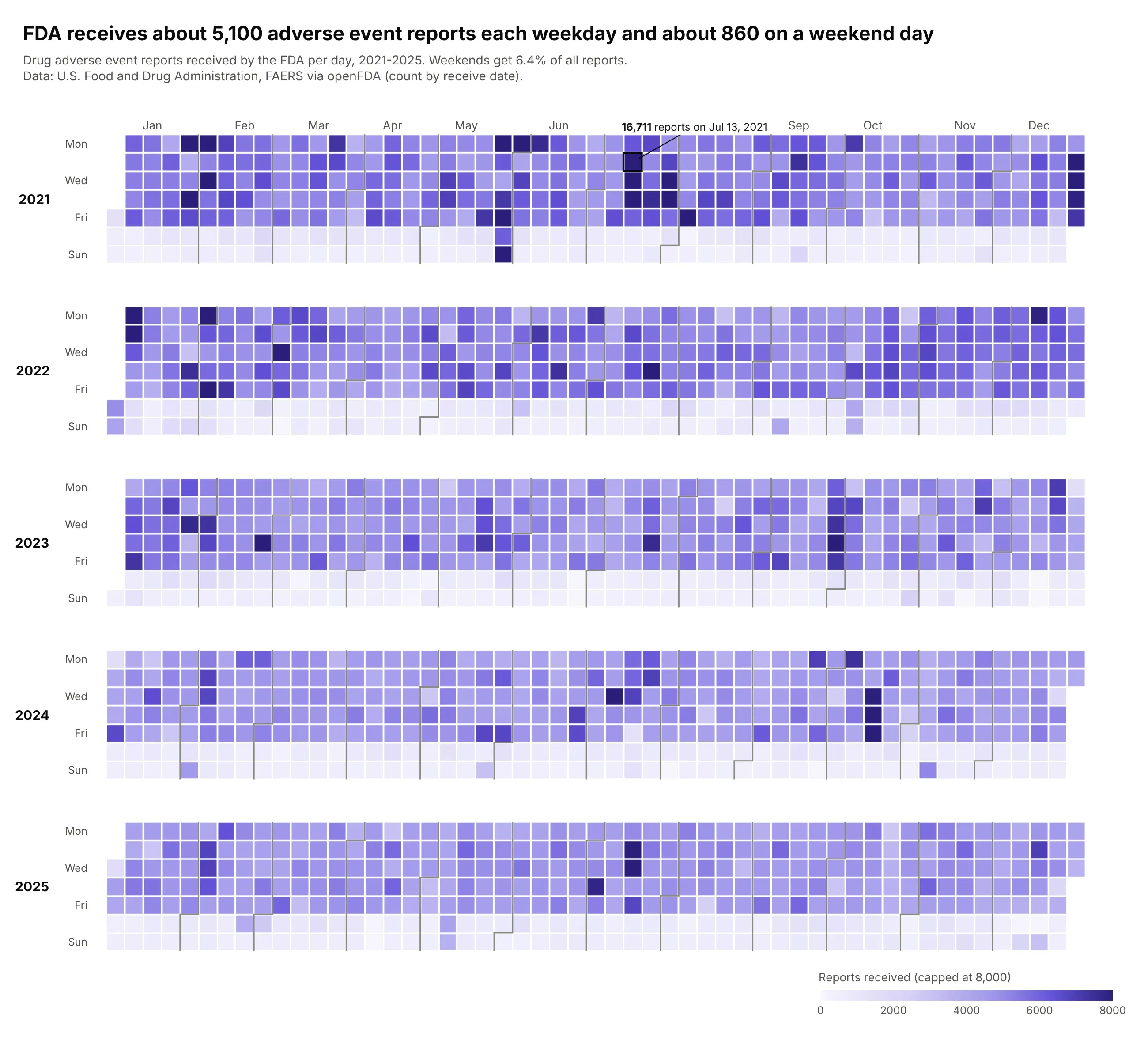
The FDA receives about 5,100 drug adverse event reports each weekday and about 860 on a weekend day, so weekends get 6.4% of all reports. The calendar shows when reports are filed, not when side effects happen. Data: FDA Adverse Event Reporting System via openFDA, 2021-2025.

Tip: cap the scale (here at 8,000) so a 16,711-report day doesn't flatten five years.

9. New York air quality and wildfire smoke

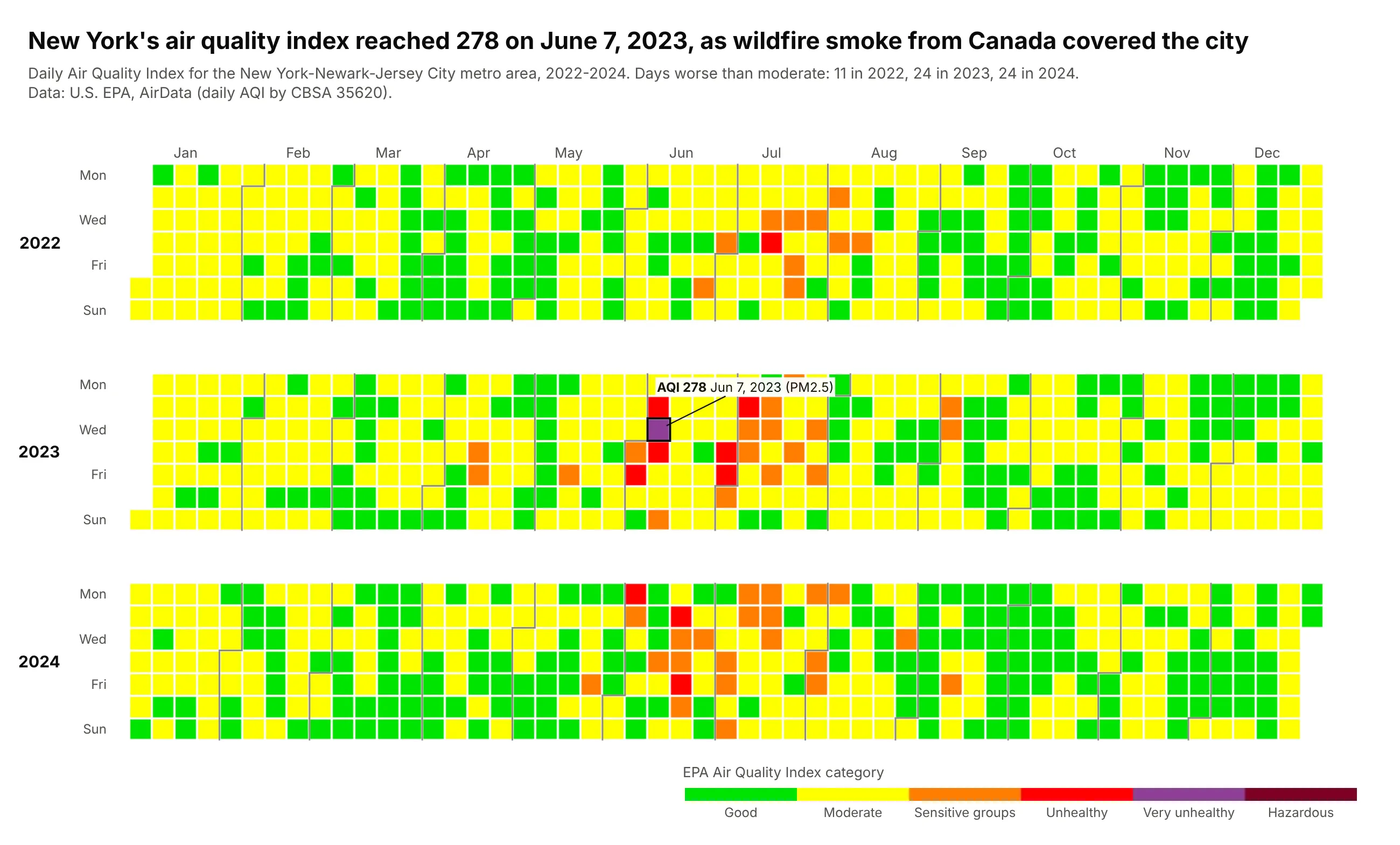
New York's air quality index reached 278 on June 7, 2023, when wildfire smoke from Canada covered the city, its only "very unhealthy" day in three years. The calendar shows that episode as a cluster in an otherwise green and yellow year. Data: U.S. EPA AirData, daily AQI by CBSA (35620), 2022-2024.

Tip: use EPA's own category colors on a stepped colorscale, because readers already know them.

10. Oklahoma earthquakes

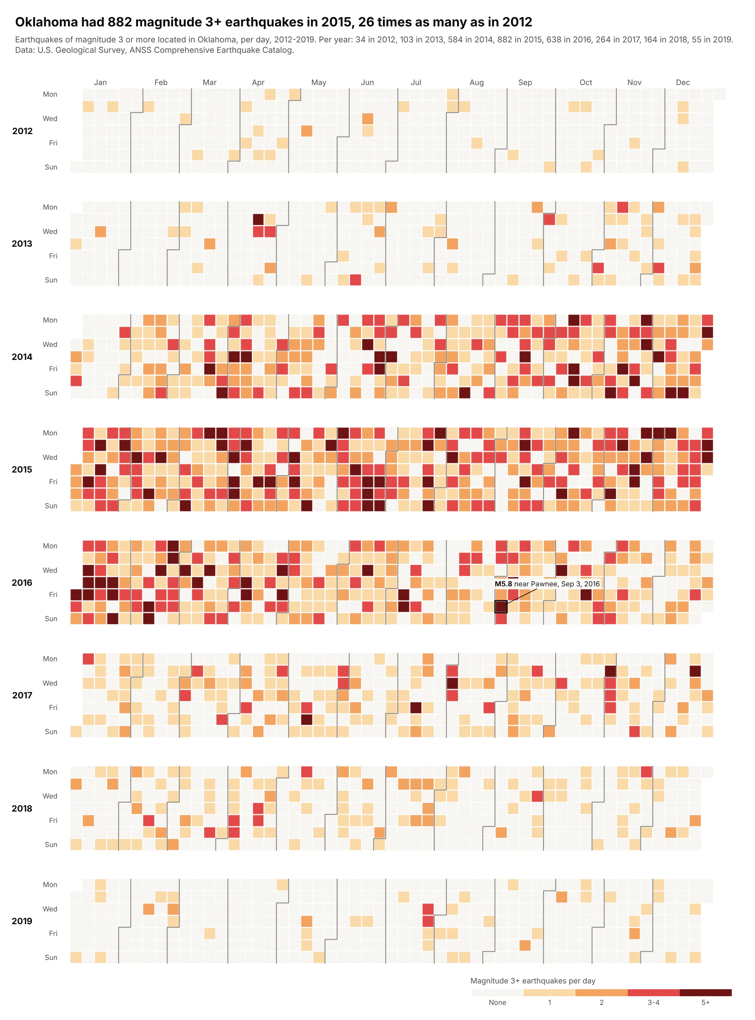
Oklahoma had 882 magnitude 3+ earthquakes in 2015, 26 times as many as in 2012, and 55 in 2019. Researchers linked the surge to wastewater injection from oil and gas production (Keranen et al., Science 2014). The largest, M5.8, struck near Pawnee on September 3, 2016. Data: USGS ANSS Comprehensive Earthquake Catalog, 2012-2019.

Tip: small counts in five classes (0, 1, 2, 3-4, 5+) and month labels only on the top row, which keeps eight years readable.