
Chris Parmer
November 18, 2026
Chromatograms - A Complete Guide
TL;DR
- A chromatogram is a line chart of what a detector sees as a mixture leaves a chromatography column: retention time (the minutes since injection) runs along the x axis, the detector's response runs up the y axis, and each compound draws one peak, so a peak's position says which compound it is and its area says how much of it there is.
- Chromatograms are named for the technique that makes them, such as high-performance liquid chromatography (HPLC) chromatograms and gas chromatography (GC) chromatograms, and they are similar to line charts, and to spectrograms and heatmaps when a second axis such as wavelength is added.
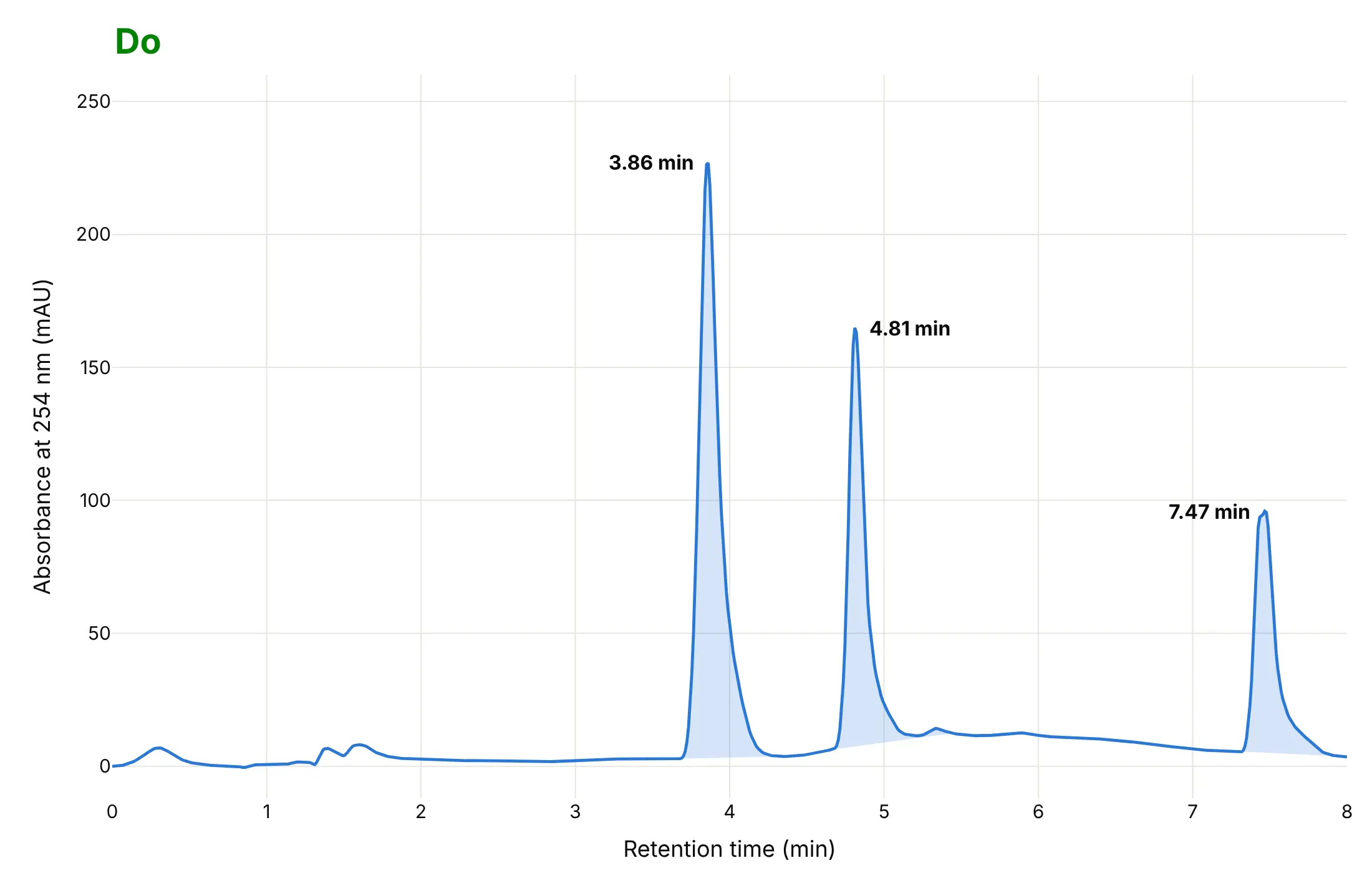
- Read them in this order: the baseline (the flat stretch with no compound leaving), then each peak's retention time, then its area, then whether neighboring peaks are separated. In an HPLC run of a reaction mixture the starting material's peak at 3.86 minutes has an area of 2,194 milli-absorbance-unit seconds (mAU·s) and the product's peak at 4.81 minutes has 1,266.
- Labs use them for purity and impurity profiling and for release testing of each batch: under the International Council for Harmonisation (ICH) Q3A guideline, an impurity in a new drug substance with a maximum daily dose of 2 g or less is reported above 0.05% of the peak area and has to be identified above 0.10% (or 1.0 mg a day, whichever is lower).
- You can make a chromatogram with Plotly in Python or JavaScript from a go.Scatter line, shade each peak's area with a filled polygon and label the peaks with annotations.
What is a chromatogram?
This is a chromatogram:
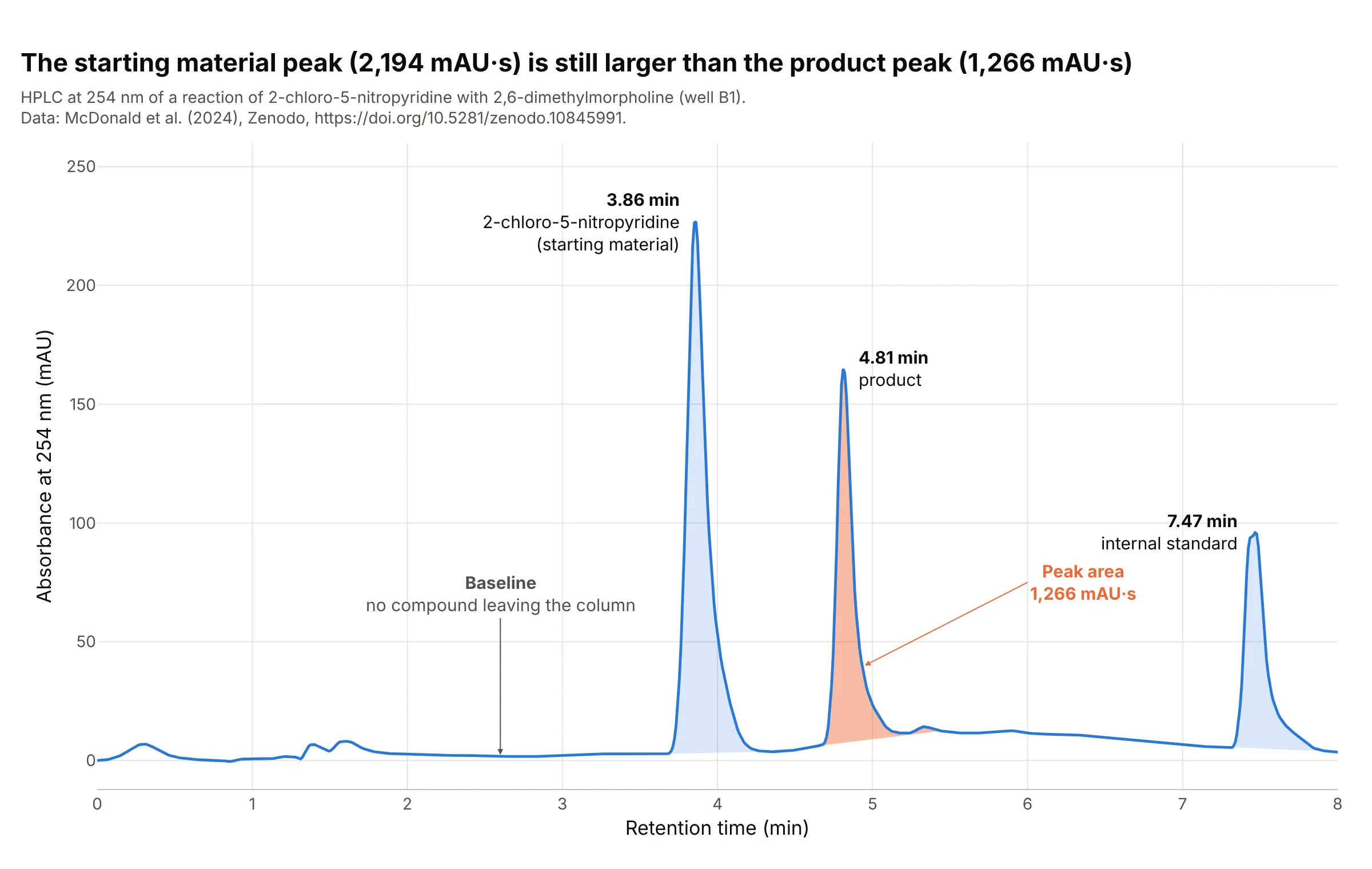
Data: McDonald et al. (2024), Zenodo, well B1 of reaction set 1: a Shimadzu Nexera HPLC with a photodiode-array detector (a detector that records the whole ultraviolet spectrum many times a second) and a mass spectrometer, run on a reaction of 2-chloro-5-nitropyridine with 2,6-dimethylmorpholine, the kind of reaction used to build drug-like molecules.
How do you read a chromatogram? In the example above, notice these things:
- The x axis is the retention time, the minutes between injecting the sample and the moment a compound reaches the detector, and every compound in the mixture has its own. The three peaks at 3.86, 4.81 and 7.47 minutes are three compounds: the starting material, the product and an internal standard, a compound added at the same level to every sample as a yardstick. We assigned the first two from the plate layout of the study, which the last answer of the FAQ explains.
- The y axis is the absorbance at 254 nanometers (nm), in milli-absorbance units (mAU), which is how much ultraviolet light the stream leaving the column absorbs. The three peaks are 227, 165 and 96 mAU tall. The data come as integers, and we divide them by 1,000 on the assumption that they are micro-absorbance units; the paper reports absorbance in absorbance units (AU).
- The baseline is the stretch where only solvent leaves the column. It is not zero: the median between 1.8 and 2.4 minutes is 2.4 mAU, and each peak is measured from a straight line under it, as the shading shows.
- The shaded area of a peak grows with the amount of that compound that passed the detector. The product's is 1,266 mAU·s (the area under the curve in mAU times seconds) and the starting material's is 2,194, so the starting material peak is 1.7 times bigger. The sizes are not amounts, though, because compounds absorb light differently: the product absorbs 1,522 mAU at 378 nm and only 165 mAU at 254 nm, about nine times less, so this view undercounts it.
- The peaks rise fast and fall slowly. The USP-style tailing factor (our calculation: the peak's width at 5% of its height over twice its front half-width) of the product's peak is 1.9, where 1 is a symmetrical peak.
It's often used for charts like these:
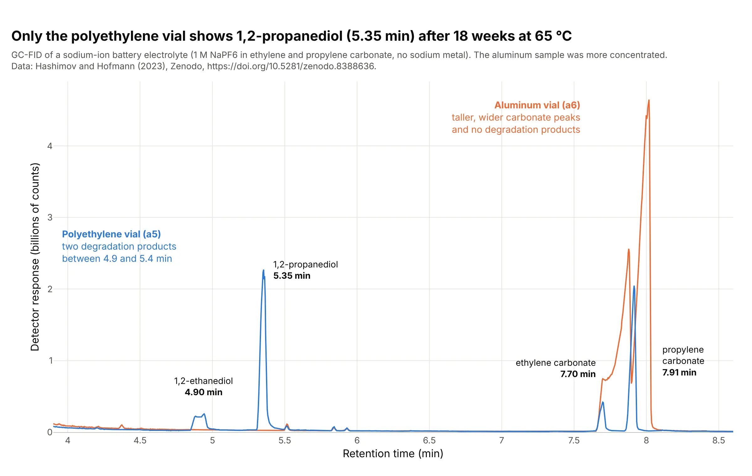
Overlaying a sample on a reference (the quality-control use). Drawing two runs on one time axis shows what appears in one and not the other, and it works because a compound leaves at the same retention time in every run. After 18 weeks at 65 °C, a sodium-ion battery electrolyte stored in a polyethylene vial has a 1,2-propanediol peak of 2.27 billion counts at 5.35 minutes and the sample stored in aluminum has none. Data: Hashimov and Hofmann (2023), Zenodo, a gas chromatograph with a flame ionization detector (FID, which burns the compounds and counts the ions), samples a5 and a6.
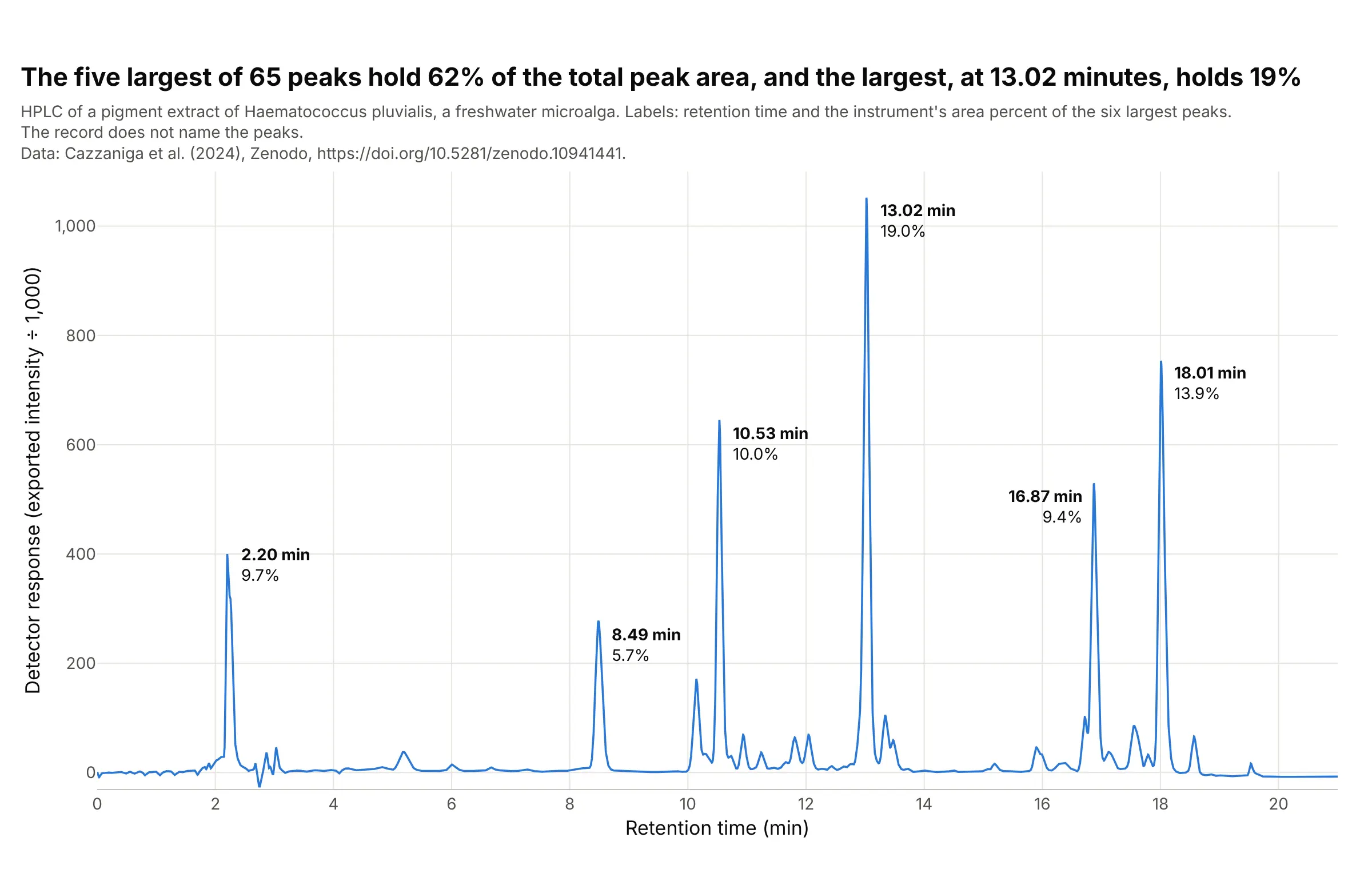
Plant pigments (the classic use). The first chromatography separated plant pigments, and the chromatogram of a microalga's pigment extract still looks like a crowded profile: of 65 peaks, the five largest hold 62% of the peak area and the largest, at 13.02 minutes, holds 19%. The instrument prints the report's retention time and area percent for each peak, and the record does not say which pigment is which, so the peaks are labeled by retention time alone, which is how unidentified peaks are reported. Data: Cazzaniga et al. (2024), Zenodo, a Jasco LC-4000 HPLC.
How to read a chromatogram from another field
The chart assumes a few ideas from analytical chemistry, and each of them sets one thing you see.
- Chromatography separates a mixture by letting it travel through a tube. The sample is injected into a flowing stream (the mobile phase, a liquid in HPLC and a gas in GC), which carries it through a column packed with a solid or coated with a liquid (the stationary phase). Each compound sticks to the stationary phase a little differently, so each leaves the column at its own time, and a detector at the end of the column turns what passes it into the line you see.
- Retention time is that time, from injection to the apex of the peak. It identifies a compound only by comparison: the same compound leaves at the same time under the same method, so labs run a reference standard (a pure sample of the compound) and match times, and confirm with a second detector such as a mass spectrometer. In the battery example the paper confirmed each peak against the pure compound.
- The detector sets the y axis. HPLC mostly measures how much ultraviolet light is absorbed (mAU). GC often uses a flame ionization detector, which gives a count roughly proportional to the carbon burned, and a mass spectrometer gives counts of ions, which can be drawn as the total ion chromatogram. The y axis is a response, not an amount, and different compounds give different responses, which is why the ICH guideline asks for a correction factor when the response of an impurity and the drug substance are not close.
- A gradient or a temperature program changes the conditions during the run so that late compounds do not take forever. The HPLC runs here raise the share of acetonitrile in water from 5% to 100% over the run (according to the paper), and the GC oven goes from 40 °C to 320 °C at 20 °C a minute. This is why a baseline can drift during a run.
- Peak area is the integral of the peak above the baseline. Software finds the start and end of each peak and draws a straight line under it, and that valley-to-valley line is a choice, so methods fix it. The area percent is one peak's share of the total of all peaks.
- An internal standard is a compound added in the same amount to every sample. Dividing a peak's area by the standard's corrects for how much was injected, as example 3 below shows.
- Resolution (Rs) says how well two neighboring peaks are separated: Rs = 2 (t2 - t1) / (w1 + w2), where t is the retention time and w the peak width at the base. Measuring widths at half height gives Rs = 1.18 (t2 - t1) / (w1 + w2), which is what example 2 below uses. An Rs of 1.5 or more is the usual target for baseline separation.
A short history
Mikhail Tsvet separated plant pigments such as chlorophyll, carotenes and xanthophylls in the first years of the twentieth century, and the pigments separated in colored bands, which is why the technique is named for color. He published the method in Berichte der Deutschen Botanischen Gesellschaft in 1906 (the year and journal as Crossref lists them; Wikipedia dates the work to 1901 to 1905). Martin and Synge described partition chromatography in 1941, which won them a share of the 1952 Nobel Prize in Chemistry, and James and Martin described gas-liquid chromatography in 1952, which led to the GC chromatograms in this guide. We could not find Tsvet's original columns in a form that could be redrawn, so the history here stays in words, and the pigment extract shown above is a modern HPLC separation of the same kind of sample.
Alternatives to a chromatogram
Here's the same HPLC run drawn six ways. Some are better for the question, some worse, some just different:
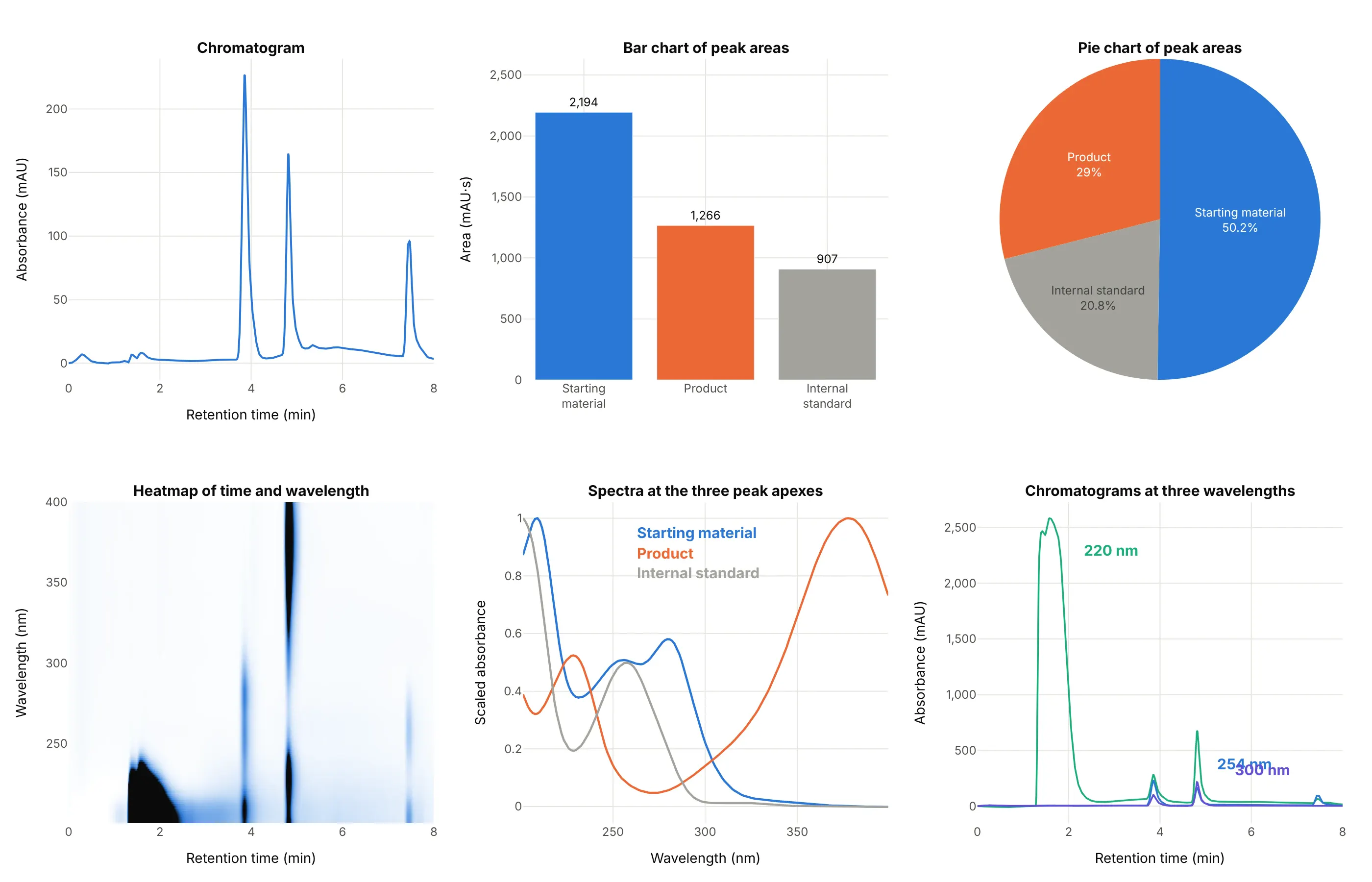
- Chromatogram at one wavelength (the standard view). It keeps the retention time that identifies a peak and the shape that shows tailing and overlap, which no summary below keeps.
- Bar chart of peak areas (works too, for comparing samples). After integration, bars make it easy to compare the same peak across many runs, but they drop the retention times and cannot show a peak that is half hidden by its neighbor.
- Pie chart of peak areas (worse). It turns area into a share of the total, which is the area percent a report prints, but shares of different compounds depend on how strongly each absorbs light, and here the internal standard takes 21% of the pie for a compound that is not part of the sample.
- Heatmap of time and wavelength (different). A photodiode-array detector records a whole spectrum at every moment, and the heatmap shows all of it at once: the product shows as a dark band at 4.8 minutes that reaches 378 nm, which is how you find the best wavelength. It is the same idea as a spectrogram, with wavelength where frequency would be.
- Spectra at the peak apexes (different). A spectrum identifies a compound by its shape instead of its time, and comparing the spectrum across one peak is how purity is checked (example 5 below).
- Chromatograms at several wavelengths (works too). At 220 nm the solvent front in the first two minutes reaches about 2,600 mAU and swamps the peaks, while at 300 nm the trace is quiet, so picking a wavelength is part of the method.
How to make a chromatogram
With AI
ChatGPT, Claude Code, GitHub Copilot, Cursor and other AI tools are excellent at writing Plotly code. Name Plotly in the prompt, and say how to find the peaks and what to label:
Make a plotly chromatogram from hplc_B1.csv (columns: time_min, absorbance_mau).- Draw one thin line, retention time in minutes on x and absorbance at 254 nm in mAU on y.- Find the peaks with scipy.signal.find_peaks (prominence 30) and label each with its retention time.- Shade the area of each peak down to a straight baseline between its start and end, and write thearea in mAU·s next to the biggest peak.- A title that states the takeaway, with the source in a muted subtitle.
With Plotly Studio
Plotly Studio is a product for creating data visualizations and Dash apps and for analyzing data with AI, available as a desktop app or embedded in Dash apps. Ask for a chromatogram viewer the same way:
Show my HPLC runs as chromatograms, retention time on x and absorbance on y, with a dropdown to pick a run, a second dropdown to overlay a reference standard, peaks labeled with retention time and area, and a slider for the baseline.
Make a chromatogram in Python or JavaScript
This is the code AI tools write under the hood. In Python, scipy.signal.find_peaks finds the apexes, a function integrates a peak above a straight baseline, and go.Scatter draws the line:
import numpy as npimport pandas as pdimport plotly.graph_objects as gofrom scipy.signal import find_peaksrun = pd.read_csv("hplc_B1.csv") # time_min, absorbance_maut, y = run.time_min.to_numpy(), run.absorbance_mau.to_numpy()peaks, _ = find_peaks(y, prominence=30) # apexes of the tall peaksdef area(t, y, start, end):"""Peak area in mAU*s above a straight baseline from the start to the end of the peak (valley to valley)."""m = (t >= start) & (t <= end)base = np.interp(t[m], [start, end], [y[m][0], y[m][-1]])return np.trapezoid(y[m] - base, t[m] * 60)fig = go.Figure(go.Scatter(x=t, y=y, mode="lines", line=dict(color="#2a78d6", width=2)))for p in peaks:fig.add_annotation(x=t[p], y=y[p], text=f"<b>{t[p]:.2f} min</b>", showarrow=False, yshift=14)fig.update_layout(xaxis_title="Retention time (min)", yaxis_title="Absorbance at 254 nm (mAU)", template="plotly_white")fig.show()print(round(area(t, y, 4.34, 5.45))) # the product peak, about 1,270 mAU·s
To shade a peak, add a trace with fill="toself" whose x and y go along the curve and back along the baseline, as the guide's examples do. For a full spectrum per time point, draw the matrix with go.Heatmap(x=times, y=wavelengths, z=absorbance.T).
In JavaScript, plotly.js draws the same chart. This example reads the same CSV and labels each tall peak:
<div id="chart"></div><script src="https://cdn.plot.ly/plotly-4.1.1.min.js"></script><script>fetch("hplc_B1.csv").then(r => r.text()).then(text => {const rows = text.trim().split("\n").slice(1).map(line => line.split(",").map(Number));const t = rows.map(r => r[0]), y = rows.map(r => r[1]);// apexes: the highest point within 15 samples (about 10 seconds) on each side, taller than 50 mAUconst apexes = [];for (let i = 15; i < y.length - 15; i++) {const window = y.slice(i - 15, i + 16);if (y[i] > 50 && y[i] === Math.max(...window)) apexes.push(i);}Plotly.newPlot("chart", [{x: t, y: y, mode: "lines", line: {color: "#2a78d6", width: 2}}], {width: 800, height: 480, showlegend: false,xaxis: {title: {text: "Retention time (min)"}},yaxis: {title: {text: "Absorbance at 254 nm (mAU)"}},annotations: apexes.map(i => ({x: t[i], y: y[i], text: `<b>${t[i].toFixed(2)} min</b>`, showarrow: false, yshift: 14}))});});</script>
Instrument software exports chromatograms in many layouts. A Shimadzu LabSolutions text export, as in the guide's first dataset, holds a header and then a table of time against wavelength, and a Jasco export is a semicolon-separated file with a comma as the decimal mark, so pd.read_csv(..., sep=";", decimal=",") reads it. Open formats such as netCDF (.cdf) and mzML hold chromatograms from mass spectrometers.
Share it
Every Plotly chart has a Share chart button (the cloud icon in its toolbar) that uploads it to Plotly Cloud and gives you a link. Only you can see it until you change its visibility.
For a live app, put the chart in a Dash app and publish it with the Plotly Cloud command-line interface (CLI). Coding agents can run these commands for you:
pip install "dash[cloud]"plotly user loginplotly app publish
If your data has to stay in your own cloud or data center, publish to Dash Enterprise instead.
Dos and don'ts
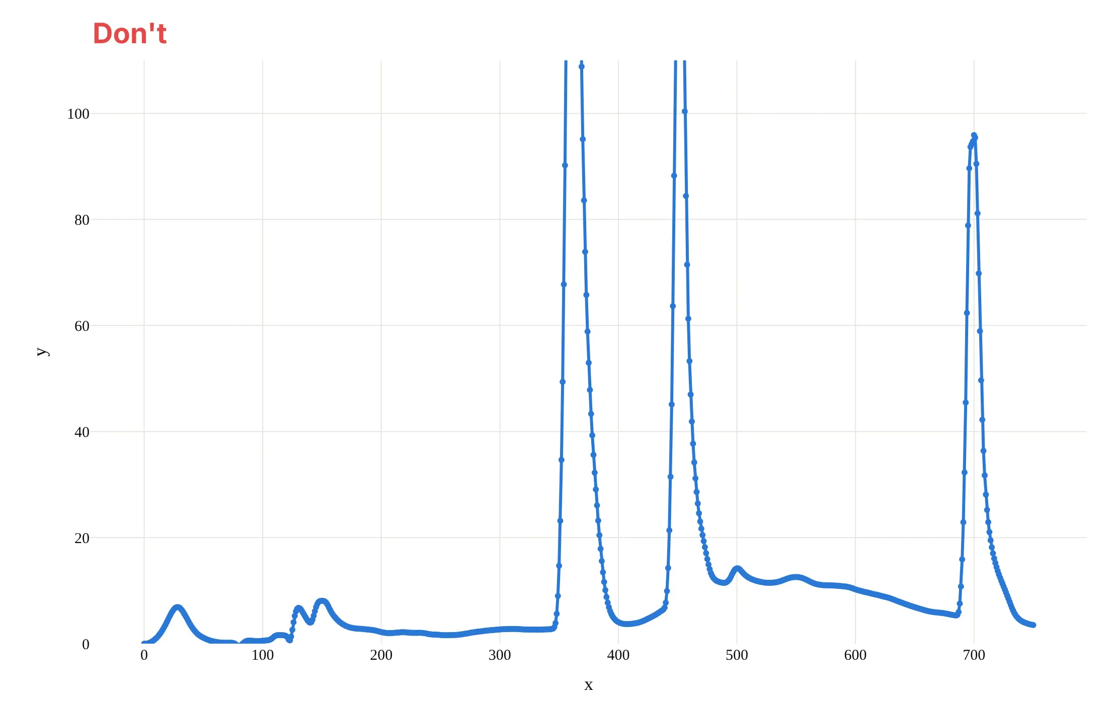
A chromatogram is read by position and by area, so most of the work is showing every peak whole, in minutes, with a baseline you can see. Here is the same run both ways, in the same color.
Don't plot against the sample number instead of minutes, clip the y axis so the tall peaks run off the top, leave the axis titles as x and y, draw thick lines with a marker on every point, or use a default serif font:
Do put retention time in minutes on the x axis, show the whole signal with a little room below the baseline, title the axes with the quantity and the unit, use a thin line, shade each peak's area down to its baseline and label the retention times:
Checklist
Do
- Put retention time on the x axis in minutes, and the detector response with its unit on the y axis.
- Show the baseline, and zoom into it separately if you need to (example 1 below).
- Label peaks by retention time, and by name only when a reference standard confirmed it.
- Say which detector, wavelength and method produced the trace, because the same sample looks different at 220 nm and at 378 nm.
- Compare runs on one axis only when the method is the same, and scale by an internal standard when the amounts differ (examples 3 and 6 below).
Don't
- Read the size of a peak as the amount of a compound without a standard or a response factor.
- Compare retention times between methods, or between columns, as if they were the same measurement.
- Call two peaks separated without looking at the valley between them or computing Rs (example 2 below).
- Smooth the trace until the tailing and the shoulders that tell you about the run disappear.
More chromatogram examples
Seven more chromatograms and chromatogram-derived charts built from real public data, each with its source, a tip and a prompt to rebuild it.
1. The baseline is not zero
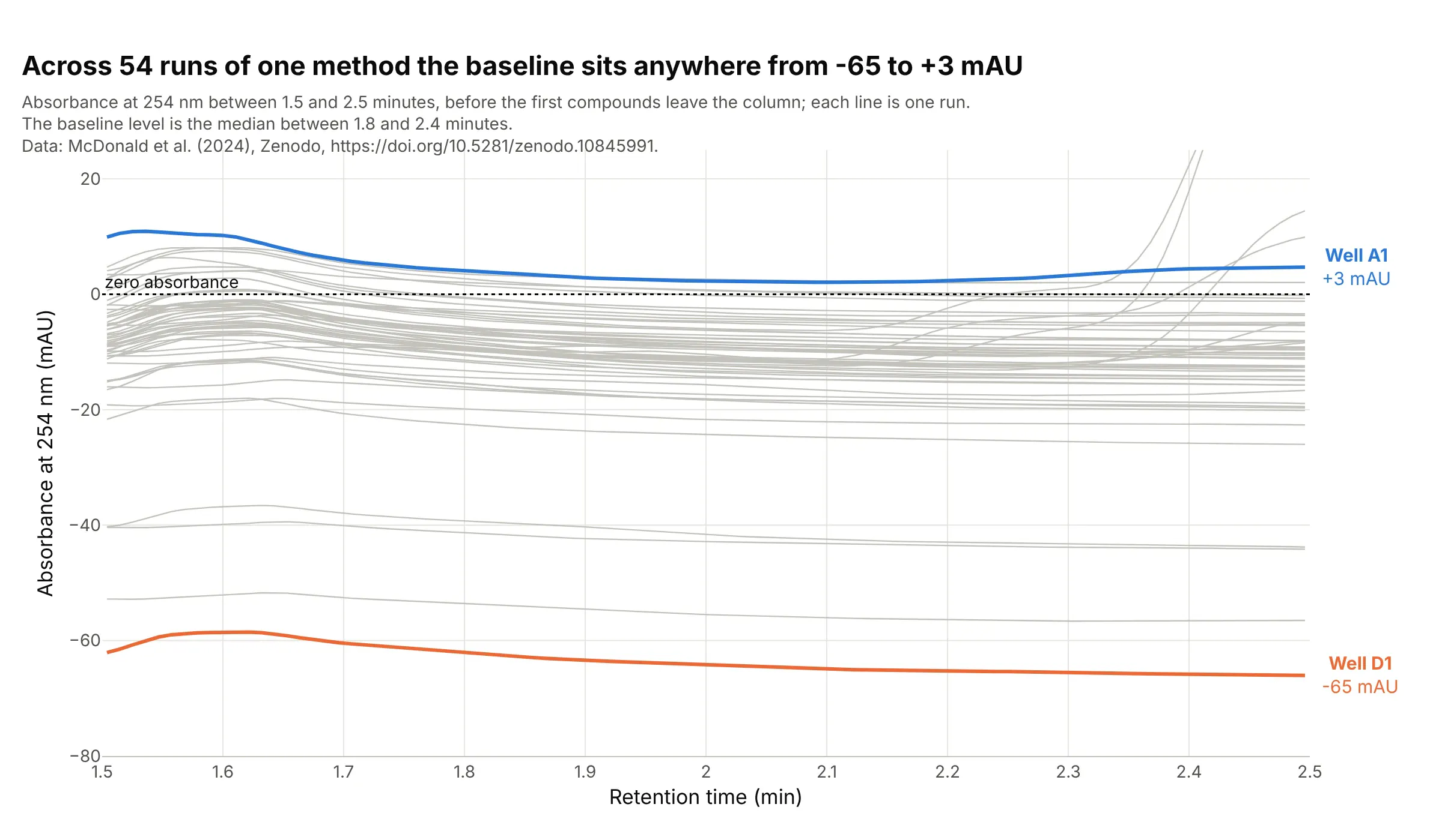
The baseline is the signal when only solvent is leaving the column, and across 54 runs of one method it sat anywhere from -65 mAU (well D1) to +3 mAU (well A1) between 1.8 and 2.4 minutes, with most of the runs near -10 mAU. Integration software measures each peak from the baseline under it, so a 100 mAU peak is 100 mAU above its own baseline, not above zero. Data: McDonald et al. (2024), all 54 reaction wells of reaction set 1.
Tip: zoom into the quiet stretch before the first peak and draw the zero line, so the offsets between runs are visible.
Get the data from the Zenodo record doi 10.5281/zenodo.10845991 (McDonald et al. 2024), file reaction_set_1.zip: theShimadzu LabSolutions exports PDA_Data_002.txt to PDA_Data_055.txt (a [PDA 3D] section with a header row ofwavelengths multiplied by 100 and one row per time point; the well is in the Data File Name header).Take the column closest to 254 nm of each file, divide the integers by 1,000 and make a plotly line chart of all 54 wells,x from 1.5 to 2.5 minutes, light gray lines, the highest and lowest baseline (median between 1.8 and 2.4 minutes)in color with their well labels, and a dotted line at zero.
2. Resolution: when two peaks are really two peaks
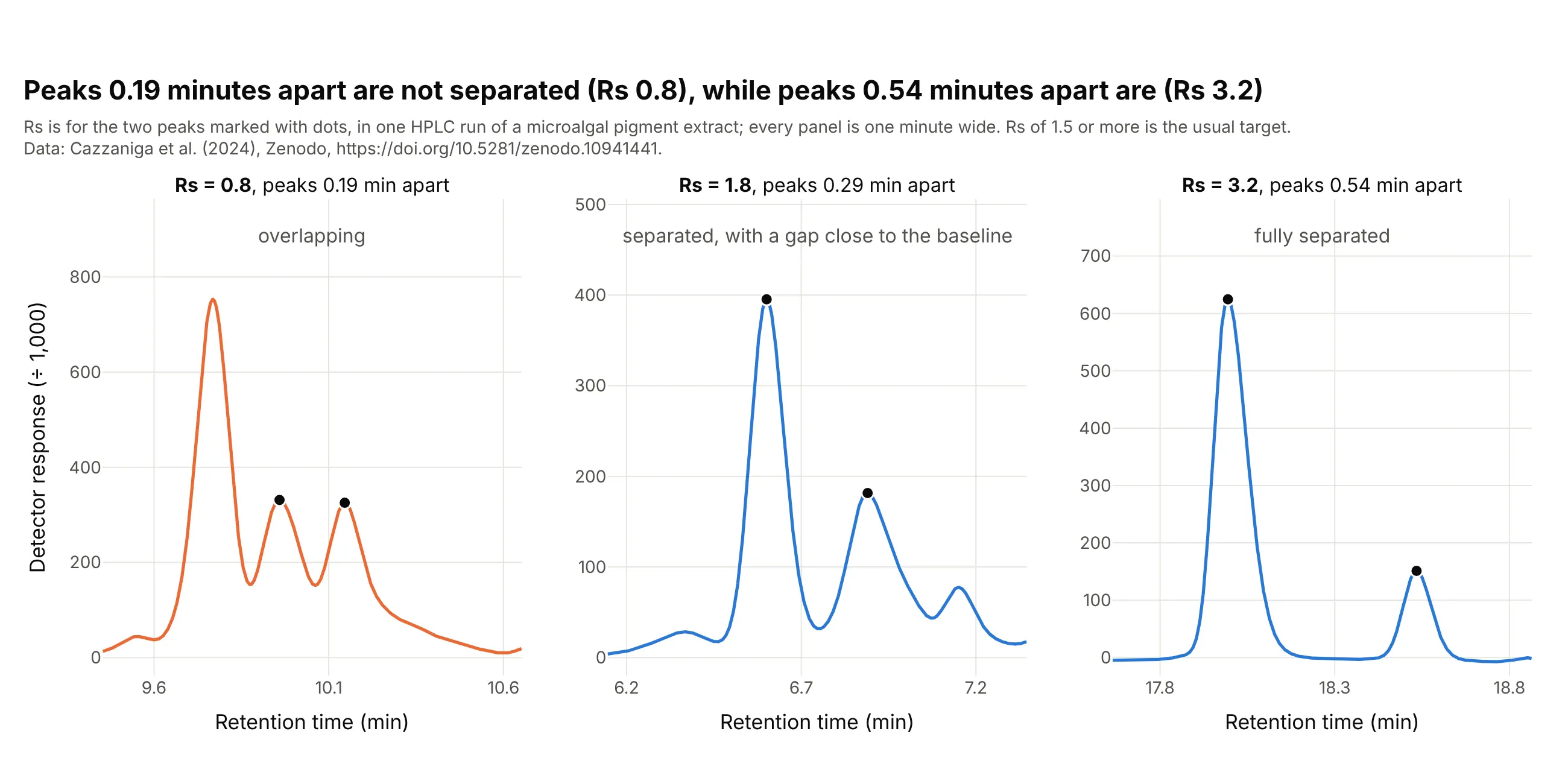
Resolution (Rs) turns "do these peaks overlap?" into a number. In one pigment run, two neighboring peaks 0.19 minutes apart have an Rs of 0.8, a pair 0.29 minutes apart has 1.8, and a pair 0.54 minutes apart has 3.2, so only the last two clear the usual 1.5 target. Data: Cazzaniga et al. (2024), Nannochloropsis gaditana S4 broken cells.
Tip: draw every pair on the same width of time, so the eye compares spacing and not zoom, and write the Rs on the panel.
Get the data from the Zenodo record doi 10.5281/zenodo.10941441 (Cazzaniga et al. 2024): "S4 Broken cell.csv" (semicolonseparated, comma decimal; columns min and Intensity) and the Jasco "Peaks Report.csv" (columns tR, Area, Height, Area%).Make a plotly figure with three panels of one minute each, centered on the neighbor pairs 9.959 and 10.146 minutes, 6.601 and6.890 minutes, and 17.994 and 18.534 minutes. Mark the two peaks with dots and write Rs = 1.18 (t2 - t1) / (w1 + w2) ineach title, with w the half-height width of each peak.
3. Dividing by an internal standard
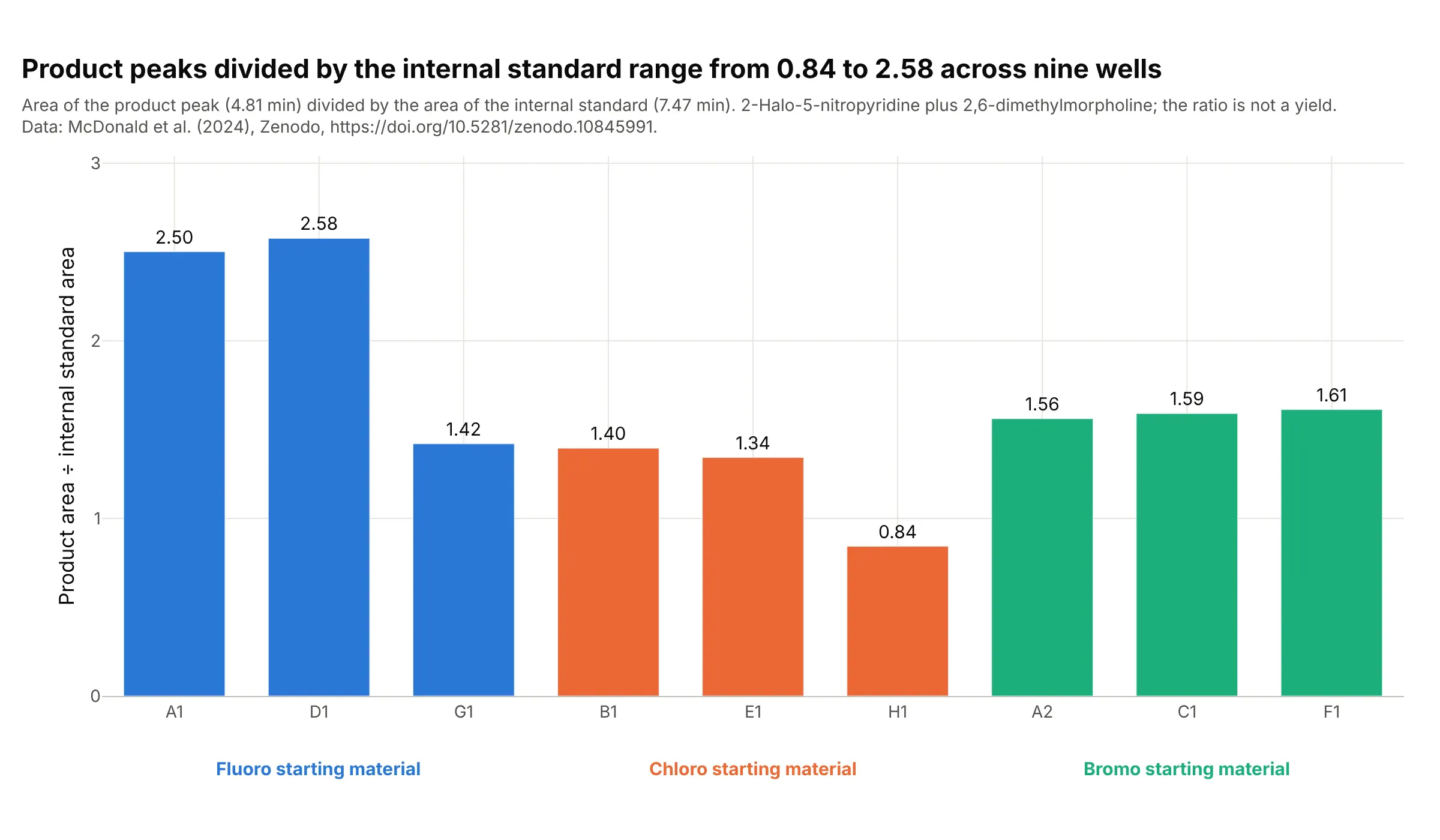
An area depends on how much sample was injected, so labs add a compound at a fixed level and divide by its peak. Over nine wells of one reaction the product area divided by the internal standard area ranges from 0.84 to 2.58, and the two highest wells both start from the fluoro compound. The ratio is not a yield, because the product and the standard absorb light differently. Data: McDonald et al. (2024), wells A1, A2, B1, C1, D1, E1, F1, G1 and H1.
Tip: group the bars by the variable you changed and color them by it, and say in the subtitle that the ratio is not a yield.
Get the data from the Zenodo record doi 10.5281/zenodo.10845991 (McDonald et al. 2024), reaction_set_1.zip: the PDA exportsPDA_Data_NNN.txt (take the 254 nm column, divided by 1,000) and reaction_set_1.yaml (which halide, F, Cl or Br, is in each well).For wells A1, A2, B1, C1, D1, E1, F1, G1 and H1, integrate the product peak (from the valley between 4.3 and 4.6 minutes to5.45 minutes) and the internal standard peak (7.00 to 7.95 minutes) above a straight baseline, and make a plotly bar chart ofthe ratio, grouped and colored by halide, with the value on each bar.
4. Charting the internal standard across a run
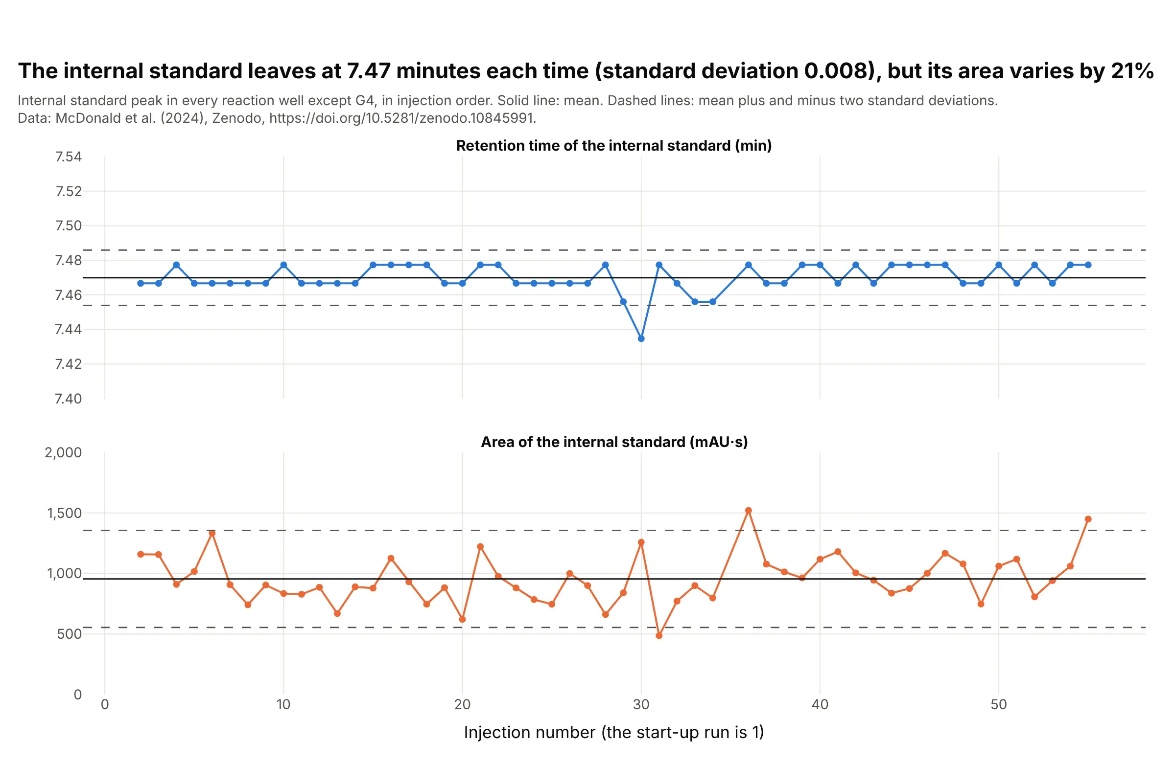
A lab injects the same reference over and over and charts where its peak lands, so a drifting pump or column shows before it spoils a result. Here the internal standard leaves at 7.47 minutes in all 53 injections with a standard deviation of 0.008 minutes, which is less than the 0.011 minutes between two data points, while its area varies by 21% of its mean. The mean and two-standard-deviation lines are those of a control chart, and a Levey-Jennings chart is the same idea for clinical laboratory controls. Data: McDonald et al. (2024), 54 wells without G4, whose internal standard is hidden by a large peak at 7.27 minutes.
Tip: chart the retention time and the area separately, because the first checks the column and the pump and the second checks the injection.
Get the data from the Zenodo record doi 10.5281/zenodo.10845991 (McDonald et al. 2024), reaction_set_1.zip: the PDA exportsPDA_Data_002.txt to PDA_Data_055.txt (the file number is the injection order; take the 254 nm column, divided by 1,000).For each run except PDA_Data_036 (well G4), find the internal standard peak between 7.2 and 7.8 minutes and integrate itfrom 7.00 to 7.95 minutes above a straight baseline. Make a plotly figure with two stacked line charts against injectionnumber, the retention time and the area, each with the mean as a solid line and mean plus and minus two standarddeviations as dashed lines.
5. Peak purity from the spectrum
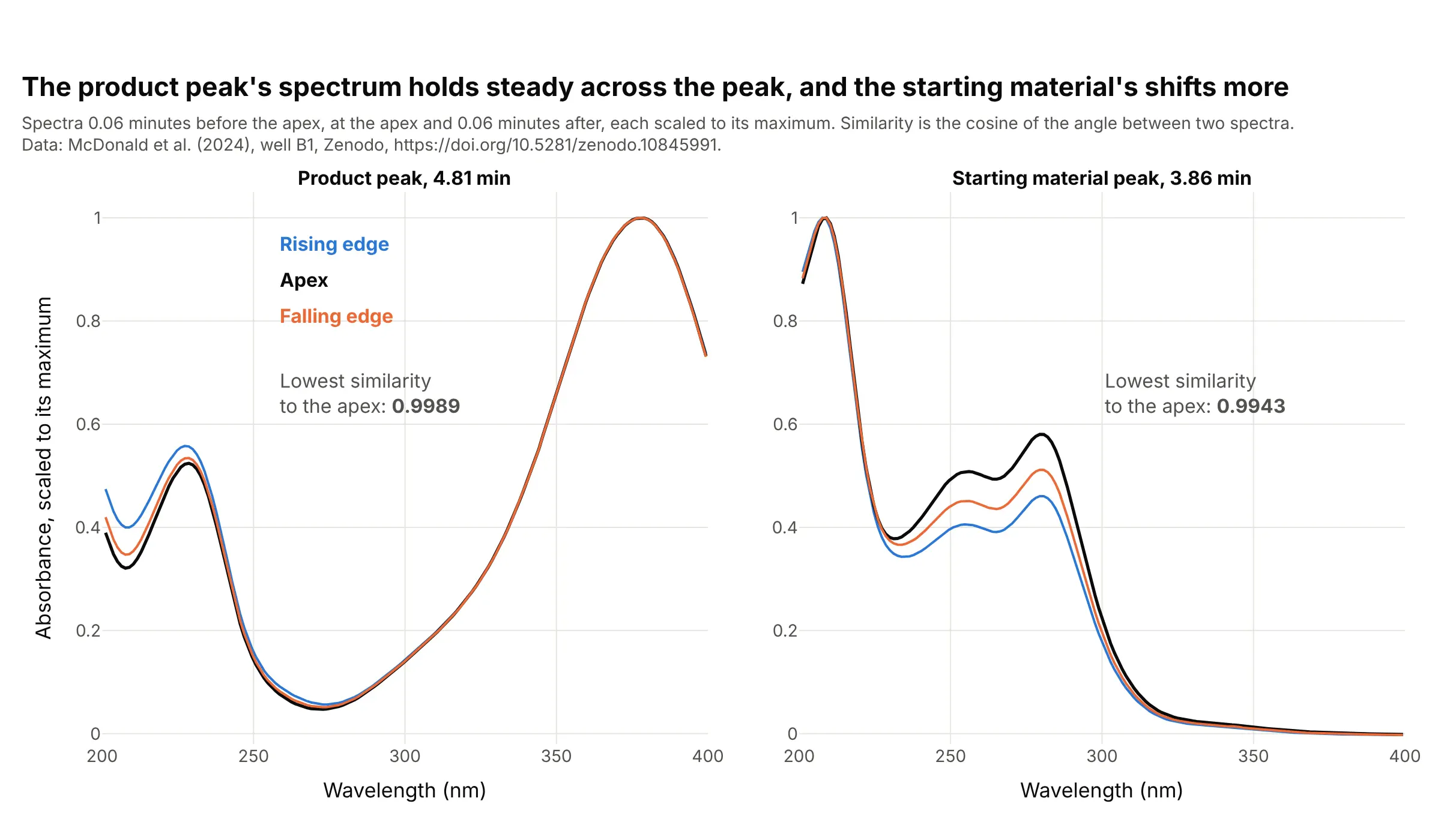
A photodiode-array detector records a spectrum at every moment, so one peak can be checked for a hidden compound: a pure peak has the same spectrum on its rising edge, at its apex and on its falling edge. For the product the cosine similarity between the apex and the other two spectra is at least 0.9989, and for the starting material it is 0.9943, so its shape changes more. That is not proof of a second compound, since labs set their own thresholds and a very tall peak can distort a spectrum. Data: McDonald et al. (2024), well B1, 200 to 400 nm.
Tip: scale each spectrum to its own maximum before you compare shapes, and write the similarity on the chart.
Get the data from the Zenodo record doi 10.5281/zenodo.10845991 (McDonald et al. 2024), reaction_set_1.zip, filePDA_Data_007.txt (well B1; a [PDA 3D] section whose header row holds wavelengths multiplied by 100 and whose rowshold the time in minutes followed by the absorbance in micro-absorbance units, an assumption, at each wavelength).Take the spectra 0.06 minutes before the apex, at the apex and 0.06 minutes after it for the peaks at 4.81 and 3.86 minutes,200 to 400 nm. Scale each to its maximum and make two plotly panels of the three curves, with the lowest cosine similarity tothe apex spectrum written on each.
6. Impurity profiling: one product, three electrolytes
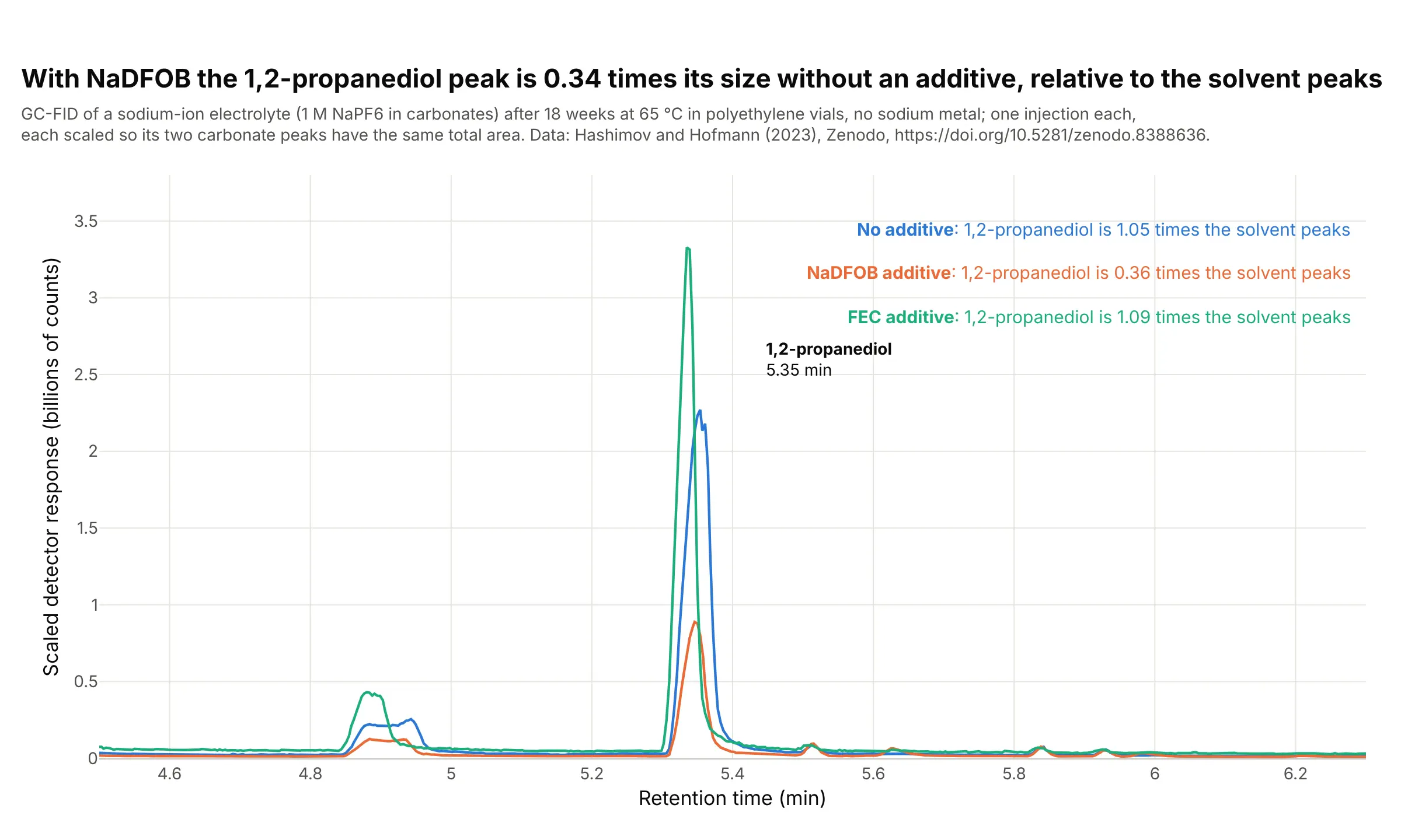
Impurity profiling asks how much of each unwanted compound a batch contains, and a common way is to scale runs to the main peaks. After 18 weeks at 65 °C in polyethylene vials, the 1,2-propanediol peak is 1.05 times the area of the two carbonate solvent peaks in an electrolyte with no additive, 0.36 with the additive NaDFOB and 1.09 with FEC, so the NaDFOB run has 0.34 times the relative amount. This is one injection per sample, and a flame ionization detector responds differently to each compound, so the ratios compare runs and are not mass ratios. Data: Hashimov and Hofmann (2023), samples a5, b5 and c5.
Tip: scale each run so the main peaks have the same area, and say in the subtitle what you divided by.
Get the data from the Zenodo record doi 10.5281/zenodo.8388636 (Hashimov and Hofmann 2023), file GC_data.xlsx, sheetsMH_a5_18weeks_CHR, MH_b5_18weeks_CHR and MH_c5_18weeks_CHR (columns ret in minutes and counts).Integrate 1,2-propanediol (5.22 to 5.46 minutes) and the ethylene and propylene carbonate peaks (7.55 to 7.80 and 7.80 to8.15 minutes) above a straight baseline, scale each run so the two carbonate peaks have the same total area, and make aplotly line chart of the three runs from 4.5 to 6.3 minutes, colored by additive (none, NaDFOB, FEC), with the ratio of1,2-propanediol to the carbonates written in each label.
7. A peak that is missing is a result
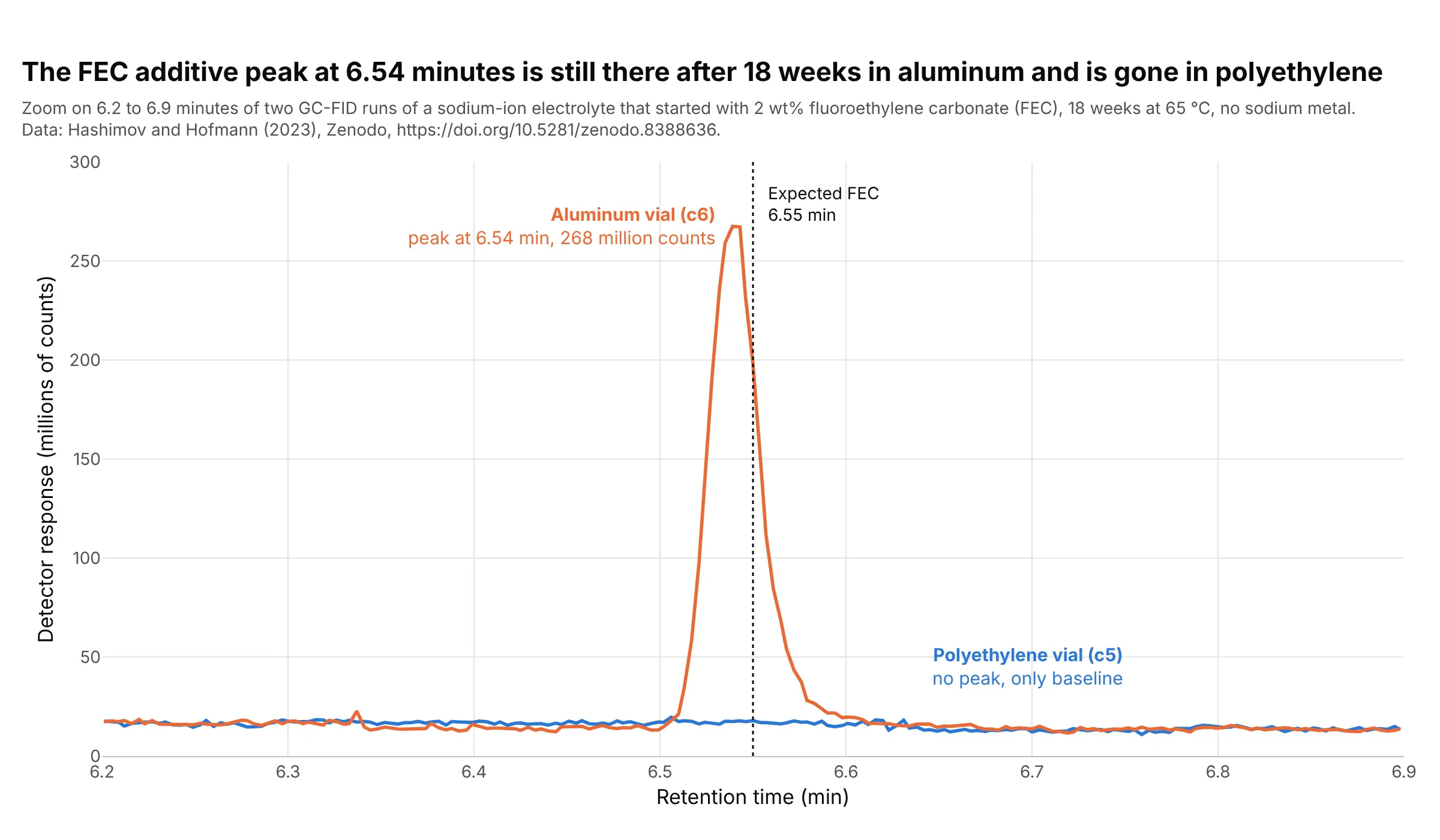
A reference retention time turns a flat stretch of a trace into an answer. The additive fluoroethylene carbonate (FEC) leaves the column at 6.55 minutes in the paper's table, and after 18 weeks at 65 °C it still gives a peak of 268 million counts in the aluminum vial and nothing in the polyethylene vial, which the paper reports as no longer detectable. The aluminum sample is the more concentrated one, so the heights are not compared. Data: Hashimov and Hofmann (2023), samples c5 and c6.
Tip: mark the expected retention time with a dotted line, so a missing peak is a visible gap and not an overlooked one.
Get the data from the Zenodo record doi 10.5281/zenodo.8388636 (Hashimov and Hofmann 2023), file GC_data.xlsx, sheetsMH_c5_18weeks_CHR and MH_c6_18weeks_CHR (columns ret in minutes and counts).Make a plotly line chart of both runs from 6.2 to 6.9 minutes in millions of counts, with a dotted vertical line at 6.55minutes labeled "Expected FEC", the aluminum run (c6) in orange and the polyethylene run (c5) in blue, and a label on thepeak with its height.
FAQ
Options to customize
- mode="lines" draws the trace as a thin line without markers, the standard look for a chromatogram. Reference: go.Scatter.
- fill="toself" shades a peak when the trace's x and y run along the curve and back along the baseline, and fill="tozeroy" shades down to zero when the baseline is flat.
- add_annotation labels each peak with its retention time and area, and showarrow=False with yshift keeps the label above the apex. Reference: annotations.
- add_vline marks a reference retention time, such as the time a standard elutes, so a missing peak is a visible gap.
- xaxis.range zooms into one stretch, such as the baseline or a pair of close peaks, and xaxis.dtick sets the minute ticks.
- make_subplots(shared_xaxes=True) stacks a chromatogram with a second view on the same time axis, such as a control chart of an internal standard. Reference: subplots.
- go.Heatmap draws time against wavelength for photodiode-array data, and zmax clips the solvent front so the peaks stay visible. Reference: go.Heatmap.
- hovertemplate shows the retention time and the response on hover, and hoverinfo="skip" turns hover off for the shaded areas.
- go.Scattergl is the WebGL version of the line trace, worth testing for many overlaid runs on a machine with a graphics card.
- xaxis.rangeslider adds a slider under the chart to scroll along a long run.