Chris Parmer

November 9, 2026

Spectrograms - A Complete Guide

TL;DR

A spectrogram shows how the frequencies in a signal change over time: time on the x axis, frequency on the y axis (often logarithmic), and the power at each time and frequency as color, almost always in decibels (dB).
Spectrograms are also known as sonograms or sonographs, and, for speech, voiceprints or voicegrams. A plot of the short-time Fourier transform (STFT) is a spectrogram, and a spectral waterfall plot draws the same data as stacked spectra. They are similar to heatmaps, which they are built from, and to Bode plots, which show frequency without time.
Acousticians, seismologists, physicists, sleep scientists and vibration engineers read them for the shapes a waveform hides: tones are horizontal lines, harmonics are stacks of lines, chirps are sloped lines, impacts are vertical lines, and noise is a smear.
You can make a spectrogram with Plotly from scipy.signal.spectrogram and a go.Heatmap, with the waveform in a row above on a shared time axis. The code is below.

What is a spectrogram?

Spectrograms look like this:

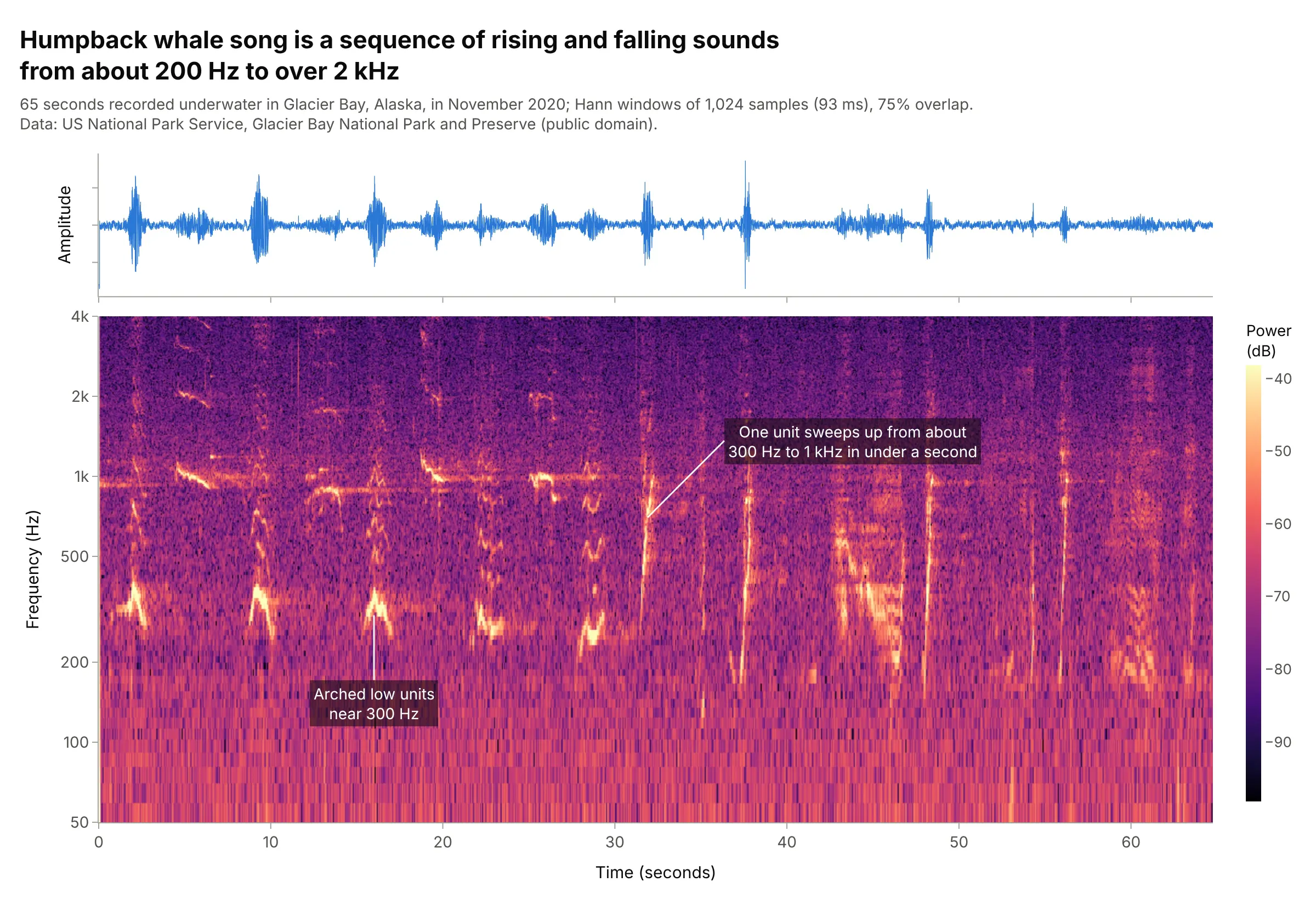
Spectrogram of 65 seconds of humpback whale song recorded underwater in Glacier Bay, Alaska, with the waveform above on a shared time axis: bright arched units near 300 Hz repeat through the first 30 seconds, fainter marks reach above 2 kHz, and one unit at 32 seconds sweeps up from about 300 Hz to 1 kHz in under a second

Data: US National Park Service, Glacier Bay National Park and Preserve (public domain), humpback whale song recorded in November 2020.

How do you read a spectrogram? In the example above, notice these things:

The waveform on top only says when the sound is loud. The spectrogram below it splits the same 65 seconds into frequencies, so each sound in the song gets a shape: arches near 300 Hz, sweeps, and faint marks above 2 kHz.
Each column is the spectrum of a short slice of the recording (here 93 milliseconds), and each cell's color is the power at that time and frequency, from dark (quiet) to bright yellow (loud).
The color is in decibels and covers 60 dB, a factor of a million in power, so quiet harmonics and the background noise show next to the loudest sounds.
The frequency axis is logarithmic, so 100 to 200 Hz gets as much height as 1 to 2 kHz. The unit at 32 seconds is a sloped line, a pitch that rises from about 300 Hz to 1 kHz in under a second.

It's often used for charts like these:

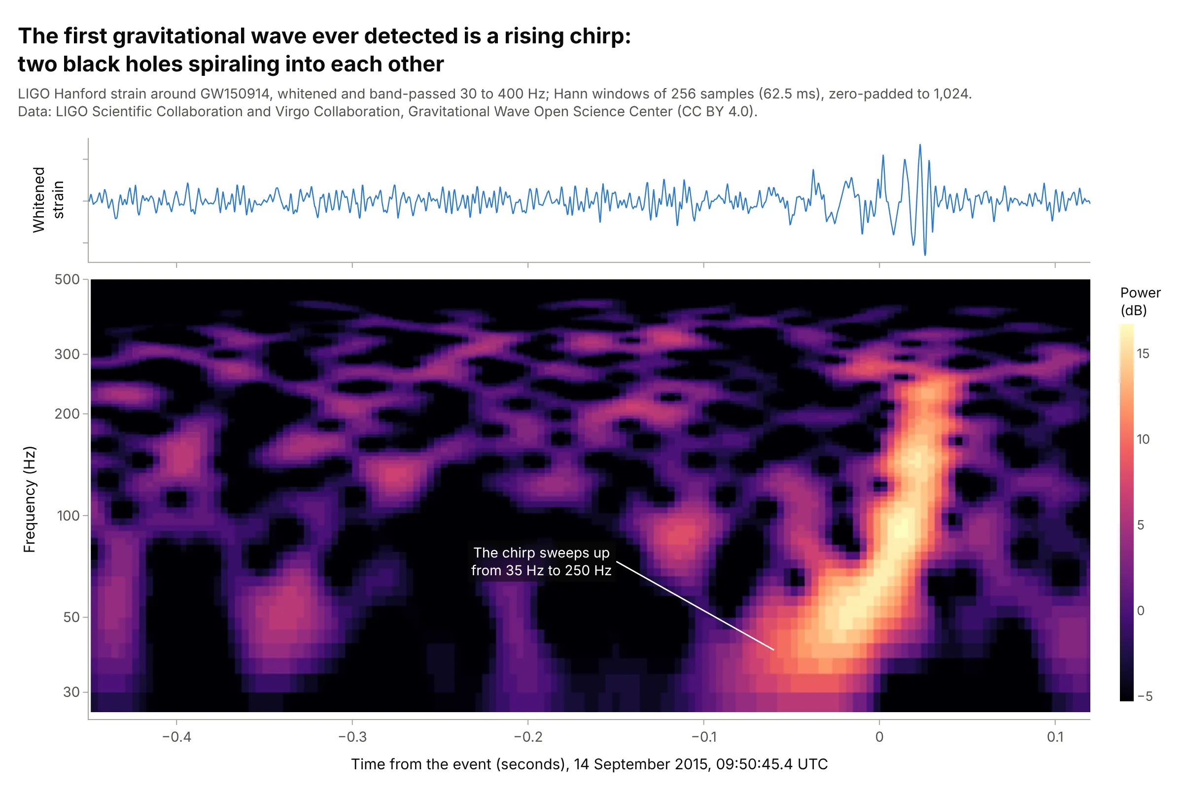
Spectrogram of the LIGO Hanford detector's whitened strain around GW150914 with the whitened waveform above: a bright band sweeps up from about 35 Hz at 0.1 seconds before the event to about 250 Hz just after it, on a log frequency axis from 25 to 500 Hz

Physics. On September 14, 2015, the LIGO detectors recorded the first gravitational wave ever seen, from two black holes of about 36 and 29 times the mass of the Sun merging, and its spectrogram is a chirp sweeping up from 35 to 250 Hz. Data: LIGO Scientific Collaboration and Virgo Collaboration, Gravitational Wave Open Science Center (CC BY 4.0); Abbott et al. (2016).

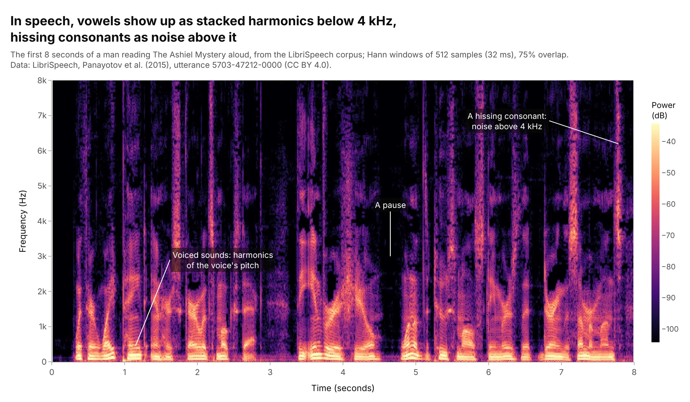
Spectrogram of the first 8 seconds of a man reading a novel aloud, linear frequency axis from 0 to 8 kHz: voiced sounds are stacks of closely spaced harmonics below about 3 kHz, a pause at 4.6 seconds is blank, and a hissing consonant near 7.8 seconds is a vertical smear above 4 kHz

Speech. Vowels show up as stacks of harmonics of the voice's pitch shaped into bands, hissing consonants like "s" as noise above 4 kHz, and pauses as blank columns, which is why phoneticians learn to read words off a spectrogram. Data: LibriSpeech (CC BY 4.0), utterance 5703-47212-0000.

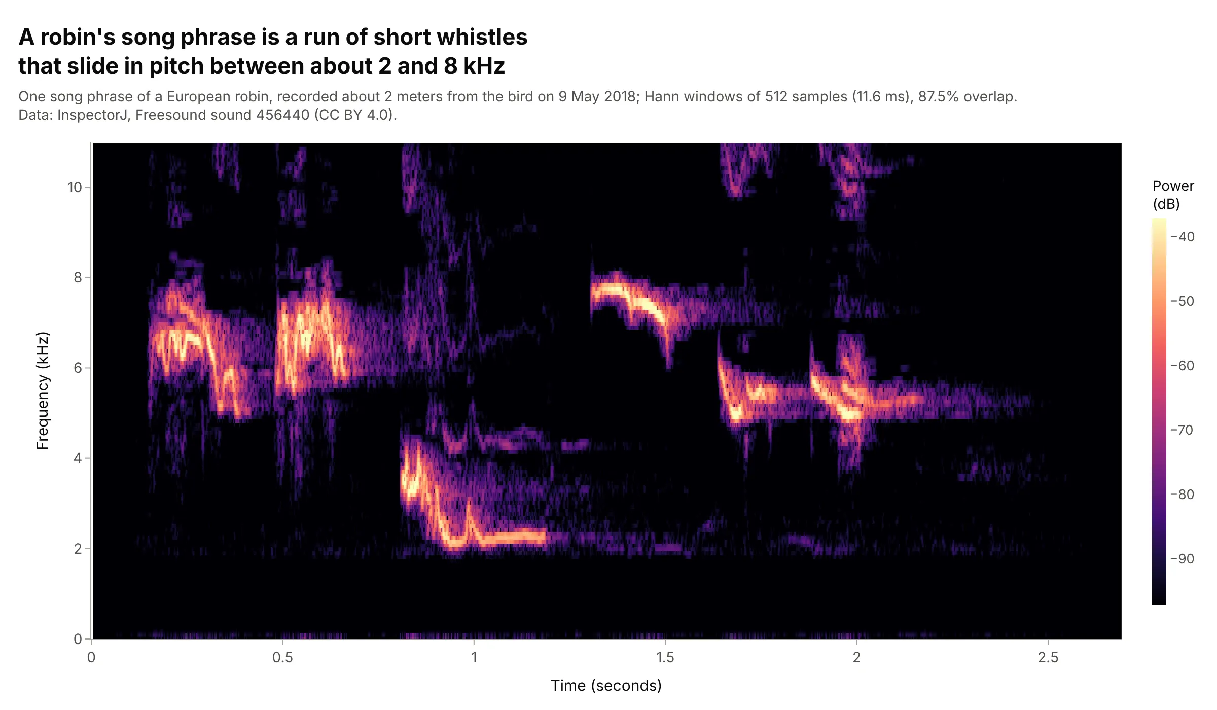
Spectrogram of a European robin's song phrase lasting 2.7 seconds, linear frequency axis from 0 to 11 kHz: a run of short whistles that slide between about 2 and 8 kHz, two high notes near 7 kHz at the start, a falling note from 4 to 2 kHz at 0.9 seconds, and notes near 7.5 and 5.5 kHz after 1.3 seconds

Bird song. Ornithologists compare songs by their shapes in time and frequency, and a robin's phrase is a run of short whistles that slide between about 2 and 8 kHz. Data: InspectorJ, Freesound sound 456440 (CC BY 4.0).

How to read a spectrogram

A spectrogram assumes three ideas that people who work with signals use every day and most other readers have never needed: how the short-time Fourier transform cuts a signal into slices, how the length of a slice trades time detail for frequency detail, and why the color is in decibels. Once those are clear, the shapes on the chart are easy to read.

The short-time Fourier transform (STFT)

A Fourier transform turns a stretch of signal into its spectrum: how much power the signal has at each frequency. A spectrum of a whole recording loses the timing, so the short-time Fourier transform takes the spectrum of one short window at a time, slides the window along, and stacks the spectra side by side. Each window is tapered at both ends (the Hann window is the usual choice) so the cut edges don't add false frequencies, and windows usually overlap by 50% to 90% so nothing falls between them:

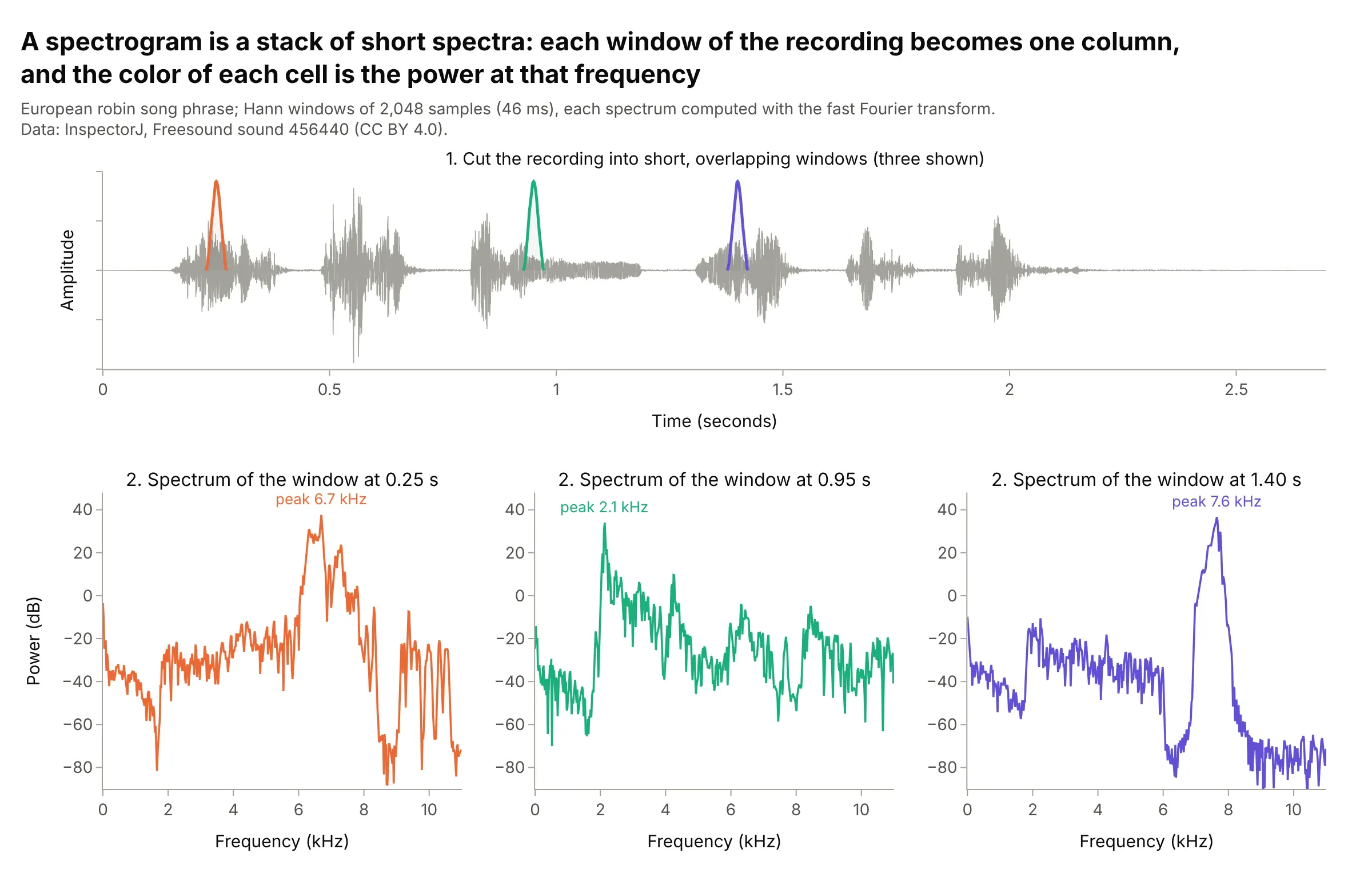
The robin's waveform with three bell-shaped Hann windows at 0.25, 0.95 and 1.40 seconds, and below it the power spectrum of each window: the first peaks near 6.7 kHz, the second near 2.1 kHz and the third near 7.6 kHz

Data: InspectorJ, Freesound sound 456440 (CC BY 4.0).

Each spectrum becomes one column of the spectrogram, with its power turned into color. The spectrogram is the squared magnitude of the STFT, which is why the two names are used for the same chart.

Window length: time detail or frequency detail

The window length sets what you can see. A window of N samples at a sample rate of fs gives frequency bins fs / N apart, so a longer window separates frequencies more finely, but it also averages over a longer time and smears anything that happens quickly. You can't have both, and this test signal shows why:

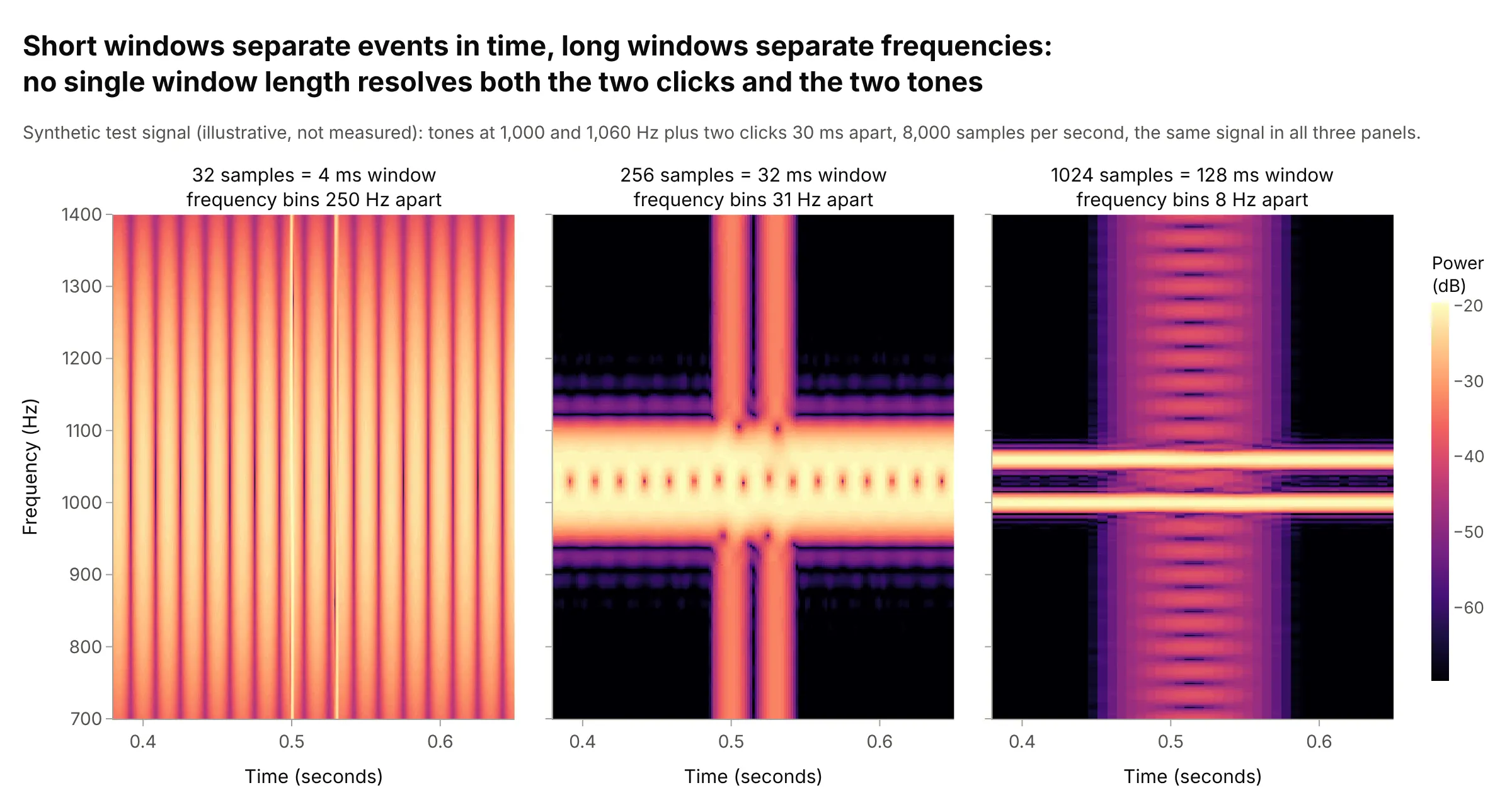
Three spectrograms of the same synthetic signal, two steady tones at 1,000 and 1,060 Hz and two clicks 30 milliseconds apart: with a 4 ms window the clicks are two thin vertical lines but the tones merge into one band; with a 32 ms window the clicks are still separate and the tones still merged; with a 128 ms window the tones are two separate horizontal lines and the clicks have smeared into one blob

Data: a synthetic test signal (illustrative, not measured), described on the image.

In practice, pick the window from the features you care about: a few milliseconds for clicks, speech consonants and machine impacts, tens of milliseconds for speech and bird song, and seconds or minutes for whale calls, earthquakes and sleep. The examples in this guide use windows from 5.3 milliseconds to 205 seconds. Overlap and zero-padding (computing the transform with extra zeros, nfft in scipy) make the picture smoother but don't add real resolution.

Decibels

Power in signals spans a huge range: the loudest cells of the whale song above (the top 0.1%) are about 40 dB, 10,000 times, stronger than the typical (median) cell. On a linear color scale only the loudest few cells show, so spectrograms color by decibels, 10 × log10 of the power, where every factor of 10 in power is the same 10 dB step of color:

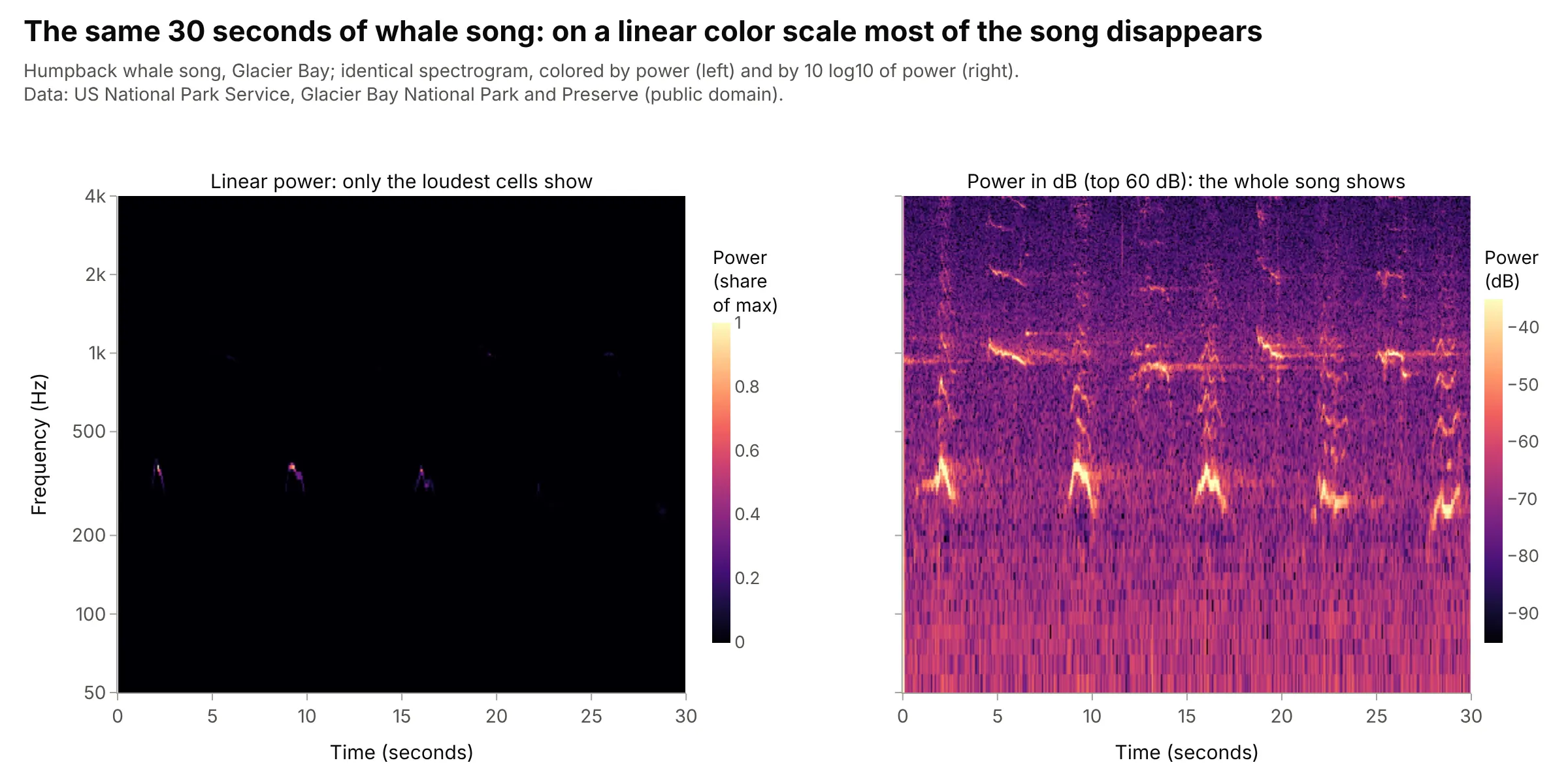
The same 30 seconds of humpback whale song colored two ways: on a linear power scale only three small bright marks near 300 Hz are visible and the rest is black; in dB with a 60 dB range every unit, its harmonics and the background noise are visible

Data: US National Park Service, Glacier Bay National Park and Preserve (public domain).

Two choices matter. First, the range: clip the colors to the top 40 to 80 dB (60 dB is a good start), because a few near-silent cells can otherwise stretch the scale and wash out everything else. Second, the reference: unless the sensor is calibrated, the dB values are relative (to the loudest cell, or to 1 unit squared per Hz), so say so. A perceptually uniform dark-to-bright colorscale such as Magma, Inferno or Viridis reads correctly in grayscale and for colorblind readers.

Linear or log frequency

A linear frequency axis keeps harmonics evenly spaced, which makes a fundamental and its multiples easy to spot (the engine example below). A log axis gives every doubling of frequency, an octave, the same height, so it suits music, hearing and signals that span several decades, like a seismogram from 0.005 to 4 Hz. Speech scientists traditionally use linear 0 to 8 kHz; acousticians and musicians use log; machine-learning models for audio often use a mel scale, which is roughly linear below 1 kHz and logarithmic above.

Reading the shapes

Most features fall into a few shapes:

Horizontal line: a steady tone, like an engine, a hum or a held note.
Stack of evenly spaced lines: a tone with harmonics at 2, 3, 4 ... times its frequency, which is what voices, instruments and rotating machines make.
Sloped or curved line: a pitch that changes, a chirp or a sweep, like the LIGO signal and the whale's units.
Vertical line: a click or impact, which has power at every frequency for an instant.
Smear or band: noise, like wind, a hissing consonant or the ocean's background.

A short history

The spectrogram was invented at Bell Telephone Laboratories during the 1940s to make speech visible. Three Bell Labs engineers, Koenig, Dunn and Lacy, described their "sound spectrograph", which they credit to their colleague Ralph K. Potter, in The Journal of the Acoustical Society of America in July 1946 (scan). It recorded "the last 2.4 seconds of signal" on a loop of magnetic tape and drew the analysis onto paper with a recording stylus on a linear frequency scale covering 3,500 cycles per second, with a choice of "the narrow (45-cycle) analyzing filter" or "the wide (300-cycle) filter"; the paper already showed spectrograms of speech, music and bird songs. This is that layout, redrawn on modern speech:

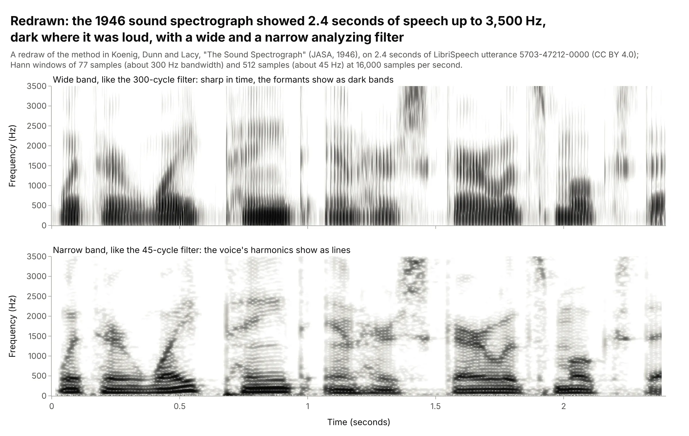
Two gray-scale spectrograms of 2.4 seconds of read speech from 0 to 3,500 Hz, dark where the sound is loud: with a wide-band 300 Hz analysis the time detail is sharp and the vowel formants show as dark bands; with a narrow-band 45 Hz analysis the individual harmonics of the voice show as closely spaced horizontal lines

Data: a redraw of the method in Koenig, Dunn and Lacy (1946) on LibriSpeech utterance 5703-47212-0000 (CC BY 4.0), with Hann windows whose bandwidths match the two filters.

The wide and narrow filters are the window length trade-off from the section above, 80 years before most of us met it in scipy: phoneticians still call them wide-band and narrow-band spectrograms.

Alternatives to a spectrogram

Here's the same robin song drawn six ways. Some are better for the question, some worse, some just different:

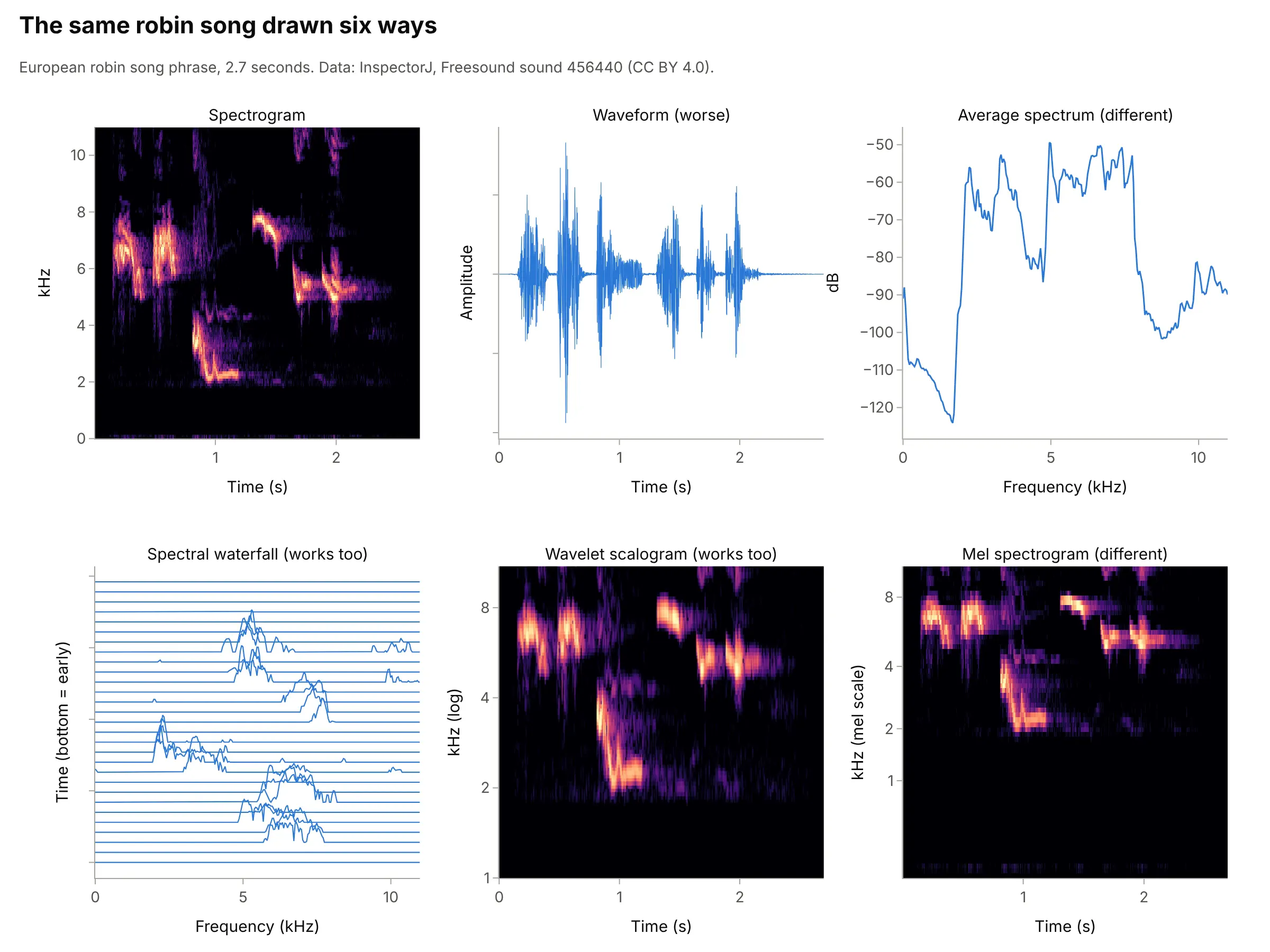
Six charts of the same 2.7-second robin song: a spectrogram with the notes between 2 and 8 kHz; the waveform, which shows only when the bird sang; the average spectrum, a single curve with power between 2 and 8 kHz and no timing; a spectral waterfall of offset spectra, one every 0.09 seconds; a wavelet scalogram on a log frequency axis with similar shapes; and a mel spectrogram with the high notes squeezed together

Waveform (worse). It shows when the bird sang and how loud, but not the pitch of anything. It's still worth drawing above the spectrogram, on a shared time axis, as in the main example.
Average spectrum (different). One spectrum of the whole recording, usually estimated with Welch's method, shows which frequencies are present (here 2 to 8 kHz) but not when. Use it, or a Bode plot for a system's response, when the signal doesn't change over time.
Spectral waterfall (works too). Stacking the spectra as offset lines, or as a 3D surface, is the "waterfall plot" of vibration and radio engineering. It shows peak heights exactly but hides lines behind each other; a ridgeline plot is the same idea for distributions.
Wavelet scalogram (works too). A continuous wavelet transform uses short windows at high frequencies and long ones at low frequencies, so it sidesteps part of the window trade-off. It costs more to compute and its frequency resolution varies with frequency.
Mel spectrogram (different). The same power pooled into bands spaced like human pitch perception. It's the standard input to speech and audio machine-learning models, but its axis is harder to read in hertz.

A spectrogram is a heatmap with time and frequency as its axes, so the heatmap guide's advice on color scales applies, and a line chart of the power in one band over time (like the sleep example's slow waves) is often the clearest summary of one feature. The strip chart guide draws the same Kamchatka seismogram used below as a classic recorder trace.

How to make a spectrogram

With AI

ChatGPT, Claude Code, GitHub Copilot, Cursor and other AI tools are excellent at writing Plotly code. Name Plotly in the prompt, and say the sample rate, the window length and the frequency range you care about:

Make a plotly spectrogram of humpback.wav (mono, 11,025 samples per second).

- Compute it with scipy.signal.spectrogram: Hann windows of 1,024 samples, 75% overlap.
- Convert power to dB (10 * log10) and clip the color range to the top 60 dB, colorscale Magma.
- Show 50 Hz to 4 kHz on a log y axis labeled in Hz, time in seconds on x.
- Put the waveform in a row above with make_subplots(rows=2, shared_xaxes=True).

With Plotly Studio

Plotly Studio is a desktop app where you point an AI at a dataset and it builds charts and a Dash app around your questions. Ask for a spectrogram the same way:

Show a spectrogram of this vibration recording (12,000 samples per second) in dB, with the waveform above on a shared time axis, a slider for the window length from 64 to 4,096 samples, and a dropdown to switch the frequency axis between linear and log.

Make a spectrogram in Python or JavaScript

This is the code AI tools write under the hood. Plotly has no dedicated spectrogram trace, so a spectrogram is a go.Heatmap of the output of scipy.signal.spectrogram, with the waveform as a go.Scatter in a row above. This helper returns a go.Figure, and every example in this guide builds on the same idea:

import numpy as np
import plotly.graph_objects as go
from plotly.subplots import make_subplots
from scipy import signal
from scipy.io import wavfile


def spectrogram_figure(x, fs, nperseg=1024, overlap=0.75, fmin=50, fmax=None, db_range=60, log_y=True):
    """A spectrogram in Plotly: the waveform on top, power in dB below, one shared time axis."""
    f, t, Sxx = signal.spectrogram(x, fs, window="hann", nperseg=nperseg, noverlap=int(nperseg * overlap))
    keep = (f >= fmin) & (f <= (fmax or fs / 2))
    S_db = 10 * np.log10(Sxx[keep] + 1e-20)             # power in decibels
    top = np.percentile(S_db, 99.9)                     # clip the color range to the top db_range dB

    fig = make_subplots(rows=2, cols=1, shared_xaxes=True, row_heights=[0.25, 0.75], vertical_spacing=0.03)
    fig.add_trace(go.Scatter(x=np.arange(len(x)) / fs, y=x, mode="lines", line_width=0.6), row=1, col=1)
    fig.add_trace(go.Heatmap(x=t, y=f[keep], z=S_db, zmin=top - db_range, zmax=top, colorscale="Magma",
                             colorbar=dict(title="Power (dB)", len=0.75, y=0.375)), row=2, col=1)
    fig.update_yaxes(title_text="Frequency (Hz)", type="log" if log_y else "linear", row=2, col=1)
    fig.update_xaxes(title_text="Time (seconds)", row=2, col=1)
    fig.update_layout(template="simple_white", showlegend=False)
    return fig


fs, x = wavfile.read("humpback.wav")                   # any mono WAV file
fig = spectrogram_figure(x.astype(float), fs, nperseg=1024, fmin=50, fmax=4000)
fig.show()

scipy.signal.spectrogram is now marked as a legacy function; scipy.signal.ShortTimeFFT is its newer replacement and has a spectrogram method that returns the same array. For sensor data that isn't audio, read it with pandas or the field's own library (ObsPy for seismograms, MNE or pyEDFlib for EEG, h5py for LIGO's files) and pass the samples and the sample rate. For a log y axis, drop the 0 Hz row, since a log axis can't show zero.

In JavaScript, plotly.js draws the same heatmap. This example computes a small STFT in the browser for a test signal:

<div id="chart"></div>
<script src="https://cdn.plot.ly/plotly-4.1.1.min.js"></script>
<script>
  // A test signal: a chirp rising from 200 to 3,000 Hz over 2 seconds, sampled at 8,000 Hz
  const fs = 8000, n = 2 * fs;
  const x = Array.from({length: n}, (_, i) => { const t = i / fs; return Math.sin(2 * Math.PI * (200 * t + 700 * t * t)); });

  // Short-time Fourier transform: Hann windows of 256 samples, hop 64, power in dB
  const N = 256, hop = 64, hann = Array.from({length: N}, (_, i) => 0.5 - 0.5 * Math.cos(2 * Math.PI * i / N));
  const freqs = Array.from({length: N / 2}, (_, k) => k * fs / N), times = [], z = freqs.map(() => []);
  for (let start = 0; start + N <= n; start += hop) {
    times.push((start + N / 2) / fs);
    for (let k = 0; k < N / 2; k++) {
      let re = 0, im = 0;
      for (let i = 0; i < N; i++) { const a = 2 * Math.PI * k * i / N, v = x[start + i] * hann[i]; re += v * Math.cos(a); im -= v * Math.sin(a); }
      z[k].push(10 * Math.log10(re * re + im * im + 1e-12));
    }
  }
  const peak = Math.max(...z.flat());
  Plotly.newPlot("chart", [{type: "heatmap", x: times, y: freqs, z: z, zmin: peak - 60, zmax: peak,
                            colorscale: "Viridis", colorbar: {title: {text: "Power (dB)"}}}], {
    width: 900, height: 500,
    xaxis: {title: {text: "Time (seconds)"}},
    yaxis: {title: {text: "Frequency (Hz)"}}
  });
</script>

In a real app, compute the spectrogram on the server (or with a fast Fourier transform library) and send plotly.js the dB array.

Share it

Every Plotly chart has a Share chart button (the cloud icon in its toolbar) that uploads it to Plotly Cloud and gives you a link. Only you can see it until you change its visibility.

For a live app, put the chart in a Dash app and publish it with the Plotly Cloud CLI. Coding agents can run these commands for you:

pip install "dash[cloud]"
plotly user login
plotly app publish

If your data has to stay in your own cloud or data center, publish to Dash Enterprise instead.

Dos and don'ts

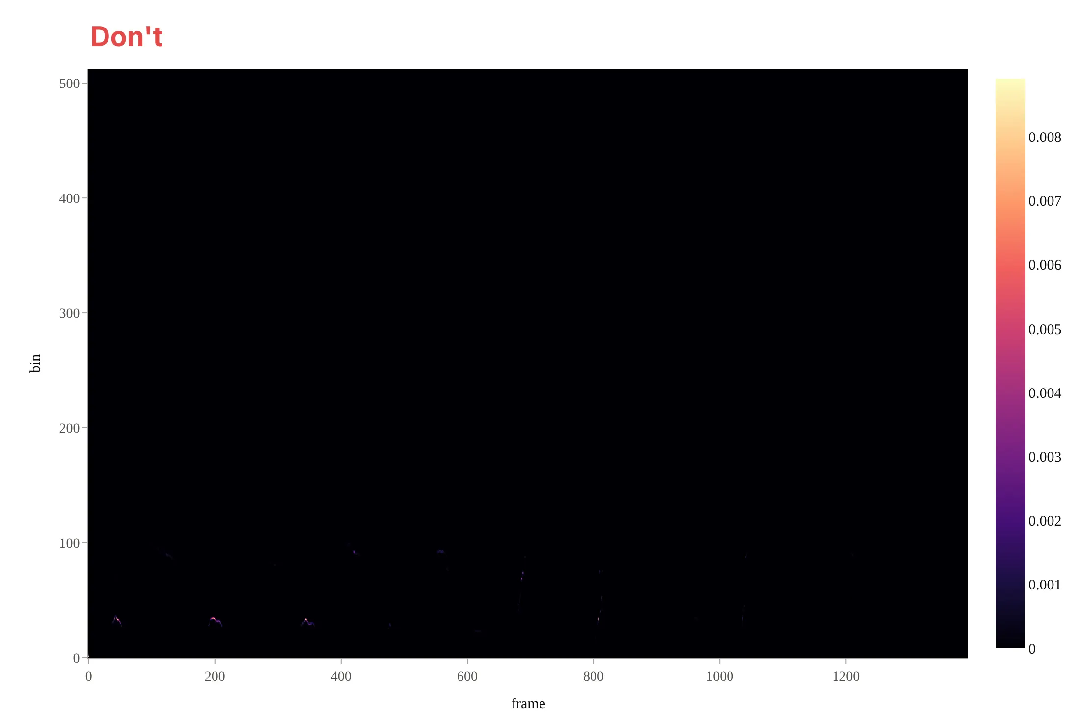
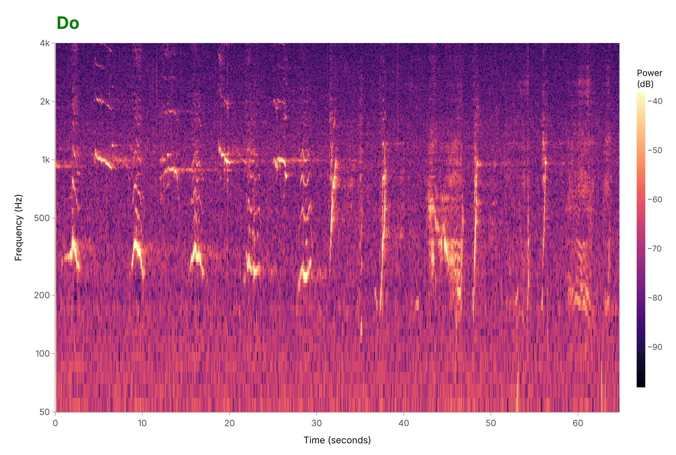
Most spectrograms that are hard to read skip the steps between the raw array and the chart: decibels, units on the axes and a frequency range that fits the signal. Here is the whale song from the top of the guide both ways, with the same Magma colorscale.

Don't color by linear power (only three loud marks show), label the axes with array indices ("frame" and "bin") instead of seconds and hertz, show the full 0 Hz to 5.5 kHz range on a linear axis when the song lives between 200 Hz and 2 kHz, leave the colorbar without a title or unit, and keep a default serif font:

The whale song spectrogram colored by linear power: almost entirely black with three faint marks near the bottom, axes titled frame and bin with ticks up to 1,400 and 500, an untitled colorbar from 0 to 0.003, and a serif font

Do color by dB with the range clipped to the top 60 dB, show 50 Hz to 4 kHz on a log axis in Hz, put time in seconds, and title the colorbar with its unit:

The same whale song in dB on a log frequency axis from 50 Hz to 4 kHz and time from 0 to 65 seconds, with a colorbar titled Power (dB): every unit, sweep and harmonic is visible

Checklist

Color by power in dB and clip the range (40 to 80 dB), with a dark-to-bright, perceptually uniform colorscale.
Label the axes in seconds and hertz, and say in the subtitle what the window length and overlap were.
Choose the window length for the features you want (short for clicks, long for tones), and say on the chart which you chose.
Use a log frequency axis for signals that span several octaves, and a linear one when you need to see evenly spaced harmonics.
Draw the waveform, or the event markers, in a row above with a shared time axis.

Don't

Use a rainbow or diverging colorscale for power; it invents edges where the power changes smoothly.
Compare dB values between recordings that weren't calibrated the same way.
Read frequencies above half the sample rate (the Nyquist frequency): they aren't there, and anything that was has been folded down unless the recording was filtered first.
Trust a frequency or a time more precisely than the window allows (bins are fs / N apart; times blur over N / fs seconds).

Options to customize

A spectrogram in Plotly is a go.Heatmap of an STFT, so these are the options that matter most. The full lists are in the heatmap trace reference, the heatmap documentation and the scipy.signal.spectrogram reference.

nperseg (window length) and noverlap: the time and frequency resolution; start at 20 to 50 ms for sound and 75% overlap.
window="hann": the taper; scipy's legacy spectrogram defaults to a Tukey window, and Hann is the common choice.
nfft: zero-padding for a smoother frequency axis without new resolution.
z=10 * np.log10(Sxx): power in dB; use mode="magnitude" and 20 × log10 if you want amplitude.
zmin and zmax: the clipped color range, usually the top 40 to 80 dB.
colorscale="Magma": a perceptually uniform dark-to-bright scale (Inferno and Viridis work too in Python; plotly.js has Viridis and Cividis built in).
fig.update_yaxes(type="log"): a log frequency axis; set tickvals and ticktext for 50, 100, 1k ... or note names.
make_subplots(rows=2, shared_xaxes=True, row_heights=[0.25, 0.75]): the waveform or an event track above the spectrogram, zooming together.
hovertemplate="%{x:.2f} s<br>%{y:.0f} Hz<br>%{z:.0f} dB": readable hover labels with units.
zsmooth="best": smooth interpolation between cells for presentation; leave it off when you need to see the bins.

More spectrogram examples

Six more spectrograms built from real public data, each with its source, the technique that makes it work and a prompt to rebuild it. They run from a millisecond-scale bearing fault to an hour of whale song and a whole night of sleep.

1. An hour of blue and fin whale song in Monterey Bay

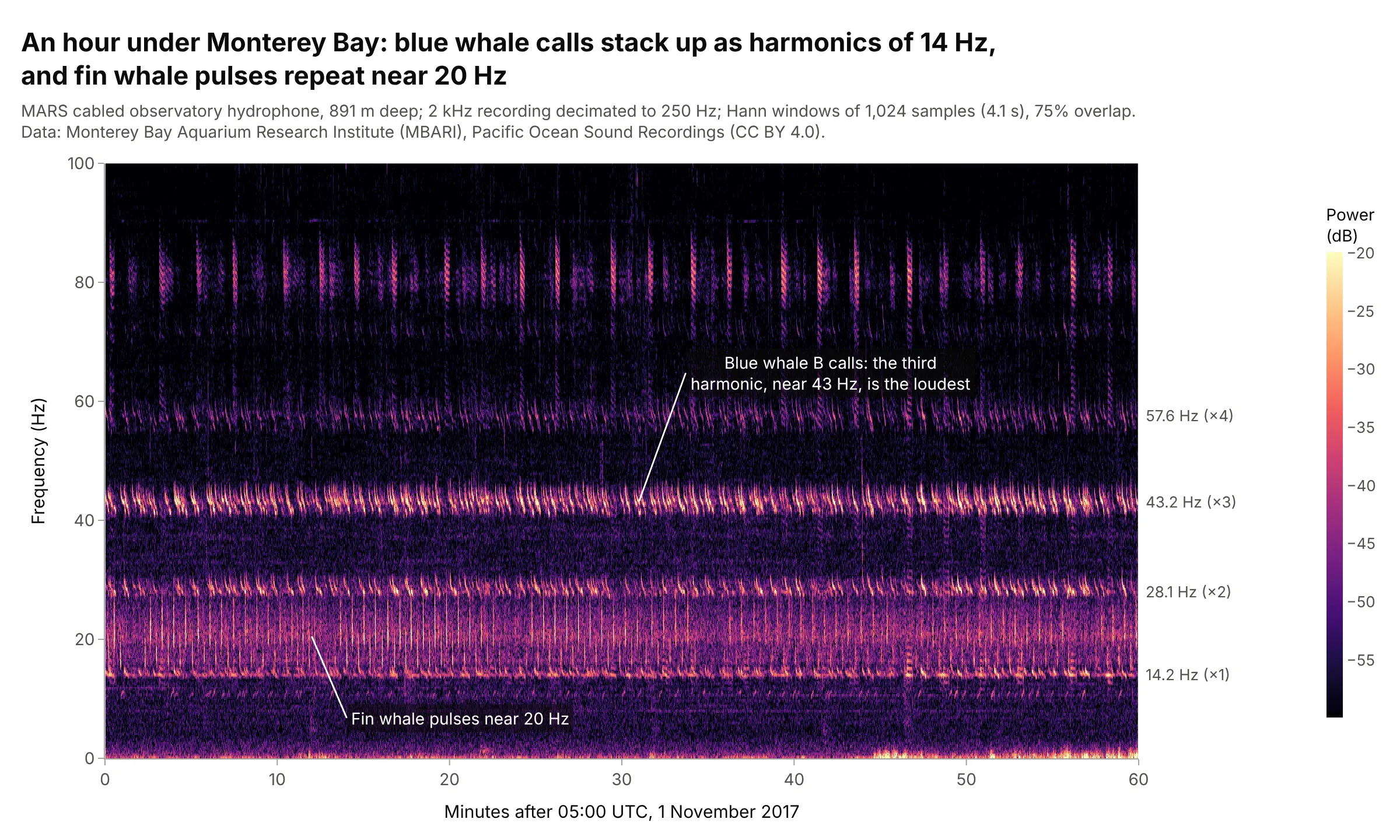
Spectrogram of one hour of deep-ocean sound in Monterey Bay, 0 to 100 Hz: blue whale B calls form repeating marks at 14.2, 28.1, 43.2 and 57.6 Hz, brightest at 43 Hz, and fin whale pulses are short vertical marks repeating near 20 Hz

A hydrophone 891 m deep recorded both of the largest whales singing in one hour. Blue whale B calls are stacks of harmonics of about 14 Hz, with the third, near 43 Hz, the loudest, and fin whale pulses repeat near 20 Hz, which is why ocean acousticians use 4-second windows and a linear 0 to 100 Hz axis for them. Data: MBARI Pacific Ocean Sound Recordings (CC BY 4.0), 1 November 2017, 05:00 to 06:00 UTC.

Tip: label the harmonics on the right edge, so readers can check that the lines are multiples of one frequency.

Get the data from MBARI's Pacific Ocean Sound Recordings on AWS Open Data (bucket pacific-sound-2khz,
2017/11/MARS-20171101T000000Z-2kHz.wav, 24-bit mono at 2,000 Hz), the hour starting 05:00 UTC, decimated to
250 samples per second (columns: time_s, pressure).

Make a plotly spectrogram with 1,024-sample Hann windows, 0 to 100 Hz on a linear axis, time in minutes, dB
clipped to the top 40 dB, and the blue whale harmonics labeled on the right.

2. A magnitude 8.8 earthquake recorded 7,200 km away

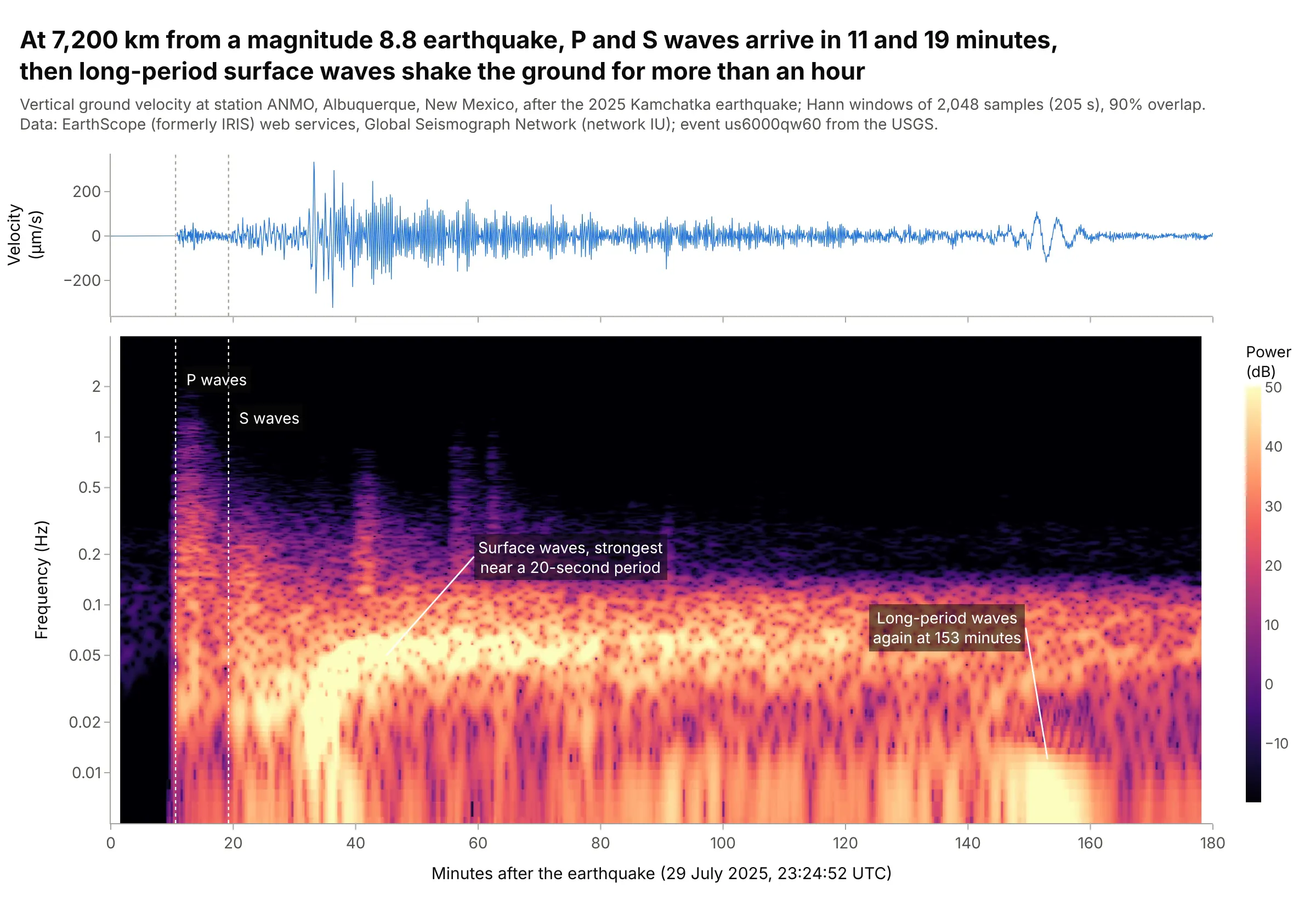
Spectrogram of three hours of vertical ground velocity at Albuquerque after the 2025 Kamchatka earthquake, with the seismogram above, log frequency axis from 0.005 to 4 Hz: P waves arrive at 10.6 minutes with power up to 1 Hz, S waves at 19.2 minutes, surface waves strongest near 0.05 Hz from about 30 minutes onward, and a long-period packet near 0.01 Hz at 153 minutes

The P waves from the July 29, 2025 Kamchatka earthquake reached Albuquerque in 11 minutes and the S waves in 19, but the ground moved most, up to 334 micrometers per second, when the surface waves arrived at 33 minutes, strongest at periods near 20 seconds. The packet at 153 minutes is most likely surface waves that went the long way around the Earth. Data: EarthScope (formerly IRIS) web services, station IU.ANMO, Global Seismograph Network; event us6000qw60 from the USGS.

Tip: mark the predicted arrival times from an Earth model (ObsPy's TauP does it in one line of code) as dotted lines through both panels.

Get the data from the EarthScope FDSN dataselect web service (network IU, station ANMO, location 00, channel
BHZ, 2025-07-29 23:20 to 2025-07-30 02:30 UTC) with ObsPy, convert counts to velocity with the station's
sensitivity, and decimate to 10 samples per second (columns: t_s, vel_um_s).

Make a plotly spectrogram with 2,048-sample windows, a log frequency axis from 0.005 to 4 Hz, the seismogram
above on a shared x axis in minutes, and dotted lines at the P and S arrival times from obspy.taup (iasp91).

3. A night of sleep EEG

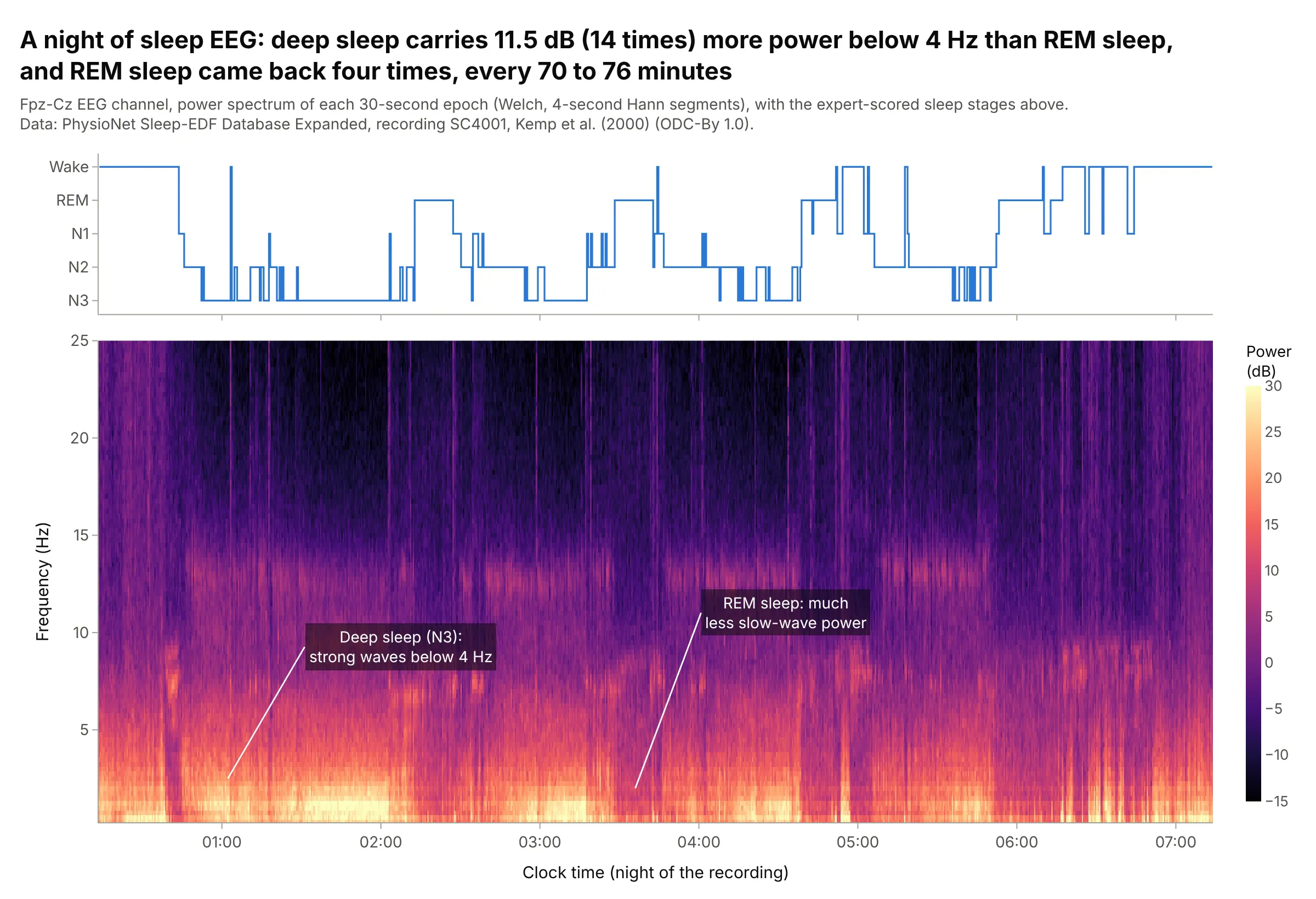
Whole-night spectrogram of the Fpz-Cz electroencephalography channel from 00:13 to 07:13 with the expert-scored hypnogram above: deep sleep (N3) periods are bright below 4 Hz, REM periods starting at 02:12, 03:28, 04:38 and 05:53 are darker below 4 Hz, and a faint band near 12 to 14 Hz appears during N2 sleep

In sleep medicine, a whole-night spectrogram of the electroencephalography (EEG), the brain's electrical activity measured on the scalp, shows the night's structure at a glance. In this recording, deep sleep (stage N3) carried 11.5 dB, 14 times, more power below 4 Hz than rapid eye movement (REM) sleep, and REM sleep came back four times, every 70 to 76 minutes. Data: PhysioNet Sleep-EDF Database Expanded, recording SC4001, Kemp et al. (2000) (ODC-By 1.0).

Tip: put the hypnogram (the sleep stages over time) above as a step line on the same clock-time axis, so each band of color lines up with its stage.

Get the data from PhysioNet's Sleep-EDF Database Expanded (sleep-cassette/SC4001E0-PSG.edf, channel EEG Fpz-Cz
at 100 Hz, and SC4001EC-Hypnogram.edf with the expert stages) and compute a Welch spectrum for every 30-second
epoch from 0.25 to 25 Hz (columns: time, stage, then one column per frequency in dB).

Make a plotly spectrogram from 0 to 25 Hz on a linear axis, the hypnogram above as a step line (Wake, REM, N1,
N2, N3) on a shared clock-time axis, and dB clipped from -15 to 30.

4. A ball bearing with an inner-race fault

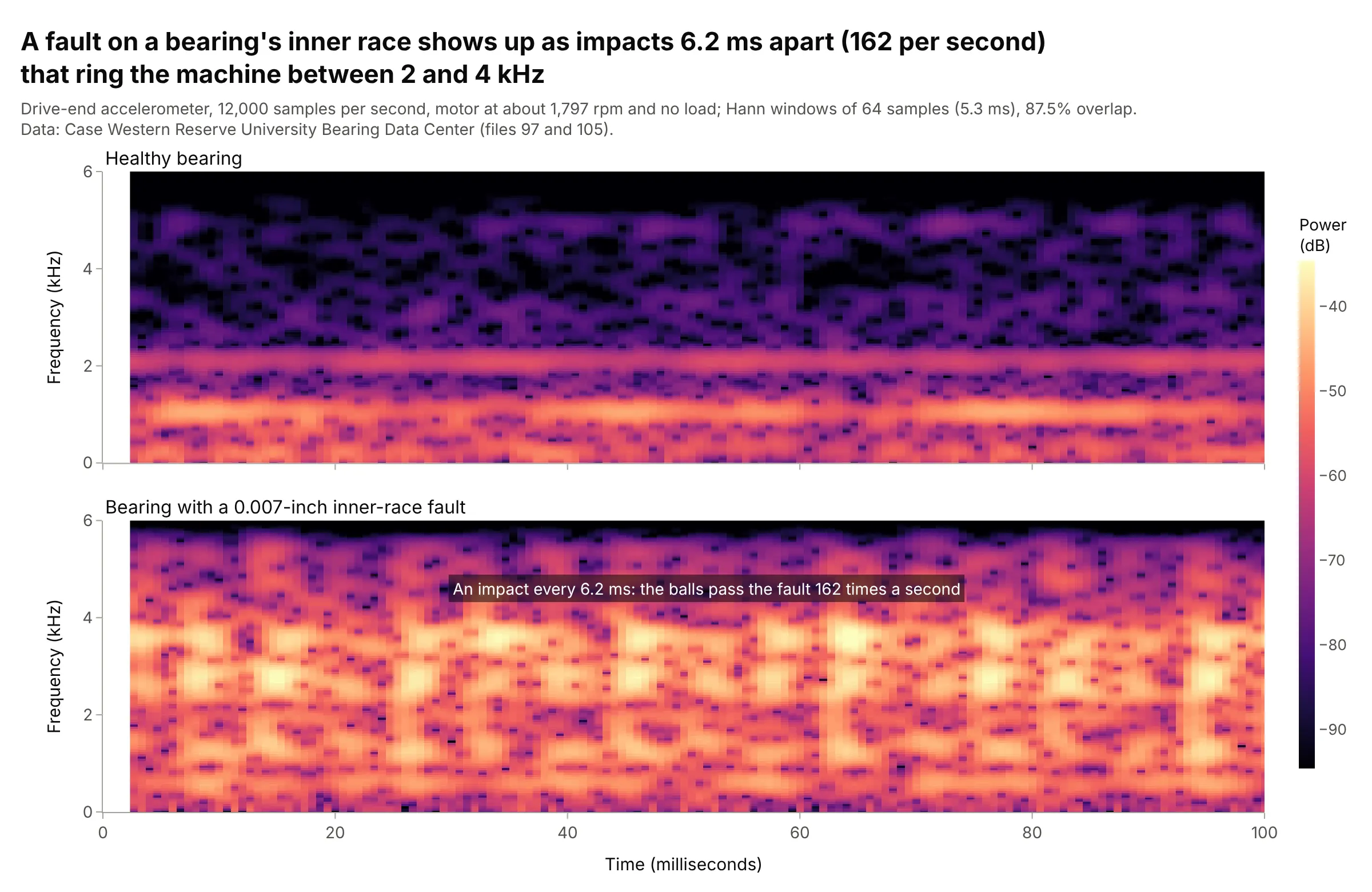
Two spectrograms of one-tenth of a second of bearing vibration from 0 to 6 kHz with 5.3 ms windows: the healthy bearing shows steady horizontal bands near 1 and 2.2 kHz; the bearing with a 0.007-inch inner-race fault shows bright vertical stripes between 2 and 4 kHz, about 6.2 ms apart

Each time a ball rolls over a 0.007-inch pit in the inner race it strikes it, and the impacts ring the machine between 2 and 4 kHz. With 5.3 ms windows they show as vertical stripes 6.2 ms apart, 162 per second, which is the bearing's inner-race defect frequency at 1,797 rpm, and the 2 to 4 kHz band is 21 times (26 dB) stronger than in the healthy bearing. Data: Case Western Reserve University Bearing Data Center, files 97 and 105.

Tip: for impacts, use a window shorter than the gap between them, so each one gets its own column.

Get the data from the Case Western Reserve University Bearing Data Center (12k drive end bearing fault data:
97.mat, normal, and 105.mat, inner race fault 0.007 inch, both at 0 hp and about 1,797 rpm, drive-end
accelerometer at 12,000 samples per second) (columns: t_s, normal_g, inner_race_fault_g).

Make two plotly spectrograms stacked with shared axes and one color scale, 64-sample Hann windows, 0 to 6 kHz,
the first 100 ms in milliseconds.

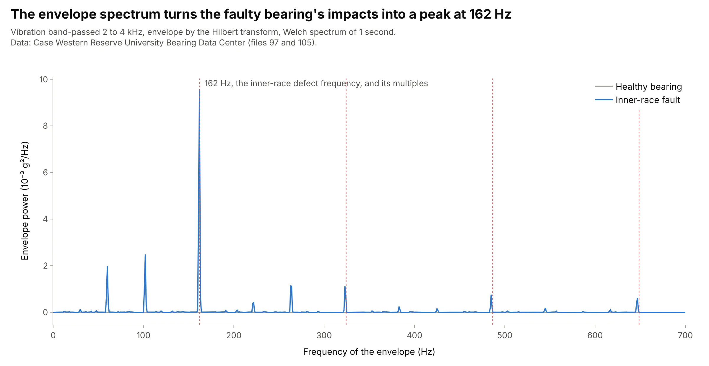
Another way to see it: vibration analysts turn the impacts into one number with an envelope spectrum: band-pass the signal around the resonance, take its envelope, and compute the envelope's spectrum, which peaks at the defect frequency.

Envelope spectrum of the faulty bearing from 0 to 700 Hz: a tall peak at 162 Hz, the inner-race defect frequency, and smaller peaks at its multiples near 324, 487 and 649 Hz, each marked with a dotted red line; the healthy bearing's envelope spectrum is flat near zero

5. A solo trumpet phrase, with a musical frequency axis

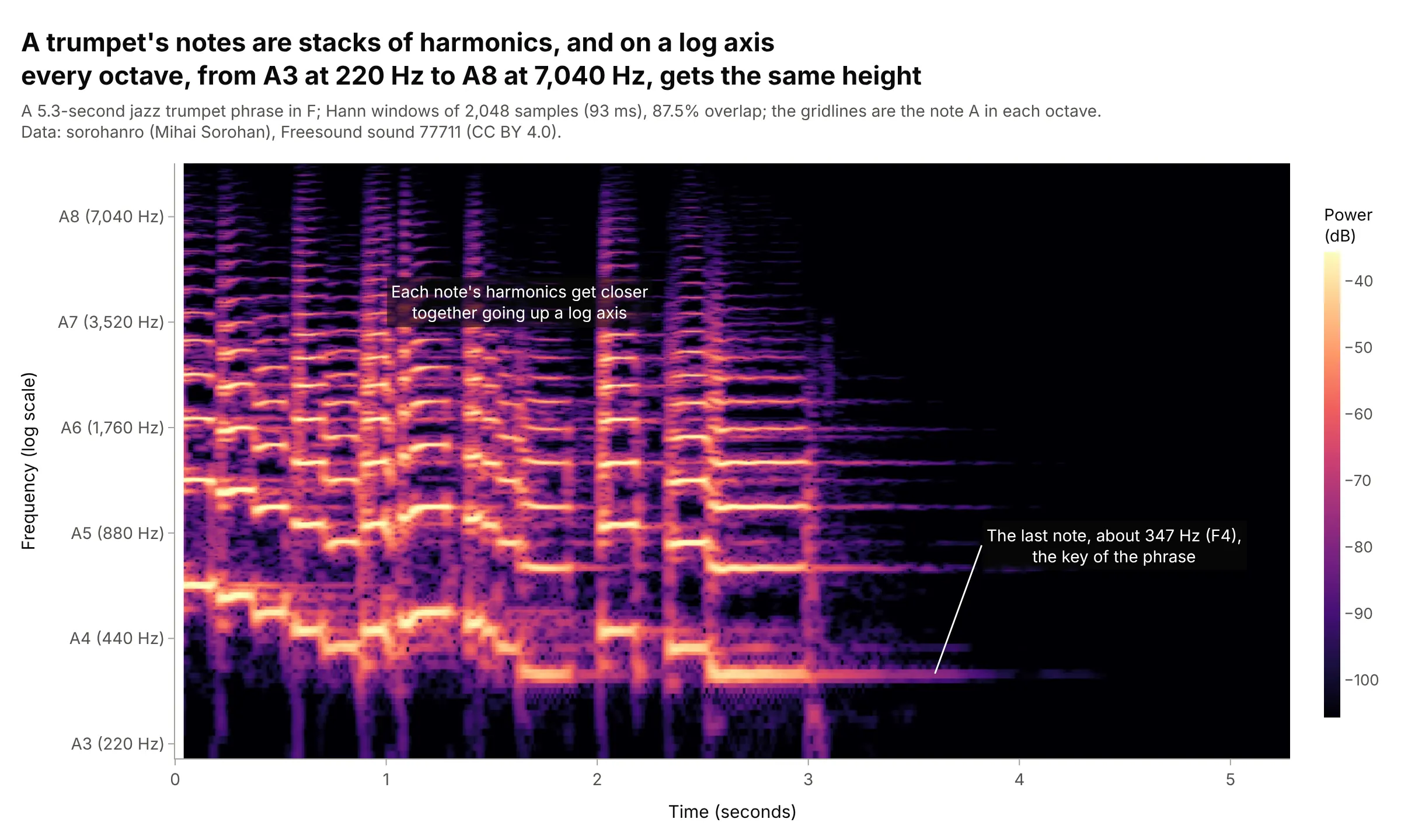
Spectrogram of a 5.3-second jazz trumpet phrase on a log frequency axis from 200 Hz to 10 kHz with gridlines at the note A in each octave from A3 (220 Hz) to A8 (7,040 Hz): each note is a stack of harmonics that get closer together going up, and the last note near 347 Hz (F4) rings on after 3 seconds

On a log frequency axis every octave gets the same height, like a piano keyboard, so a melody moves up and down as a pattern of stacked harmonics, and gridlines at each A from 220 Hz to 7,040 Hz turn the axis into a musical one. The phrase ends on a note near 347 Hz, F4, the key of the loop. Data: sorohanro (Mihai Sorohan), Freesound sound 77711 (CC BY 4.0).

Tip: for music, use windows of about 50 to 200 ms so neighboring notes, a few percent apart in frequency, separate.

Get the data from Freesound sound 77711 ("solo trumpet -06in F - 90bpm.wav" by sorohanro, CC BY 4.0), mixed to
mono and resampled to 22,050 Hz (columns: time_s, amplitude).

Make a plotly spectrogram with 2,048-sample Hann windows, a log y axis from 200 Hz to 10 kHz with ticks and
gridlines at A3 to A8 (220 to 7,040 Hz), and dB clipped to the top 70 dB.

6. A boat engine's whine over humpback whale song

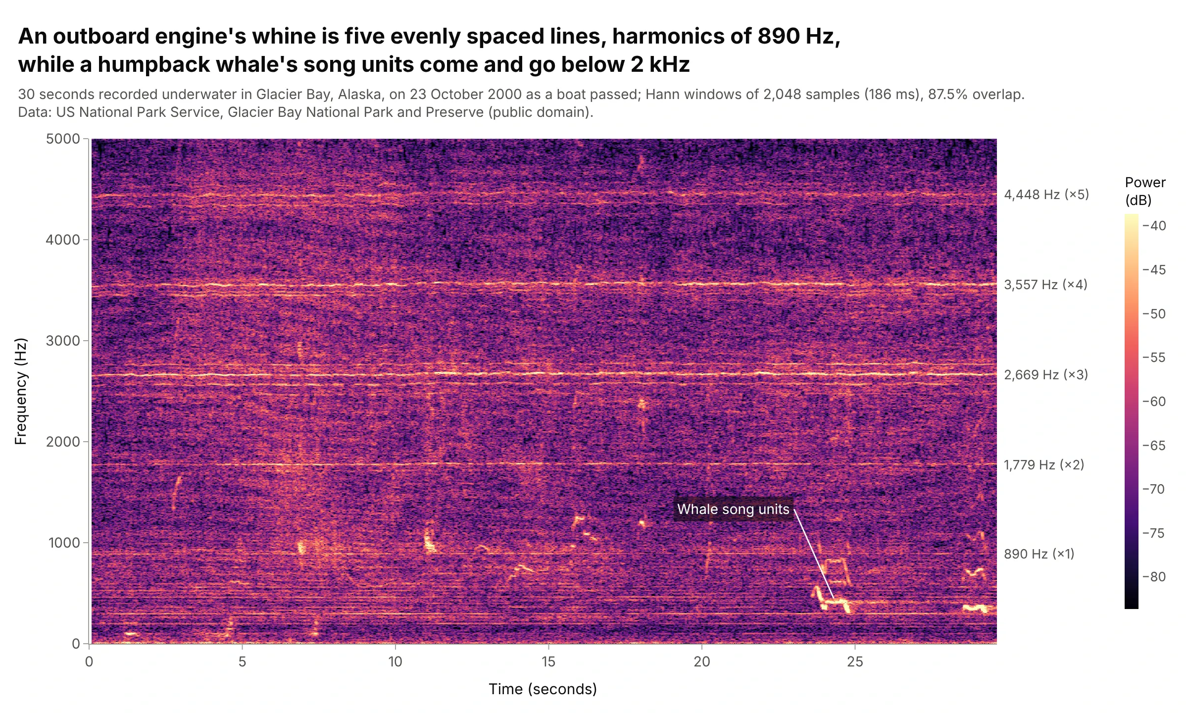
Spectrogram of 30 seconds of underwater sound in Glacier Bay on a linear axis from 0 to 5 kHz as a boat passes: five evenly spaced horizontal lines at 890, 1,779, 2,669, 3,557 and 4,448 Hz, labeled as 1 to 5 times 890 Hz, run across the whole recording, while short curved humpback whale song units come and go below 2 kHz

Ocean acousticians separate vessel noise from marine life by shape: this outboard engine's whine is five evenly spaced horizontal lines, the harmonics of 890 Hz, while the whale's song units are short curves below 2 kHz. A linear frequency axis keeps the harmonics evenly spaced, which makes them easy to recognize as one source. Data: US National Park Service, Glacier Bay National Park and Preserve (public domain), recorded 23 October 2000.

Tip: to find steady tones, take the median of every frequency row over time; lines stand out and short calls drop out.

Get the data from the US National Park Service's Glacier Bay sound clips page
(Humpback_whale_song_-_outboard_23Oct00-0909.mp3, "Outboard Engine Whine and Humpback Whale Song"), mixed to
mono and resampled to 11,025 Hz (columns: time_s, amplitude).

Make a plotly spectrogram with 2,048-sample Hann windows, a linear y axis from 0 to 5 kHz, and the engine's
harmonic frequencies labeled on the right edge.