Levey-Jennings Charts - A Complete Guide

TL;DR

• A Levey-Jennings chart plots a laboratory's results for a control material, a sample whose concentration is known and never changes, in run order, with a line at the mean and lines at 1, 2 and 3 standard deviations (SD) either side, so the lab can tell whether a test is working before it reports any patient results.
• Levey-Jennings charts are also known as Levey-Jennings control charts, and are similar to control charts (Shewhart's individuals chart) and line charts. Clinical laboratories read them with the Westgard rules: 1-2s is a warning, and 1-3s, 2-2s, R-4s, 4-1s and 10-x reject the run.
• US clinical laboratories run at least two control materials of different concentrations every day they test patients, and each gets its own Levey-Jennings chart (or a shared one in SD units).
• You can make a Levey-Jennings chart with Plotly from a go.Scatter trace, seven horizontal lines and a second trace for the results that break a rule, and a short helper function is below.

What is a Levey-Jennings chart?

Every laboratory test drifts a little: reagents age, lamps dim, a new lot of calibrator arrives, a pipette starts to stick. A laboratory can't see that drift in patient samples, because every patient's value is different. So alongside the patients it measures a control material, a stable sample (often pooled serum, or for water labs, water of known composition) whose true value doesn't change from day to day. Any movement in the control's results is the measurement moving, and the Levey-Jennings chart is where the lab watches for it.

Levey-Jennings charts look like this:

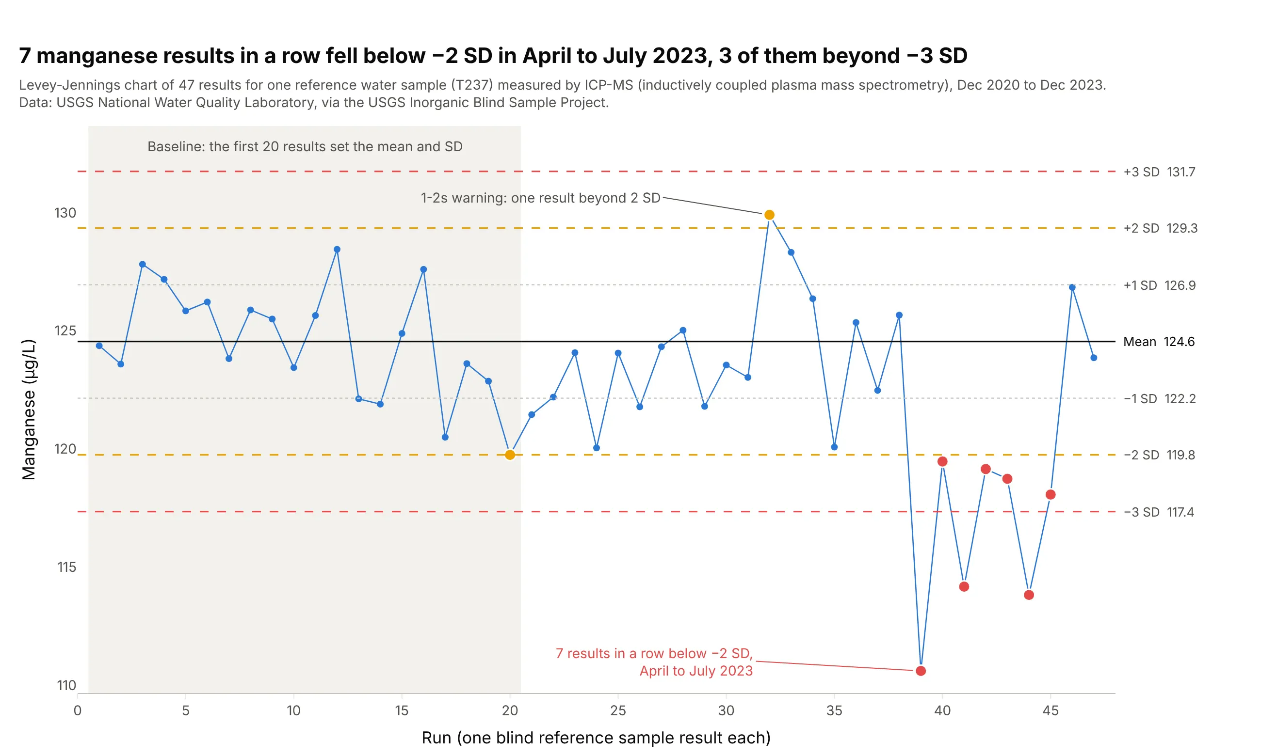
Data: USGS (US Geological Survey) National Water Quality Laboratory, via the USGS Inorganic Blind Sample Project.

How do you read a Levey-Jennings chart? In the example above, notice these things:

• Each point is one result for the same reference water sample, measured by ICP-MS (inductively coupled plasma mass spectrometry), in the order the lab ran them. The sample never changes, so the points should scatter around one value.
• The black line is the mean of the first 20 results, 124.6 µg/L, and the dotted, amber and red lines sit at 1, 2 and 3 SD from it (the SD of those 20 results is 2.40 µg/L). In a stable test about 68% of results land within 1 SD and 95% within 2 SD.
• Two amber results (runs 20 and 32) are just beyond 2 SD. That is a 1-2s warning: about 1 result in 22 lands there by chance, so the lab looks closer but doesn't reject the run.
• From April to July 2023, seven results in a row sat below −2 SD and three of them below −3 SD, which breaks the 1-3s and 2-2s rules. Something changed in the method for manganese, and in December 2023 the results were back near the mean.

It's often used for charts like these:

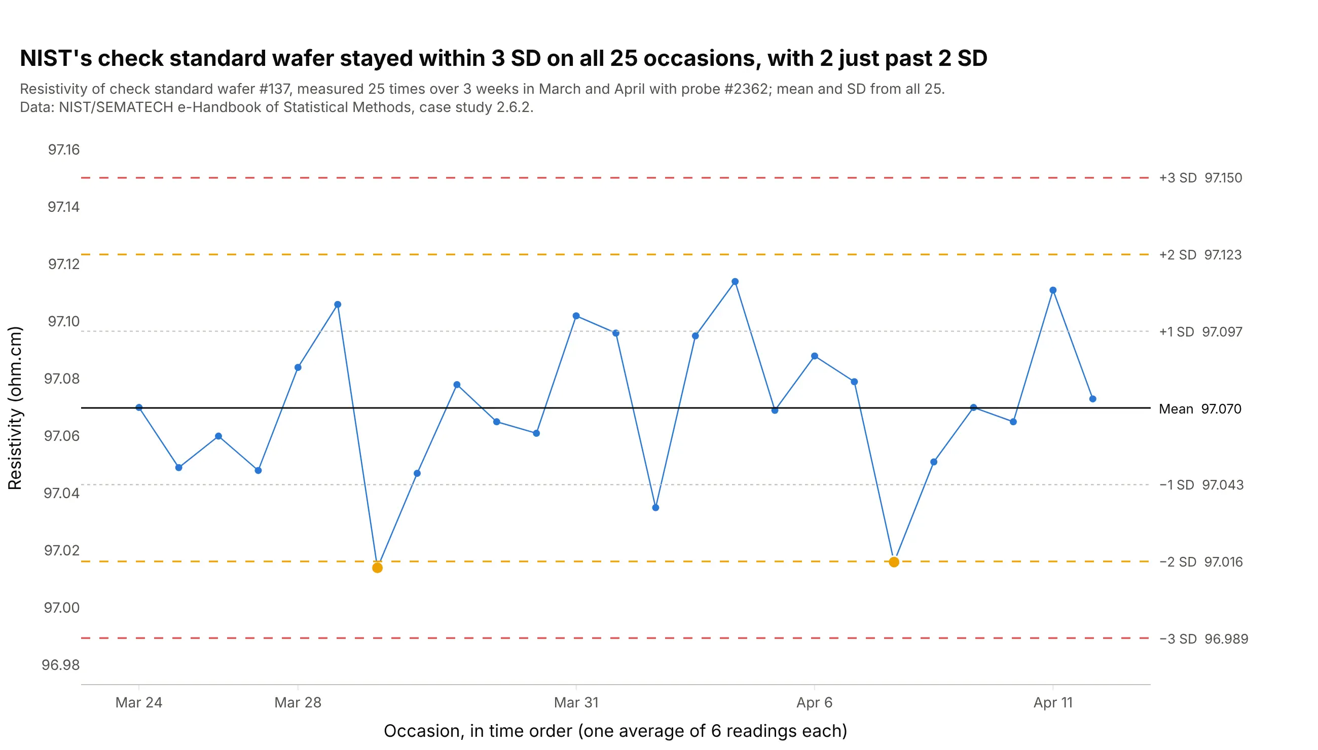
Check standards in measurement laboratories. NIST (the US National Institute of Standards and Technology) measured one silicon wafer 25 times while it certified others from the same crystal, and all 25 values stayed within 3 SD of the mean of 97.070 ohm.cm. Data: NIST/SEMATECH e-Handbook of Statistical Methods, 2.6.2.

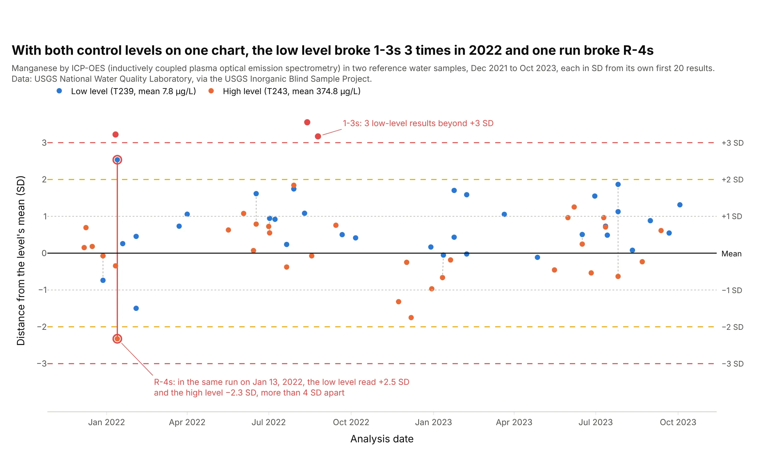
Daily quality control with two control levels. US rules for clinical labs (in the Code of Federal Regulations, 42 CFR 493.1256) ask for two control materials of different concentrations each day they test patients, so labs draw both on one chart in SD units; here a low and a high manganese sample broke the R-4s rule in the same run on January 13, 2022. Data: USGS National Water Quality Laboratory, Inorganic Blind Sample Project.

Hospital and commercial clinical laboratories keep their daily quality control (QC) results private, and no public clinical series turned up in a search of open data repositories and journal supplements, so the examples in this guide use the public QC record of the USGS National Water Quality Laboratory (NWQL) in Denver. The USGS sends it blind reference samples, water of known composition disguised as ordinary samples, and publishes every result, with charts back to 1985. Several of the analytes (sodium, potassium, calcium, iron) are ones a hospital chemistry analyzer measures in blood too, and the chart and the rules work the same way.

A short history

Walter Shewhart invented the control chart for manufacturing at Bell Labs in the 1920s (Shewhart 1926). In 1950 two pathologists, Stanley Levey and E. R. Jennings, proposed using it in the clinical laboratory (Levey and Jennings 1950); they measured patient specimens in duplicate and charted the range between the two. Two years later Richard Henry and Milton Segalove recommended a pooled patient sample as a stable control and plotting each single measurement of it (Henry and Segalove 1952), which is the chart labs still call a Levey-Jennings chart (Westgard, "QC Past, Present and Future"). In 1981 James Westgard and colleagues published the multirule procedure that labs use to read it today (Westgard et al. 1981).

What is a control material?

A control material is a sample that behaves like a patient specimen but is made to be the same every time. For blood tests, a laboratory usually buys it from a manufacturer, who makes one large batch (a lot) of pooled serum or a similar fluid, in liquid or freeze-dried vials. A good control material has the same kind of matrix as patient samples (the same fluid and background chemistry), stays stable for a long time, and comes in a batch big enough to last at least a year (Wikipedia, "Laboratory quality control"). The lab measures it alongside patients: usually at the start of each shift, after the instrument is serviced, when a new reagent lot is loaded, and after calibration (same source).

A control is not a calibrator. A calibrator is used to set the instrument's scale, and a control is measured afterward to check that the scale still holds. Controls also come at more than one concentration, called levels, such as a normal and an abnormal value, because a test can work in the middle of its range and fail at the ends.

The mean printed on a control's insert comes from many laboratories, so each lab measures its own control on at least 10 days and uses its own mean and SD, as in the next section.

How the lines are set

A Levey-Jennings chart has seven horizontal lines, and all of them come from two numbers: the mean and the SD of the control's results while the test is known to be working.

The lab first measures a new control material on many separate days, at least 20 measurements over at least 10 days in the Westgard QC lesson on the chart. The mean of those results is the center line. The SD measures how far a typical result sits from the mean, and the lines go at the mean plus and minus 1, 2 and 3 SD. If the results follow a normal (bell-shaped) distribution, 68.3% of them fall within 1 SD, 95.4% within 2 SD and 99.7% within 3 SD:

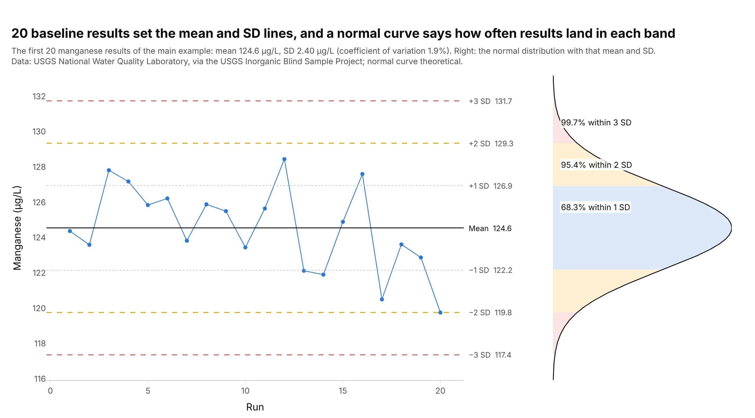
Data: the first 20 results of the manganese chart above; normal curve theoretical.

Labs often quote the SD as a share of the mean, the coefficient of variation (CV). For these 20 manganese results the SD is 2.40 µg/L on a mean of 124.6, a CV of 1.9%.

Those percentages are why the rules are set where they are. A result beyond 2 SD happens 4.6% of the time by chance, so with two control levels a run would be rejected for nothing about 9% of the time; that's why 1-2s is only a warning. A result beyond 3 SD happens 0.27% of the time, so 1-3s rejects a run with few false alarms.

The lines stay fixed once they are set. The lab recalculates them when it starts a new lot of control material, which comes with a slightly different concentration, and not every time a result looks odd.

The Westgard rules

The Westgard multirule procedure reads the chart with six rules (Westgard Rules). The first is a warning and the other five reject the run, which means the lab holds the patient results from that run, finds the problem and reruns them:

1. 1-2s (warning): one result beyond 2 SD. Check the other rules before accepting the run.
2. 1-3s: one result beyond 3 SD. Usually a random error, such as a bubble or a pipetting slip.
3. 2-2s: two results in a row beyond the same 2 SD line, either the same control in consecutive runs or two control levels in one run. A systematic error, such as a calibration shift.
4. R-4s: in one run, one control beyond +2 SD and another beyond −2 SD, more than 4 SD apart. Random error; Westgard says to apply it only within a run.
5. 4-1s: four results in a row beyond the same 1 SD line. A small systematic shift.
6. 10-x: ten results in a row on the same side of the mean. A small shift or a slow drift.

In the names, the first number is how many results are involved, the second is how far from the mean they sit, and the "s" stands for SD, so 2-2s means two results beyond 2 SD. R-4s is a range of more than 4 SD, and 10-x means ten results on one side of the mean (x is the mean).

Here is each rule where it fired in the USGS control results:

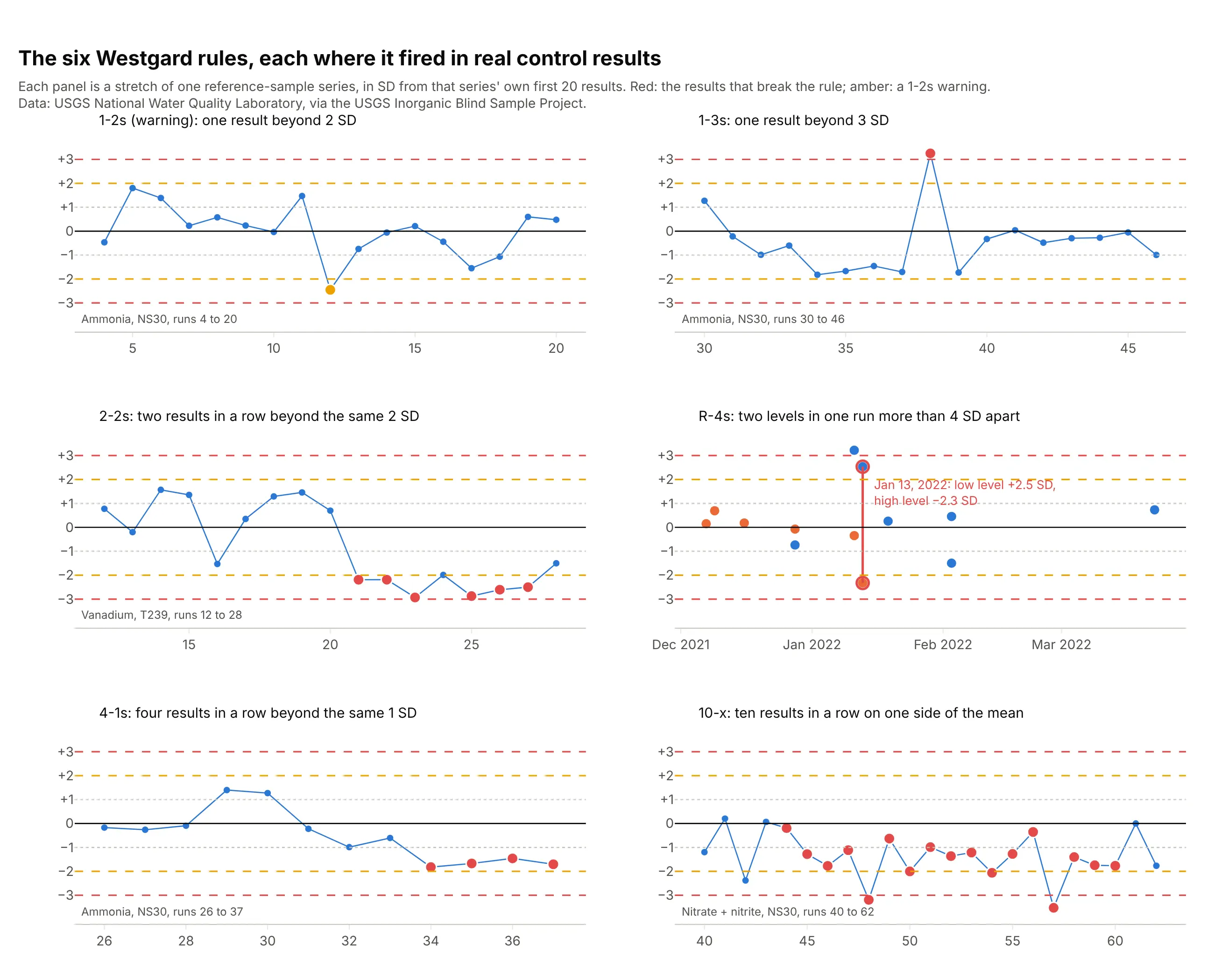
Data: USGS National Water Quality Laboratory, Inorganic Blind Sample Project; rules from Westgard et al. 1981.

Which rule fired also says what kind of error to look for. Rules that look at a single result (1-3s, R-4s) catch random errors, and rules that look at a run of results (2-2s, 4-1s, 10-x) catch systematic ones, which usually come from calibration, reagents or the instrument.

Levey-Jennings charts and control charts

A Levey-Jennings chart is a control chart, and its three conventions are what make it a laboratory chart. It plots a control material whose true value is fixed, not the product or the patients; it sets its lines from the plain SD of 20 or more baseline results, where Shewhart's individuals chart estimates sigma from the moving range, the jump between consecutive points; and it draws 1 and 2 SD lines and reads them with the Westgard rules, where a manufacturing chart usually draws only the 3-sigma limits and uses the Western Electric rules. On the manganese data the two ways of estimating the spread give 2.40 µg/L from the SD and 2.13 µg/L from the moving range, so the limits end up close.

Alternatives to a Levey-Jennings chart

Here's the same manganese data drawn six ways. Some are better for the question, some worse, some just different:

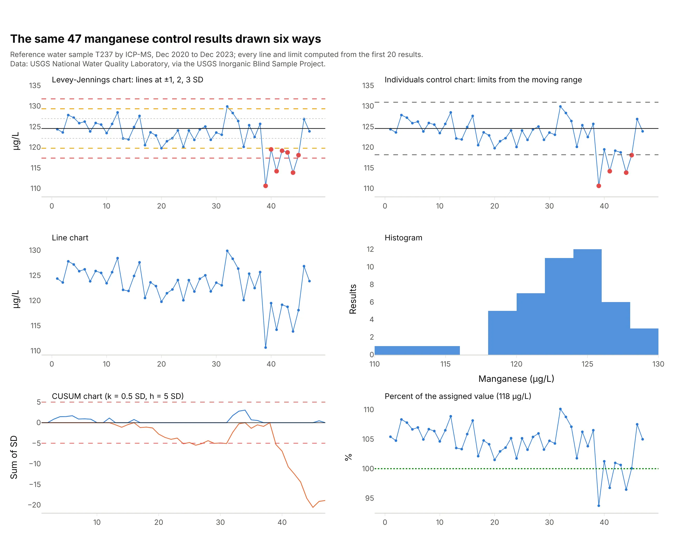
Data: USGS National Water Quality Laboratory, Inorganic Blind Sample Project.

• Individuals control chart (works too). Limits from the moving range land close to the 3 SD lines (118.2 and 130.9 µg/L) and flag 4 of the 7 low results, but without 1 and 2 SD lines it can't apply the 2-2s or 4-1s rules.
• Line chart (worse). The drop in 2023 is visible, but nothing says how far a result may wander by chance, so nobody can decide whether to reject a run.
• Histogram (different). It shows the spread and the low tail, which is useful when you set the lines, but it throws away the run order that the rules depend on.
• CUSUM (cumulative sum) chart (better for small shifts). Adding up each result's distance from the mean shows a small downward drift from run 24, well before the 2023 drop, but its scale, a sum of SDs, takes explaining at the bench.
• Percent of the assigned value (different). The USGS charts its blind samples against the value assigned to the material. That shows accuracy (this lab ran about 5.6% high until 2023) where the Levey-Jennings chart shows stability.

With many tests on one instrument, small multiples of Levey-Jennings charts in SD units show whether a problem hits one test or all of them (example 6 below).

How to make a Levey-Jennings chart

With AI

ChatGPT, Claude Code, GitHub Copilot, Cursor and other AI tools are excellent at writing Plotly code. Name Plotly in the prompt, and say which results set the lines and which rules to apply:

With Plotly Studio

Plotly Studio is a desktop app where you point an AI at a dataset and it builds charts and a Dash app around your questions. Ask for a Levey-Jennings chart the same way:

Show a Levey-Jennings chart of control results by run, with the mean and ±1, 2 and 3 SD lines from the first 20 runs, Westgard rule violations in red with the rule on hover, and dropdowns to pick the analyte and the control level.

Make a Levey-Jennings chart in Python or JavaScript

This is the code AI tools write under the hood. You can make a Levey-Jennings chart with Plotly from a go.Scatter of the control results, seven horizontal lines and a second trace for the results beyond 2 and 3 SD. This helper returns a go.Figure, and every chart in this guide builds on the same idea:

The width and opacity on each line matter with the simple_white template, which otherwise draws shapes with no line. For the rules, compute z as above and test each pattern in a loop over the runs, for example abs(z[i]) > 3 for 1-3s and z[i] > 2 and z[i - 1] > 2 (or both below −2) for 2-2s. For two control levels on one chart, plot z instead of the raw values, with the lines at −3 to 3.

In JavaScript, plotly.js draws the same thing with two scatter traces and seven line shapes:

Share it

Every Plotly chart has a Share chart button (the cloud icon in its toolbar) that uploads it to Plotly Cloud and gives you a link. Only you can see it until you change its visibility.

For a live app, put the chart in a Dash app and publish it with the Plotly Cloud CLI. Coding agents can run these commands for you:

If your data has to stay in your own cloud or data center, publish to Dash Enterprise instead.

Dos and don'ts

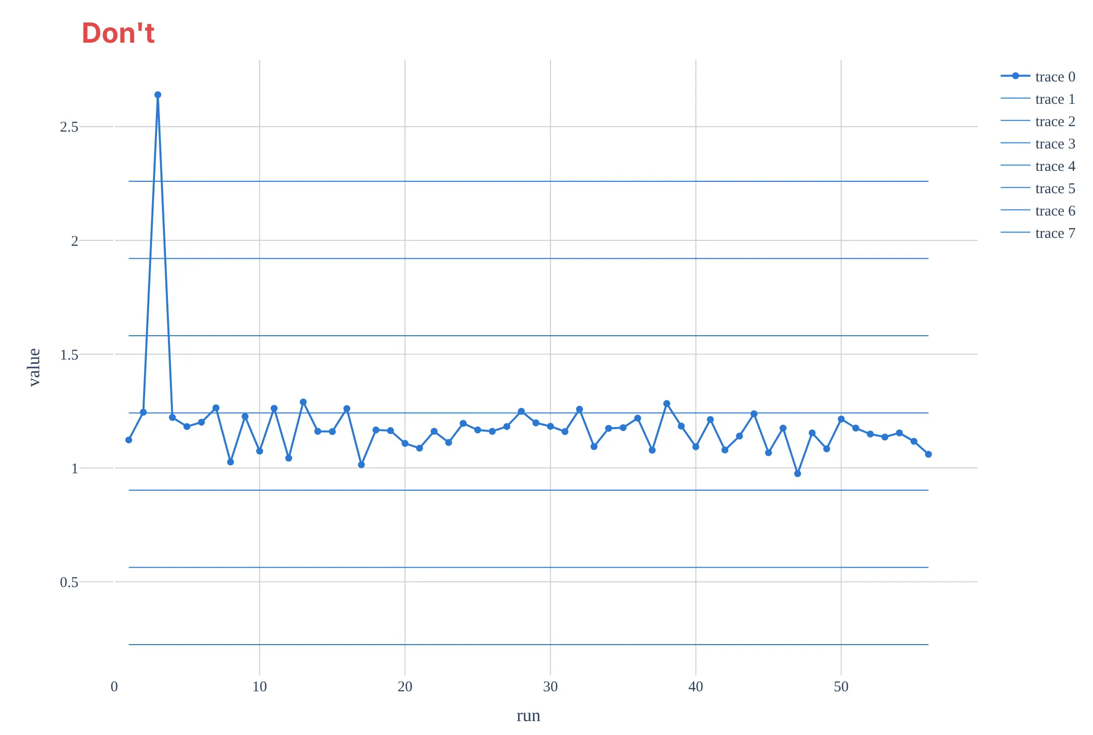
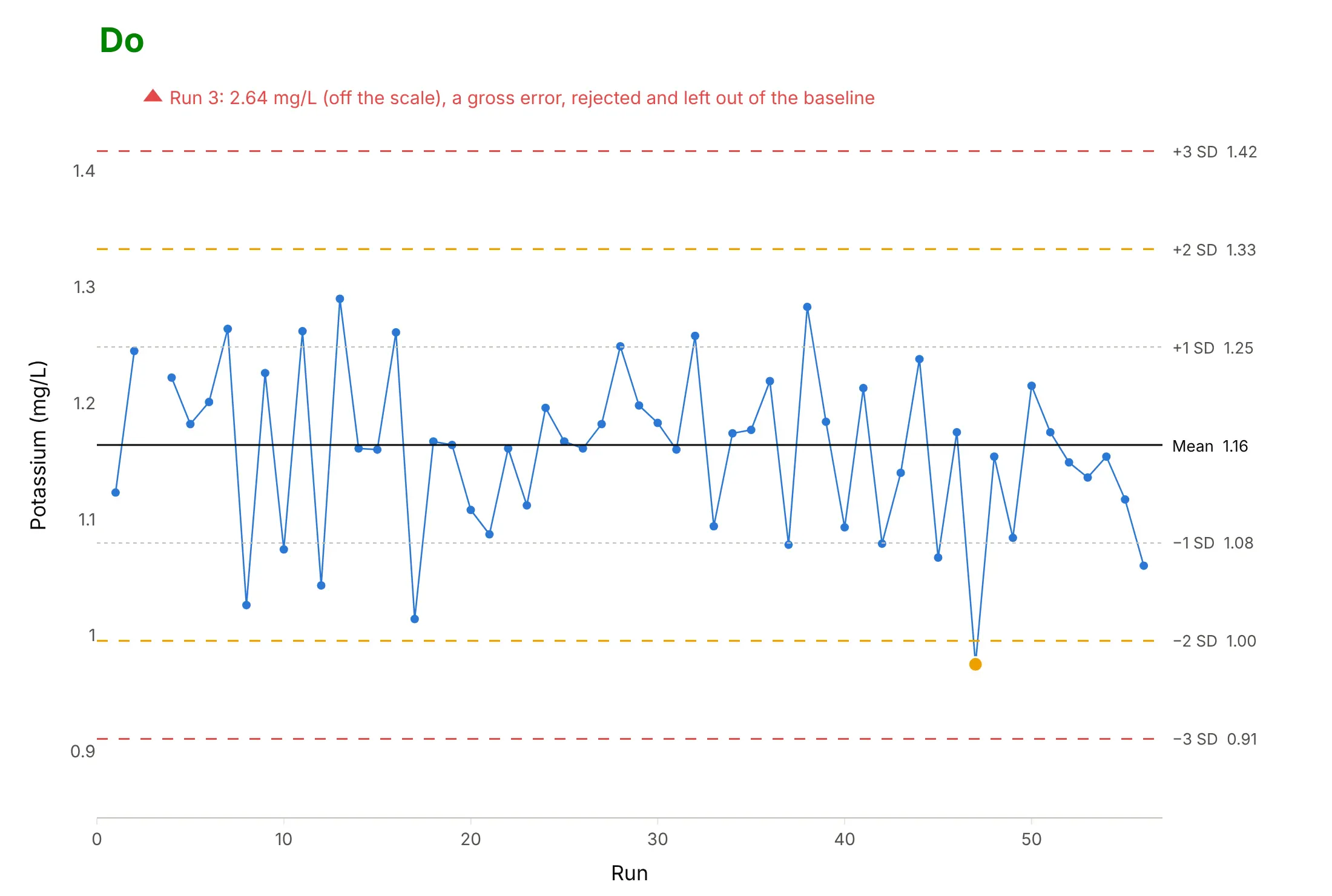
Most of the work in a Levey-Jennings chart is setting the mean and SD from clean baseline results and making the lines easy to tell apart. Here are 56 potassium results for one reference sample, in run order, both ways and in the same blue.

Don't compute the mean and SD from a baseline that includes a gross error (here run 3 read 2.64 mg/L, 2.3 times the sample's assigned value of 1.15, which makes the SD 0.339 mg/L instead of 0.084), draw every line in the data's color without labels, leave rule violations unmarked, or keep the default legend, raw column names and a serif font. With an SD four times too large, the lines are so far apart that no real problem could ever cross them:

Do reject the gross error and leave it out of the baseline, set the mean and SD from the other first 20 results (1.16 and 0.084 mg/L), draw the lines in their conventional styles with their values, and mark the one 1-2s warning:

Checklist

Do

• Set the mean and SD from at least 20 results on at least 10 different days, with obvious errors removed.
• Keep the lines fixed, and set new ones when a new lot of control material starts.
• Draw the mean solid, the 2 SD lines amber and the 3 SD lines red, labeled with their values.
• Run at least two control levels, and put them on one chart in SD units when you apply rules across levels.
• Mark every result that breaks a rule, and write down what you found and did.
• Check accuracy separately, against the material's assigned value or external proficiency testing.

Don't

• Use the manufacturer's range printed on the control's insert as your SD lines; it describes many laboratories, and your lines should describe yours.
• Recalculate the mean and SD every month from whatever results came in, which lets a slow drift move the lines with it.
• Reject runs on 1-2s alone.
• Draw a Levey-Jennings chart of patient results; patient values differ by person, so the lines mean nothing.

Options to customize

A Levey-Jennings chart in Plotly is a go.Scatter trace plus shapes, so these are the options that matter most. The full lists are in the scatter trace reference and the horizontal and vertical lines documentation.

1. go.Scatter(mode="lines+markers"): the control results in run order; use mode="markers" for several levels on one chart in SD units.
2. fig.add_hline(y=..., line_dash=..., line_color=...): the mean and the 1, 2 and 3 SD lines; set line_width and opacity when a template hides shapes.
3. annotation_text on add_hline, or add_annotation(xref="x domain", x=1): the line values at the right edge.
4. A second scatter trace with marker.color and marker.size: the results that break a rule, drawn on top.
5. hovertext and hovertemplate: the run, date, lot and the rule that fired on hover.
6. fig.add_vrect: shade the baseline runs, a reagent lot or a period of interest.
7. make_subplots(rows=..., cols=..., shared_yaxes=True): one panel per analyte or level, in SD units, as in the grid example.
8. xaxis.tickvals, xaxis.ticktext: dates as ticks when the x axis is the run number.
9. yaxis.range: fix the range at about ±4 SD so every chart in a binder or app reads the same way.

More Levey-Jennings chart examples

Seven more Levey-Jennings charts built from the USGS laboratory's public QC record, each with the rule or technique it shows and a prompt to rebuild it.

1. Vanadium: a shift of 2 SD that stayed for 20 runs

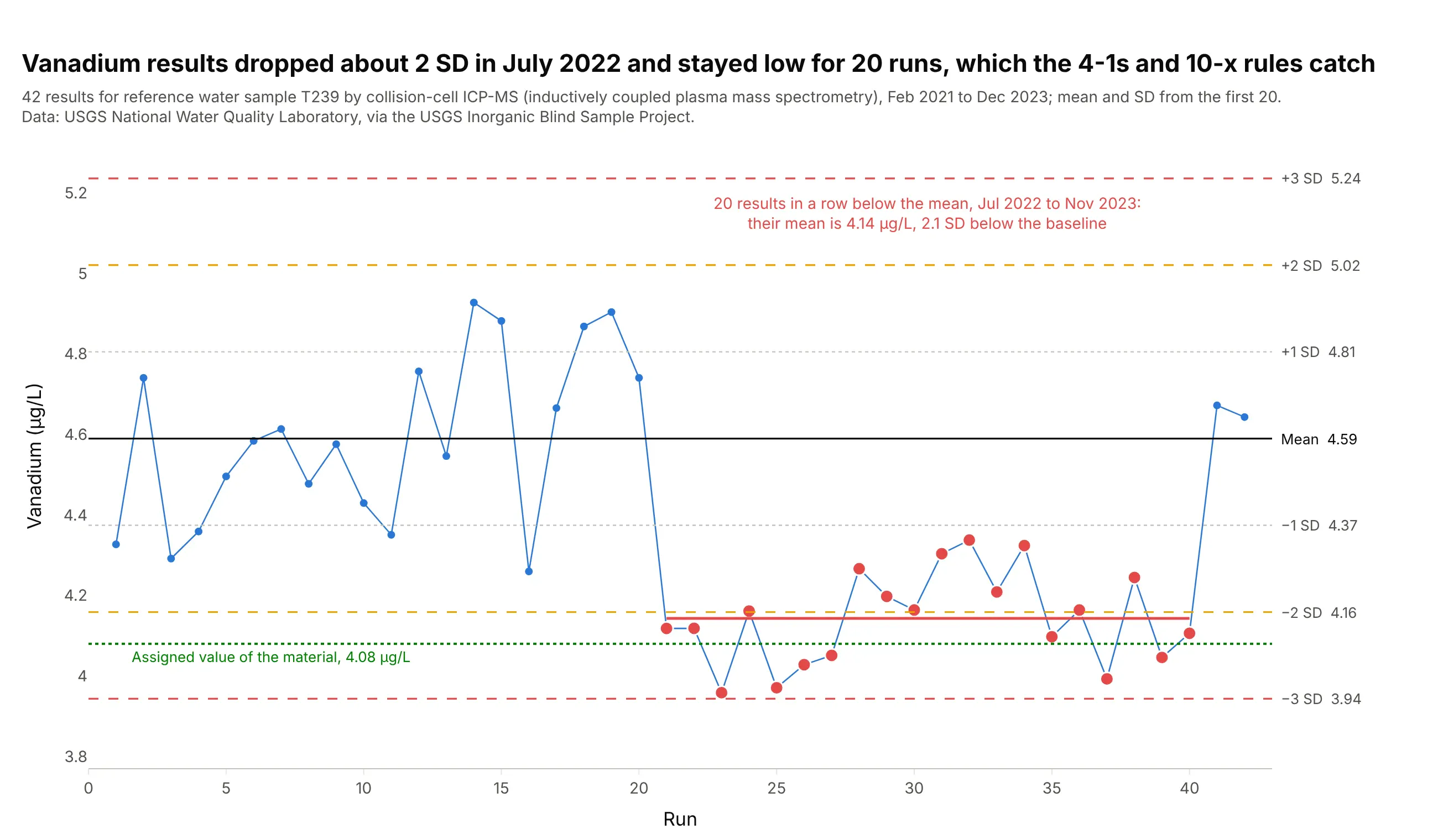
From July 2022 to November 2023, all 20 vanadium results sat below the mean, averaging 4.14 µg/L against a baseline of 4.59, a shift of 2.1 SD that the 2-2s, 4-1s and 10-x rules all catch. The shift moved the results toward the material's assigned value of 4.08 µg/L, which is a reminder that the chart detects change, not error. Data: USGS National Water Quality Laboratory, Inorganic Blind Sample Project.

Tip: draw the shifted period's own mean as a short segment, so readers see the size of the shift in the chart's units.

2. Nitrate: 17 results in a row below the mean

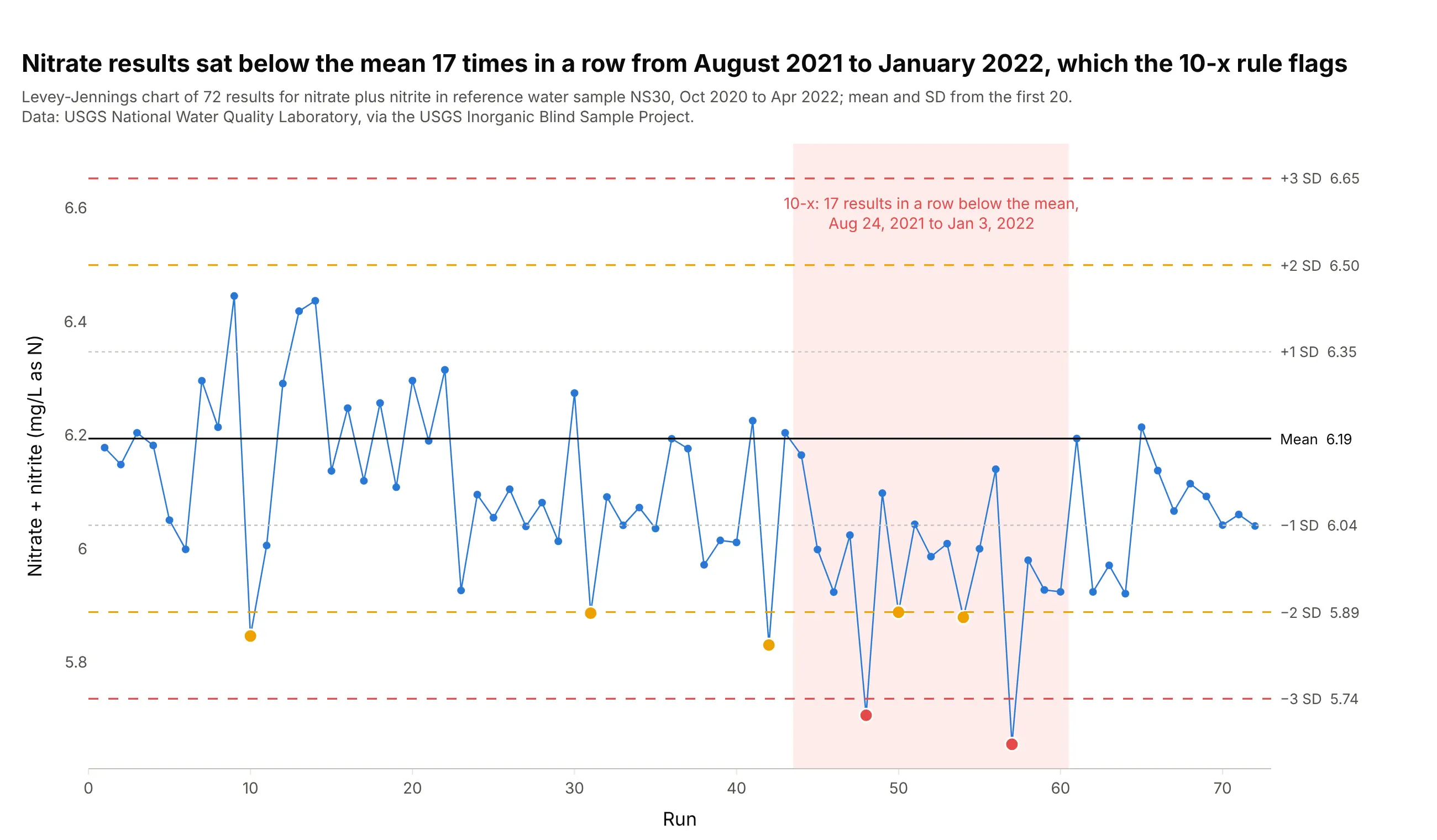
From August 24, 2021 to January 3, 2022, 17 nitrate results in a row came in below the mean of 6.19 mg/L as nitrogen. Ten in a row on one side happens by chance about once in 512 tries, so the 10-x rule flags a persistent small bias. Here it also showed up as two results beyond 3 SD, but 13 of the 17 results were within 2 SD, so no single point would alarm anyone, which is the case 10-x exists for. Data: USGS National Water Quality Laboratory, Inorganic Blind Sample Project.

Tip: shade the run that breaks 10-x, because a run of ordinary-looking points is easy to overlook.

3. Ammonia: one result beyond +3 SD

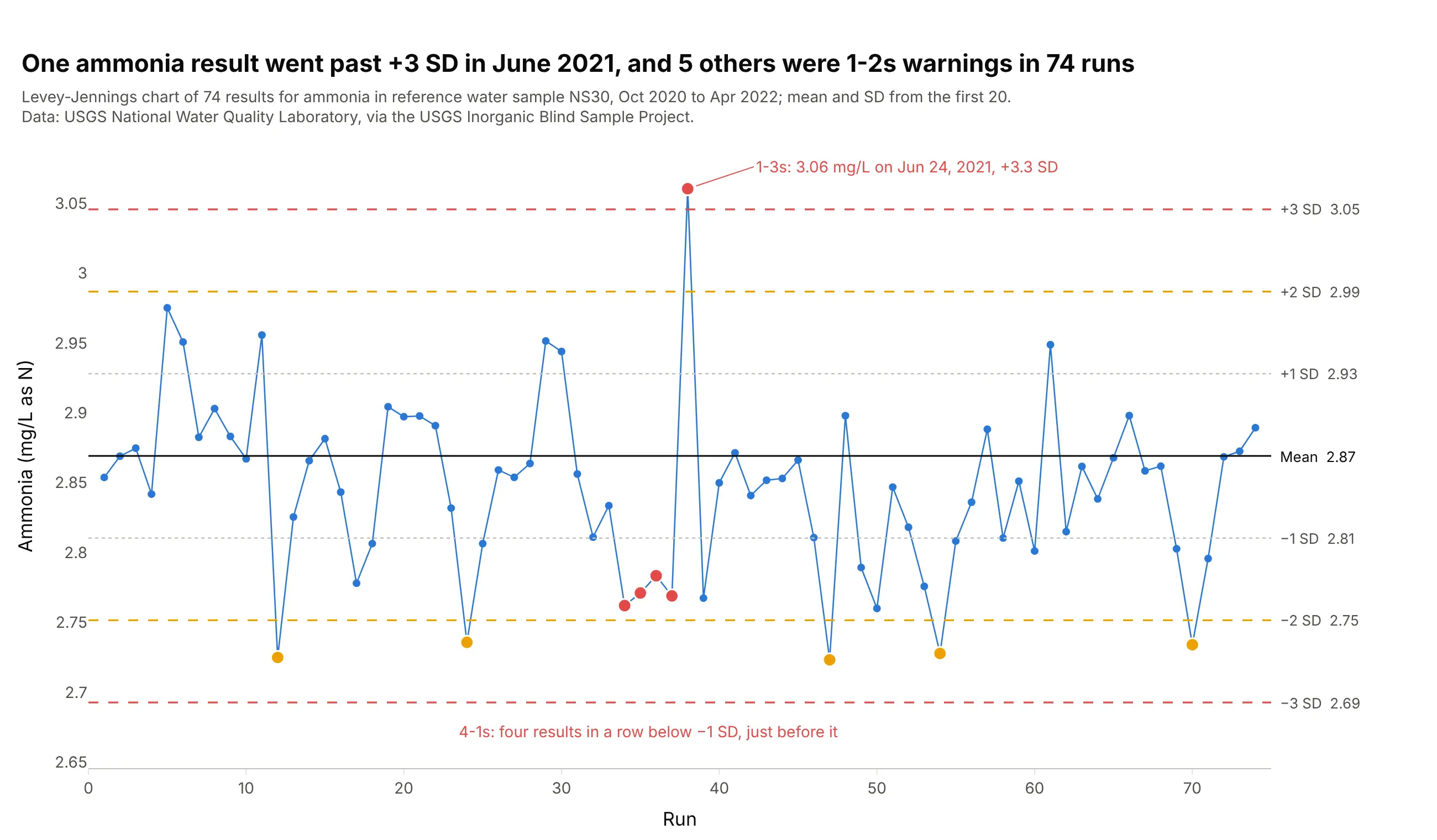
One ammonia result, 3.06 mg/L on June 24, 2021, landed 3.3 SD above the mean, with ordinary results on both sides of it, the signature of a random error in that one run. With five other 1-2s warnings, 6 of 74 results fell beyond 2 SD, against about 3 expected by chance. Data: USGS National Water Quality Laboratory, Inorganic Blind Sample Project.

Tip: label a 1-3s result with its value and date, because that's what the person investigating it will search for.

4. Boron: in control, and 18% high

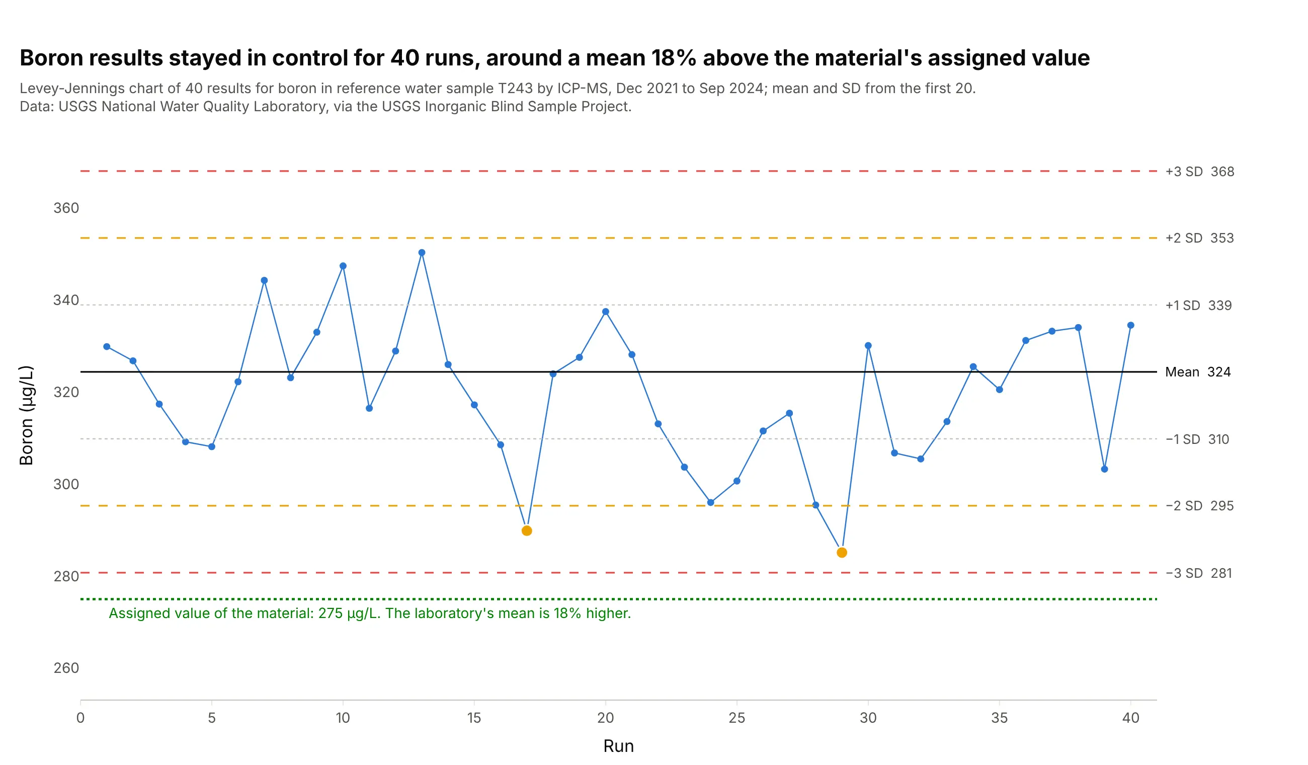
All 40 boron results stayed inside 3 SD of their mean of 324 µg/L, with two 1-2s warnings, so by the Westgard rules the method was stable throughout. Its mean is 18% above the 275 µg/L assigned to the material, a bias the chart can't see because its lines come from the lab's own results. Data: USGS National Water Quality Laboratory, Inorganic Blind Sample Project.

Tip: add the assigned or target value as its own line in a different color, so stability and accuracy are both on one chart.

5. Sodium: what a stable test looks like

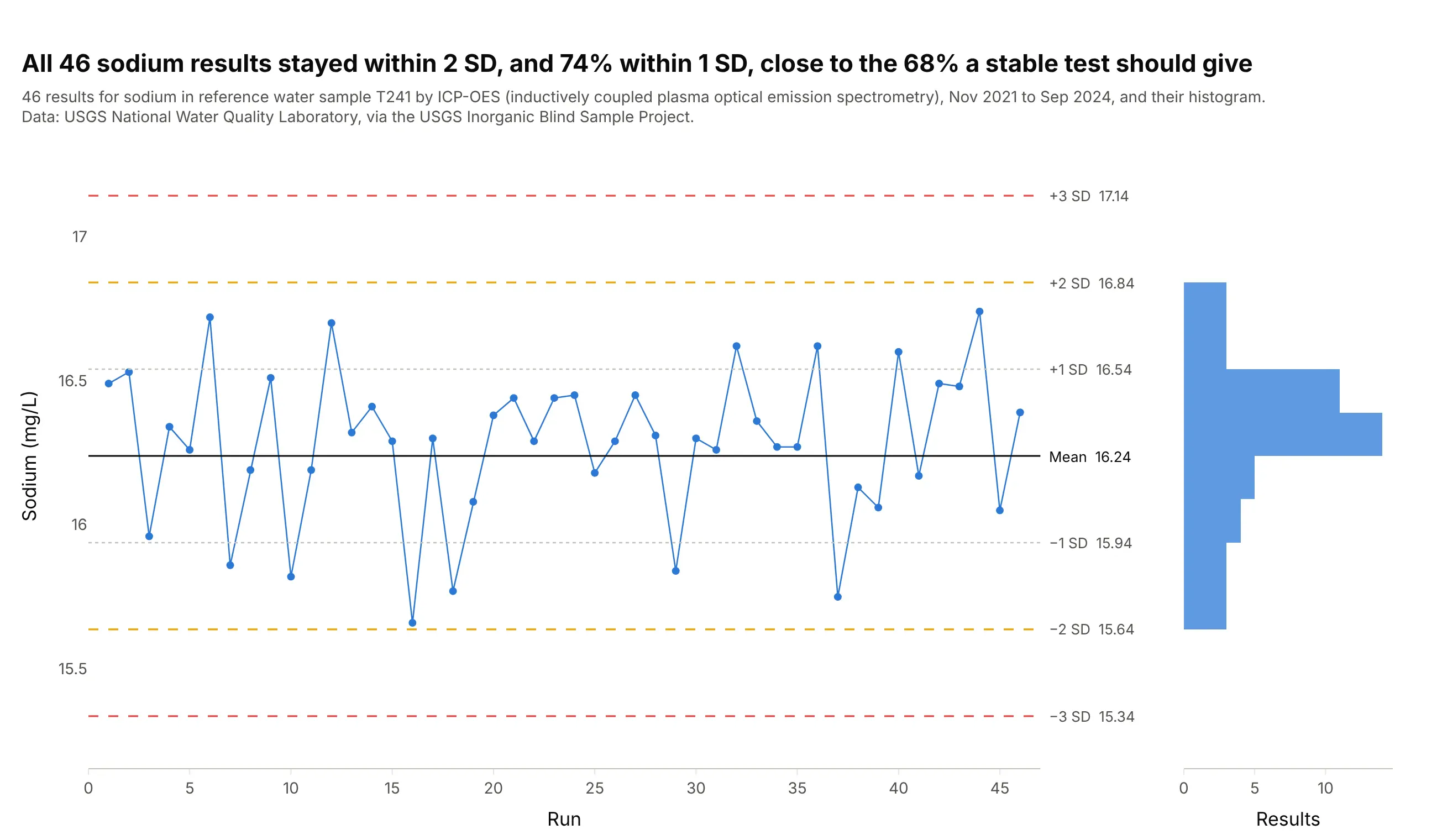
All 46 sodium results stayed within 2 SD of the mean, 74% of them within 1 SD, close to the 68% a normal distribution predicts, and no rule fired from November 2021 to September 2024. A histogram on its side next to the chart shows the bell shape the lines assume. Data: USGS National Water Quality Laboratory, Inorganic Blind Sample Project.

Tip: share the y axis between the chart and the histogram so each bar lines up with its band.

6. Nineteen elements on one instrument: was it manganese or the whole run?

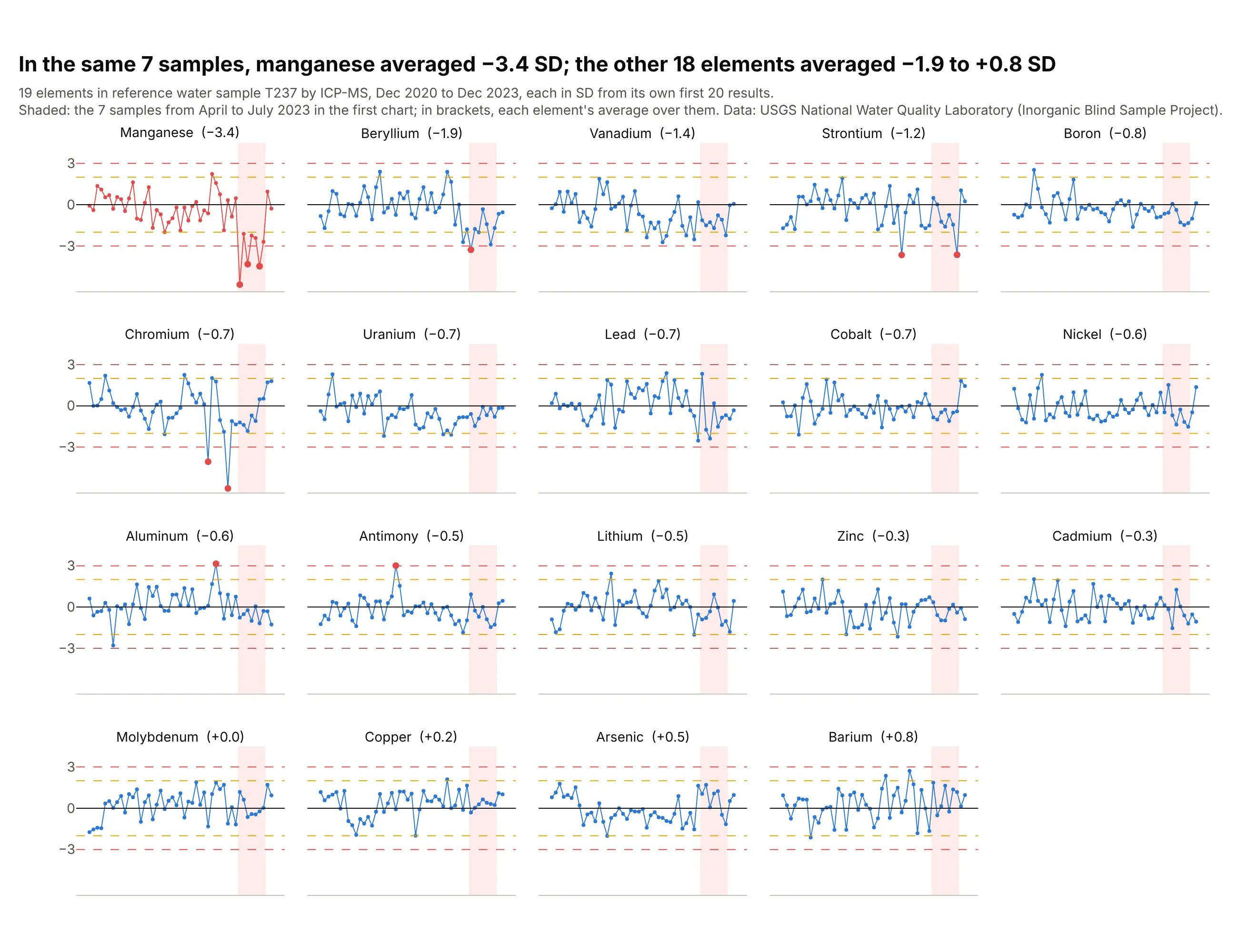
On the 7 samples from April to July 2023 where manganese dropped below −2 SD, it averaged −3.4 SD, while the 18 other elements measured in the same samples averaged between −1.9 and +0.8 SD. The problem was mostly manganese's, not the whole instrument's, which tells the lab where to look. Beryllium (−1.9) and vanadium (−1.4) also ran low, so the lab would check the shared parts of the method too. Data: USGS National Water Quality Laboratory, Inorganic Blind Sample Project.

Tip: sort the panels by how far each element moved in the period of interest, so the outlier sits in the top-left corner.

7. Vanadium again: why the lines stay fixed

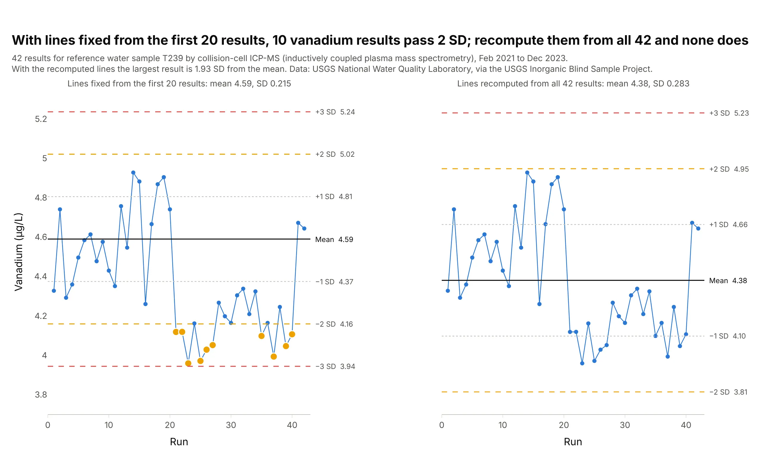
If the lab recomputes the mean and SD from all 42 vanadium results, shift included, the mean drops from 4.59 to 4.38 µg/L, the SD grows from 0.215 to 0.283, and the largest result is only 1.93 SD from the mean. No result is beyond 2 SD, where the fixed lines show 10. The shift is built into the lines, which is why labs set them from a baseline and keep them until a new lot starts. Data: USGS National Water Quality Laboratory, Inorganic Blind Sample Project.

Tip: when you must update the lines, show the old and new ones together for a few weeks and write down why, so a drift can't hide inside the update.