Chris Parmer

November 4, 2026

Control Charts - A Complete Guide

TL;DR

A control chart plots a measurement of a process in time order with a center line and two control limits, usually 3 standard deviations either side, so you can tell the ordinary variation of a stable process from a change worth investigating.
Control charts are also known as Shewhart charts, process-behavior charts and SPC (statistical process control) charts, and are similar to line charts and run charts. They are often used next to Pareto charts, which rank the causes once a control chart has found a problem.
Pick the chart by the data: X-bar and R charts for small samples of a measurement, individuals and moving range (I-MR) charts for one value at a time, p charts for the share of defective items and c or u charts for counts of defects. A run chart, with a median and no limits, is the simpler version that hospitals use.
You can make a control chart with Plotly from a go.Scatter trace, horizontal lines for the center and the limits, and a second trace for the points outside them. A short helper function is below.

What is a control chart?

Control charts look like this:

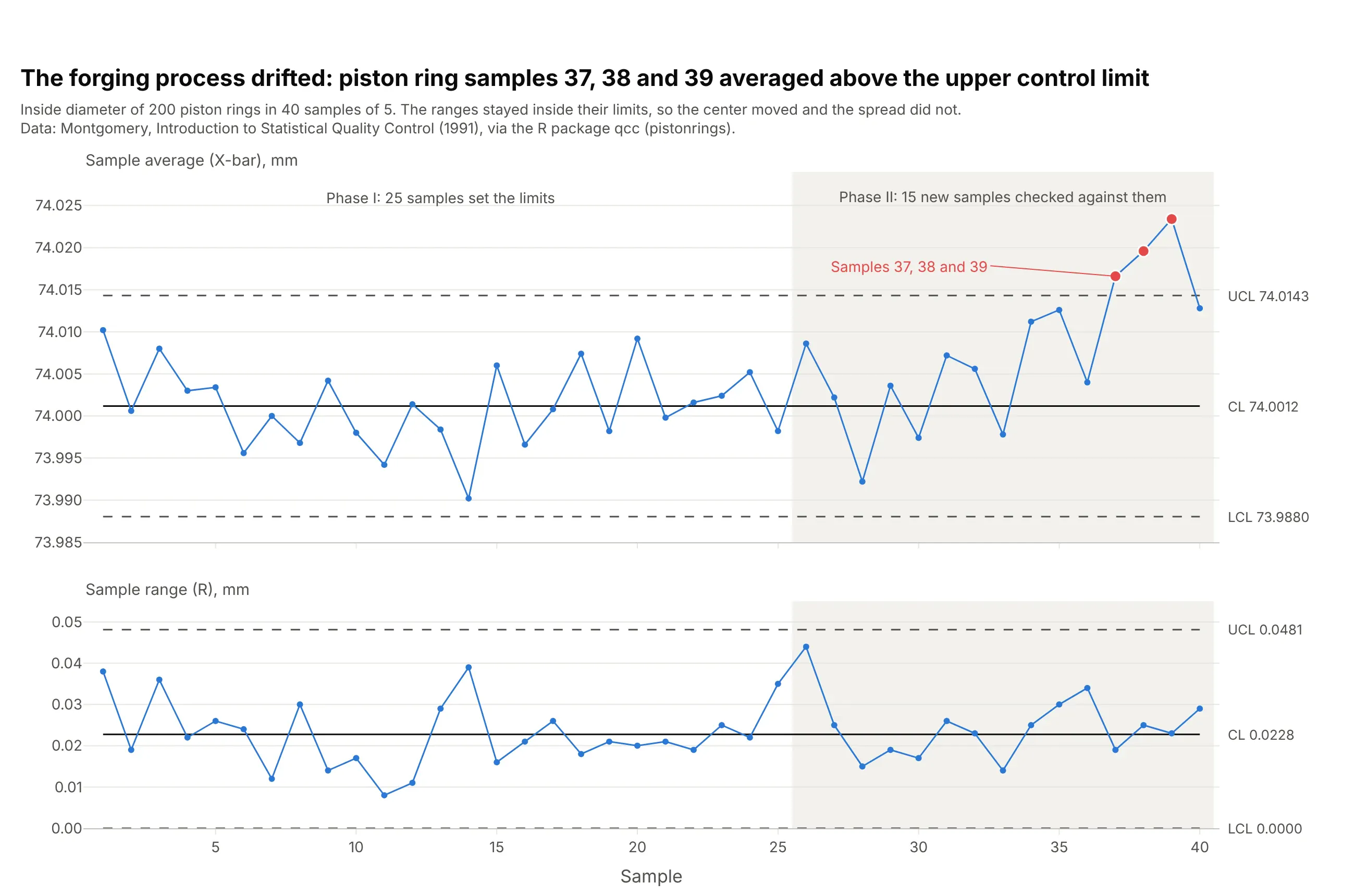
X-bar and R control charts of 40 samples of 5 forged piston rings: in the top panel sample averages wander around a center line of 74.0012 mm between dashed limits at 73.9880 and 74.0143, until samples 37, 38 and 39 in the shaded phase II rise above the upper limit in red; in the bottom panel every sample range stays below its upper limit of 0.0481

Data: Montgomery, Introduction to Statistical Quality Control (1991), via the R package qcc (pistonrings).

How do you read a control chart? In the example above, notice these things:

Each point in the top panel is the average inside diameter of a sample of 5 piston rings, in the order they were forged. The bottom panel shows each sample's range, the gap between its largest and smallest ring.
The solid line is the center, 74.0012 mm, and the dashed lines are the control limits, 73.9880 and 74.0143 mm. They come from the first 25 samples, when the process was considered stable, and say how far a sample average can wander by chance alone.
Points inside the limits are common-cause variation, so nobody should adjust the machine for them. Samples 37, 38 and 39 are above the upper limit, which signals that something changed in the forging process.
The ranges all stay below their limit of 0.0481 mm, so the spread of the rings didn't change. The center moved, and the spread did not.

It's often used for charts like these:

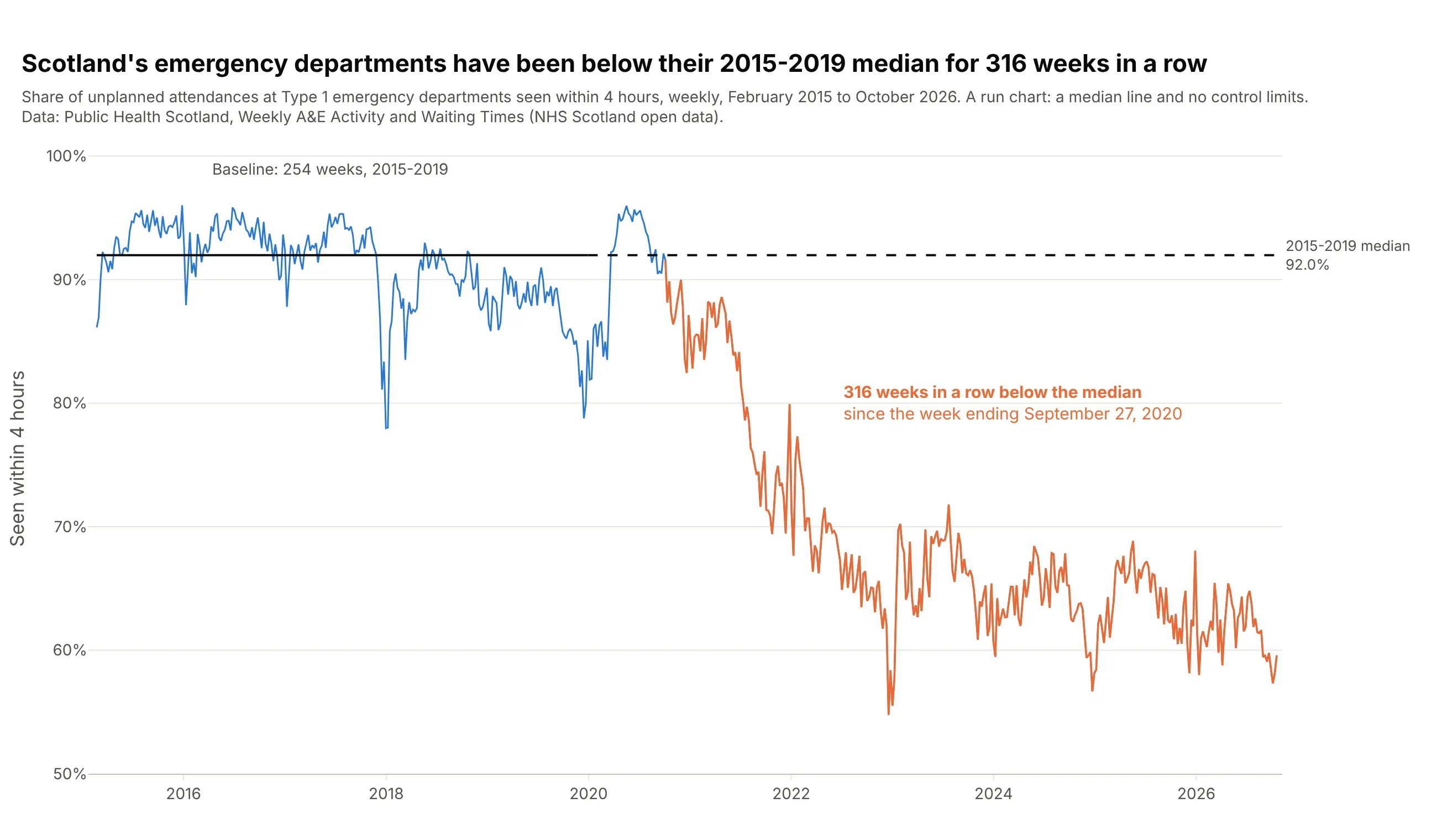
Run chart of the weekly share of patients seen within 4 hours at Scotland's emergency departments, 2015 to 2026: blue weeks around a solid median of 92.0% for 2015-2019, then an orange run that falls from about 90% in 2020 to about 60% in 2026, every week below the dashed median since September 27, 2020

Quality improvement in hospitals. Scotland's emergency departments have seen a smaller share of patients within 4 hours than their 2015-2019 median of 92.0% for 316 weeks in a row, which a run chart shows with nothing more than a median line. Data: Public Health Scotland, Weekly A&E (accident and emergency) Activity and Waiting Times.

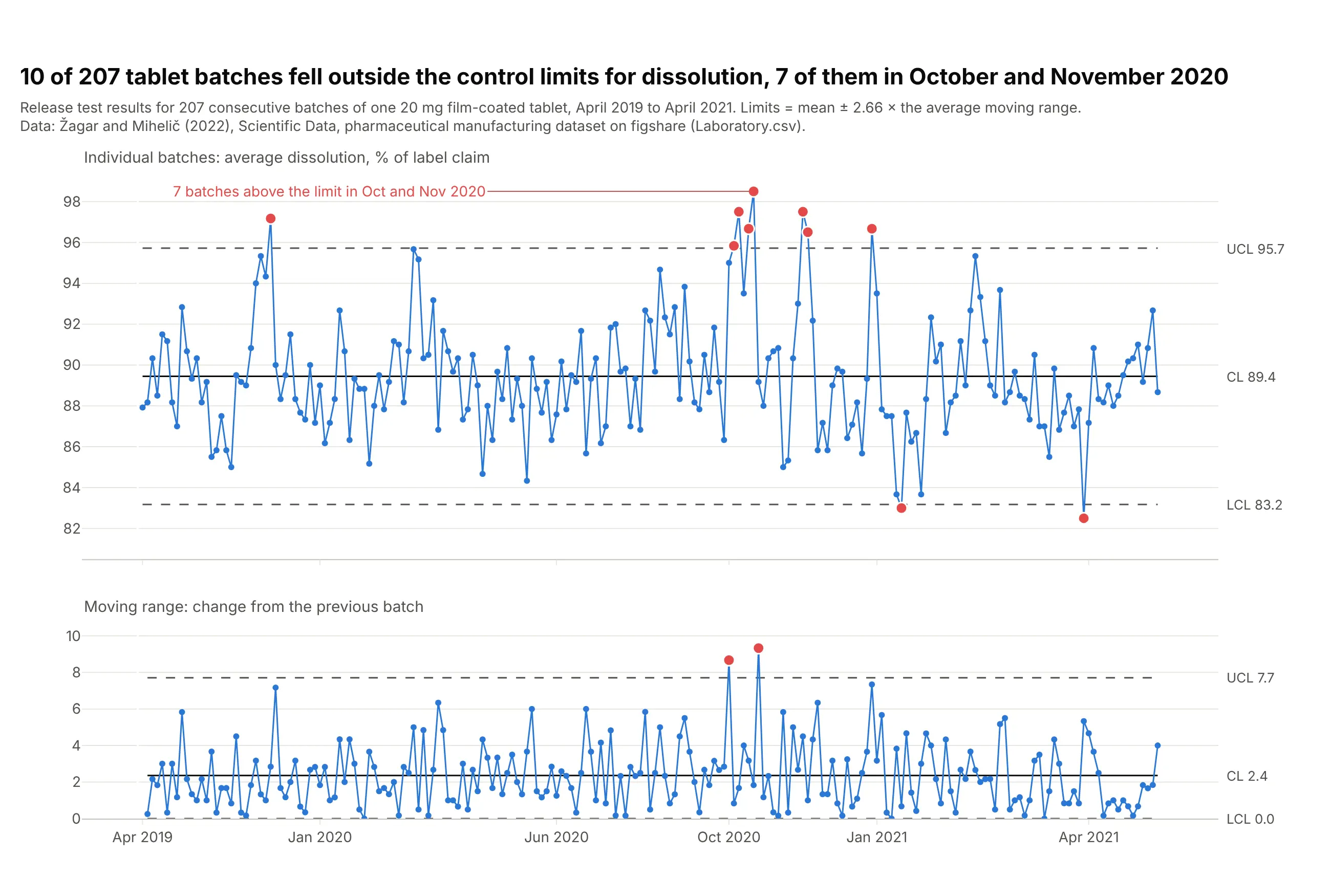
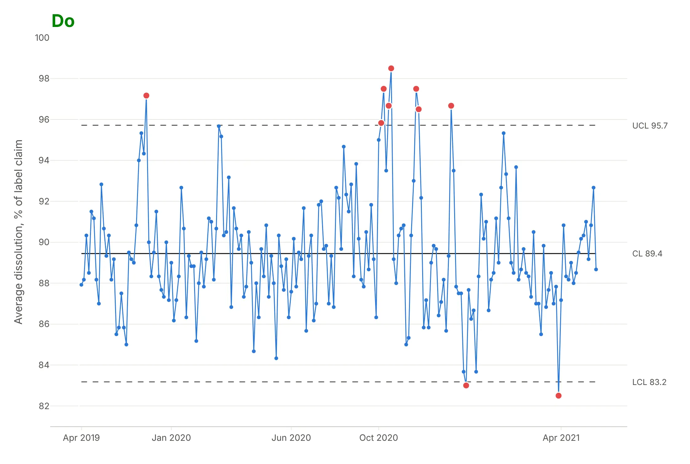
Individuals and moving range chart of average dissolution for 207 consecutive batches of a 20 mg tablet, April 2019 to April 2021: batches vary between dashed limits at 83.2% and 95.7%, with red batches above the upper limit clustered in October and November 2020 and two below the lower limit in 2021

Batch release in pharma. 10 of 207 tablet batches fell outside the limits of an individuals chart of dissolution, 7 of them in October and November 2020, a cluster that suggests something changed in the process that autumn. Data: Žagar and Mihelič (2022), Scientific Data, figshare.

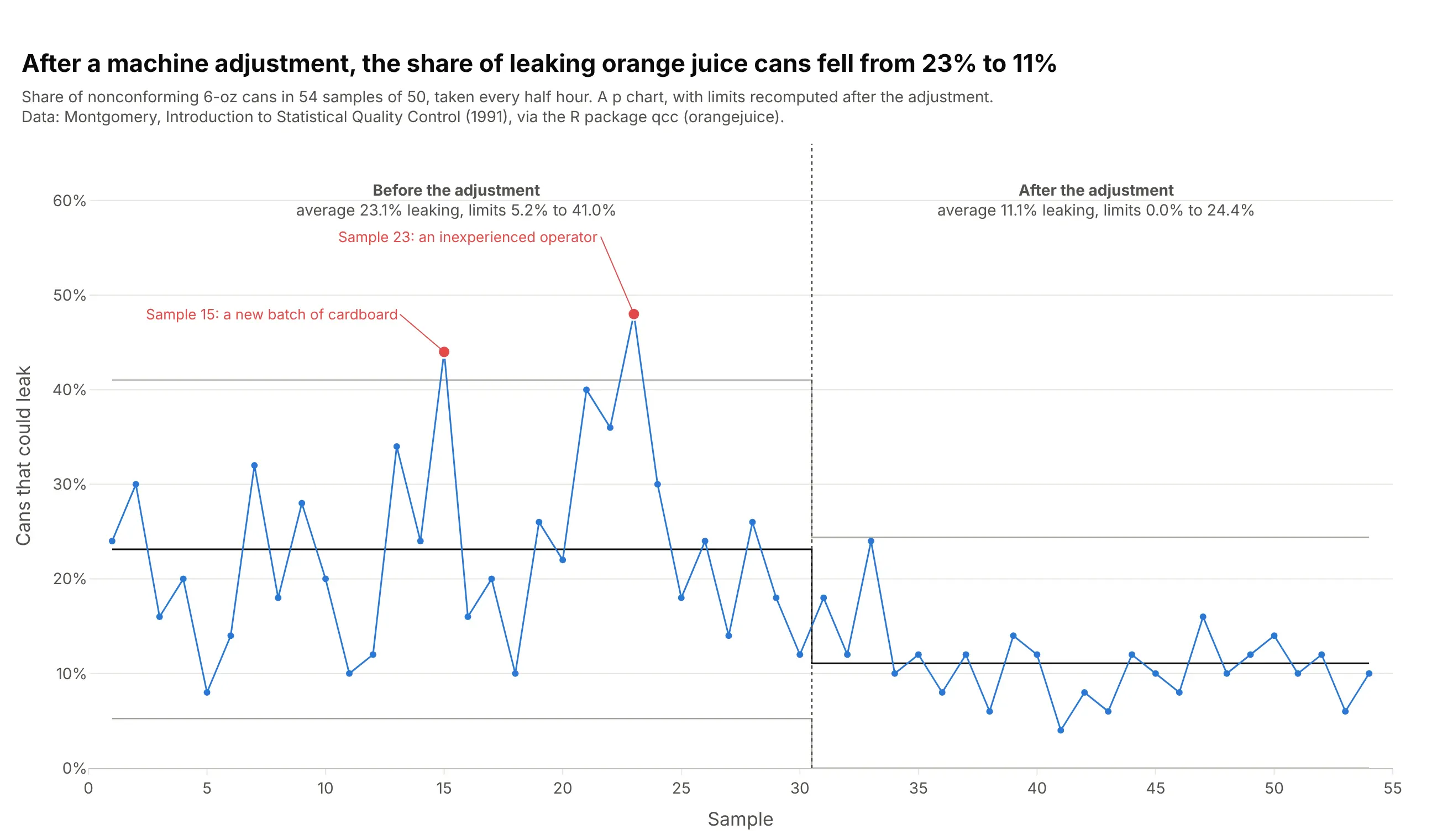
p chart of the share of leaking orange juice cans in 54 samples of 50: before a machine adjustment the share averages 23.1% between limits of 5.2% and 41.0%, with samples 15 and 23 above the limit and labeled with their causes; after the adjustment it averages 11.1% under a limit of 24.4%

Defective items in manufacturing. A p chart shows the share of leaking orange juice cans fell from 23% to 11% after a machine adjustment, and the two samples above the earlier limit both had a known cause. Data: Montgomery (1991), via the R package qcc (orangejuice).

A short history

Walter Shewhart invented the control chart at Western Electric and Bell Labs in the 1920s. On May 16, 1924 he wrote a one-page memo with a diagram that his manager George Edwards later said "we would all recognize today as a schematic control chart" (Wikipedia), and he published the method in the Bell System Technical Journal in 1926 (Shewhart 1926) and in his 1931 book Economic Control of Quality of Manufactured Product. His idea was that every process varies, and that management should act only on the variation that has an assignable cause. W. Edwards Deming came across Shewhart's work in 1924 or 1925 and became its foremost champion, including in Japan after the war (Wikipedia). Western Electric's 1956 Statistical Quality Control Handbook added the zone rules below, and healthcare improvement teams later adopted the simpler run chart (Perla, Provost and Murray 2011).

How control limits are calculated

A control chart's limits look like simple horizontal lines, but they carry most of its logic. They answer one question: how far can this process wander by chance alone? Everything below is about estimating that distance well, and about the few cases where the lines are meant to move.

Sigma, and why the limits sit at 3 sigma

Sigma (σ) is the standard deviation, the typical distance between a measurement and the average. For a stable process whose values follow a normal distribution, about 68% of points fall within 1 sigma of the mean, 95% within 2 sigma and 99.7% within 3 sigma:

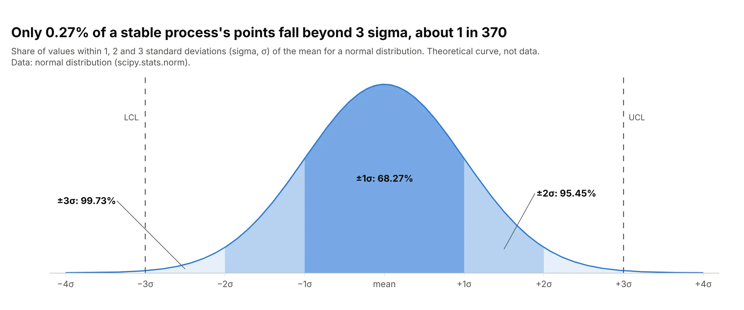
A normal curve with the areas within 1, 2 and 3 standard deviations of the mean shaded and labeled 68.27%, 95.45% and 99.73%, and dashed lines at minus and plus 3 sigma labeled LCL and UCL

Data: the normal distribution (theoretical, not data).

Shewhart put the upper control limit (UCL) and lower control limit (LCL) at 3 sigma from the center line (CL) because that makes false alarms rare. Only 0.27% of points from a stable normal process land beyond them, so the 3-sigma rule alone raises a false alarm about once every 370 points (the NIST/SEMATECH e-Handbook of the US National Institute of Standards and Technology, NIST, gives 371). Narrower limits would catch changes sooner but would send people chasing causes that aren't there.

Sample ranges and the average moving range

The sigma on a control chart is estimated from short-term variation, the spread you see over a short stretch of time. For an X-bar and R chart that is the sample range, the largest minus the smallest value in each sample: the piston ring samples have an average range of 0.0228 mm, and the X-bar limits are the grand mean plus and minus 0.577 times that.

When there is only one measurement per point, as with one test result per tablet batch, the chart uses the moving range instead. A moving range is the absolute difference between each measurement and the one before it, and the average moving range is the mean of all those differences:

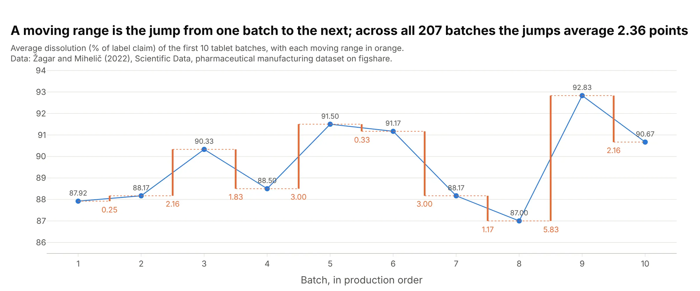
The first 10 tablet batches as a line of dots labeled with their dissolution, 87.92, 88.17, 90.33 and so on, with an orange vertical bar between each pair of neighbors labeled with the jump between them: 0.25, 2.16, 1.83, 3.00, 3.00, 0.33, 3.00, 1.17, 5.83 and 2.16

Data: Žagar and Mihelič (2022), Scientific Data, figshare.

The first three batches dissolved 87.92%, 88.17% and 90.33%, so their moving ranges are 0.25 and 2.16. Across all 207 batches there are 206 moving ranges, and they average 2.36. The limits are the mean, 89.45%, plus and minus 2.66 times 2.36, which gives 83.2% and 95.7%. The 2.66 is 3 divided by 1.128, where 1.128 is the constant d2 that converts the average range of two points into a standard deviation (NIST/SEMATECH e-Handbook, 6.3.2.2). So 2.36 / 1.128 = 2.09 is the estimated sigma, and the limits are 3 sigma from the mean.

Fixed limits: phase I and phase II

The moving range slides along the series one pair of batches at a time, but the limits don't move with it. The ranges are averaged over a fixed baseline, and the limits are drawn as fixed lines. In phase I you set the limits from a baseline period that looks stable, usually 20 to 25 points or more (the first 25 piston ring samples). In phase II you keep those limits fixed and plot each new point against them, which is how samples 37 to 39 showed up as a change.

You recalculate the limits on purpose, after a deliberate change to the process. In the orange juice example, the limits before the machine adjustment were 5.2% to 41.0% leaking cans around 23.1%, and after it 0% to 24.4% around 11.1%. The chart is split at the adjustment, and each part has its own fixed limits.

When the limits do move

Three kinds of chart have limits that change from point to point, each for a reason.

Limits that depend on sample size. On p and u charts, each point's limits depend on how much it is based on. A quarter with fewer patients has a noisier infection rate, so its limits are wider:

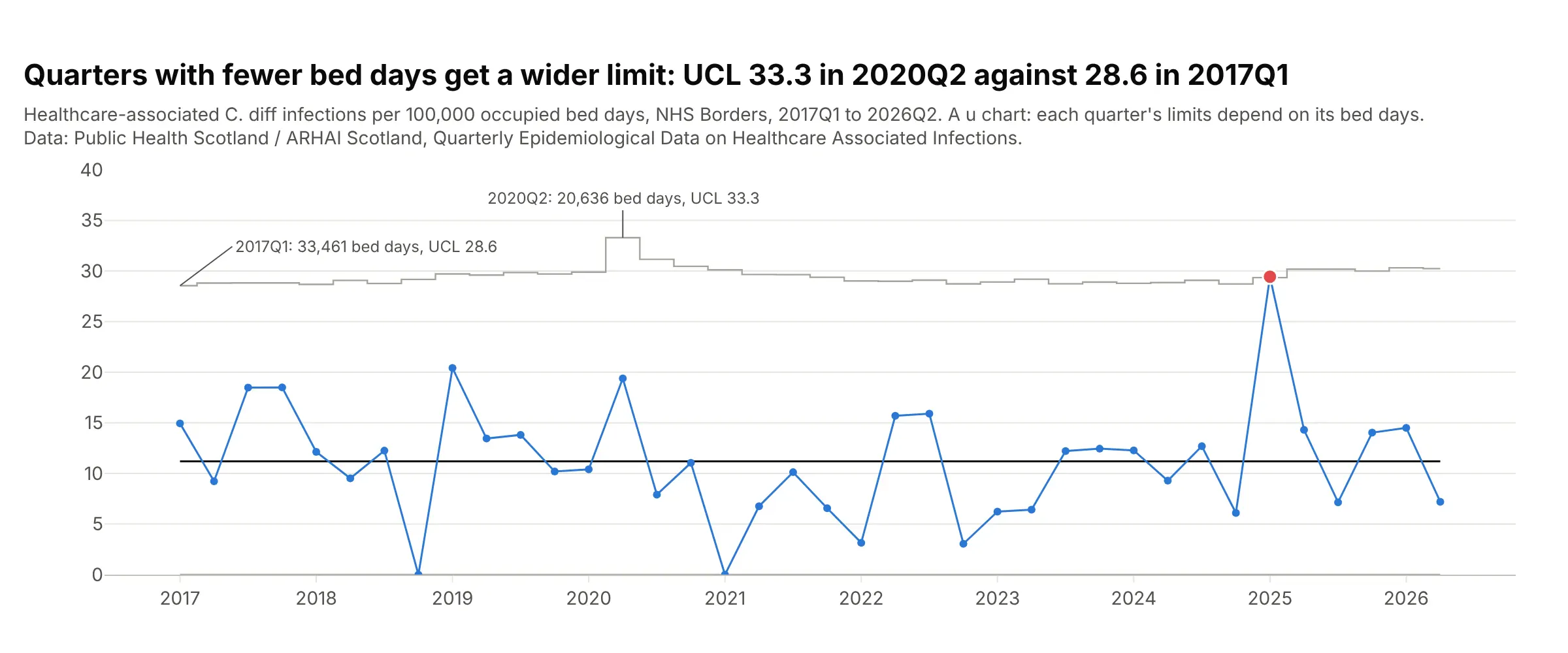
u chart of NHS Borders' quarterly C. diff infections per 100,000 bed days, 2017 to 2026, with a stepped upper limit near 29 to 30 that jumps to 33.3 in 2020Q2, the quarter with the fewest bed days, and one red quarter in 2025Q1 just above its limit

Data: Public Health Scotland / ARHAI Scotland (Antimicrobial Resistance and Healthcare Associated Infection), Quarterly Epidemiological Data on Healthcare Associated Infections.

For NHS Borders, one of the regional boards of Scotland's National Health Service (NHS), the healthcare-associated C. diff (Clostridioides difficile) upper limit was 28.6 infections per 100,000 bed days in 2017Q1, with 33,461 bed days, and 33.3 in 2020Q2, with 20,636. The center line stays at the overall rate of 11.2.

EWMA limits at the start. An EWMA (exponentially weighted moving average) chart averages each point with the ones before it, so its first values are based on less history and its limits start narrow. They widen over the first few points and then settle at a fixed width:

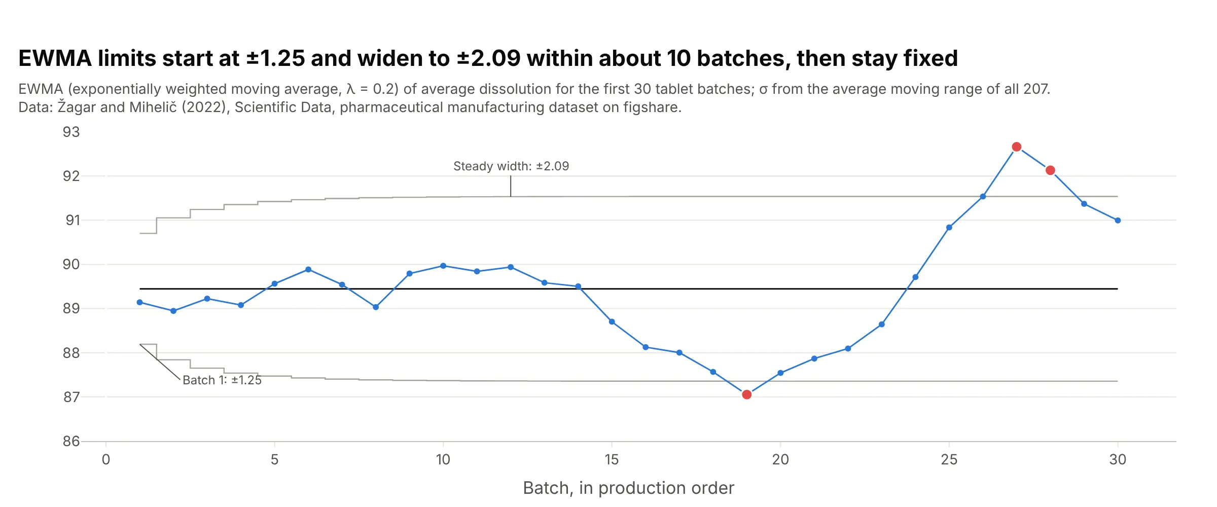
EWMA of the first 30 tablet batches with stepped limits that start at plus or minus 1.25 around the center and widen to a steady plus or minus 2.09 by about batch 10

Data: Žagar and Mihelič (2022), Scientific Data, figshare.

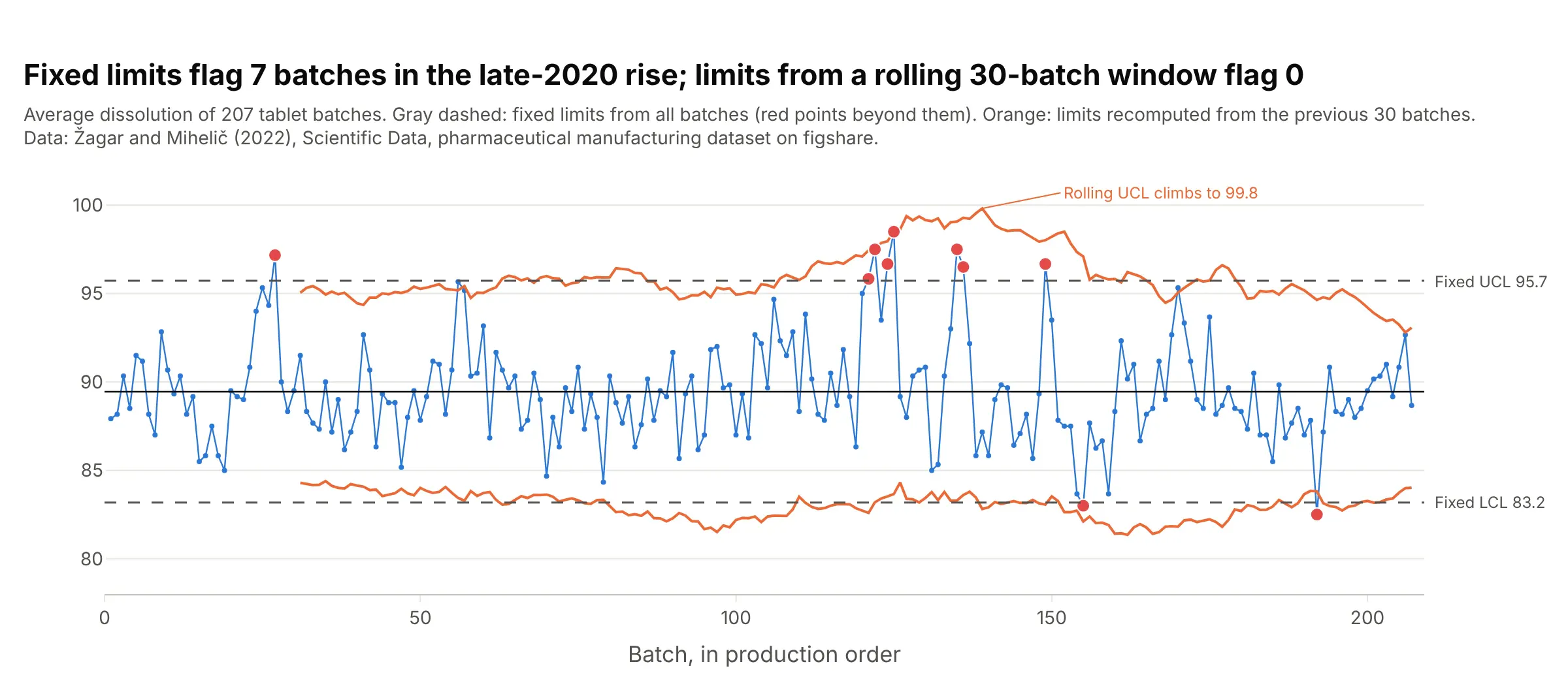
Rolling limits, which SPC avoids. Some dashboards recompute the limits from a rolling window, such as the last 30 points. That makes the limits follow the process, which means they also follow the change you wanted to catch:

The 207 tablet batches with fixed dashed limits at 83.2 and 95.7 and orange rolling limits from the previous 30 batches; during the late-2020 rise the rolling upper limit climbs to 99.8, above every batch, while seven batches in red are beyond the fixed limit

Data: Žagar and Mihelič (2022), Scientific Data, figshare.

Between batches 100 and 150, fixed limits flag 7 batches. Limits from the previous 30 batches flag none, because the rolling upper limit climbs to 99.8% as the high batches enter the window. That's why statistical process control (SPC) keeps limits fixed and recalculates them only on purpose.

Why short-term spread, not the overall standard deviation

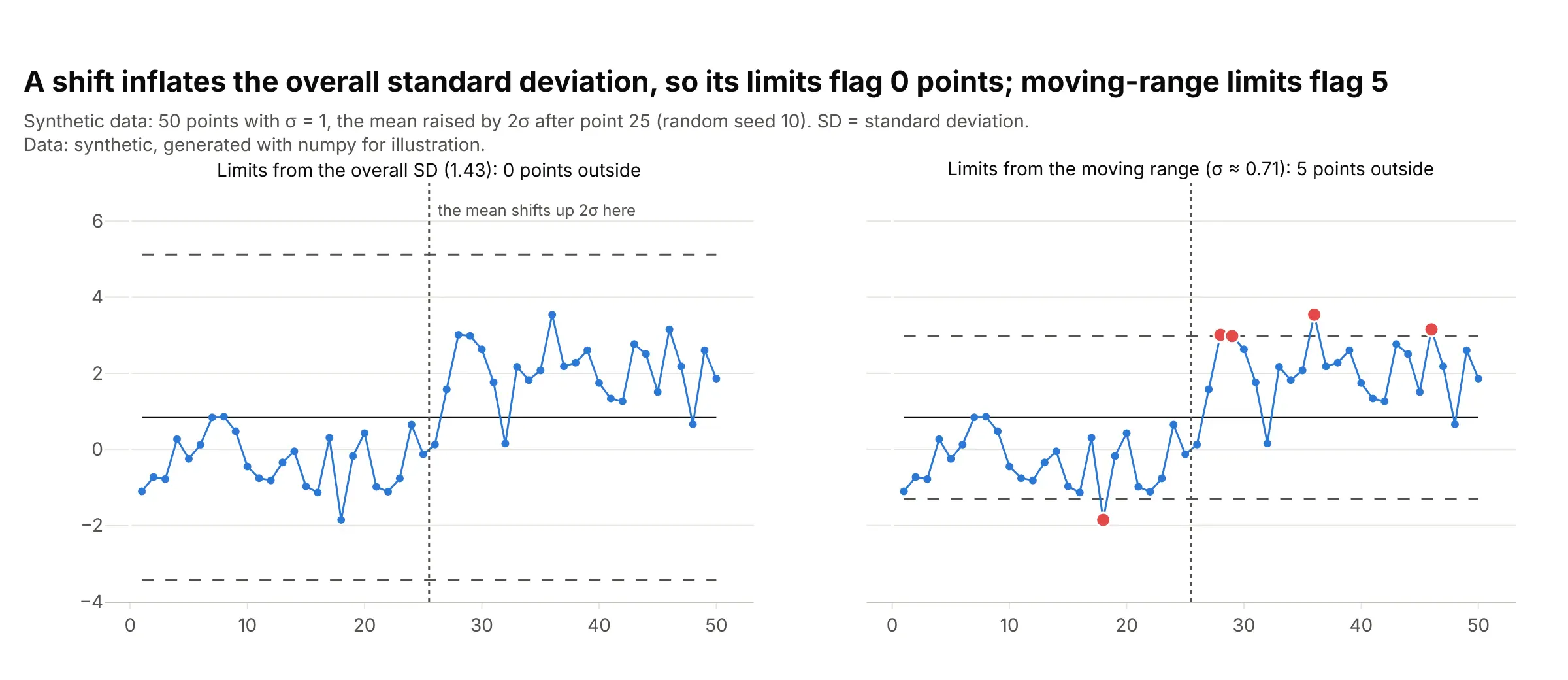
The overall standard deviation of all the data includes every shift the process went through, so it is inflated by exactly the changes the chart is meant to catch. Short-term spread, from moving ranges or within-sample ranges, mostly measures the noise from one point to the next. This synthetic example has 50 points whose mean jumps by 2 sigma halfway through:

Two panels of the same 50 synthetic points with a jump in the mean after point 25: on the left, limits from the overall standard deviation of 1.43 are so wide that no point falls outside; on the right, limits from the moving range, sigma about 0.71, flag 5 points in red

Data: synthetic, generated with numpy (seed 10) for illustration.

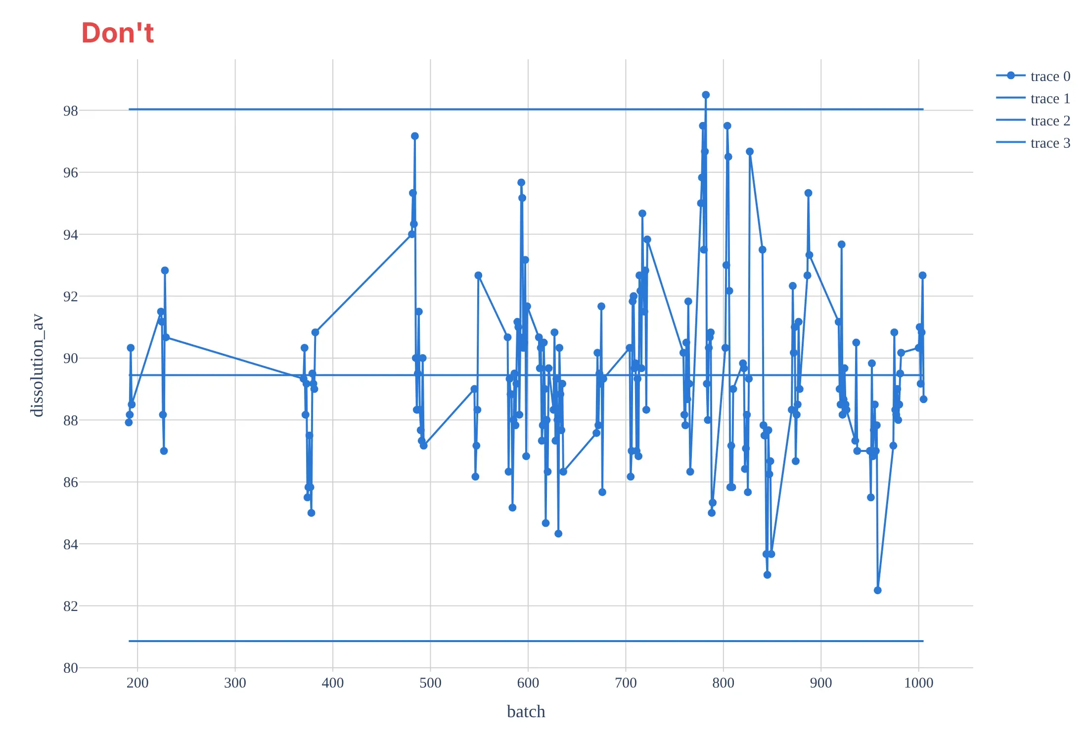
Limits from the overall standard deviation (1.43) flag no point at all. Limits from the moving range (sigma about 0.71) flag 5, four of them after the jump and one false alarm before it. The tablet data shows the same thing: limits at 3 overall standard deviations (2.86) run from 80.9% to 98.0% and only 1 batch falls outside, against 10 with the moving-range limits, which is the mistake in the Don't chart below.

Control limits are not specification limits

Control limits describe what the process does, computed from its own data. Specification limits describe what the customer or a regulator requires, such as a minimum dissolution for a tablet. A process can be in control and still make product out of spec, or out of control while every unit is within spec, so don't draw one in place of the other.

The rules for out-of-control points

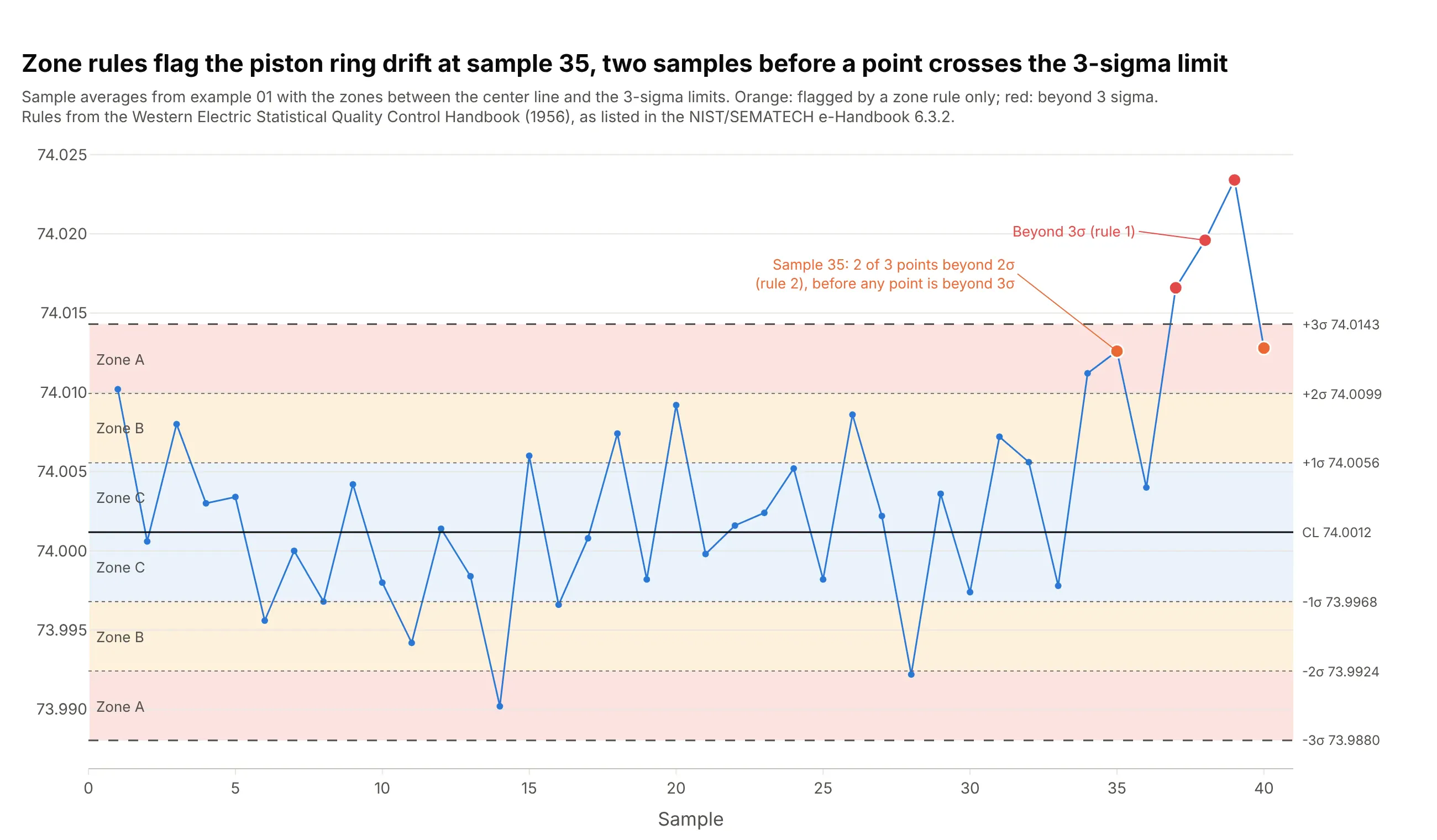
A point beyond 3 sigma is the first rule. The Western Electric rules add three more that catch smaller shifts by splitting the area inside the limits into zones at 1 and 2 sigma:

One point beyond 3 sigma (zone A and beyond).
Two of three points in a row beyond 2 sigma on the same side.
Four of five points in a row beyond 1 sigma on the same side.
Eight points in a row on the same side of the center line.

On the piston ring data, rule 2 fires at sample 35, two samples before a point crosses the limit:

The piston ring X-bar chart with zones A, B and C shaded between the center line and the 3-sigma limits on each side: samples 35 and 40 in orange are flagged by the zone rules, and samples 37 to 39 in red are beyond 3 sigma; sample 35 is labeled two of three points beyond 2 sigma

Data: the 40 piston ring samples from the chart above; rules as listed in the NIST/SEMATECH e-Handbook, 6.3.2.

More rules mean more false alarms. With the 3-sigma rule alone, a stable process gives a false signal every 371 points on average; with the four Western Electric rules, about every 92 points (NIST). The Nelson rules (Nelson 1984) are a set of eight that adds trends (six points in a row rising or falling), oscillation (14 alternating up and down) and too little variation (15 points in a row within 1 sigma). Pick one rule set, say which one on the chart, and use it every time.

Which control chart to use, and run charts

Each kind of data has its own chart, because the limits come from a different formula. Here is one example of each.

1. X-bar and R chart

For measurements taken in small samples (2 to 10), such as 5 rings every hour. Plot each sample's average (X-bar) and its range:

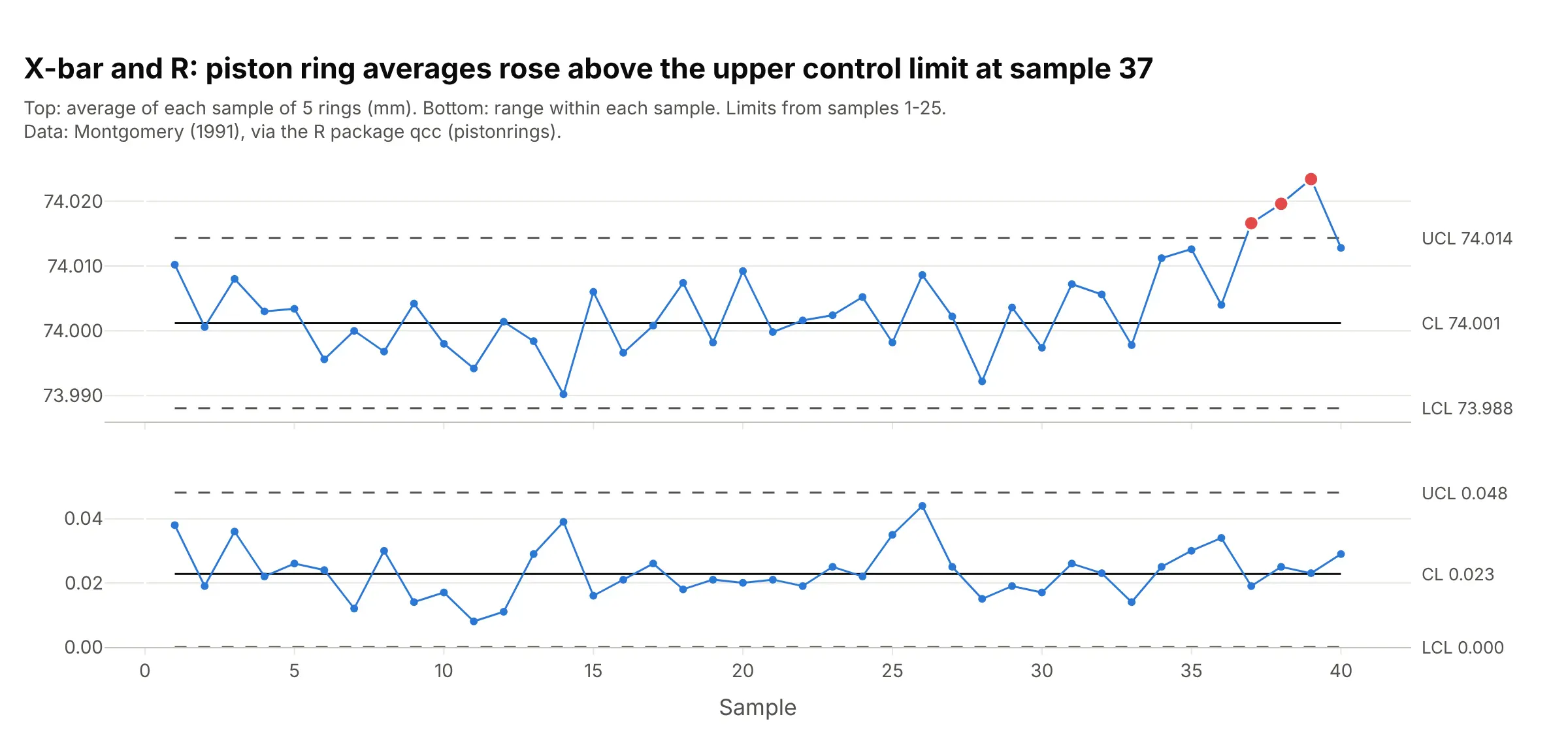
Compact X-bar and R charts of the 40 piston ring samples: averages cross the upper limit of 74.014 mm at samples 37, 38 and 39, while every range stays below its limit of 0.048

Data: Montgomery (1991), via the R package qcc (pistonrings). The full chart is the first one in this guide.

2. X-bar and S chart

The same idea for larger samples, with each sample's standard deviation (S) in place of its range:

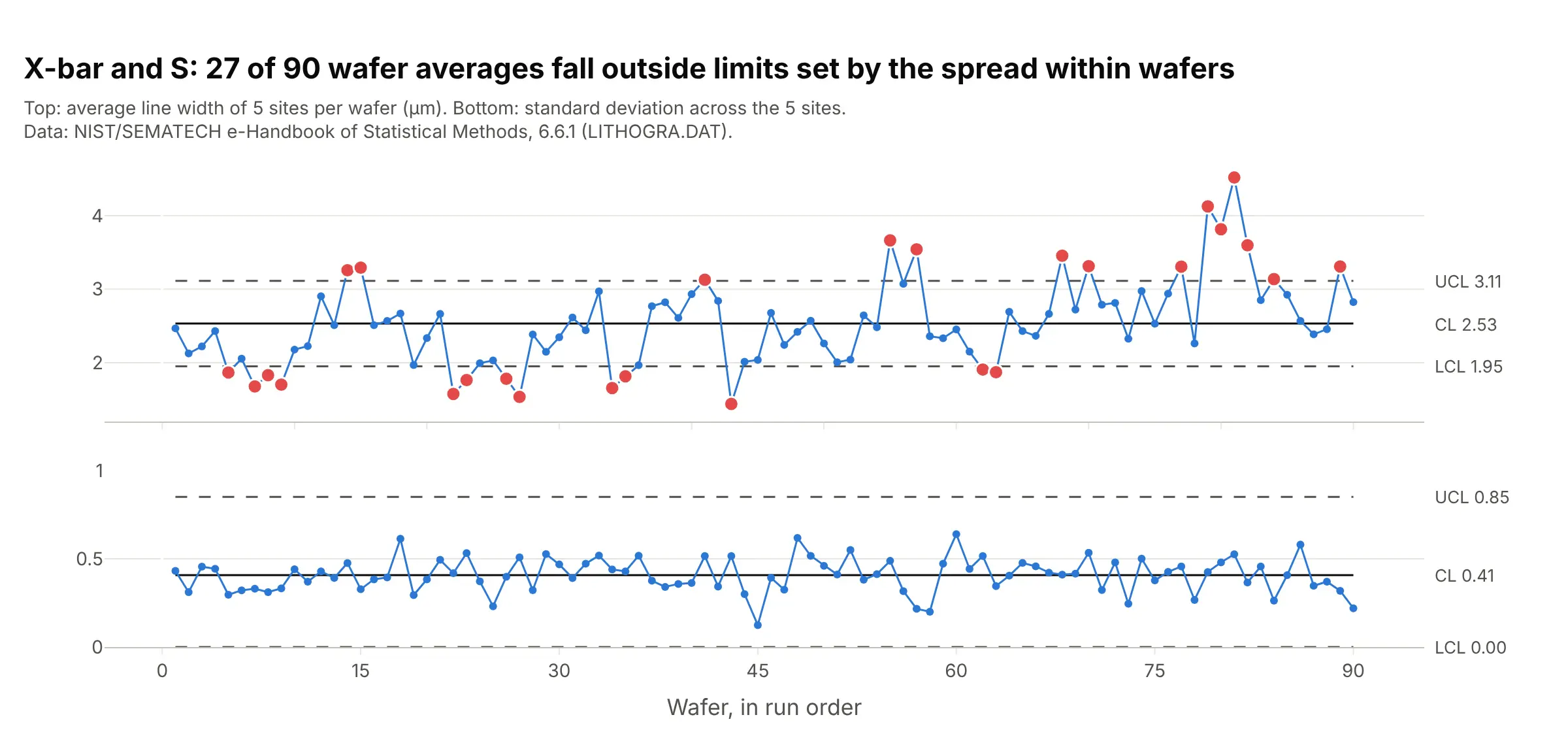
Compact X-bar and S charts of 90 wafers: 27 wafer averages in red fall outside X-bar limits of 1.95 and 3.11 µm, and every wafer's standard deviation stays below its limit of 0.85

Data: NIST/SEMATECH e-Handbook of Statistical Methods, 6.6.1. The full example is "Line width on silicon wafers" under More control chart examples.

3. Individuals and moving range (I-MR) chart

For one measurement at a time, such as one test result per batch, with limits at the mean plus and minus 2.66 times the average moving range, as worked through above. It is also called an XmR chart:

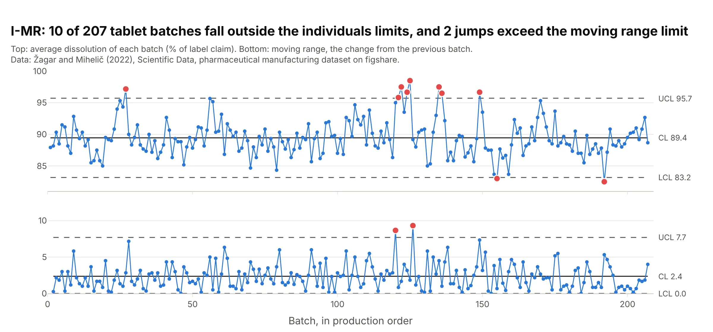
Compact I-MR chart of 207 tablet batches: 10 batches in red outside individuals limits of 83.2% and 95.7%, and 2 moving ranges above their limit of 7.7

Data: Žagar and Mihelič (2022), Scientific Data, figshare. The full chart is under "What is a control chart?".

4. p chart and np chart

For defective items: the p chart plots the share of defective items in each sample, with limits that widen for smaller samples, and the np chart plots the count when every sample has the same size:

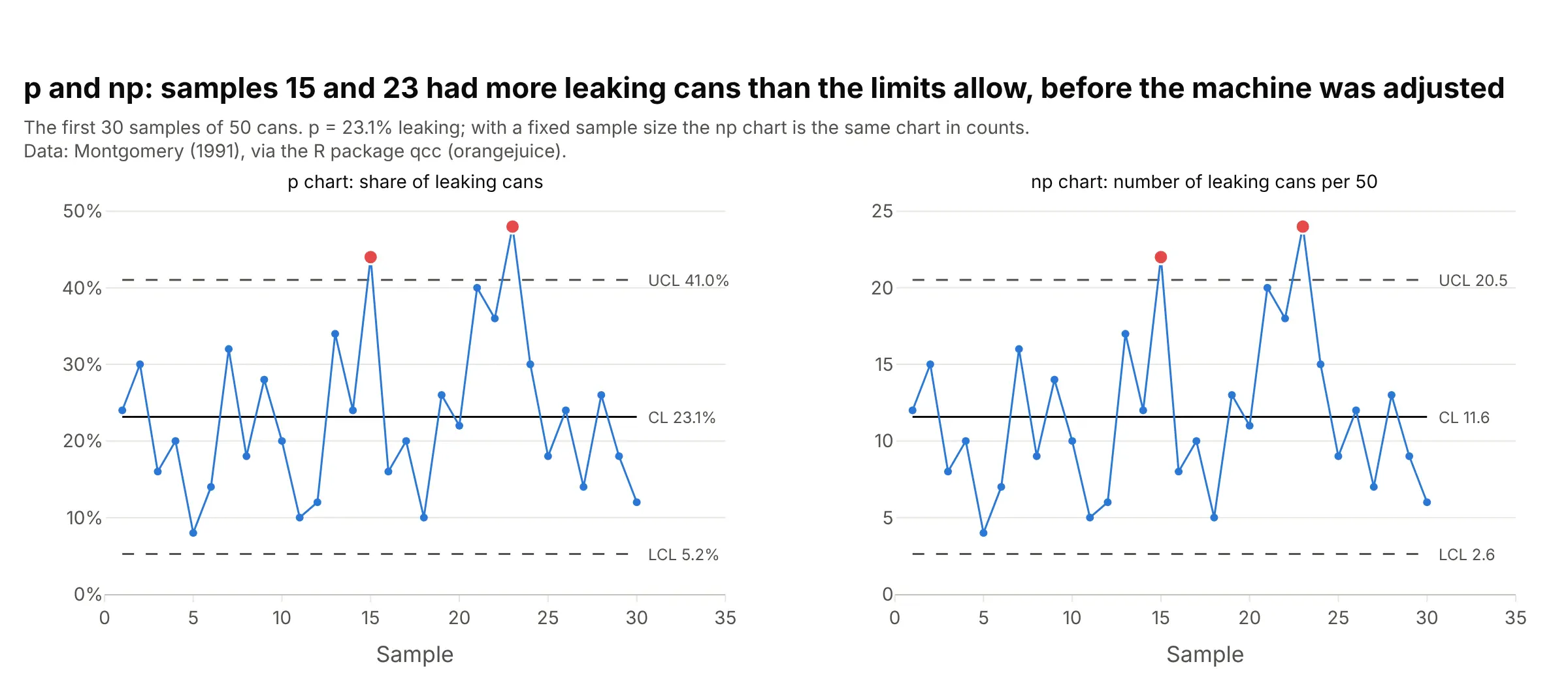
A p chart and an np chart of the first 30 orange juice samples side by side, identical in shape: samples 15 and 23 above the limits of 41.0% and 20.5 cans

Data: Montgomery (1991), via the R package qcc (orangejuice). The full chart, with the limits after the adjustment, is under "What is a control chart?", and the Semmelweis example under More control chart examples is a p chart with a different sample size every month.

5. c chart and u chart

For counts of defects: the c chart counts them per inspection unit of a fixed size, and the u chart divides by a varying amount of exposure, such as 100,000 bed days:

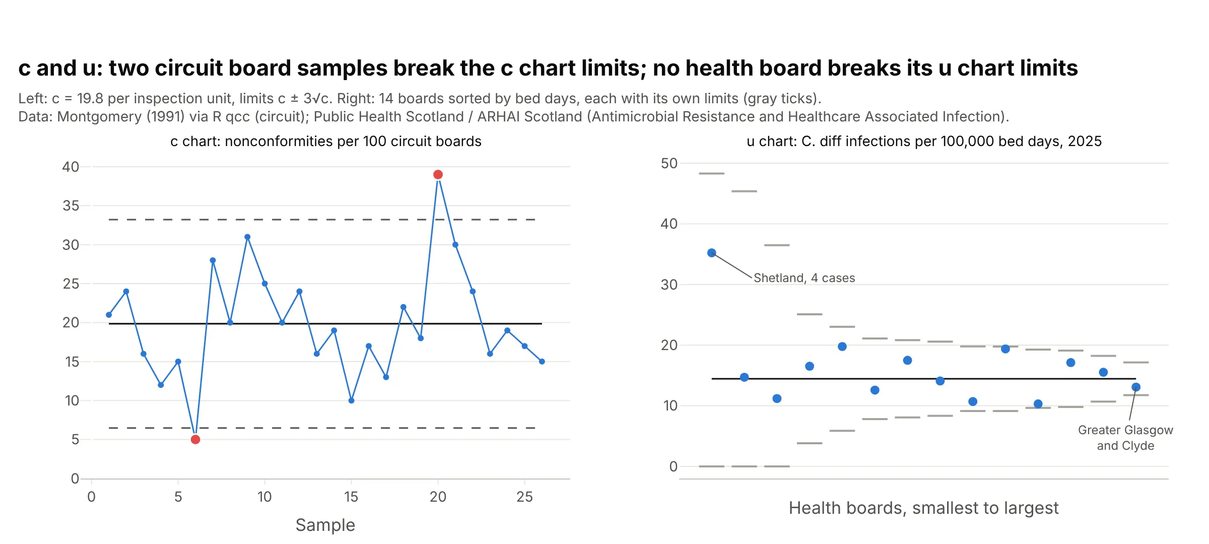
A c chart of 26 circuit board samples with samples 6 and 20 outside limits of 6.5 and 33.2, next to a u chart of 14 health boards whose gray limit ticks narrow from the smallest board to the largest, with every board inside

Data: Montgomery (1991) via the R package qcc (circuit); Public Health Scotland / ARHAI Scotland. The full examples are "Nonconformities on printed circuit boards" and "Hospital infection rates across 14 health boards" under More control chart examples.

6. EWMA and CUSUM charts

An EWMA chart plots a running weighted average that gives each new point a share λ of the weight, and a CUSUM (cumulative sum) chart adds up each point's distance from the center, minus a small allowance k, until the sum crosses a decision limit h. Both pick up small, sustained shifts sooner than a Shewhart chart:

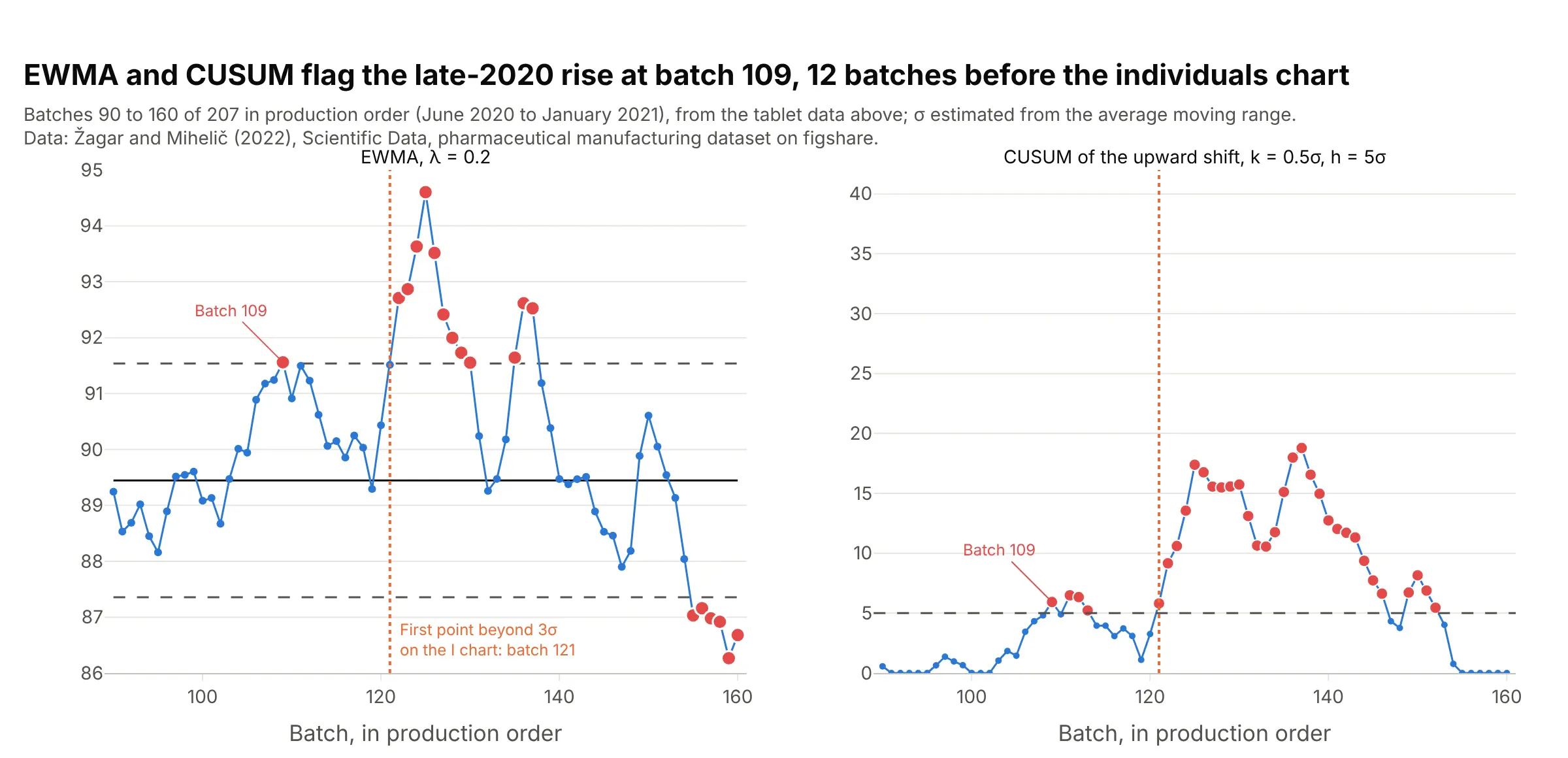
EWMA and CUSUM charts of tablet batches 90 to 160: both signal at batch 109, while a dotted orange line marks batch 121, the first point beyond 3 sigma on the individuals chart

Data: Žagar and Mihelič (2022), Scientific Data, figshare. Both flag the late-2020 rise at batch 109 (in production order), 12 batches before the first point beyond 3 sigma on the individuals chart. The alternatives figure below draws them over all 207 batches.

7. Run chart

The data in time order with a median line and no limits. Its rules count runs instead of sigmas: a run longer than about log2(n) + 3 points, or too few crossings of the median, signals a shift (qicharts2). It needs no distribution and no sigma, which is why hospital improvement teams start with it, and it becomes a control chart once you add limits:

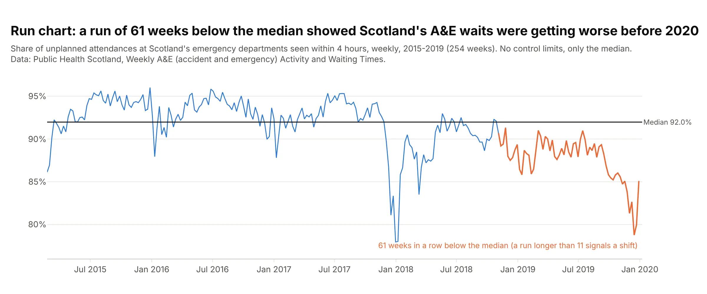
Run chart of Scotland's weekly A&E waiting times, 2015 to 2019, with a median of 92.0% and an orange run of 61 weeks below it from November 2018 to December 2019

Data: Public Health Scotland, Weekly A&E (accident and emergency) Activity and Waiting Times. With 254 weeks, any run longer than 11 signals a shift, and this one is 61 weeks. The full run chart to 2026 is under "What is a control chart?".

Alternatives to a control chart

Here's the same tablet batch data drawn six ways. Some are better for the question, some worse, some just different:

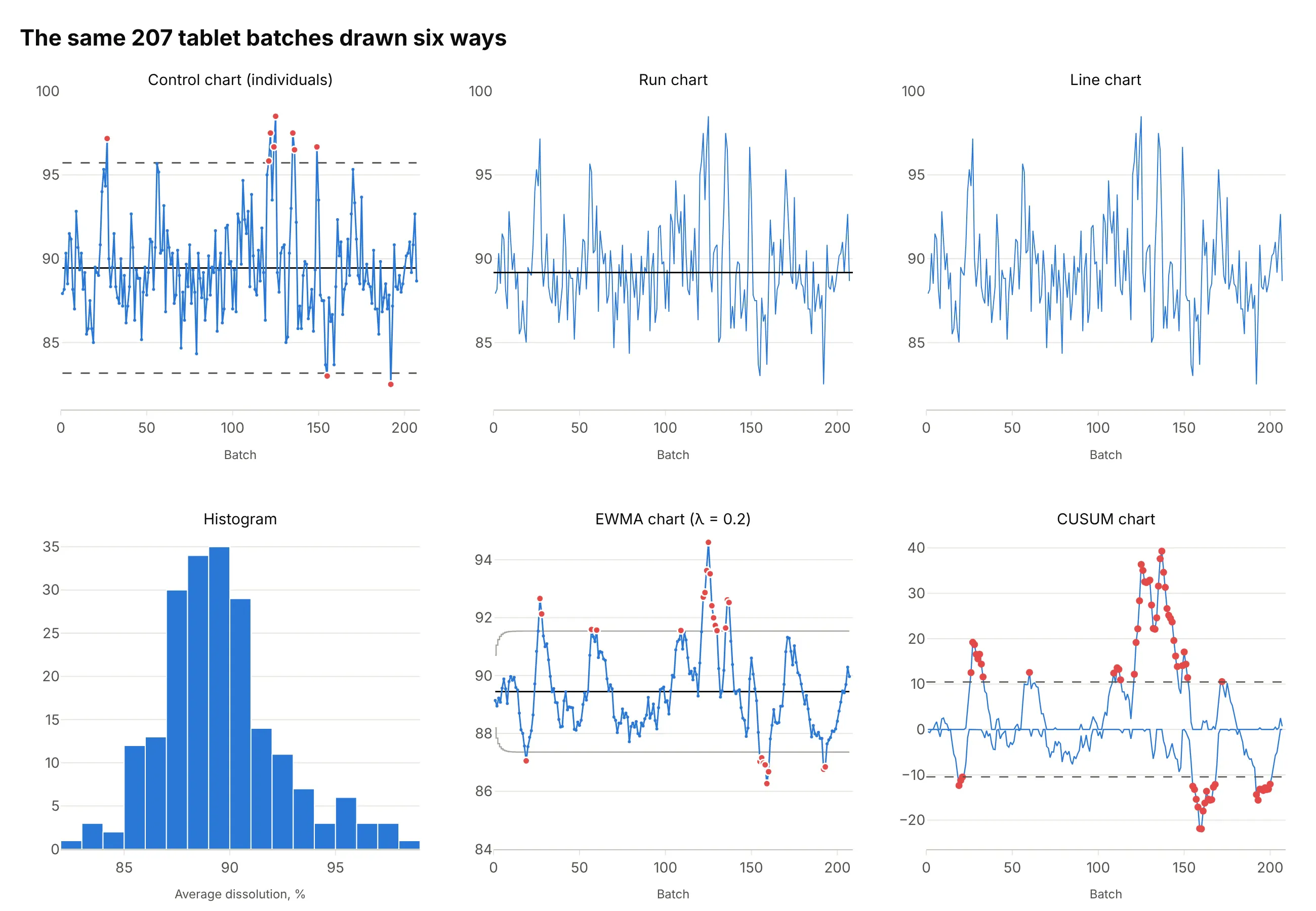
The 207 tablet batches drawn six ways: an individuals control chart with red points beyond the limits, a run chart with a median line, a plain line chart, a histogram with a long right tail, an EWMA chart with a smooth line that leaves its limits in late 2020 and early 2021, and a CUSUM chart whose upper sum climbs to about 39 in late 2020

Run chart (works too, for a first look). A median line and the runs rules need no sigma, and here they flag a shift because the line crosses the median 82 times where at least 87 are expected. They can't say which batches are unusual.
Line chart (worse). The same line without a reference leaves readers to guess which spikes matter, which is the problem a control chart was invented to solve.
Histogram (different). It shows the distribution and the long right tail for a capability study against specification limits, but it throws away the time order, so the October 2020 cluster disappears.
EWMA chart (better for small shifts). Averaging each batch with the ones before it smooths out noise, and 26 batches fall outside its limits, 12 of them in October and November 2020.
CUSUM chart (better for sustained shifts). Cumulative sums of the deviations from the mean show the process ran high through late 2020 and low in early 2021, which single points can't show. The scale, a sum of deviations, takes explaining.

When a control chart finds a problem, a Pareto chart of the defect causes is the usual next step, and a box plot of the measurements by machine, shift or supplier often shows where the variation comes from.

How to make a control chart

With AI

ChatGPT, Claude Code, GitHub Copilot, Cursor and other AI tools are excellent at writing Plotly code. Name Plotly in the prompt, and say which chart type, which samples set the limits and which rules to apply:

Make a plotly control chart from piston_rings.csv (columns: sample, diameter_mm, phase; 5 rings per sample).

- An X-bar chart on top and an R chart below with shared x, using go.Scatter with lines and markers.
- Limits from the phase I samples only: X-bar = grand mean +/- 0.577 x average range, R UCL = 2.114 x average range.
- Center line solid, limits dashed, each labeled with its value at the right.
- Points outside the limits as a second trace in red, and phase II shaded.
- Check: print the limits and the samples outside them.

With Plotly Studio

Plotly Studio is a desktop app where you point an AI at a dataset and it builds charts and a Dash app around your questions. Ask for a control chart the same way:

Show an individuals and moving range control chart of average dissolution by batch, limits from the average moving range, batches outside the limits in red with the batch number on hover, and a dropdown to pick the product.

Make a control chart in Python or JavaScript

This is the code AI tools write under the hood. Plotly has no dedicated control chart trace, so a control chart is a go.Scatter of the statistic, horizontal lines for the center and the limits, and a second trace for the points outside them. This helper returns a go.Figure, and every example in this guide builds on the same idea:

import numpy as np
import pandas as pd
import plotly.graph_objects as go


def control_chart(x, y, center, lcl, ucl):
    """A control chart in Plotly: the series, a center line, dashed limits and red points outside them."""
    x, y = np.asarray(x), np.asarray(y)
    out = (y > ucl) | (y < lcl)
    fig = go.Figure(go.Scatter(x=x, y=y, mode="lines+markers", line_color="#2a78d6"))
    fig.add_trace(go.Scatter(x=x[out], y=y[out], mode="markers", marker=dict(size=11, color="#e34948")))
    fig.add_hline(y=center, line_color="black", annotation_text=f"CL {center:.4f}")
    for v, name in [(ucl, "UCL"), (lcl, "LCL")]:
        fig.add_hline(y=v, line_dash="dash", line_color="gray", annotation_text=f"{name} {v:.4f}")
    fig.update_layout(template="simple_white", showlegend=False)
    return fig


df = pd.read_csv("piston_rings.csv")  # sample, diameter_mm, phase: 40 samples of 5 rings
g = df.groupby("sample").diameter_mm
means, ranges = g.mean(), g.max() - g.min()

# Limits from the first 25 samples: grand mean +/- A2 x average range, with A2 = 0.577 for samples of 5
center, rbar = means[:25].mean(), ranges[:25].mean()
fig = control_chart(means.index, means, center, center - 0.577 * rbar, center + 0.577 * rbar)
fig.show()

For an individuals chart, use center = y.mean() and limits of center ± 2.66 * np.abs(np.diff(y)).mean(), the mean plus and minus 2.66 times the average moving range (see "How control limits are calculated" above). For a p, u or EWMA chart, whose limits change from point to point, pass arrays and draw the limits as go.Scatter lines with line_shape="hvh" instead of add_hline.

In JavaScript, plotly.js draws the same thing with two scatter traces and three line shapes:

<div id="chart"></div>
<script src="https://cdn.plot.ly/plotly-4.1.1.min.js"></script>
<script>
  // Average inside diameter (mm) of 40 samples of 5 piston rings (Montgomery; R package qcc, pistonrings)
  const means = [74.0102, 74.0006, 74.0080, 74.0030, 74.0034, 73.9956, 74.0000, 73.9968, 74.0042, 73.9980,
                 73.9942, 74.0014, 73.9984, 73.9902, 74.0060, 73.9966, 74.0008, 74.0074, 73.9982, 74.0092,
                 73.9998, 74.0016, 74.0024, 74.0052, 73.9982, 74.0086, 74.0022, 73.9922, 74.0036, 73.9974,
                 74.0072, 74.0056, 73.9978, 74.0112, 74.0126, 74.0040, 74.0166, 74.0196, 74.0234, 74.0128];
  const center = 74.0012, lcl = 73.9880, ucl = 74.0143;  // from the first 25 samples
  const x = means.map((_, i) => i + 1);
  const out = x.filter((_, i) => means[i] > ucl || means[i] < lcl);

  const limit = (y, dash) => ({type: "line", xref: "paper", x0: 0, x1: 1, y0: y, y1: y,
                               line: {color: dash ? "#52514e" : "#0b0b0b", dash: dash ? "dash" : "solid"}});
  Plotly.newPlot("chart", [
    {x: x, y: means, mode: "lines+markers", line: {color: "#2a78d6"}},
    {x: out, y: out.map(i => means[i - 1]), mode: "markers", marker: {size: 11, color: "#e34948"}}
  ], {
    width: 900, height: 450, showlegend: false,
    xaxis: {title: {text: "Sample"}}, yaxis: {title: {text: "Average diameter (mm)"}, tickformat: ".3f"},
    shapes: [limit(ucl, true), limit(center, false), limit(lcl, true)]
  });
</script>

Share it

Every Plotly chart has a Share chart button (the cloud icon in its toolbar) that uploads it to Plotly Cloud and gives you a link. Only you can see it until you change its visibility.

For a live app, put the chart in a Dash app and publish it with the Plotly Cloud CLI. Coding agents can run these commands for you:

pip install "dash[cloud]"
plotly user login
plotly app publish

If your data has to stay in your own cloud or data center, publish to Dash Enterprise instead.

Dos and don'ts

Most of the work in a published control chart is computing the limits the right way and making the signals easy to see. Here are the 207 tablet batches both ways, in the same blue.

Don't compute the limits from the overall standard deviation, which the shifts you want to detect inflate (here only 1 batch ends up outside them instead of 10), leave the out-of-limit points unmarked, draw unlabeled limits in the same color as the data, plot against batch ID numbers that leave gaps where other products were made, or keep the default legend, raw column names and a serif font:

207 tablet batches plotted against batch ID with large gaps, three unlabeled blue horizontal lines at 98.0, 89.4 and 80.9 in the same color as the data, a legend of trace 0 to trace 3, a serif font and the axis titles batch and dissolution_av

Do compute the limits from the average moving range, draw the center solid and the limits dashed with their values, mark the batches outside them in red, and put the batches in production order with months as ticks:

The same batches in production order as an individuals chart with a solid center line at 89.4, dashed limits labeled 83.2 and 95.7, and 10 red batches outside them, clustered in October 2020

Checklist

Plot in time order, and compute the limits from the variation inside samples or between consecutive points.
Set the limits from a stable baseline period, then keep them fixed and check new data against them.
Recompute the limits only after a known, deliberate change to the process, and split the chart there.
Mark points that break a rule in a strong color and label the ones with a known cause.
Say which rule set you use, and label the center line and the limits with their values.
Choose the subgroup on purpose: samples should contain only the variation you consider common cause.

Don't

Draw specification limits as if they were control limits, or replace one with the other.
Recalculate the limits every time a point falls outside them.
Use a Shewhart chart on data with strong trends, seasonality or autocorrelation without modeling that first.
Apply so many rules that the chart cries wolf every few dozen points.

Options to customize

A control chart in Plotly is a go.Scatter trace plus shapes, so these are the options that matter most. The full lists are in the scatter trace reference and the shapes documentation.

go.Scatter(mode="lines+markers"): the statistic in time order; use mode="markers" when the x axis is not time, as in a u chart across hospitals.
fig.add_hline(y=..., line_dash="dash"): a center line or a fixed control limit across the whole chart.
annotation_text on add_hline, or add_annotation(xref="x domain", x=1): the limit values at the right edge.
go.Scatter(line_shape="hvh"): step lines for limits that change with each sample's size (p, u, S charts) or after a phase change.
A second scatter trace with marker.color and marker.size: the points outside the limits, drawn on top.
fig.add_vrect and fig.add_hrect: shade phase II, a period of interest, or the zones A, B and C.
make_subplots(rows=2, shared_xaxes=True): the paired X-bar and R, or I and MR, charts.
hovertext and hovertemplate: the batch, date or sample on hover.
xaxis.tickvals, xaxis.ticktext: dates or production months as ticks when the x axis is a sequence number.
go.Scattergl or mode="lines": long series of tens of thousands of points or more.

More control chart examples

Six more control charts built from real public data, each with its source, the technique that makes it work and a prompt to rebuild it. Two use Montgomery's textbook datasets and one uses the NIST/SEMATECH e-Handbook, the examples most courses teach with.

1. Line width on silicon wafers: the subgroup decides the limits

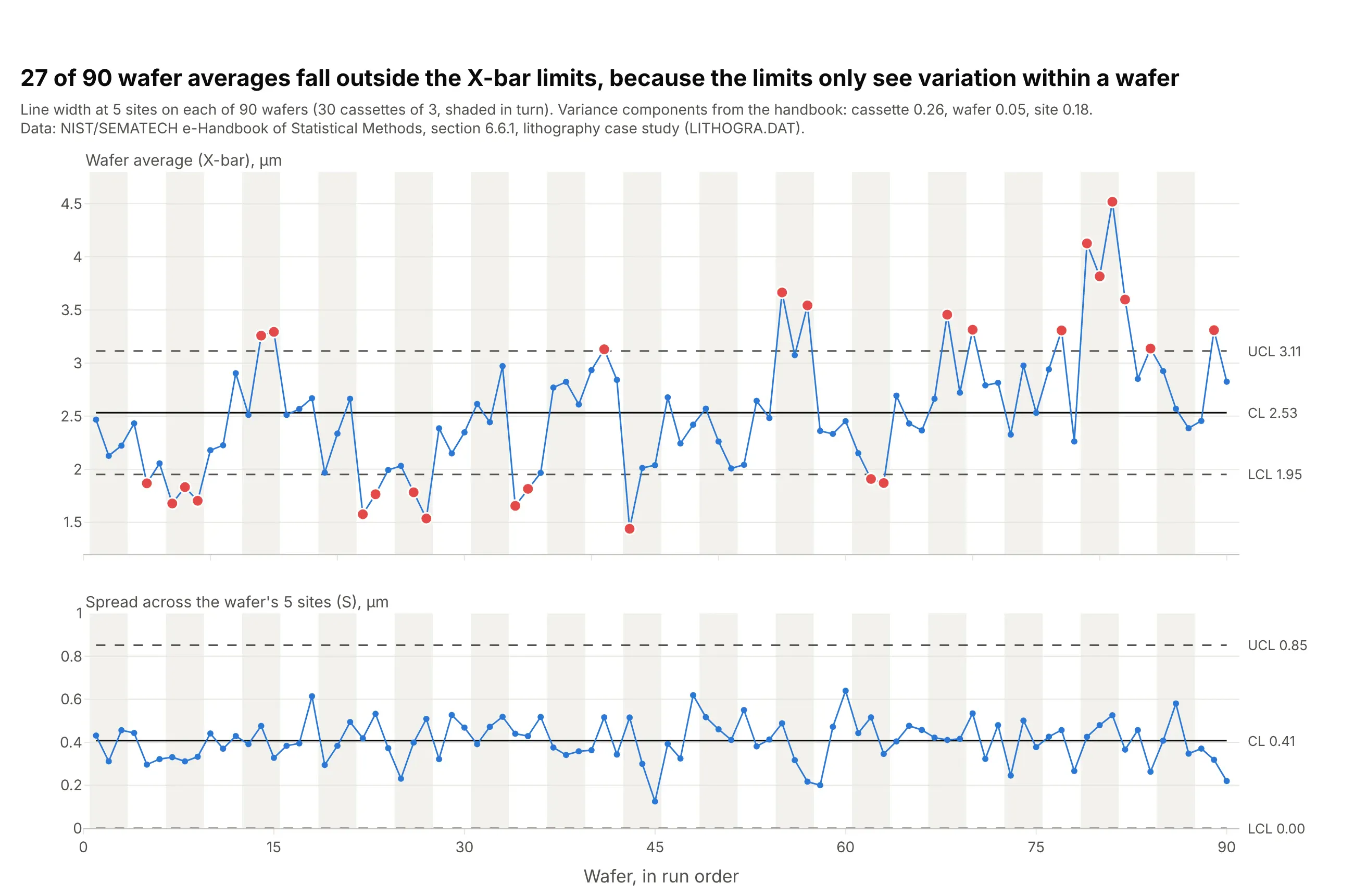
X-bar and S charts of 90 wafers in 30 shaded cassettes: 27 wafer averages in red fall outside narrow X-bar limits of 1.95 and 3.11 µm, rising and falling cassette by cassette, while every wafer's standard deviation stays below its limit of 0.85

27 of 90 wafer averages fall outside the X-bar limits, because the limits only see the spread inside a wafer, and the handbook's variance components show cassette-to-cassette variation (0.26) is larger than site-to-site (0.18). The chart is right that wafers differ by cassette; the lesson is to pick the subgroup on purpose. Data: NIST/SEMATECH e-Handbook of Statistical Methods, 6.6.1, LITHOGRA.DAT.

Tip: shade alternating groups (here cassettes) behind the points, so readers can see points move together.

Get the data from the NIST/SEMATECH e-Handbook lithography case study (itl.nist.gov, datasets/LITHOGRA.DAT,
line width at 5 sites on 3 wafers in each of 30 cassettes) and shape it into a table (columns: cassette, wafer,
site, linewidth_um, run).

Build plotly X-bar and S charts with one subgroup per wafer (n = 5), limits from the average standard deviation
with c4 = 0.94, out-of-limit wafers in red, and alternating cassettes shaded.

2. Great Britain's grid frequency and the August 2019 power cut

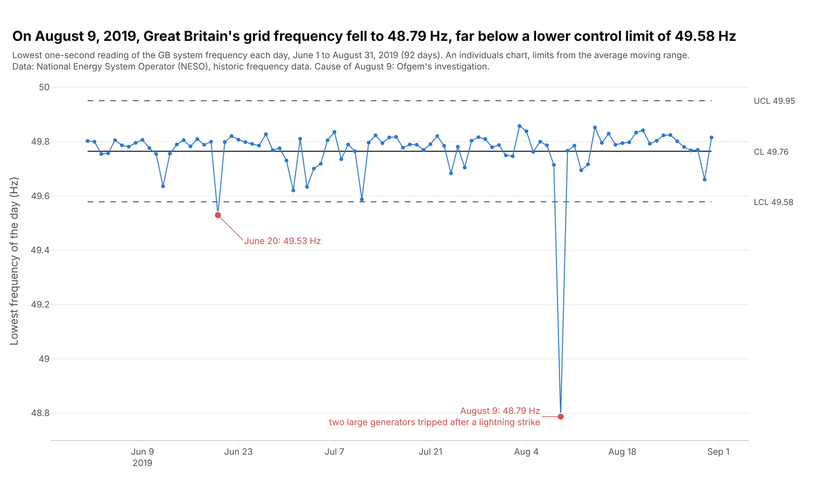
Individuals chart of the lowest grid frequency each day, June to August 2019: days hover near 49.76 Hz between limits of 49.58 and 49.95, June 20 dips just below the lower limit at 49.53 Hz, and August 9 drops to 48.79 Hz, labeled two large generators tripped after a lightning strike

On August 9, 2019, the lowest one-second reading of Great Britain's grid frequency was 48.79 Hz, far below a lower control limit of 49.58 Hz set by the summer's 92 days. The investigation by Ofgem, Great Britain's energy regulator, found two large generators disconnected after a lightning strike, disrupting more than one million consumers. Data: National Energy System Operator (NESO), historic system frequency data.

Tip: reduce millions of one-second readings to one meaningful number per day before charting them as individuals.

Get the data from NESO's historic system frequency data (neso.energy data portal, monthly files for June-August
2019, one reading per second in Hz) and shape it into a table with one row per day (columns: date, min_hz,
max_hz, mean_hz).

Build a plotly individuals control chart of min_hz with limits from the average moving range, out-of-limit days in
red, and each labeled with its date and value.

3. Semmelweis's maternity clinic before and after handwashing

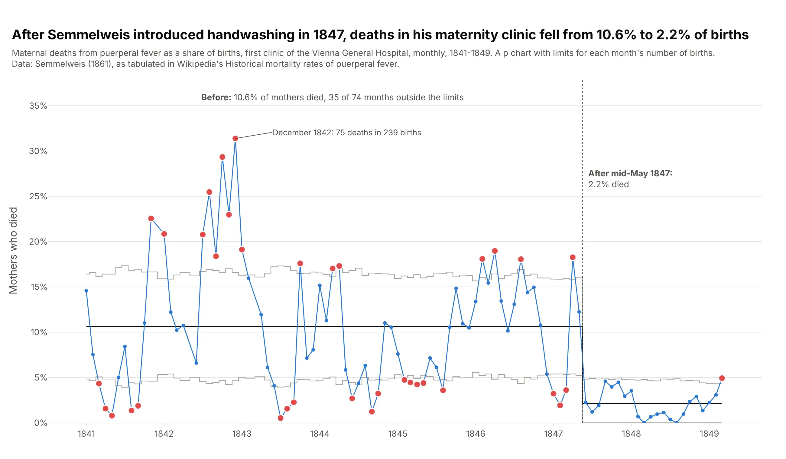
p chart of monthly maternal deaths at Semmelweis's clinic, 1841 to 1849: before mid-May 1847 the share swings between 1% and 31% around 10.6%, with many red months outside step limits near 5% and 16%; after the dotted line in 1847 it stays near 2.2% under a limit near 5%

In Semmelweis's maternity clinic, 10.6% of mothers died of puerperal fever before he made doctors wash their hands in chlorinated lime in mid-May 1847, and 2.2% after. Before the change, 35 of 74 months fell outside their own limits, so deaths were also unpredictable from month to month. Data: Semmelweis (1861), as tabulated in Wikipedia's Historical mortality rates of puerperal fever.

Tip: when the sample size changes every month, draw p chart limits as thin step lines rather than dashes.

Get the data from Wikipedia's "Historical mortality rates of puerperal fever" (Semmelweis 1861, monthly births
and deaths at the first clinic of the Vienna General Hospital, 1841-1849) and shape it into a table (columns:
month, births, deaths, period).

Build a plotly p chart with separate limits before and after June 1847, limits recomputed for each month's births
and drawn as step lines, red months outside them, and a dotted line at mid-May 1847.

4. Nonconformities on printed circuit boards

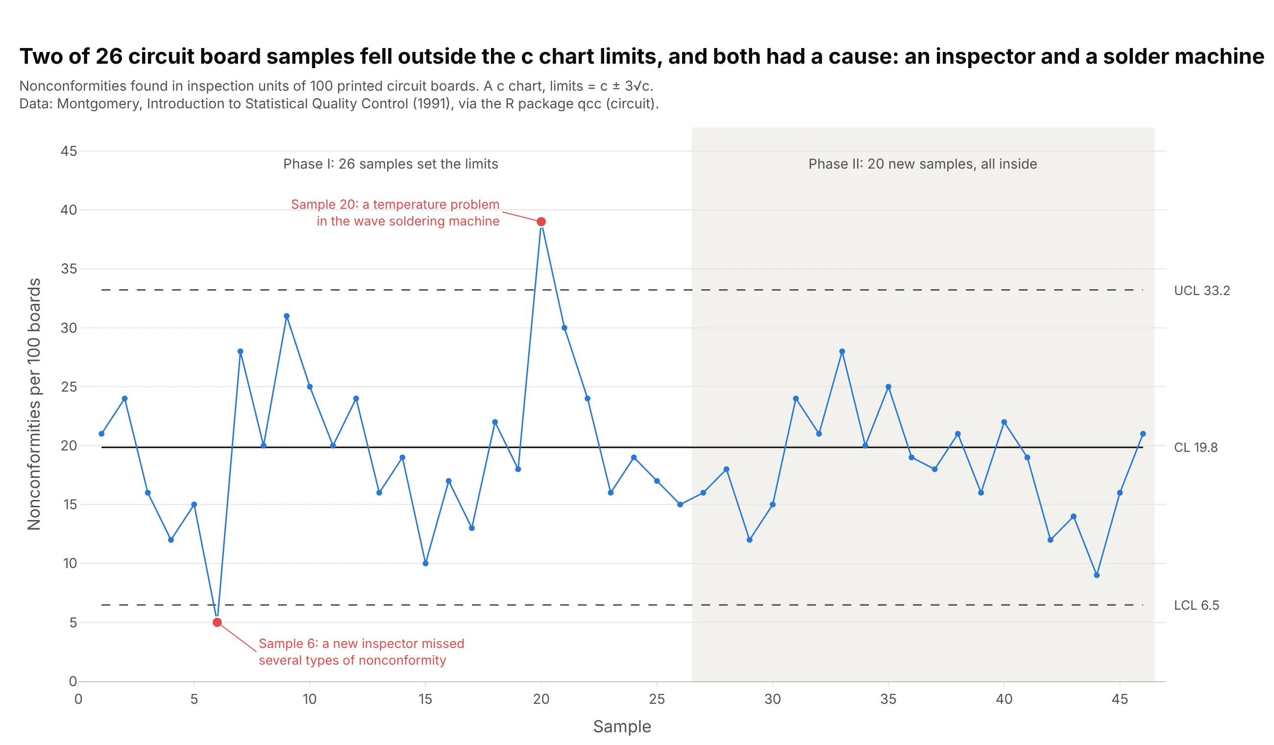
c chart of nonconformities in 46 inspection units of 100 circuit boards: counts vary around 19.8 between limits of 6.5 and 33.2, with sample 6 at 5 labeled a new inspector missed several types of nonconformity and sample 20 at 39 labeled a temperature problem in the wave soldering machine; the 20 phase II samples are all inside

Two of 26 samples of 100 circuit boards fell outside the c chart limits of 6.5 and 33.2 nonconformities, and both had a cause: a new inspector who missed defects and a temperature problem in the wave soldering machine. The 20 samples after the repair stayed inside. Data: Montgomery (1991), via the R package qcc (circuit).

Tip: a low point can be a signal too; here it was an inspection problem, not a better process.

Get the data from the R package qcc's circuit dataset (Montgomery 1991, nonconformities in inspection units of
100 printed circuit boards, 26 trial samples and 20 more) and shape it into a table (columns: sample,
nonconformities, phase).

Build a plotly c chart with limits c +/- 3 x sqrt(c) from the first 26 samples, phase II shaded, and the two
samples outside the limits labeled with their causes.

5. S&P 500 volatility is not a stable process

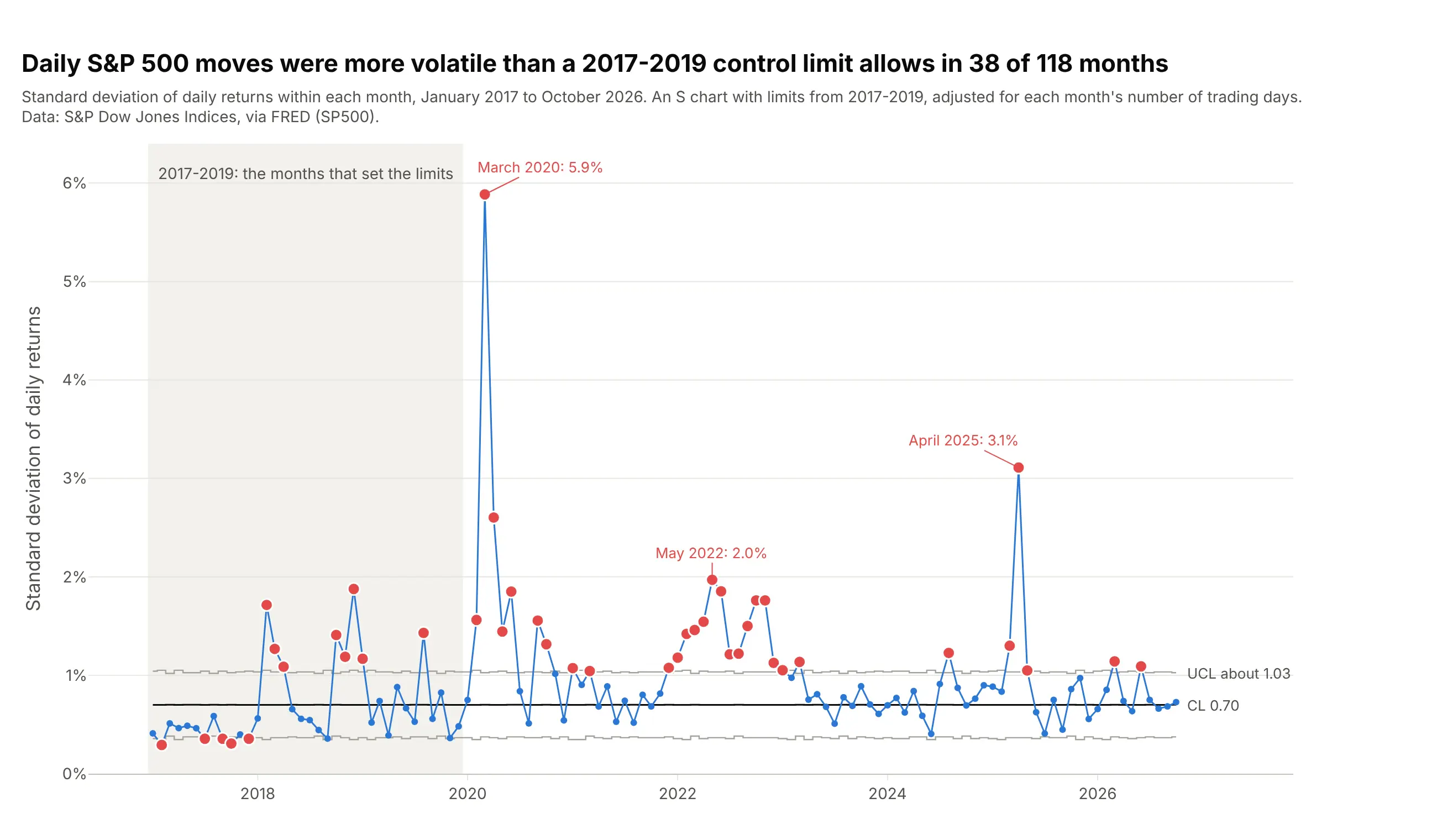
S chart of the monthly standard deviation of daily S&P 500 returns, 2017 to 2026, with limits from the shaded 2017-2019 baseline near 0.70% and 1.03%: 38 months are above the upper limit in red, including March 2020 at 5.9%, May 2022 at 2.0% and April 2025 at 3.1%

With limits from 2017-2019, the day-to-day spread of S&P 500 returns was above the upper limit in 38 of 118 months, including 8 in the baseline itself, and peaked at 5.9% in March 2020. A control chart's verdict here is that market volatility comes in clusters and never settles into statistical control. Data: S&P Dow Jones Indices via FRED (Federal Reserve Economic Data, series SP500).

Tip: if a process is out of control in its own baseline, model it (with a volatility model, for example) instead of charting it against fixed limits.

Get the data from FRED series SP500 (S&P Dow Jones Indices, daily closes) and shape it into a table with one
row per month, 2017-2026 (columns: month, n, sd_pct), where sd_pct is the standard deviation of daily percent
returns.

Build a plotly S chart with limits from 2017-2019 adjusted for each month's number of trading days with c4(n),
the baseline shaded, months above the limit in red and the three largest labeled.

6. Hospital infection rates across 14 health boards

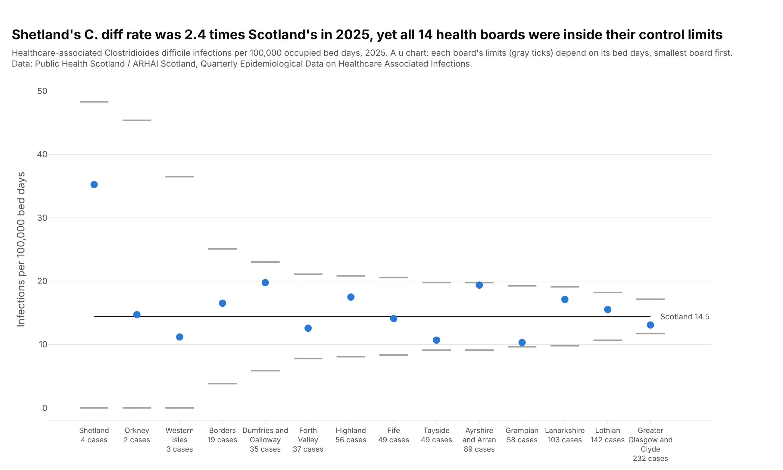
u chart of 2025 C. diff infection rates per 100,000 bed days for Scotland's 14 health boards, sorted by bed days from Shetland to Greater Glasgow and Clyde: gray limit ticks narrow from 0 to 48 for Shetland to 12 to 17 for Glasgow, and every board's dot, including Shetland's at 35.2, is inside its own limits around Scotland's 14.5

Shetland's rate of healthcare-associated C. diff infections was 2.4 times Scotland's in 2025, but that was 4 cases, and its limits run from 0 to 48 per 100,000 bed days, so all 14 boards are inside their limits. A league table would have put Shetland last. Data: Public Health Scotland / ARHAI Scotland, Quarterly Epidemiological Data on Healthcare Associated Infections.

Tip: sort the units by size, so the limits narrow from left to right and readers see why small units swing more.

Get the data from Public Health Scotland's "Quarterly Epidemiological Data on Healthcare Associated Infections"
(opendata.nhs.scot, 2025 quarters, 14 regional NHS boards) and shape it into a table (columns: board, bed_days,
cdi).

Build a plotly u chart of cdi per 100,000 bed days, boards on the x axis sorted by bed days, each board's limits
u +/- 3 x sqrt(u / bed_days) as short horizontal ticks, and the case count under each board name.

Control Charts - A Complete Guide

What is a control chart?

A short history

How control limits are calculated

Sigma, and why the limits sit at 3 sigma

Sample ranges and the average moving range

Fixed limits: phase I and phase II

When the limits do move

Why short-term spread, not the overall standard deviation

Control limits are not specification limits

The rules for out-of-control points

Which control chart to use, and run charts

1. X-bar and R chart

2. X-bar and S chart

3. Individuals and moving range (I-MR) chart

4. p chart and np chart

5. c chart and u chart

6. EWMA and CUSUM charts

7. Run chart

Alternatives to a control chart

How to make a control chart

With AI

With Plotly Studio

Make a control chart in Python or JavaScript

Share it

Dos and don'ts

Checklist

Options to customize

More control chart examples

1. Line width on silicon wafers: the subgroup decides the limits

2. Great Britain's grid frequency and the August 2019 power cut

3. Semmelweis's maternity clinic before and after handwashing

4. Nonconformities on printed circuit boards

5. S&P 500 volatility is not a stable process

6. Hospital infection rates across 14 health boards

FAQ

What is a control chart in simple terms?

How are control limits calculated?

What is the difference between control limits and specification limits?

What is the difference between a run chart and a control chart?

What are the Western Electric rules and the Nelson rules?

Which control chart should I use?

How do I make a control chart in Python?

How many points can a Plotly control chart show?

Can I use a control chart for financial or seasonal data?