Chris Parmer

November 12, 2026

Bland-Altman Plots - A Complete Guide

TL;DR

A Bland-Altman plot compares two ways of measuring the same thing. Each point is one person or sample, with the mean of the two measurements on the x axis and their difference on the y axis, plus a line at the mean difference (the bias) and dashed lines at the 95% limits of agreement, the mean difference plus and minus 1.96 standard deviations (SD).
Bland-Altman plots are also known as Bland-Altman difference plots, mean-difference plots and Tukey mean-difference plots, and they are similar to scatter plots with a line of equality, control charts, which also draw a center line and limits, and the MA plot of gene expression studies (the log ratio M against the mean log intensity A), which is the log ratio version.
They are the standard method comparison plot in clinical measurement: a new blood pressure cuff, lab assay or wearable against the established method, and two readings of the same method to measure repeatability. Engineers and scientists use the same plot for sensors, satellites and models.
Read it in three steps: is the mean difference far from zero, are the limits narrow enough to swap one method for the other, and does the difference change with the size of the measurement (proportional bias, which a regression line or a log ratio version handles).
You can make a Bland-Altman plot with Plotly in Python or JavaScript from a scatter trace and three horizontal lines, with a short helper function that computes the limits.

What is a Bland-Altman plot?

Bland-Altman plots look like this:

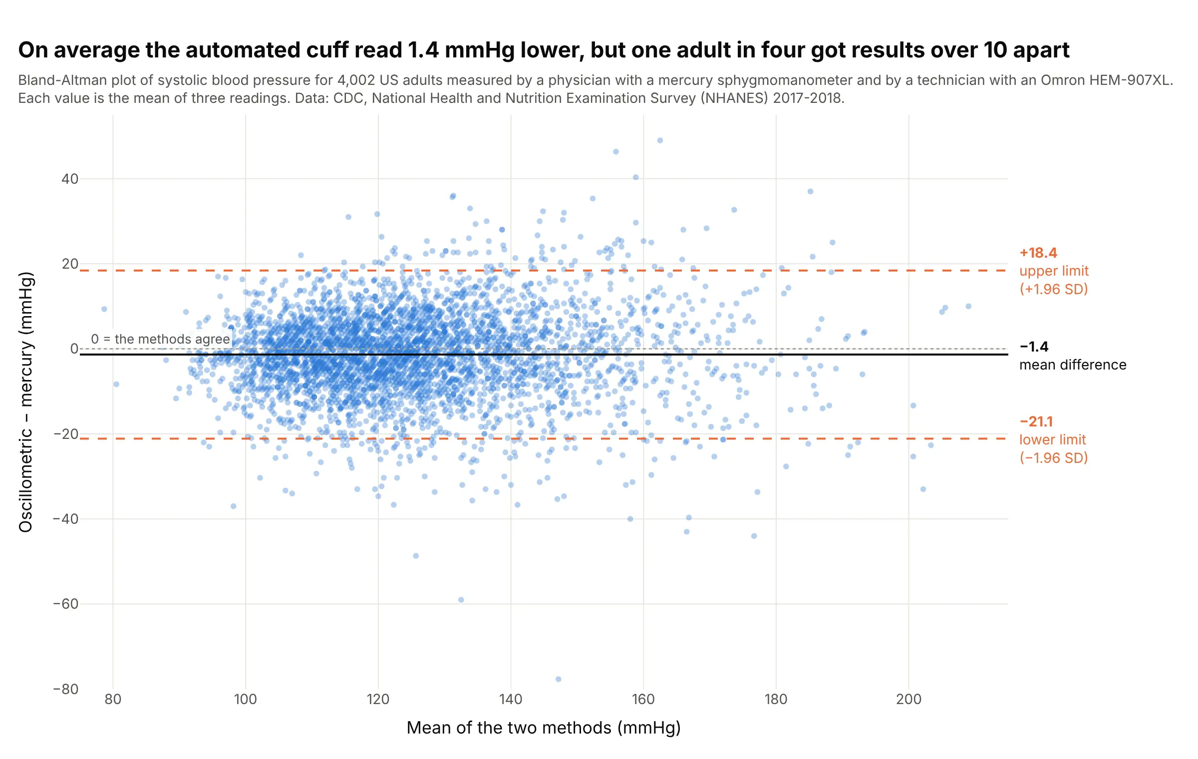
Bland-Altman plot of systolic blood pressure for 4,002 US adults, oscillometric minus mercury against their mean: a cloud of points centered just below zero, a solid line at the mean difference of -1.4 mmHg and dashed lines at the limits of agreement, +18.4 and -21.1 mmHg

Data: US Centers for Disease Control and Prevention (CDC), National Health and Nutrition Examination Survey (NHANES) 2017-2018, blood pressure methodology study: each adult was measured by a physician with a mercury sphygmomanometer and by a technician with an Omron HEM-907XL automated cuff, three readings each, in random order.

How do you read a Bland-Altman plot? In the example above, notice these things:

Each dot is one of 4,002 adults. Its x position is the average of their two blood pressures (the best estimate of the true value), and its height is the automated reading minus the mercury reading, in millimeters of mercury (mmHg).
The solid line is the mean difference, or bias: on average the automated cuff read 1.4 mmHg lower, which is small next to the 125 mmHg average reading.
The dashed lines are the 95% limits of agreement, from 21.1 mmHg below to 18.4 mmHg above. For any one person, the two methods can be expected to differ by that much, and for 26% of these adults they differed by more than 10 mmHg.
The cloud widens at higher pressures: the standard deviation of the differences is 8.4 mmHg for means of 100 to 120 and 14.6 for 160 to 180. So the single pair of limits is a little generous for people with normal blood pressure and too narrow for people with high blood pressure, which regression-based limits (example 2 below) fix.

Whether limits of plus or minus 20 mmHg are acceptable is a clinical judgment, not a statistical one. Bland and Altman's advice is to decide how big a difference would matter before you collect the data.

It's often used for charts like these:

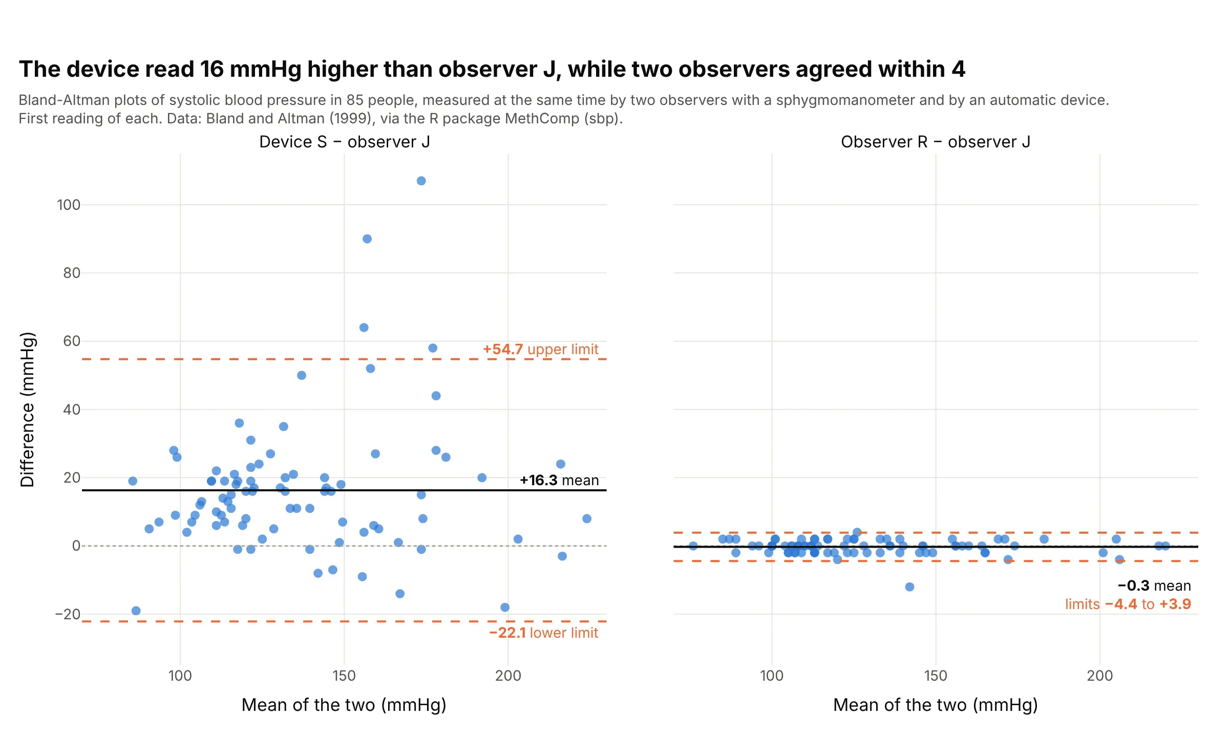
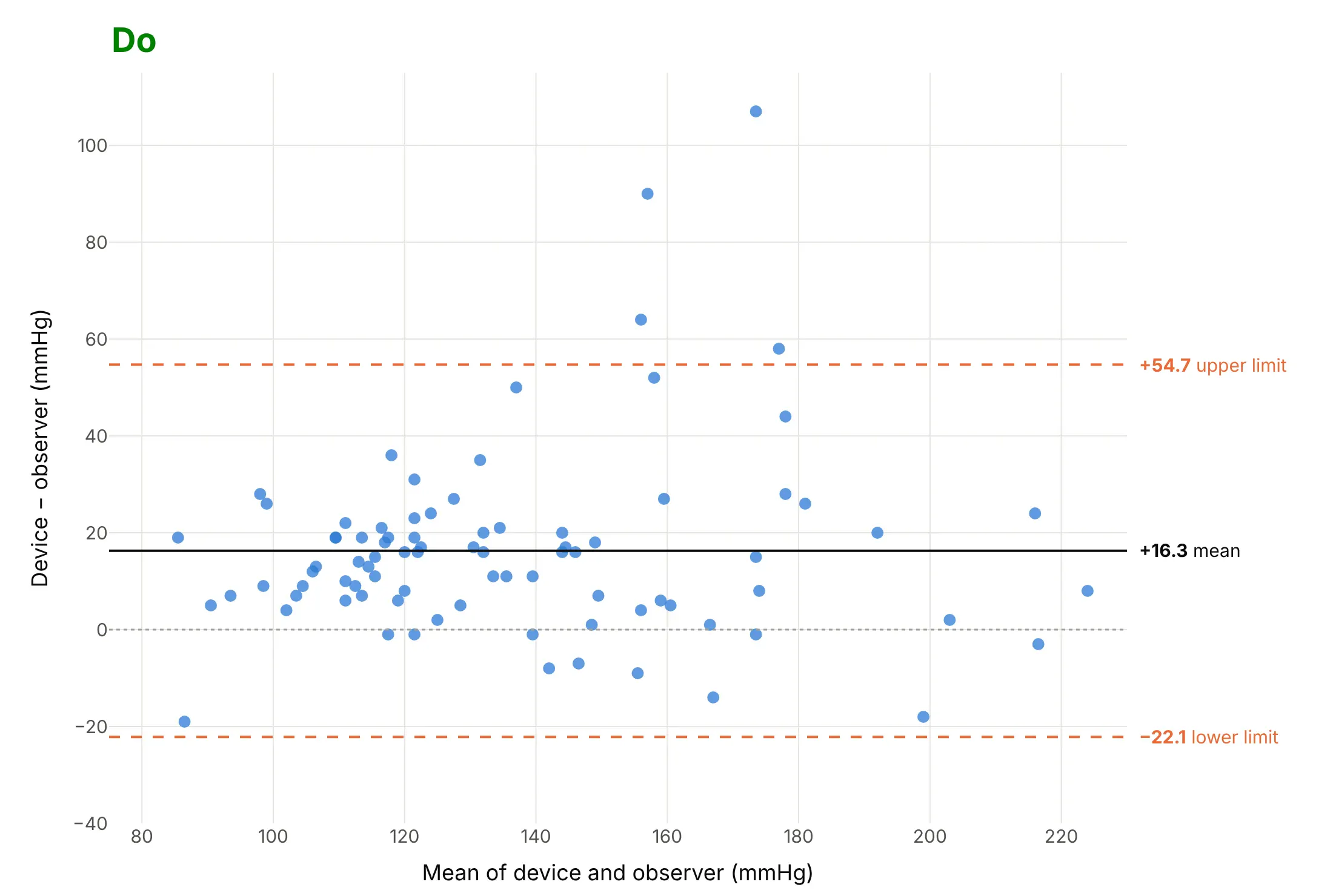
Two Bland-Altman plots of systolic blood pressure in 85 people on the same y scale: an automatic device minus observer J has a mean difference of +16.3 mmHg and limits from -22.1 to +54.7, while observer R minus observer J sits in a thin band with a mean of -0.3 and limits from -4.4 to +3.9

Validating a new device. In Bland and Altman's (1999) textbook data set, an automatic blood pressure device read 16.3 mmHg higher than a trained observer on average, with limits of agreement 77 mmHg wide, while two observers agreed within about 4 mmHg. Data: Bland and Altman (1999), Table 1, as the R package MethComp's sbp data set.

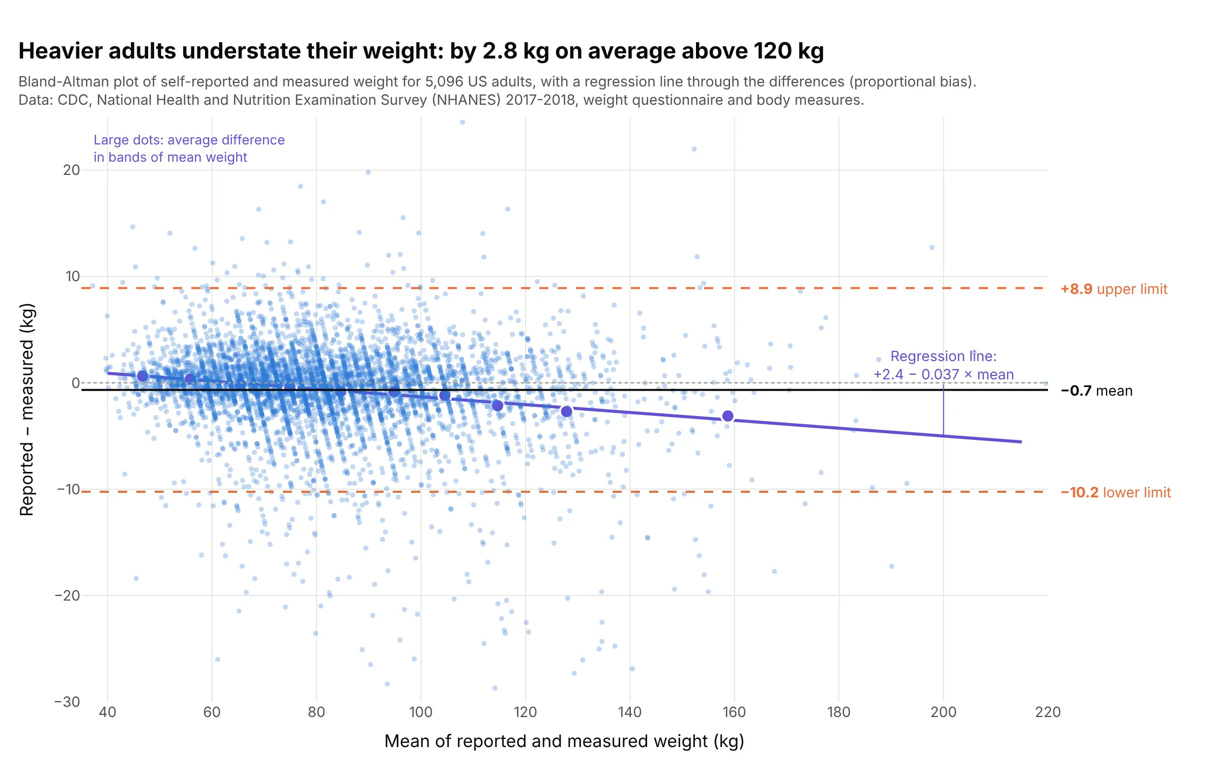
Bland-Altman plot of self-reported minus measured weight for 5,096 US adults: a dense cloud with limits of agreement at +8.9 and -10.2 kg and a purple regression line that slopes down from about +1 kg at 40 kg to -5 kg at 210 kg, with binned averages following it

Checking a survey answer against a measurement. Adults who weigh more understate their weight more: the average error is 0.7 kg, but it runs from +0.4 kg below 60 kg to -2.8 kg above 120 kg, a proportional bias that the purple regression line shows. Data: CDC NHANES 2017-2018, weight questionnaire and body measures.

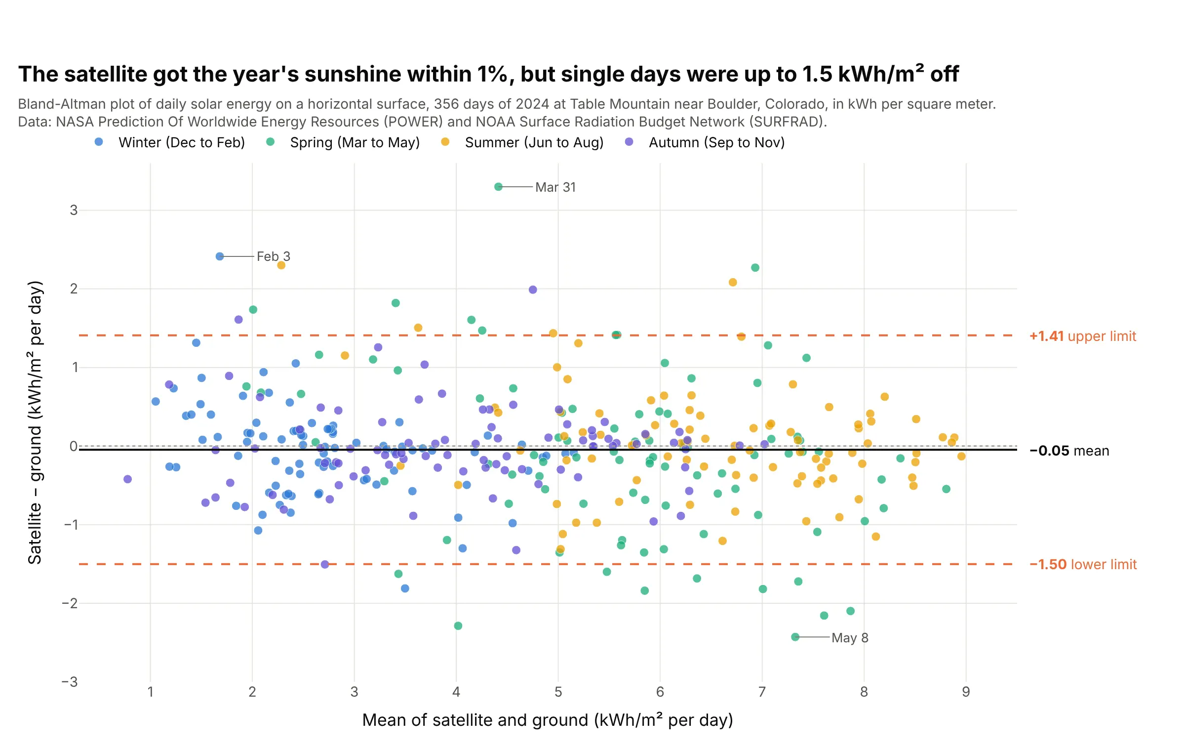
Bland-Altman plot of NASA satellite minus ground-measured daily solar energy at Table Mountain, Colorado, for 356 days of 2024, colored by season: the mean difference is -0.05 kWh per square meter and the limits are -1.50 and +1.41, with March 31 at +3.3 and May 8 at -2.4 labeled

Comparing a model or satellite with a sensor. NASA's satellite-based estimate got the year's solar energy at a Colorado station within 1%, but on a single day it could be 1.5 kWh per square meter off, about 30% of an average day. Data: NASA Prediction Of Worldwide Energy Resources (POWER) and the National Oceanic and Atmospheric Administration (NOAA) Surface Radiation Budget Network (SURFRAD), Table Mountain, 2024.

How the limits of agreement are calculated

The calculation needs nothing more than a mean and a standard deviation. For each person or sample, take the two measurements A and B and compute:

The mean of the two, (A + B) / 2, which goes on the x axis.
The difference, A − B, which goes on the y axis. Always subtract in the same direction, usually new method minus established method, and say which way round it is in the axis title.
The mean of all the differences, d̄. This is the bias: how much A reads above or below B on average.
The standard deviation of the differences, s. This measures how much the differences scatter around the bias.
The 95% limits of agreement, d̄ − 1.96 s and d̄ + 1.96 s. If the differences follow a normal distribution, about 95% of them fall between these two lines.

Here is the main example with the same differences drawn as a histogram on its right edge, so you can see where the limits come from:

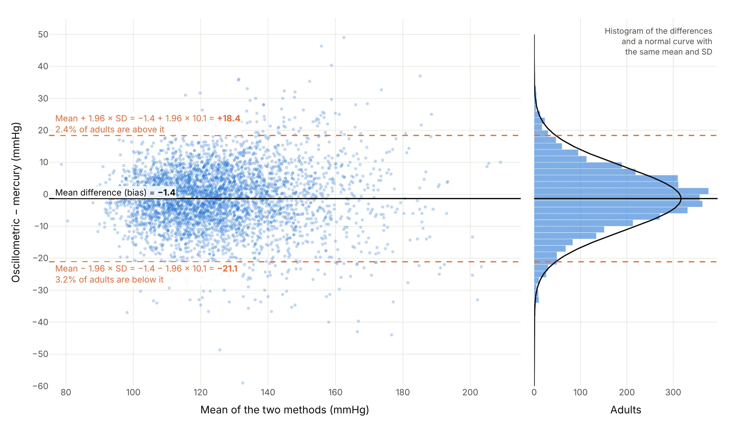
The blood pressure Bland-Altman plot with a histogram of the differences turned sideways on the right and a normal curve with the same mean and SD: the mean difference is -1.4, the upper limit -1.4 + 1.96 x 10.1 = +18.4 with 2.4% of adults above it, and the lower limit -1.4 - 1.96 x 10.1 = -21.1 with 3.2% below it

With a mean difference of -1.4 mmHg and a standard deviation of 10.1 mmHg, the limits are -1.4 ± 1.96 × 10.1, or -21.1 to +18.4 mmHg, and 5.6% of the 4,002 adults fall outside them, close to the 5% the normal distribution predicts. The differences don't need the measurements themselves to be normal, only the differences, which usually are because the person-to-person variation cancels out. A histogram or a Q-Q plot of the differences is the check.

The limits are estimates from a sample, so they have their own uncertainty. Bland and Altman give the standard error of each limit as about √(3s²/n), which for 4,002 people is 0.28 mmHg, but for their original 17 people was 16.3 l/min, wide enough that they reported confidence intervals for the limits too.

Why correlation doesn't measure agreement

Before 1986, most method comparison studies reported a correlation coefficient (r) between the two methods, and many still do. Bland and Altman's paper explains why that answers a different question. Correlation measures whether the points lie along some straight line, not whether they lie along the line of equality, where the two methods give the same number:

A method that always reads 16 mmHg high, or twice as high, can have a correlation close to 1 and still never agree with the other.
Correlation grows with the range of the people you happen to measure. Bland and Altman's peak flow data had r = 0.94 overall, but 0.88 for people below 500 l/min and 0.90 above, even though the two meters disagree by about the same amount in every part of the range, so the lower r in each half reflects the narrower range, not worse agreement.
Two methods designed to measure the same thing will almost always be correlated, so a significant p-value tells you nothing.

The blood pressure example has r = 0.86 and the self-reported weights r = 0.98, and neither number says that the automated cuff can be 20 mmHg away from the mercury reading or that heavy people understate their weight by 3 kg. The Bland-Altman plot says both.

Patterns to look for

Most Bland-Altman plots look like one of these four, all drawn from the data sets in this guide:

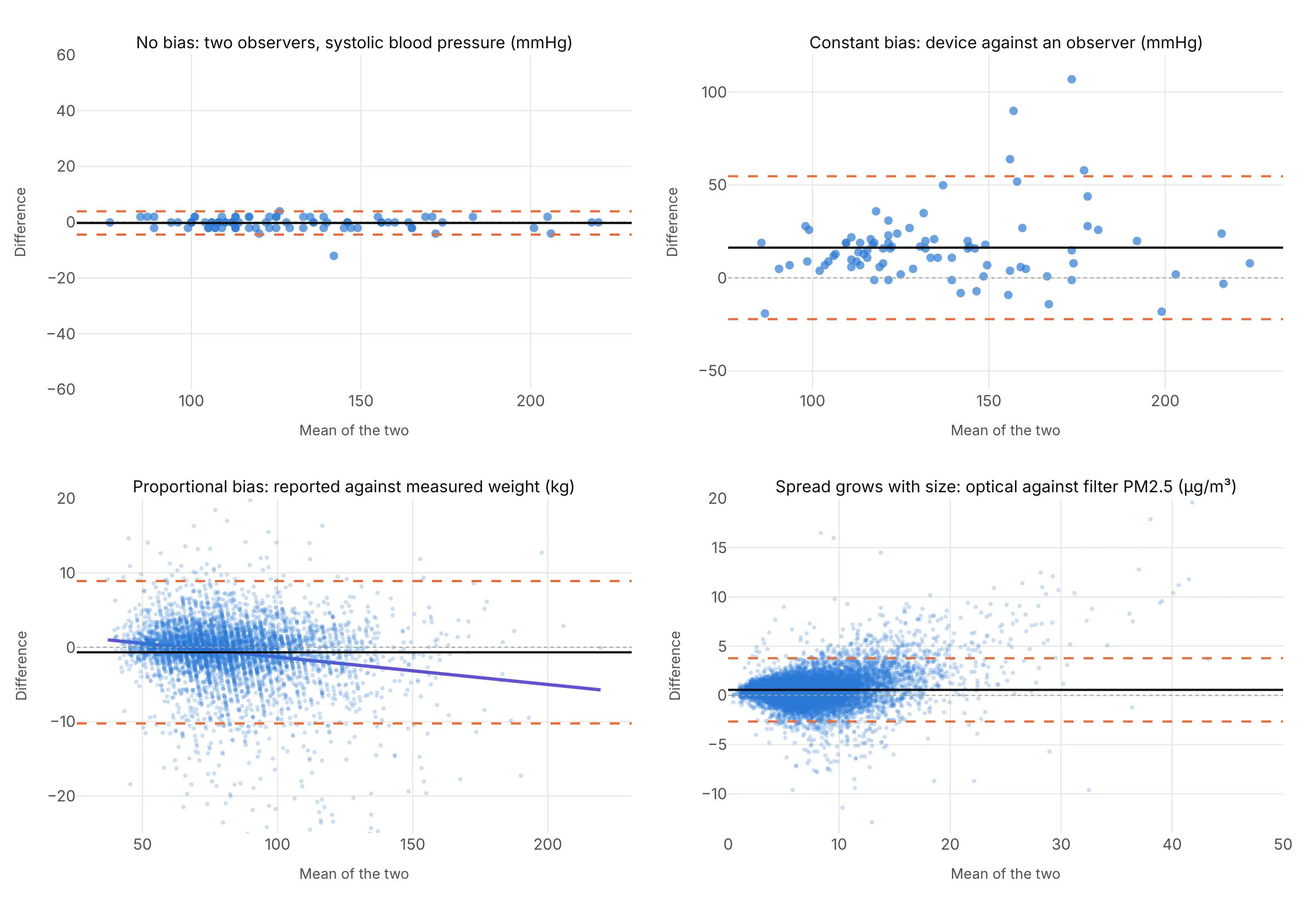
Four Bland-Altman plots: two observers whose differences sit in a thin band around zero (no bias); a device against an observer whose cloud is centered well above zero (constant bias); self-reported weight whose regression line slopes down (proportional bias); and two fine particle monitors whose cloud fans out as the mean grows (spread grows with size)

No bias, narrow limits: the cloud is centered on zero and thin. The methods can be swapped (two trained observers).
Constant bias: the cloud is centered away from zero by the same amount everywhere. You can correct for it by subtracting the mean difference, as long as the limits are narrow enough after that (the device against an observer).
Proportional bias: the cloud tilts, so the difference depends on the size of the measurement. Fit a regression line of difference on mean and report the bias as a line, not a number (self-reported weight).
Spread grows with size: the cloud fans out, so constant limits are too wide at the bottom and too narrow at the top. Plot the ratio of the two methods on a log scale (example 1 below), the percentage difference (example 4), or regression-based limits (example 2). The example here is optical against filter monitors of fine particles (PM2.5, particles under 2.5 micrometers across).

A few points far outside the limits are worth looking up one by one; they are often a transcription error or a failed measurement rather than a property of the method.

A short history

Statisticians Douglas Altman and Martin Bland proposed plotting the difference against the mean in The Statistician in 1983 and brought it to a medical readership in The Lancet in 1986, with peak expiratory flow rate (PEFR) measured on 17 colleagues and family members with a Wright peak flow meter and a mini Wright meter. The Lancet paper had been cited 29,208 times by October 2017, according to Bland, and Nature's 2014 list of the 100 most-cited papers of all time put it at number 29. Their 1999 paper added the variants for repeated measurements, proportional bias and spread that grows with size. Outside medicine the same construction is called a Tukey mean-difference plot, after John Tukey; Wikipedia cites William Cleveland's Visualizing Data (1993) for the name. This is the original example, redrawn from the paper's Table 1:

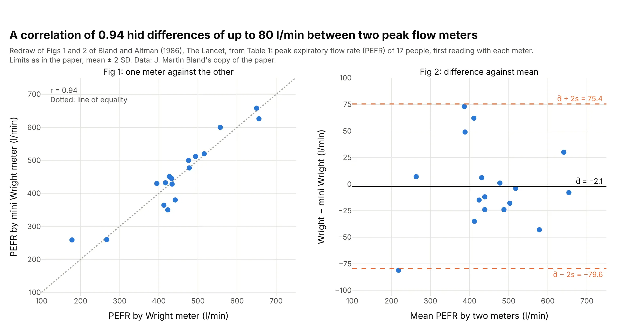
Redraw of Figs 1 and 2 of Bland and Altman (1986): on the left, 17 peak flow readings by the mini Wright meter against the Wright meter lie close to the line of equality with r = 0.94; on the right, the same data as differences against means, with the mean difference at -2.1 and limits at +75.4 and -79.6 l/min

On the scatter plot the two meters look interchangeable. On the difference plot, the mini meter could read up to 80 l/min above or 75 l/min below the Wright meter, which the authors judged unacceptable for clinical use. The paper drew its limits at two standard deviations; 1.96 gives -78.1 to +73.9 l/min.

Alternatives to a Bland-Altman plot

Here's the same blood pressure data drawn six ways. Some are better for the question, some worse, some just different:

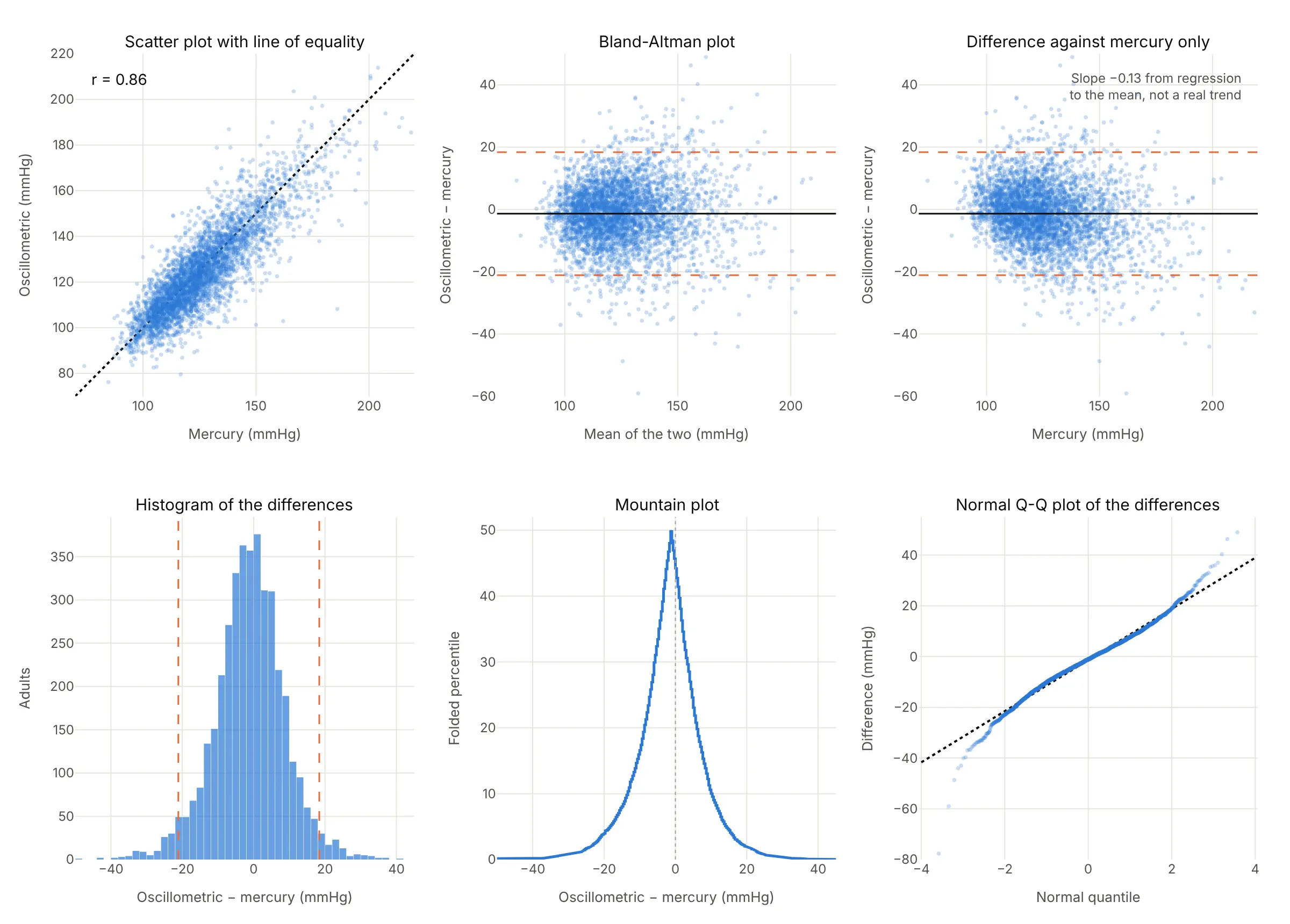
The 4,002 pairs of blood pressure readings drawn six ways: a scatter plot of oscillometric against mercury with a dotted line of equality and r = 0.86; the Bland-Altman plot; the difference plotted against the mercury reading alone, which tilts down with a slope of -0.13; a histogram of the differences with the limits marked; a mountain plot, a peaked curve centered just below zero; and a normal Q-Q plot of the differences that is close to straight

Scatter plot with a line of equality (worse for agreement, works too as a first look). Bland and Altman recommend drawing it first, but the points crowd near the line and a 20 mmHg disagreement is hard to see at this scale. Leave out the regression line and the correlation.
Difference against one method (worse). Plotting against the established method instead of the mean builds in a false trend, because the reference's own measurement error appears on both axes. Here it tilts with a slope of -0.13 though there's no real trend; Bland explains this statistical artifact in detail.
Histogram of the differences (works too, as a companion). It shows the bias and the spread and checks the normality the limits assume, but it can't show whether the difference depends on the size of the measurement.
Mountain plot (different). A folded empirical cumulative distribution function (ECDF) of the differences: the peak sits at the median difference and the width at any height reads as a percentile range. It has the same blind spot as the histogram.
Q-Q plot of the differences (different). It checks whether the differences are normal, which the 1.96 rule assumes. Here they are close to straight, with heavier tails beyond about 2 standard deviations.

Regression methods built for two noisy methods, such as Deming and Passing-Bablok regression, estimate a slope and an intercept between the methods. They answer whether there's a systematic difference, not how far apart one person's two results can be.

How to make a Bland-Altman plot

With AI

ChatGPT, Claude Code, GitHub Copilot, Cursor and other AI tools are excellent at writing Plotly code. Name Plotly in the prompt, and say which method is subtracted from which and how to draw the limits:

Make a plotly Bland-Altman plot from bp.csv (columns: id, mercury, oscillometric, systolic blood pressure in mmHg).

- x = (oscillometric + mercury) / 2, y = oscillometric - mercury, go.Scattergl markers at 0.35 opacity.
- A solid line at the mean difference, dashed lines at mean ± 1.96 × SD of the differences, a dotted
  line at 0, each labeled with its value in the right margin.
- Fit a regression line of difference on mean and print its slope and p-value, to check for proportional bias.
- Axis titles "Mean of the two methods (mmHg)" and "Oscillometric − mercury (mmHg)". A title that states the
  bias and the limits.
- Check: print how many points fall outside the limits (it should be close to 5%).

With Plotly Studio

Plotly Studio is a desktop app where you point an AI at a dataset and it builds charts and a Dash app around your questions. Ask for a Bland-Altman plot the same way:

Show a Bland-Altman plot of serum against plasma glucose, with a toggle between differences in mg/dL and the ratio on a log scale, the 95% limits of agreement labeled, and a dropdown to filter by age group.

Make a Bland-Altman plot in Python or JavaScript

This is the code AI tools write under the hood. In Python, a Bland-Altman plot is a scatter trace of means and differences plus three horizontal lines, so a short helper function covers every example in this guide:

import numpy as np
import plotly.graph_objects as go


def bland_altman(a, b, names=("A", "B"), units=""):
    """Bland-Altman plot of two methods measuring the same things: a - b against (a + b) / 2."""
    a, b = np.asarray(a, float), np.asarray(b, float)
    mean, diff = (a + b) / 2, a - b
    bias, sd = diff.mean(), diff.std(ddof=1)
    lo, hi = bias - 1.96 * sd, bias + 1.96 * sd

    fig = go.Figure(go.Scatter(x=mean, y=diff, mode="markers", marker=dict(size=9, opacity=0.7)))
    fig.add_hline(y=0, line=dict(color="gray", dash="dot"))
    fig.add_hline(y=bias, line=dict(color="black"), annotation_text=f"Mean {bias:+.1f}")
    for v, label in [(hi, "+1.96 SD"), (lo, "−1.96 SD")]:
        fig.add_hline(y=v, line=dict(color="#eb6834", dash="dash"), annotation_text=f"{label}: {v:+.1f}")
    fig.update_layout(xaxis_title=f"Mean of {names[0]} and {names[1]} {units}",
                      yaxis_title=f"{names[0]} − {names[1]} {units}", showlegend=False)
    return fig


# Bland and Altman (1986), Table 1: peak flow (l/min) by a Wright meter and a mini Wright meter
wright = [494, 395, 516, 434, 476, 557, 413, 442, 650, 433, 417, 656, 267, 478, 178, 423, 427]
mini = [512, 430, 520, 428, 500, 600, 364, 380, 658, 445, 432, 626, 260, 477, 259, 350, 451]
fig = bland_altman(wright, mini, names=("Wright", "mini Wright"), units="(l/min)")
fig.show()

For the ratio version, pass np.log(a) and np.log(b), then report np.exp of the bias and limits as ratios, or plot a / b on a log y axis as in example 1 below. For thousands of points, switch go.Scatter to go.Scattergl. statsmodels has a matplotlib version, sm.graphics.mean_diff_plot, whose documentation calls it "Tukey's Mean Difference Plot (also known as a Bland-Altman plot)"; the Plotly version adds hover labels on every point, zoom and a chart that drops into a Dash app.

In JavaScript, plotly.js draws the same chart from a scatter trace and three line shapes:

<div id="chart"></div>
<script src="https://cdn.plot.ly/plotly-4.1.1.min.js"></script>
<script>
  // Bland and Altman (1986), Table 1: peak flow (l/min) by a Wright meter and a mini Wright meter
  const wright = [494, 395, 516, 434, 476, 557, 413, 442, 650, 433, 417, 656, 267, 478, 178, 423, 427];
  const mini = [512, 430, 520, 428, 500, 600, 364, 380, 658, 445, 432, 626, 260, 477, 259, 350, 451];

  const mean = wright.map((w, i) => (w + mini[i]) / 2);
  const diff = wright.map((w, i) => w - mini[i]);
  const bias = diff.reduce((s, d) => s + d, 0) / diff.length;
  const sd = Math.sqrt(diff.reduce((s, d) => s + (d - bias) ** 2, 0) / (diff.length - 1));
  const [lo, hi] = [bias - 1.96 * sd, bias + 1.96 * sd];

  const line = (y, color, dash) => ({type: "line", xref: "paper", x0: 0, x1: 1, y0: y, y1: y,
                                     line: {color: color, dash: dash}});
  const label = (y, text) => ({xref: "paper", x: 1, y: y, text: text, showarrow: false,
                               xanchor: "right", yanchor: "bottom"});

  Plotly.newPlot("chart", [{x: mean, y: diff, mode: "markers", marker: {size: 9}}], {
    width: 800, height: 520, showlegend: false,
    shapes: [line(0, "gray", "dot"), line(bias, "black", "solid"), line(lo, "#eb6834", "dash"), line(hi, "#eb6834", "dash")],
    annotations: [label(bias, `Mean ${bias.toFixed(1)}`), label(hi, `+1.96 SD: ${hi.toFixed(1)}`),
                  label(lo, `−1.96 SD: ${lo.toFixed(1)}`)],
    xaxis: {title: {text: "Mean of the two meters (l/min)"}},
    yaxis: {title: {text: "Wright − mini Wright (l/min)"}}
  });
</script>

Share it

Every Plotly chart has a Share chart button (the cloud icon in its toolbar) that uploads it to Plotly Cloud and gives you a link. Only you can see it until you change its visibility.

For a live app, put the chart in a Dash app and publish it with the Plotly Cloud command-line interface (CLI). Coding agents can run these commands for you:

pip install "dash[cloud]"
plotly user login
plotly app publish

If your data has to stay in your own cloud or data center, publish to Dash Enterprise instead.

Dos and don'ts

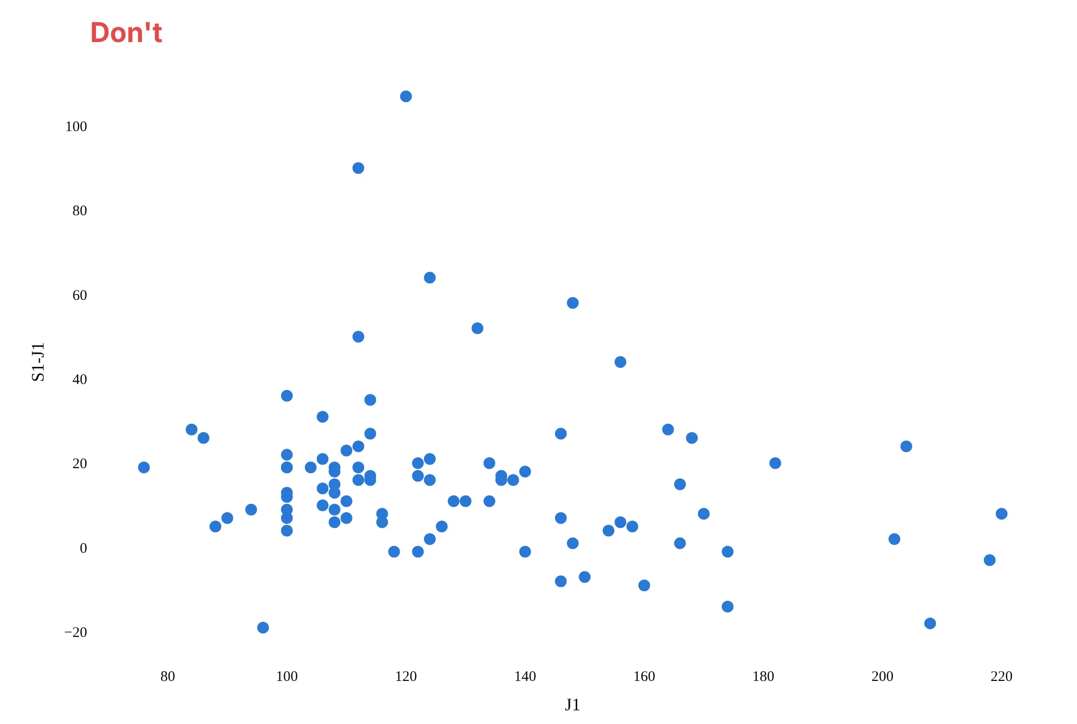
A Bland-Altman plot is only useful if the reader can see the bias and the limits and knows which way the subtraction goes. Here are the device and observer blood pressures both ways, in the same color.

Don't plot the difference against one of the methods, which builds in a false downward trend, leave out the mean difference and the limits, use raw column names like S1-J1 as axis titles, or use a default serif font:

The device-minus-observer differences plotted against observer J's reading, with no mean or limit lines, axis titles J1 and S1-J1, large markers and a serif font

Do put the mean of the two methods on x, draw the mean difference as a solid line and the limits as dashed lines labeled with their values, add a dotted line at zero, and write the axis titles in words with the direction of the subtraction and the units:

The same 85 people with the mean of device and observer on x, the difference on y, a solid line labeled +16.3 mean, dashed lines labeled +54.7 upper limit and -22.1 lower limit, and a dotted line at zero

Checklist

Say which method is subtracted from which in the y axis title ("Device − observer (mmHg)").
Label the mean difference and both limits with their values, so nobody has to read them off the axis.
Keep a dotted line at zero, so the bias reads as the gap between two lines.
Decide before you look what difference would be clinically or practically acceptable, and draw it if it helps.
Use transparent markers or go.Scattergl for thousands of points, and add a histogram of the differences when the audience will ask about normality.
Switch to the ratio (log) version when the spread grows with the size of the measurement.

Don't

Report the correlation coefficient as evidence of agreement.
Put one method alone on the x axis, unless it is a true reference with negligible error.
Average repeated readings and then compute the limits without correcting for it; averaging shrinks the standard deviation of the differences (Bland and Altman 1986 give the correction).
Read the limits from fewer than about 30 pairs without their confidence intervals.

Options to customize

A Bland-Altman plot in Plotly is a scatter trace plus reference lines, so these are the options that matter most. The full lists are in the scatter trace reference, the scattergl trace reference and the shapes reference.

fig.add_hline(y=..., line_dash=..., annotation_text=...): the mean difference, the limits and the zero line, each with a label, in one call per line.
go.Scattergl: WebGL markers for thousands to millions of pairs.
marker.opacity, marker.size: 0.2 to 0.4 opacity and 4 to 6 px for big samples, so the density shows and rounded values don't stack into solid stripes.
customdata and hovertemplate: both original measurements and the sample ID in the hover, so an outlier can be traced to a record.
yaxis.type="log" with tickvals and ticktext: the ratio version, with ticks labeled as ratios (0.9, 1, 1.1) rather than logs.
go.Scatter(mode="lines") for sloped or curved lines: a regression line for proportional bias, or regression-based limits that widen with the mean.
marker.color with a colorscale and colorbar, or one trace per group: color by a third variable (season, sun angle, year) to see what drives the differences.
make_subplots(shared_yaxes=True): two comparisons side by side on the same scale, such as a device against an observer and two observers against each other.
add_hrect: a shaded band for the limits or for a clinically acceptable difference.
Marginal histogram with make_subplots(column_widths=[0.75, 0.25]) and go.Histogram(y=diff): the distribution of the differences next to the plot, as in the marginal plot guide.

More Bland-Altman plot examples

Six more Bland-Altman plots built from real public data, each with its source, the technique that makes it work and a prompt to rebuild it.

1. Serum against plasma glucose, the ratio version

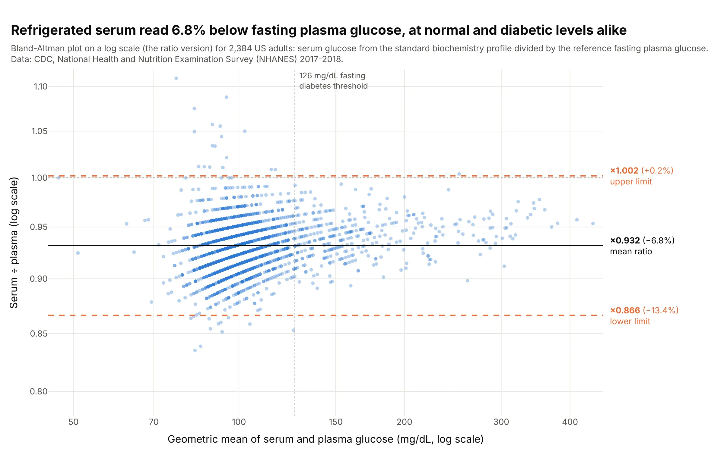
Bland-Altman plot on log scales of refrigerated serum glucose divided by fasting plasma glucose for 2,384 US adults: points centered on a mean ratio of 0.932 (-6.8%), with limits of agreement at 0.866 (-13.4%) and 1.002 (+0.2%), and a dotted vertical line at the 126 mg/dL diabetes threshold

Glucose measured in refrigerated serum read 6.8% below the reference fasting plasma glucose, with 95% of ratios between 0.87 and 1.00. Because the gap grows with the glucose level, the ratio version gives one pair of limits for the whole range: 84 of the 401 adults at or above 126 mg/dL by plasma fell below it by serum. Data: CDC NHANES 2017-2018, standard biochemistry profile and fasting plasma glucose.

Tip: plot the ratio on a log axis and label the ticks as ratios and the limits as percentages, so readers don't have to take antilogs.

Get the data from CDC NHANES 2017-2018 files GLU_J (LBXGLU, fasting plasma glucose, mg/dL), BIOPRO_J
(LBXSGL, refrigerated serum glucose, mg/dL) and DEMO_J (RIDAGEYR), adults 20 and over with both
(columns: seqn, age, plasma, serum).

Build a plotly Bland-Altman plot of the ratio: x = sqrt(serum × plasma) on a log axis, y = serum / plasma
on a log axis with ticks 0.85 to 1.10, the geometric mean ratio and exp(mean ± 1.96 SD of log ratio) as
lines labeled as ratios and percentages, and a vertical line at 126 mg/dL.

2. Optical against filter monitors for fine particles, with regression-based limits

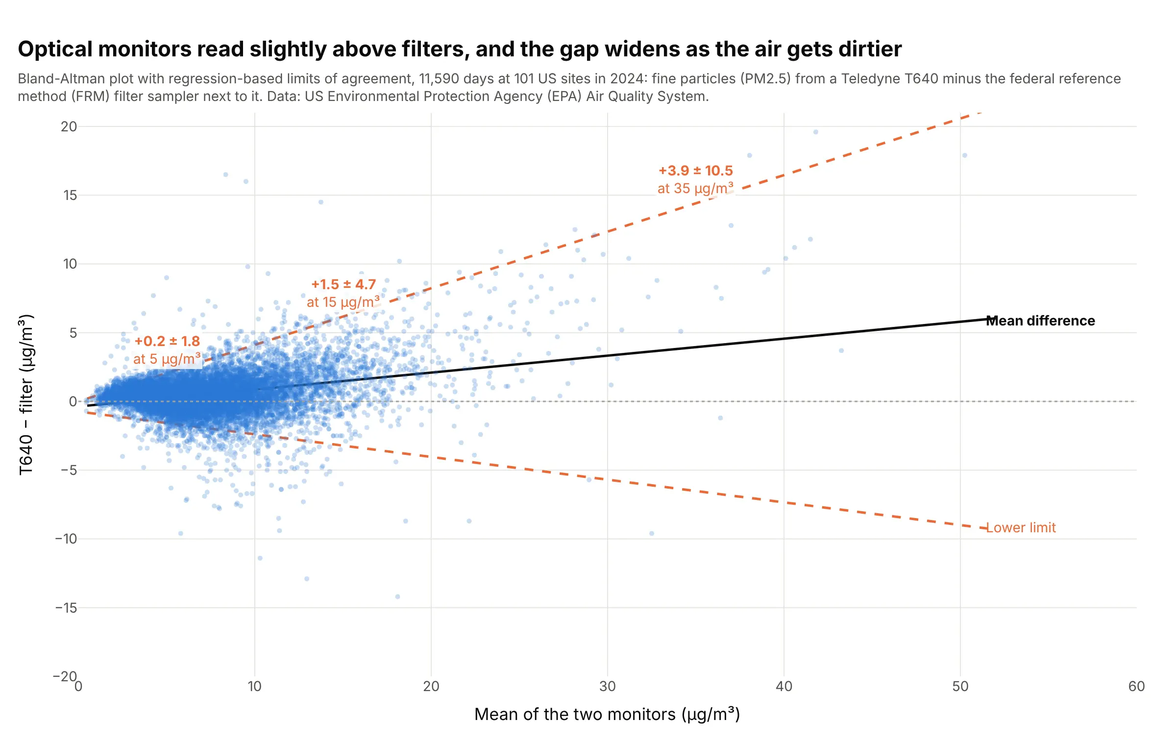
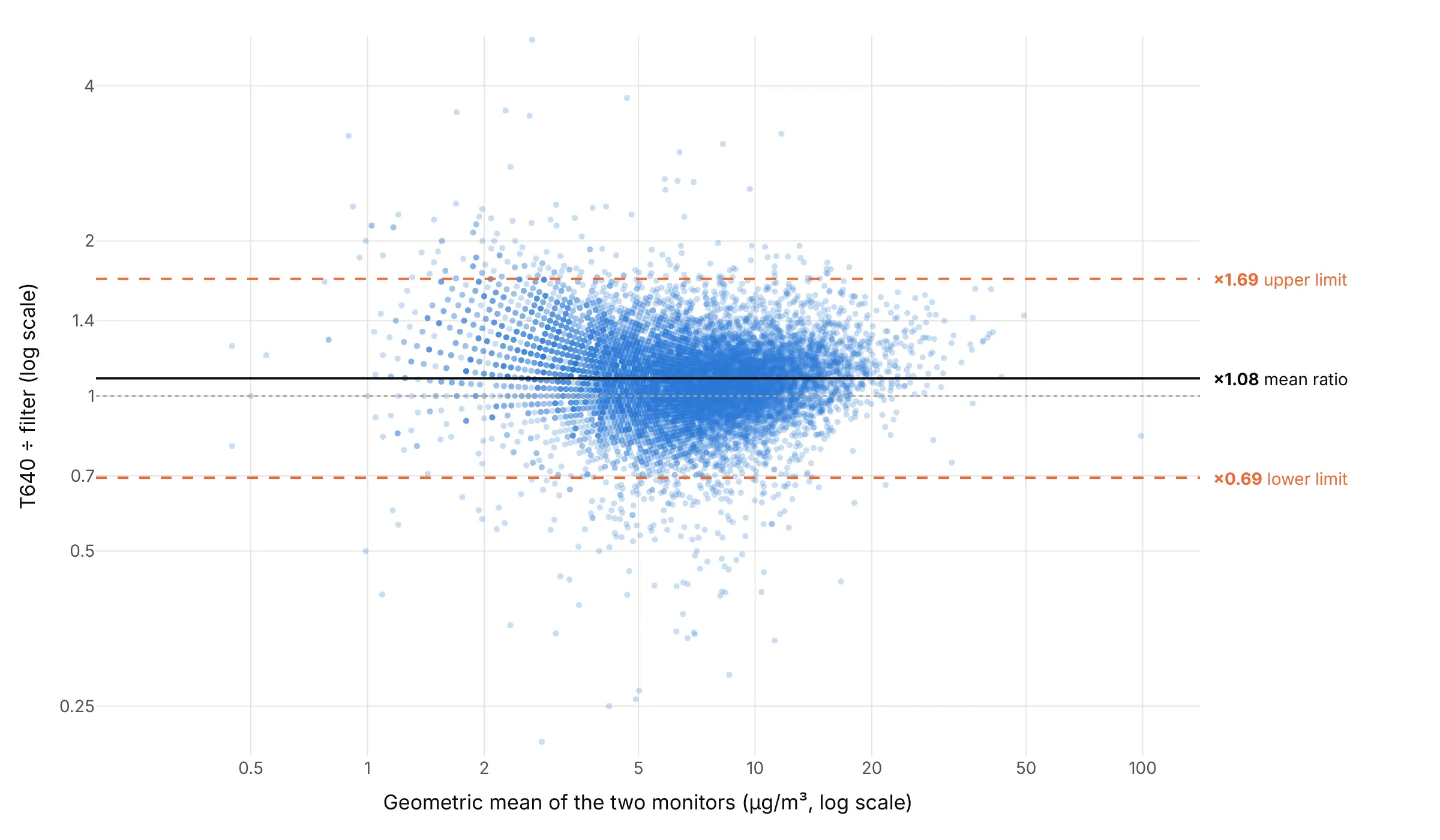
Bland-Altman plot of 11,590 days at 101 US air monitoring sites: Teledyne T640 minus filter PM2.5 against their mean, a mean difference line rising from about 0 to +6 micrograms per cubic meter and dashed limits that fan out, labeled +0.2 ± 1.8 at 5, +1.5 ± 4.7 at 15 and +3.9 ± 10.5 at 35

At 101 US sites where a Teledyne T640 optical monitor ran next to a federal reference method (FRM) filter sampler in 2024, the difference in fine particles (PM2.5, particles under 2.5 micrometers across) grows from +0.2 ± 1.8 micrograms per cubic meter on clean days to +3.9 ± 10.5 at 35. Regression-based limits (Bland and Altman 1999) follow that fan where flat lines would not. Data: US Environmental Protection Agency (EPA) Air Quality System daily PM2.5 files, 2024.

Tip: regress the absolute residuals on the mean and draw the limits as the fitted line ± 1.96 × √(π/2) times that fit.

Get the data from the EPA Air Quality System pre-generated daily file daily_88101_2024.zip, keeping
method code 145 (filter) and 636 (Teledyne T640) at the same site and date, standard "PM25 24-hour 2012"
(columns: site, date, state, frm, t640).

Build a plotly Bland-Altman plot with go.Scattergl at 0.25 opacity, a regression line of t640 - frm on the
mean, and limits that widen with the mean (Bland and Altman 1999, section 3.2), labeled at 5, 15 and 35 µg/m³.

Another way to see it: the same days as a ratio on log scales give one pair of horizontal limits, from 0.69 to 1.69 times the filter value, around a mean ratio of 1.08:

The same 11,590 site-days as T640 divided by filter on a log y axis against the geometric mean on a log x axis: points around a mean ratio of 1.08 with limits at 0.69 and 1.69

3. Repeatability: the same method twice

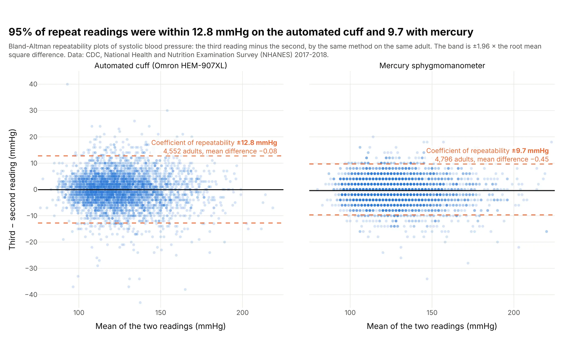
Two Bland-Altman repeatability plots of the third minus the second systolic reading: the automated cuff with a coefficient of repeatability of ±12.8 mmHg for 4,552 adults, and the mercury sphygmomanometer with ±9.7 mmHg for 4,796 adults, its points stacked on even numbers

Plotting a method against itself gives the coefficient of repeatability: in 95% of adults, two back-to-back readings were within 12.8 mmHg on the automated cuff and 9.7 mmHg with mercury. This limits how well the two methods can ever agree with each other, which is why the 1986 paper covers repeatability next to agreement. Data: CDC NHANES 2017-2018, blood pressure readings 2 and 3 by each method.

Tip: for repeatability, compute the limits as ±1.96 × √(mean of the squared differences), since the true mean difference is zero.

Get the data from CDC NHANES 2017-2018 files BPXO_J (BPXOSY2, BPXOSY3) and BPX_J (BPXSY2, BPXSY3),
adults 20 and over from DEMO_J (columns: seqn, osc2, osc3, aus2, aus3).

Build two plotly Bland-Altman plots side by side with shared y: third minus second reading against their
mean for each method, a shaded band at ± 1.96 × sqrt(mean(d²)), and the coefficient of repeatability
in each panel.

4. A solar instrument against the sum of two others, in percent

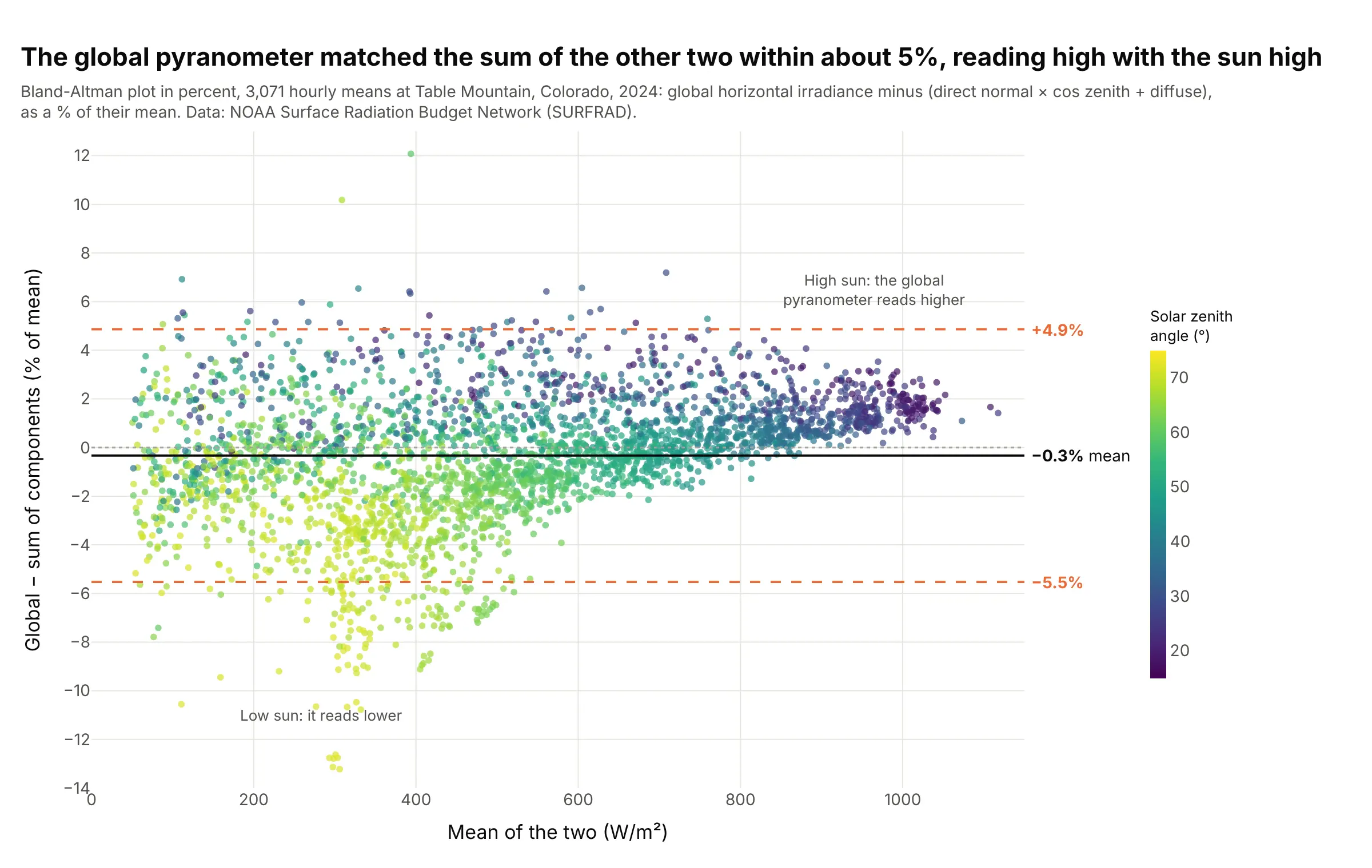
Bland-Altman plot in percent of 3,071 hourly means at Table Mountain, Colorado, in 2024: global pyranometer minus the sum of direct and diffuse components against their mean, colored by solar zenith angle, with high-sun points above zero, low-sun points below, a mean of -0.3% and limits at +4.9% and -5.5%

Radiation networks check their instruments by comparing an unshaded pyranometer with the sum of a direct beam reading and a shaded diffuse one. At Table Mountain in 2024, 95% of hours agreed within -5.5% to +4.9%, and coloring by sun angle shows why the spread exists: the pyranometer reads 2.3% high with the sun near overhead and 4.6% low with it 70 to 75 degrees from overhead. Data: NOAA SURFRAD, Table Mountain, 1-minute data, 2024.

Tip: when the difference grows with the measurement, divide it by the mean and plot it in percent.

Get the data from NOAA SURFRAD Table Mountain (tbl) 2024 daily files of 1-minute data (columns: time,
zen, dw_solar, direct_n, diffuse, and their quality flags), keeping minutes with flags 0 and zenith
below 75 degrees, averaged by hour.

Build a plotly Bland-Altman plot of 100 × (dw_solar - sum) / mean, where sum = direct_n × cos(zen) +
diffuse, colored by zenith angle with a Viridis colorbar, with the mean and limits labeled in percent.

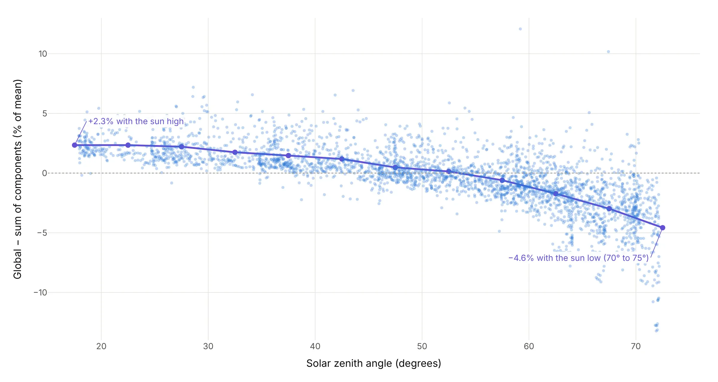
Another way to see it: plotting the same percent differences against the sun's zenith angle instead of the mean turns the cloud into a clear curve, from +2.3% with the sun high to -4.6% with it low:

The same hourly percent differences plotted against solar zenith angle from 15 to 75 degrees, with averages in 5-degree bins falling from +2.3% to -4.6%

5. GDP against GDI, two measures of the US economy

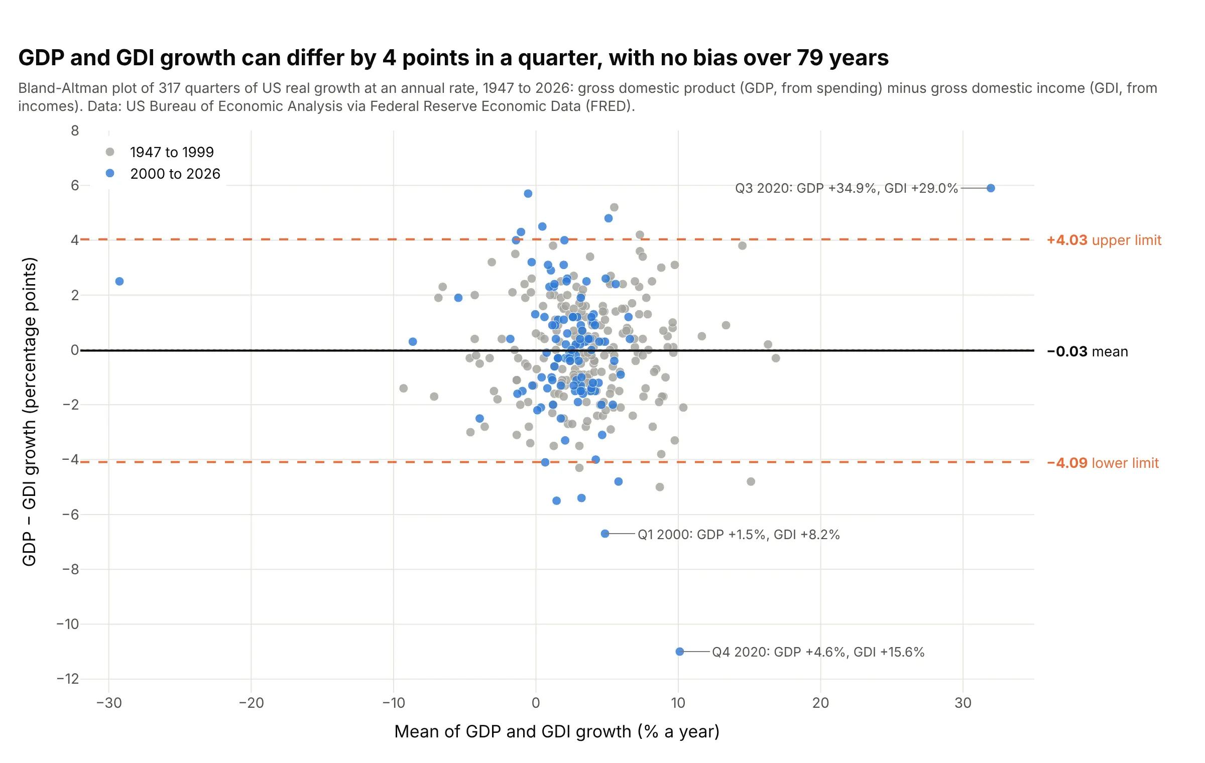
Bland-Altman plot of 317 quarters of US real growth, GDP minus GDI against their mean, 1947 to 2026: no bias (mean -0.03 points), limits of agreement at +4.03 and -4.09 points, and labels on Q4 2020 (GDP +4.6%, GDI +15.6%), Q1 2000 and Q3 2020

Gross domestic product (GDP) adds up spending and gross domestic income (GDI) adds up incomes, so in theory they measure the same thing. Over 317 quarters their growth rates show no bias at all, but 95% of quarters differ by up to about 4 percentage points, and in the fourth quarter of 2020 GDI grew 15.6% at an annual rate to GDP's 4.6%. Data: US Bureau of Economic Analysis (BEA) via Federal Reserve Economic Data (FRED).

Tip: color the points by era or label the extremes with their dates, so a time series in disguise still says when the disagreements happened.

Get the data from FRED series A191RL1Q225SBEA (real GDP, percent change at an annual rate) and
A261RL1Q225SBEA (real GDI, same units), quarterly (columns: quarter, gdp, gdi).

Build a plotly Bland-Altman plot of gdp - gdi against the mean, gray markers before 2000 and blue after,
the mean and limits labeled, and the three largest gaps annotated with the quarter and both growth rates.

6. NASA against the Met Office, two global temperature records

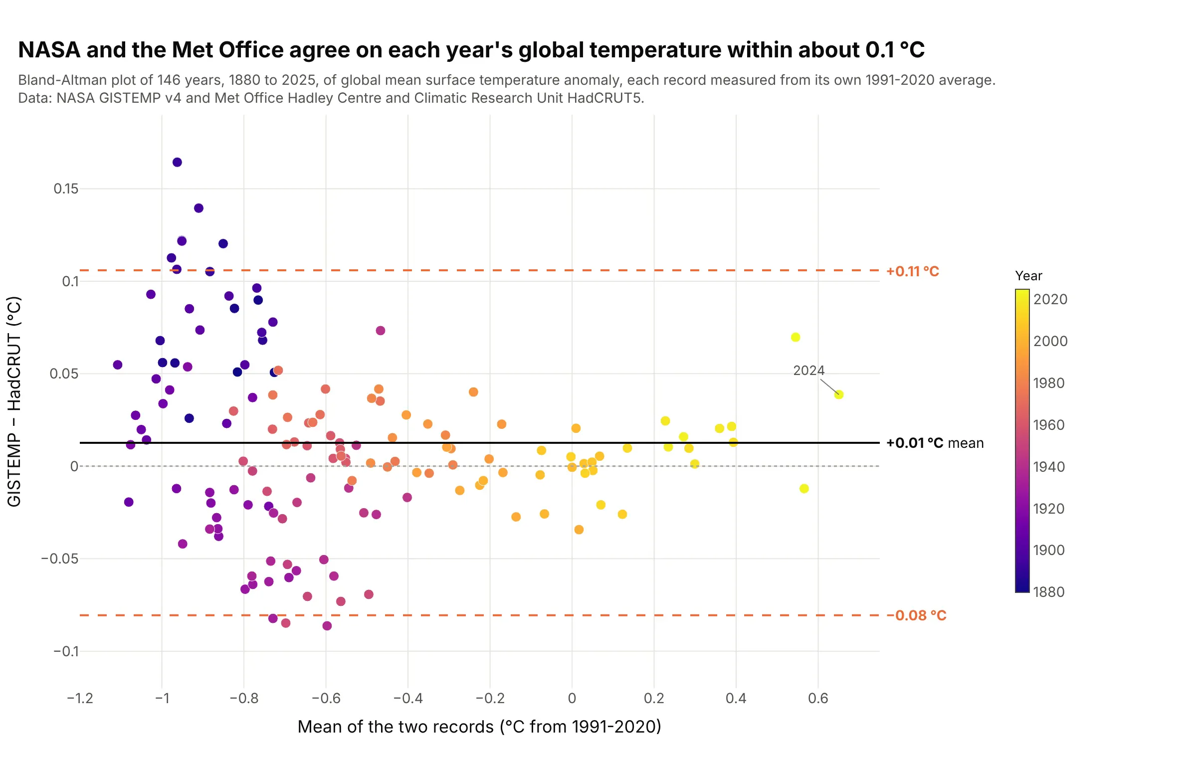
Bland-Altman plot of 146 years of global temperature anomaly, GISTEMP minus HadCRUT against their mean, colored by year: a mean difference of +0.01 degrees C and limits at +0.11 and -0.08, with the largest differences in purple points from before 1900 and recent years in yellow close to the mean line

NASA's Goddard Institute for Space Studies Surface Temperature Analysis (GISTEMP) and the Met Office and University of East Anglia's HadCRUT5 agree on each year's global temperature within -0.08 to +0.11 °C, once both are measured from their own 1991-2020 average. Coloring by year shows that 7 of the 10 years outside the limits are before 1900. Data: NASA GISTEMP v4 and Met Office Hadley Centre HadCRUT5.

Tip: put two records on a common baseline before you compare them, or the difference in baselines shows up as a bias.

Get the data from NASA GISTEMP v4 GLB.Ts+dSST.csv (annual J-D column) and the Met Office HadCRUT.5.1.0.0
analysis global annual summary series, 1880 to 2025, each re-expressed against its own 1991-2020 mean
(columns: year, gistemp, hadcrut).

Build a plotly Bland-Altman plot of gistemp - hadcrut against their mean, markers colored by year with
the Plasma colorscale and a colorbar, and the mean and limits labeled in °C.