Marginal Plots - A Complete Guide

TL;DR

• A marginal plot is a scatter plot (or a 2D histogram or density contour) with a small chart of each variable’s own distribution on its edges: a histogram, box plot, violin, or rug along the top for x and down the right side for y.
• Marginal plots are also known as joint plots (seaborn’s jointplot), marginal distribution plots, and scatter plots with marginal histograms, and are similar to scatter plots, 2D histogram contours, and scatter plot matrices.
• The edges count what the middle hides: when thousands of points land on top of each other, the scatter can’t show how many are there, and the histogram on the edge can.
• You can make one with Plotly in one line of code: px.scatter(df, x=..., y=..., marginal_x="histogram", marginal_y="histogram"), and every kind of seaborn’s jointplot (scatter, kernel density estimate (KDE), hist, hex, reg, and resid) has a Plotly equivalent.

What is a marginal plot?

Marginal plots look like this:

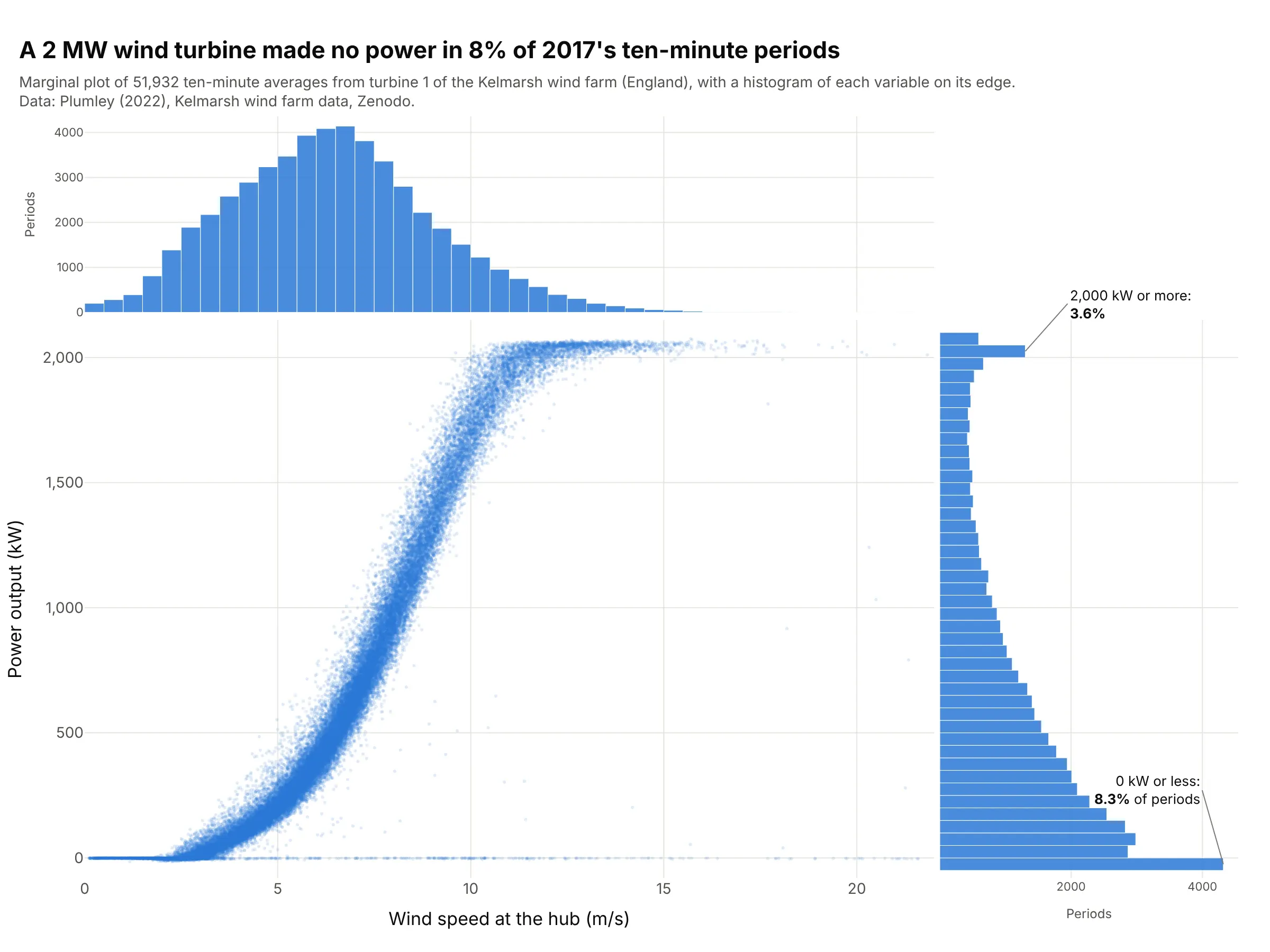
Data: Plumley (2022), Kelmarsh wind farm data, Zenodo, supervisory control and data acquisition (SCADA) data from turbine 1, a Senvion MM92 rated at 2,050 kW.

How do you read a marginal plot? In the example above, notice these things:

• The middle is an ordinary scatter plot: each of the 51,932 dots is one ten-minute period of 2017, placed by its wind speed and the power the turbine made. Together they trace the turbine’s power curve, which rises from about 3 m/s and flattens at full power above about 11 m/s.
• The histogram on top counts the periods at each wind speed, ignoring power. Most periods had light to moderate wind, with a median of 6.33 m/s, and very few had more than 15 m/s.
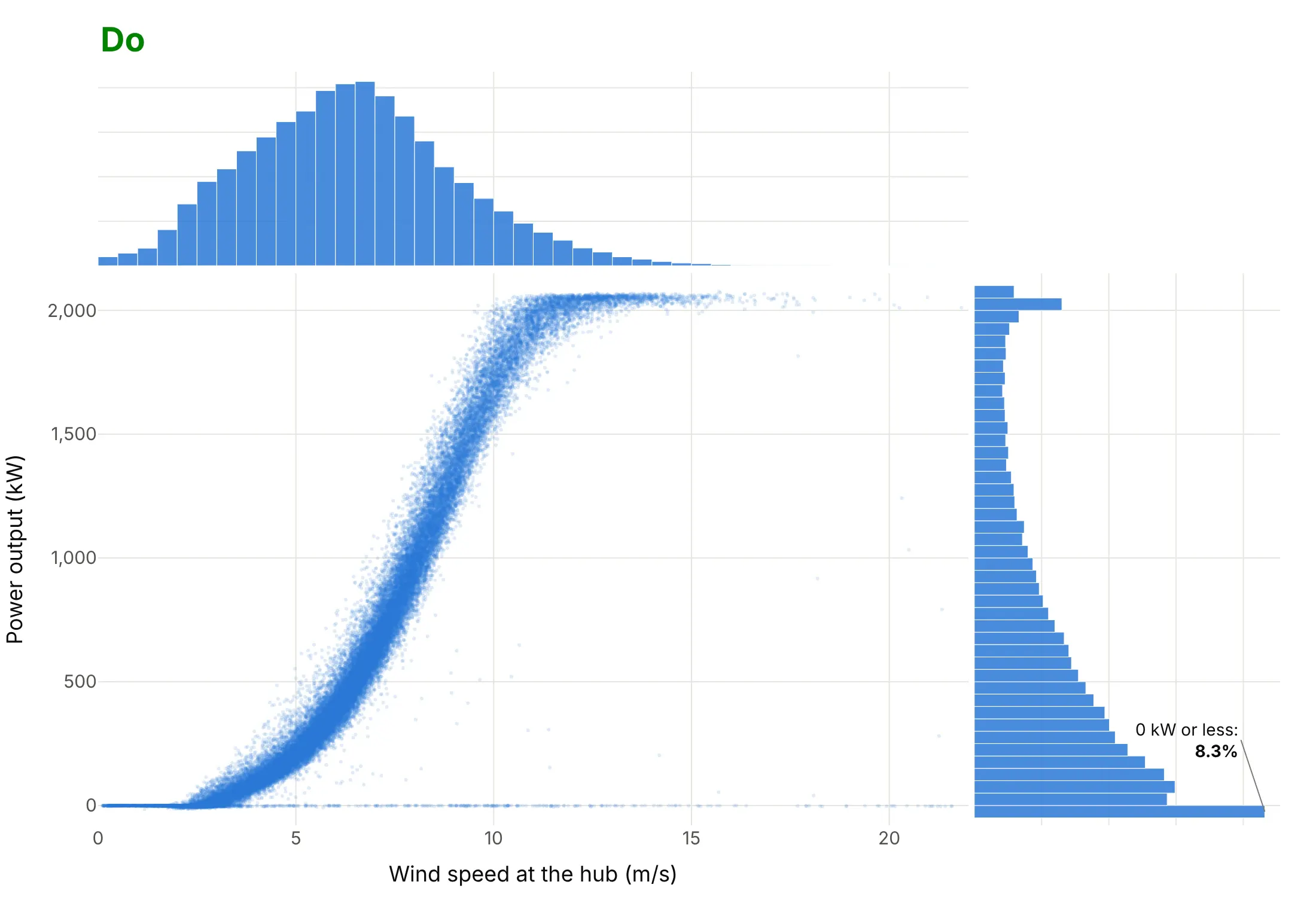
• The histogram on the right counts the periods at each power level, ignoring wind speed. Its tallest bar is at zero: in 4,333 periods (8.3%) the turbine made no power, mostly in winds under 3 m/s. In the scatter those periods are a thin line along the bottom, because they sit on top of each other.
• The second bump at the top of the right histogram is the 3.6% of periods at 2,000 kW or more, where the curve flattens and the dots pile up the same way.

It’s often used for charts like these:

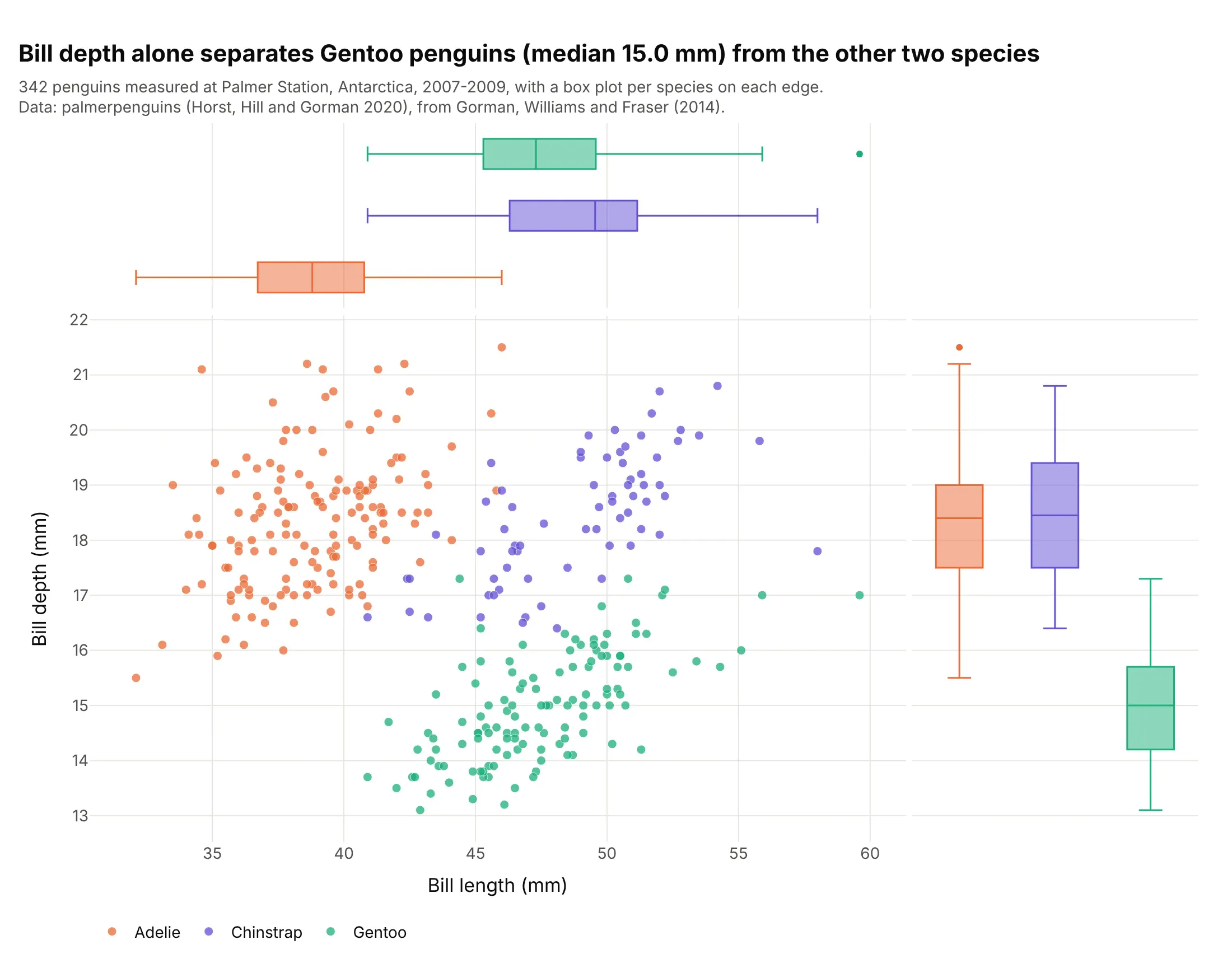
Groups. Colored by species, the edges get one box plot per species, and the right-hand boxes show that bill depth alone separates Gentoo penguins (median 15.0 mm) from the other two (18.4 mm). This is the dataset of seaborn’s jointplot documentation. Data: palmerpenguins (Horst, Hill, and Gorman 2020), from Gorman, Williams, and Fraser (2014).

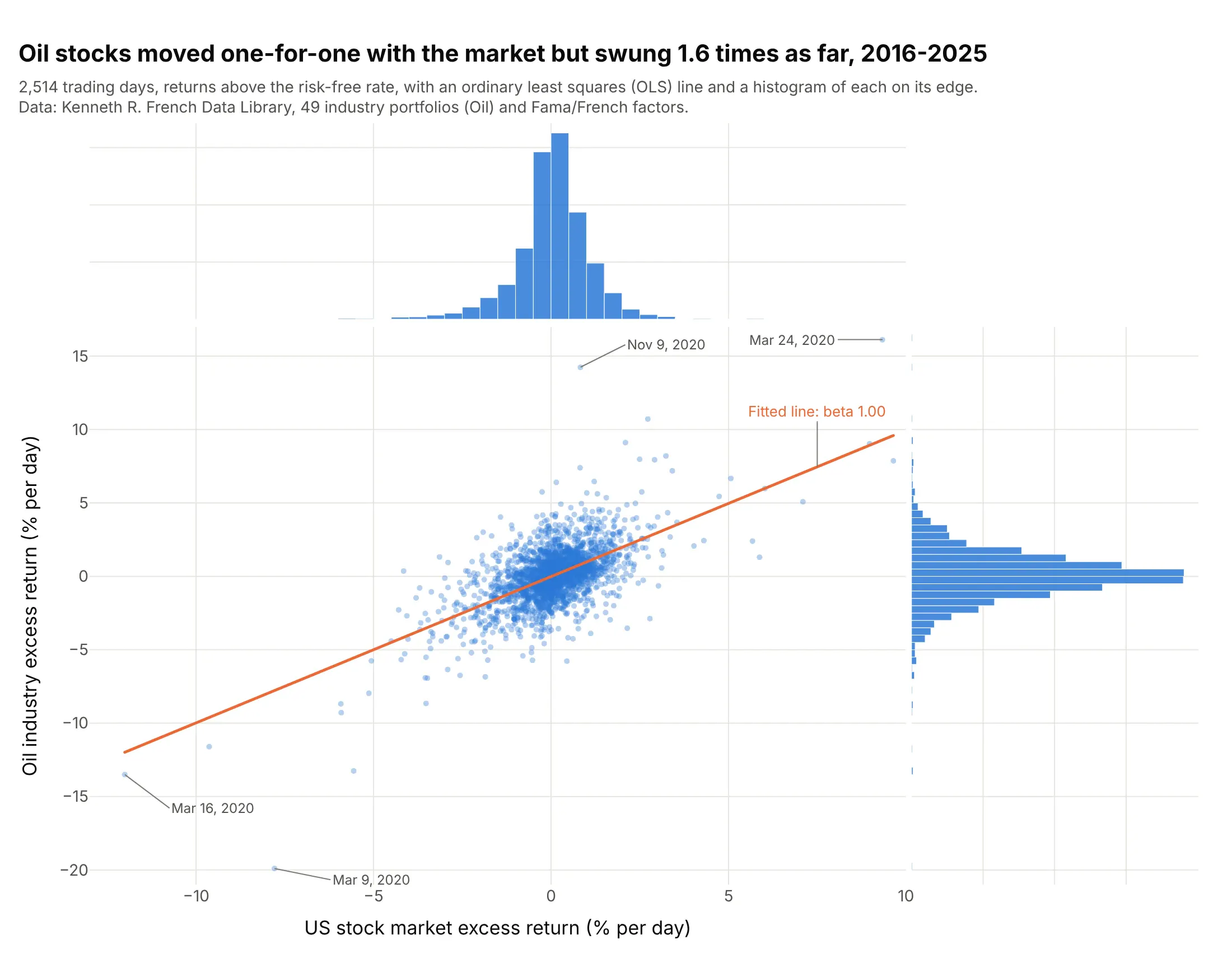
Regression and risk. The fitted line says oil stocks moved one-for-one with the market (beta 1.00), and the histograms on the edges show the other half of the story: oil’s daily returns spread 1.6 times as wide. Data: Kenneth R. French Data Library, 49 industry portfolios (Oil) and Fama/French factors, daily.

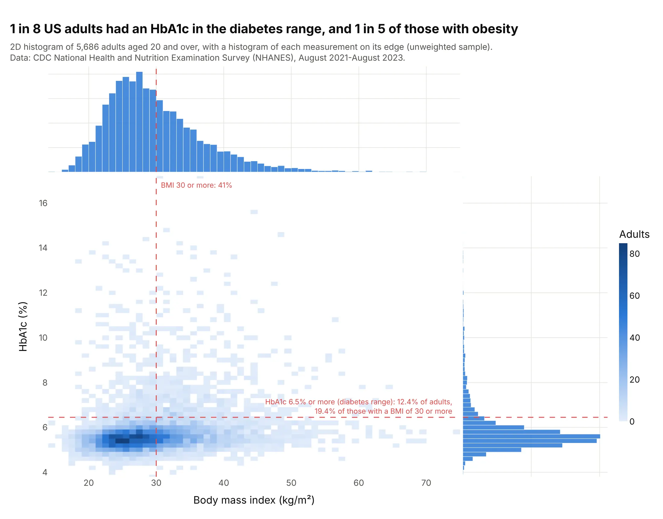
Clinical lab values. With 5,686 adults a scatter turns into a blob, so the middle is a 2D histogram, and the edges show each measurement against its clinical cut-off: 12.4% of adults had a glycated hemoglobin (HbA1c) in the diabetes range, and 19.4% of those with a body mass index (BMI) of 30 or more. Data: US Centers for Disease Control and Prevention (CDC), National Health and Nutrition Examination Survey (NHANES), August 2021 to August 2023.

What the edges add

A scatter plot shows how two variables move together, but it’s bad at showing how many points are in each place. Once points overlap, a spot with 10 points and a spot with 4,000 look the same. This is the turbine data from the top of the page without its edges:

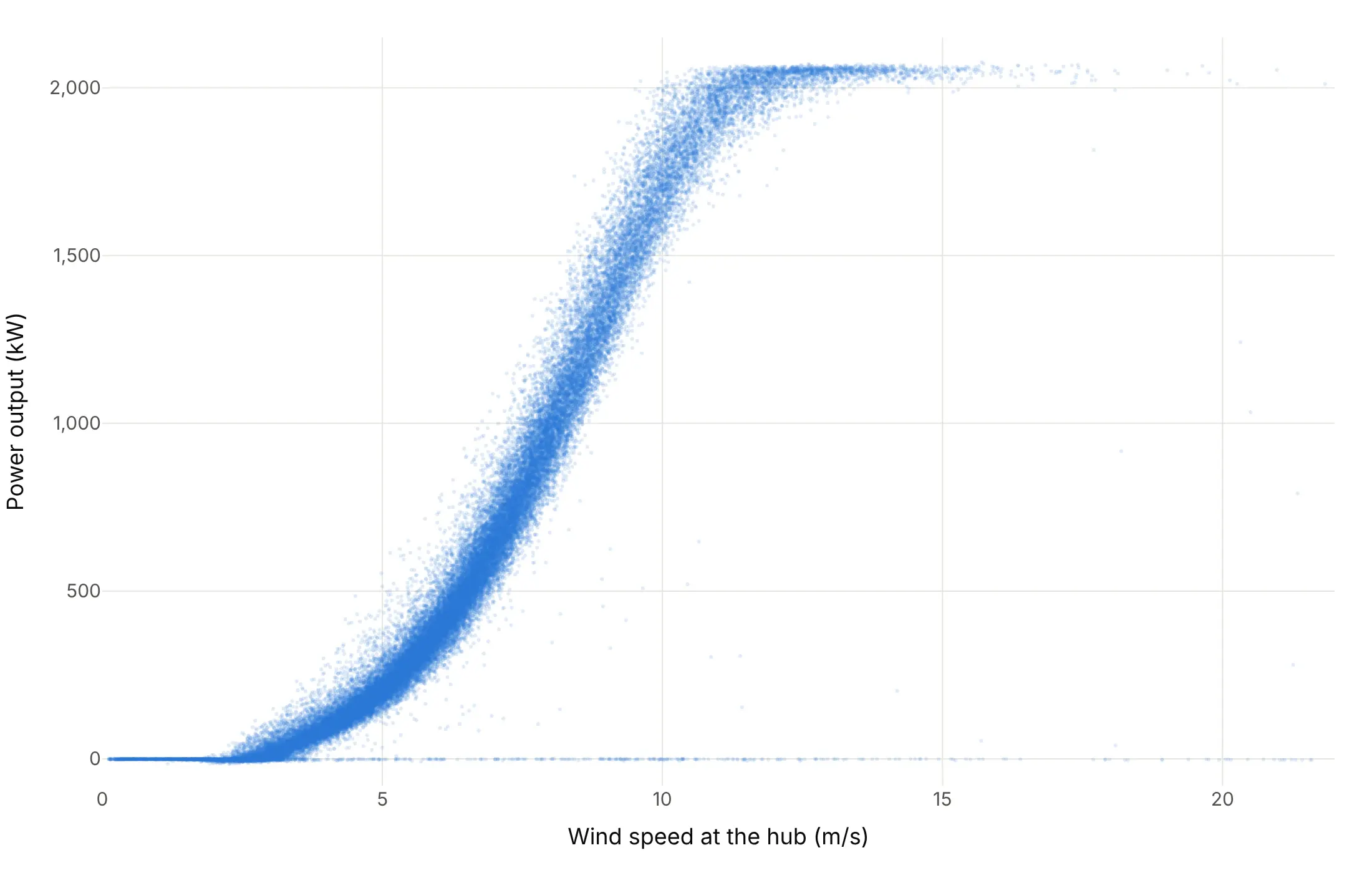
Nothing in it says that the thin line at 0 kW holds more periods than any other 50 kW band of the chart. The histogram on the right edge says so at once, because it counts.

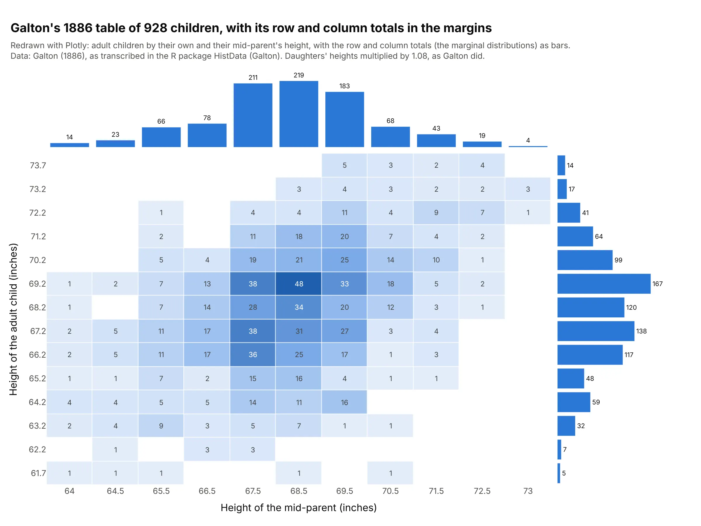
Statisticians call each variable’s own distribution its marginal distribution, and the name comes from tables: if you cross-tabulate two variables, the totals of each row and column are written in the margins of the table, and those totals are the distribution of one variable ignoring the other (Wikipedia). A marginal plot draws those totals as charts next to the scatter, so you see three things at once: the relationship in the middle and each variable alone on the edges. The edge charts share their axis with the middle, so a bar on the top histogram sits right above the points it counts, and zooming the middle zooms the edges with it.

seaborn’s jointplot in Plotly

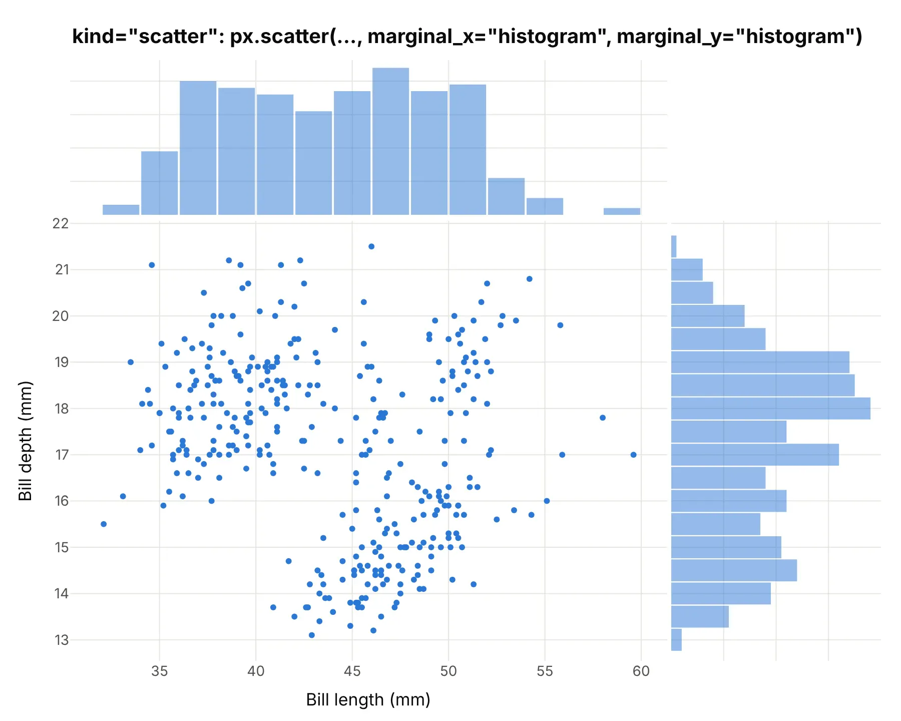
Many people first meet marginal plots as seaborn’s jointplot, which “draws a plot of two variables with bivariate and univariate graphs” and takes kind="scatter", "kde", "hist", "hex", "reg", or "resid". Each one has a Plotly equivalent. These are the same penguins seaborn’s documentation uses, drawn with Plotly Express.

kind="scatter" (the default) is px.scatter with marginal_x="histogram" and marginal_y="histogram":

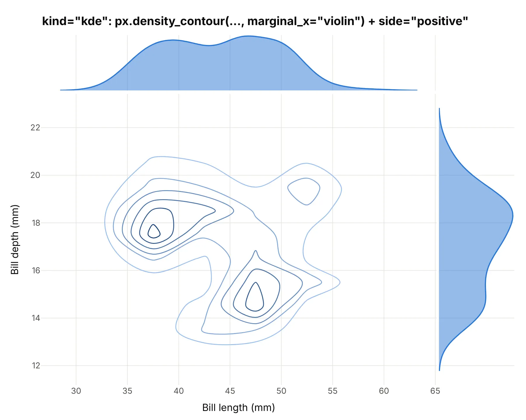
kind="kde" draws kernel density estimate (KDE) contours in the middle and a density curve on each edge. In Plotly, px.density_contour draws the contours from a 2D histogram, and marginal_x="violin" with side="positive" cuts each violin in half, which leaves a density curve:

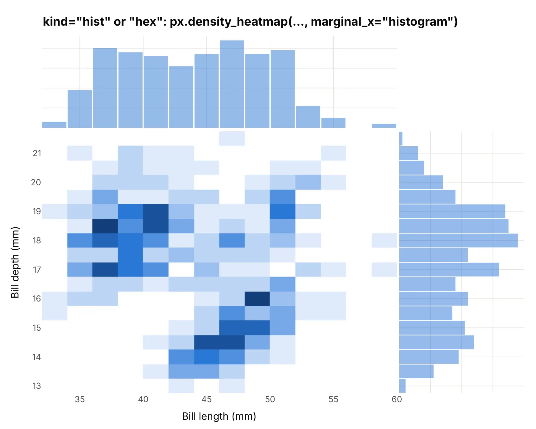
kind="hist" and kind="hex" count points in bins: squares for hist, hexagons for hex. px.density_heatmap with histogram marginals draws the square version; Plotly has no hexagon option in Plotly Express, and the hexbin plot guide shows how to draw hexagons:

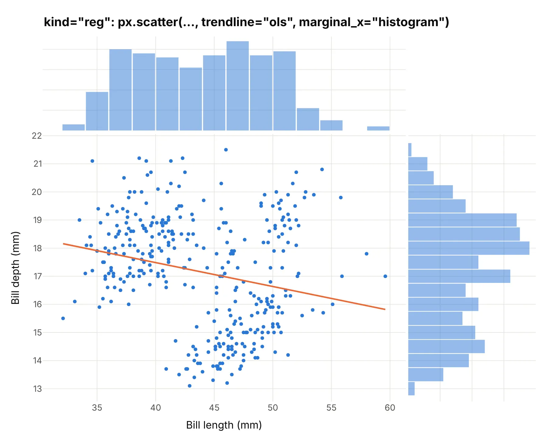
kind="reg" adds a regression line. Use trendline="ols" (ordinary least squares) with histogram marginals. seaborn also shades a confidence band around the line, which Plotly Express doesn’t draw:

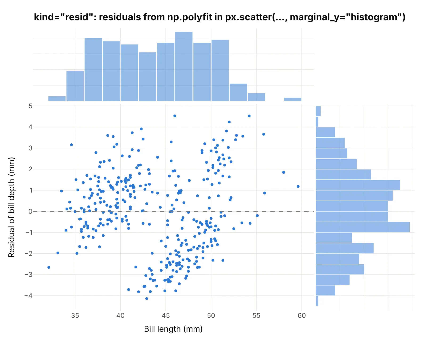
kind="resid" plots what’s left after the regression line: compute the residuals (for example with np.polyfit) and pass them as y. Here they show that one straight line through all three species leaves two separate clouds, so species belongs in the model:

seaborn’s hue= is Plotly’s color=, which splits every edge chart by group as in the penguin example above. Plotly also adds edge types seaborn’s jointplot doesn’t have: "box", "violin", and "rug" (one tick per point) on px.scatter, and "heatmap" on px.density_heatmap since Plotly 7.1.

A short history

The word comes from tables. Francis Galton’s 1886 study of heredity cross-tabulated 928 adult children by their own height and their parents’ average height, and the totals of a table like that, by row and by column, are its marginal distributions. Here is Galton’s table redrawn with Plotly from the transcription in the R package HistData, with the totals drawn as bars in the margins:

Drawing the margins next to a scatter plot became a standard command in statistics software: MATLAB’s scatterhist (“scatter plot with marginal histograms”), R’s ggExtra package with ggMarginal, seaborn’s jointplot, and Plotly Express’s marginal_x and marginal_y.

Alternatives to a marginal plot

Here’s the same year of turbine periods drawn six other ways. Some are better for the question, some worse, some just different:

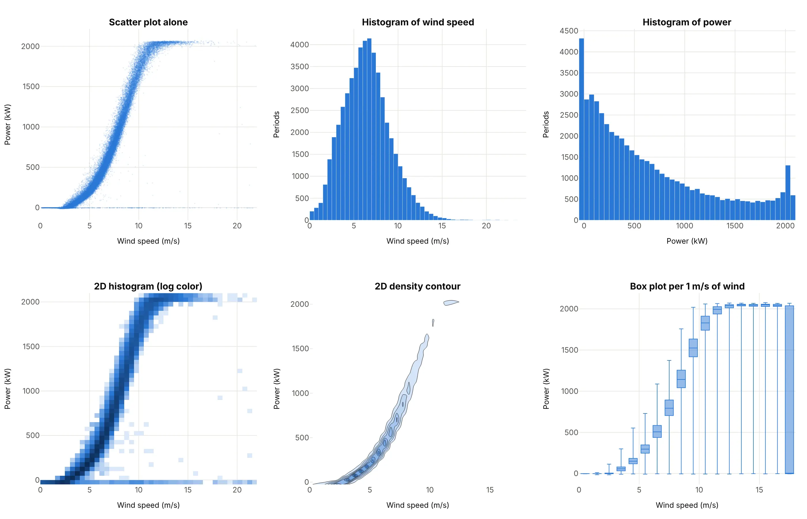
• Scatter plot alone (worse for counts). It shows the relationship as well as the marginal plot does, but not how many points are on the 0 kW line or at full power. It’s the better choice for a few hundred points that don’t overlap.
• Two separate histograms (worse). They show each distribution, but you can’t tell which wind speeds produced the periods at 0 kW. The marginal plot keeps both.
• 2D histogram (works too, often better for big data). Counting points in bins solves the overlap in the middle as well, and with a log color scale the 0 kW line shows up. It’s what the NHANES example above uses, with histograms on its edges.
• 2D density contour (different). It draws the smooth shape of the dense middle and drops the sparse points, which here hides both the 0 kW line and the periods at full power. Good for smooth, unimodal clouds.
• Box plots per bin of x (better for the power curve). One box for each 1 m/s of wind gives a cleaner power curve with its spread at each speed. It loses the individual points and the distribution of wind speed itself.

When you have more than two variables, a scatter plot matrix draws every pair with each variable’s histogram on the diagonal, which is the marginal plot idea for several variables at once.

How to make a marginal plot

With AI

ChatGPT, Claude Code, GitHub Copilot, Cursor, and other AI tools are excellent at writing Plotly code. Name Plotly in the prompt, and say which chart goes in the middle and which goes on each edge:

With Plotly Studio

Plotly Studio is a desktop app where you point an AI at a dataset and it builds charts and a Dash app around your questions. Ask for a marginal plot the same way:

Show a marginal plot of hourly demand against solar generation, with histograms on both edges, a log count axis on the solar histogram, and a dropdown to switch the edges between histograms, box plots, and violins.

Make a marginal plot in Python or JavaScript

This is the code AI tools write under the hood. In Python, Plotly Express adds the edge charts with two arguments:

The same two arguments work on px.density_heatmap and px.density_contour, which put a 2D histogram or contours in the middle for large data, and px.histogram takes one marginal= argument to put a box, violin, or rug above a histogram. trendline="ols" adds a regression line (it needs the statsmodels package).

In JavaScript, plotly.js draws a marginal plot from a scatter trace and two histogram traces on axes that share their ranges with the scatter’s:

matches keeps each edge chart’s axis locked to the middle one, so zooming the scatter zooms its edges too.

Share it

Every Plotly chart has a Share chart button (the cloud icon in its toolbar) that uploads it to Plotly Cloud and gives you a link. Only you can see it until you change its visibility.

For a live app, put the chart in a Dash app and publish it with the Plotly Cloud command-line interface (CLI). Coding agents can run these commands for you:

If your data has to stay in your own cloud or data center, publish to Dash Enterprise instead.

Dos and don’ts

A marginal plot only helps if the middle shows the relationship and the edges count, so most of the work is the markers and the choice of edge chart. Here is the turbine year both ways, in the same color.

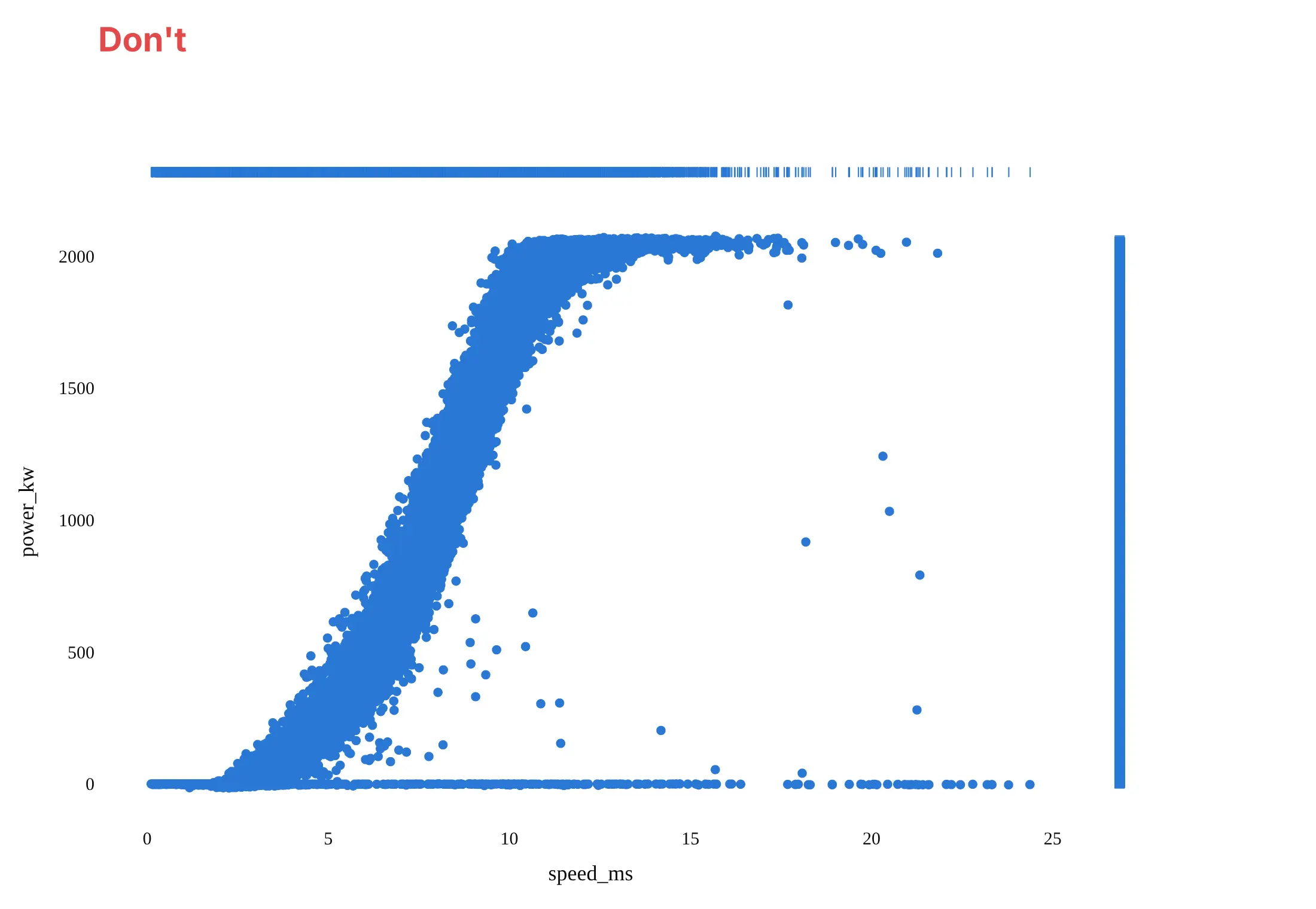
Don’t draw 52,000 points with big opaque markers, which merge into a solid band, put rug plots on the edges of that many points, which turn into solid bars that count nothing, leave the raw column names speed_ms and power_kw as axis titles, or use a default serif font:

Do use small, partly transparent WebGL markers so dense areas look darker, put histograms with fixed bin widths on the edges, write axis titles in words with units, and label the pile-up the edges reveal:

Checklist

Do

• Match the edge chart to the number of points: rug for under a few hundred, histogram, box, or violin above that.
• Set the same bin width for both edges when the two variables share units, so their spreads compare directly, as in the oil and market example.
• Switch the middle to px.density_heatmap or px.density_contour once points overlap into a blob.
• Color by group and let the edges split by group, with one box or overlaid histogram per group.
• Use a log axis, or plot log10 values with readable tick labels, for data that spans several powers of ten.

Don’t

• Read the edge histograms as the relationship; they show each variable alone, and two very different scatters can have the same edges.
• Overlay the histograms of groups with very different sizes without checking that the small group is still visible.
• Add a marginal plot to a scatter of 30 points where every point can already be seen.

Options to customize

For reference, these are the options that matter most. The full lists are in Plotly’s marginal plots documentation and the px.scatter reference.

1. marginal_x, marginal_y: "histogram", "box", "violin", or "rug" on px.scatter, px.density_heatmap, and px.density_contour; "heatmap" too on px.density_heatmap.
2. marginal on px.histogram: one box, violin, or rug above a histogram.
3. color: splits the points and every edge chart by group.
4. trendline="ols" (or "lowess") with trendline_color_override: a regression line in the middle.
5. render_mode="webgl": WebGL markers for tens of thousands of points or more.
6. opacity and marker.size: small, transparent markers so overlap reads as density.
7. xbins, ybins via fig.update_traces(..., selector=dict(type="histogram")): fixed bin widths on the edges.
8. side="positive", points=False on the violin traces: half violins, which work as density curves.
9. boxpoints on the box traces: "outliers", False, or "all".
10. barmode="overlay" with trace opacity: overlaid rather than stacked group histograms.
11. log_x, log_y: log axes, which the box, violin, and rug edges follow.
12. fig.update_xaxes(..., selector=dict(anchor="y2")): style or relabel one edge’s count axis, for example a log count axis for a pile-up.

More marginal plot examples

Six more marginal plots built from real public data, each with its source, the technique that makes it work, and a prompt to rebuild it.

1. Old Faithful’s eruptions, with rug plots

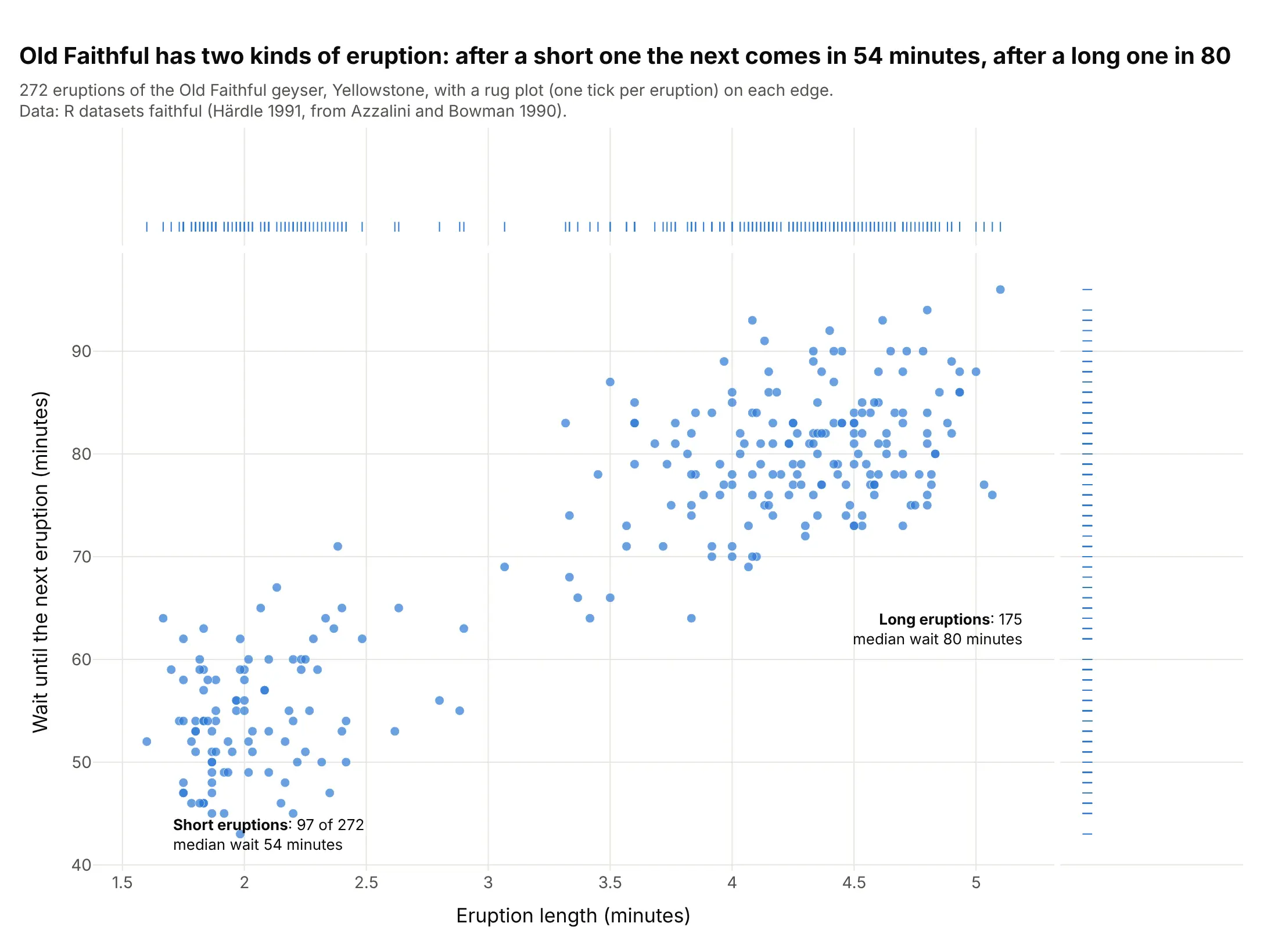
Old Faithful has two kinds of eruption, and the rugs on both edges show two groups of ticks with a gap between them. After the 97 short eruptions the next came in a median of 54 minutes, after the 175 long ones in 80. Data: R datasets::faithful (Härdle 1991, from Azzalini and Bowman 1990).

Tip: with a few hundred points, use marginal_x="rug", which shows every value as a tick instead of binning them.

2. Solar generation on the Texas grid, with a log count axis

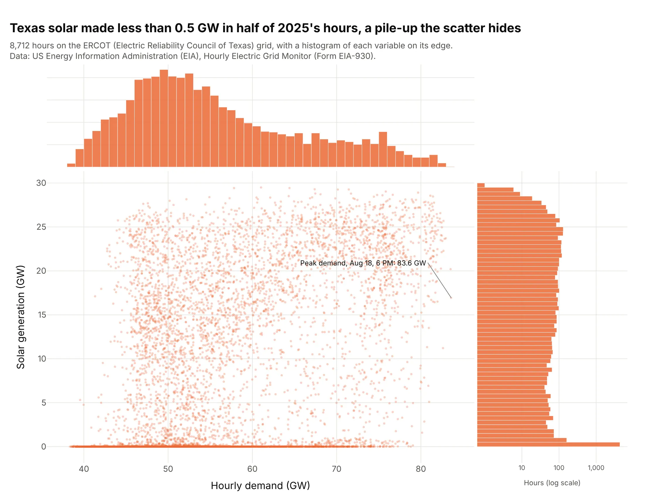
Solar on the Electric Reliability Council of Texas (ERCOT) grid made less than 0.5 GW in 50.1% of 2025’s hours, all of them between 6 PM and 8 AM, and in the scatter those hours are one line along the bottom. Demand peaked at 83.6 GW on August 18 at 6 PM, with 16.9 GW of solar. Data: US Energy Information Administration (EIA), Hourly Electric Grid Monitor (Form EIA-930).

Tip: give the edge with a pile-up a log count axis, so the other bars stay visible next to it.

3. Wind and waves at an offshore buoy, with violins

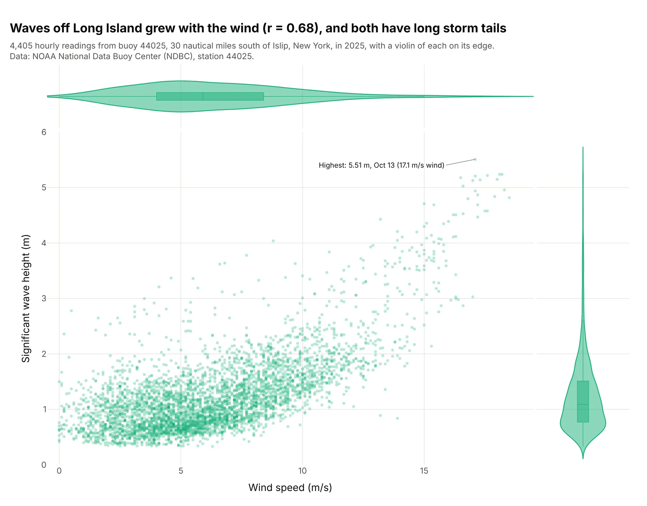
Waves 30 nautical miles south of Long Island grew with the wind (correlation r = 0.68), and both violins have long tails from a few storm hours. The highest significant wave height of 2025, 5.51 m, came on October 13 in a 17.1 m/s wind. Data: National Oceanic and Atmospheric Administration (NOAA), National Data Buoy Center, station 44025.

Tip: set box_visible=True on the violin edges, so the median and quartiles are marked inside each shape.

4. Exoplanets by discovery method, on log scales

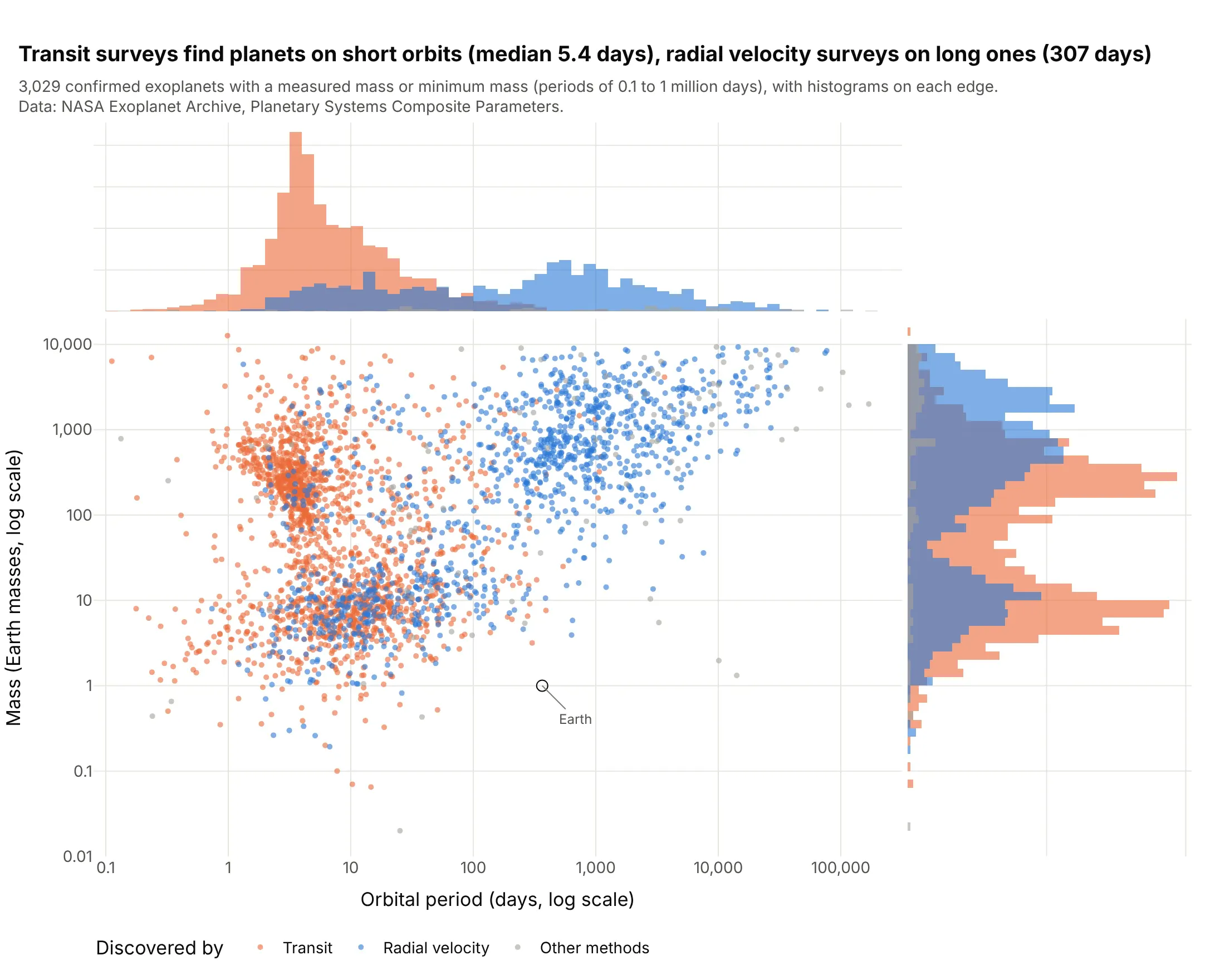
Transit surveys find planets on short orbits (median 5.4 days) and radial velocity surveys planets on long ones (307 days), and the colored period histograms on top barely overlap. Of the transit planets, 66.8% orbit in under 10 days. Data: NASA Exoplanet Archive, Planetary Systems Composite Parameters, planets with a measured mass or minimum mass.

Tip: for data spanning many powers of ten, plot log10 values so the histogram bins are even, and write the tick labels back in the original units.

5. Clinical trial size and duration by phase, with box plots

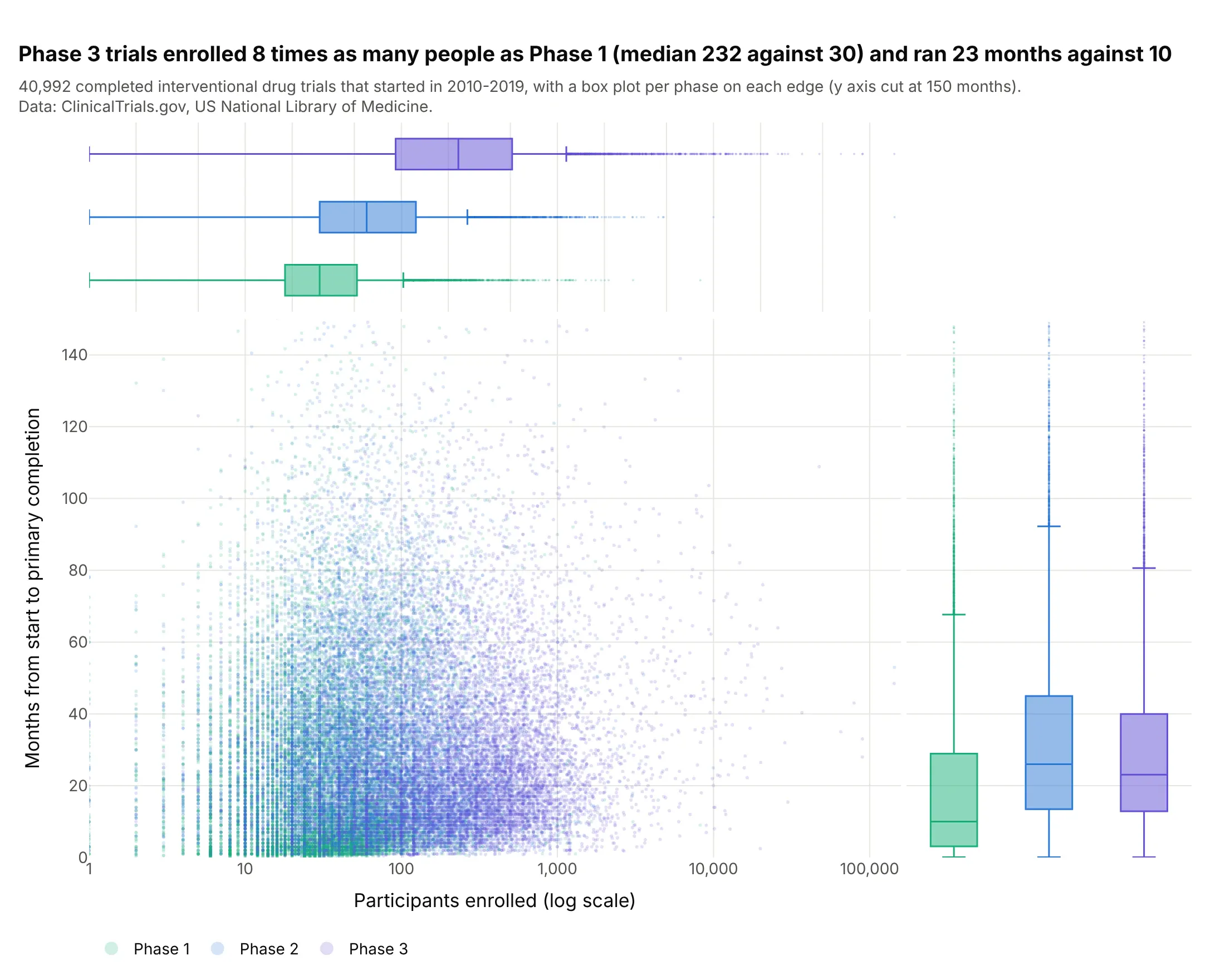
Phase 3 drug trials enrolled eight times as many people as Phase 1 (median 232 against 30) and took 23 months to their primary completion against 10, while Phase 2 took the longest, 26 months. In the middle, 41,000 trials overlap into one cloud; the boxes on the edges separate the phases. Data: US National Library of Medicine, ClinicalTrials.gov API, completed interventional trials.

Tip: with color= and marginal_x="box", each group gets its own box on each edge, which compares groups better than the overlapping points do.

6. The S&P 500 and the VIX, on a density contour

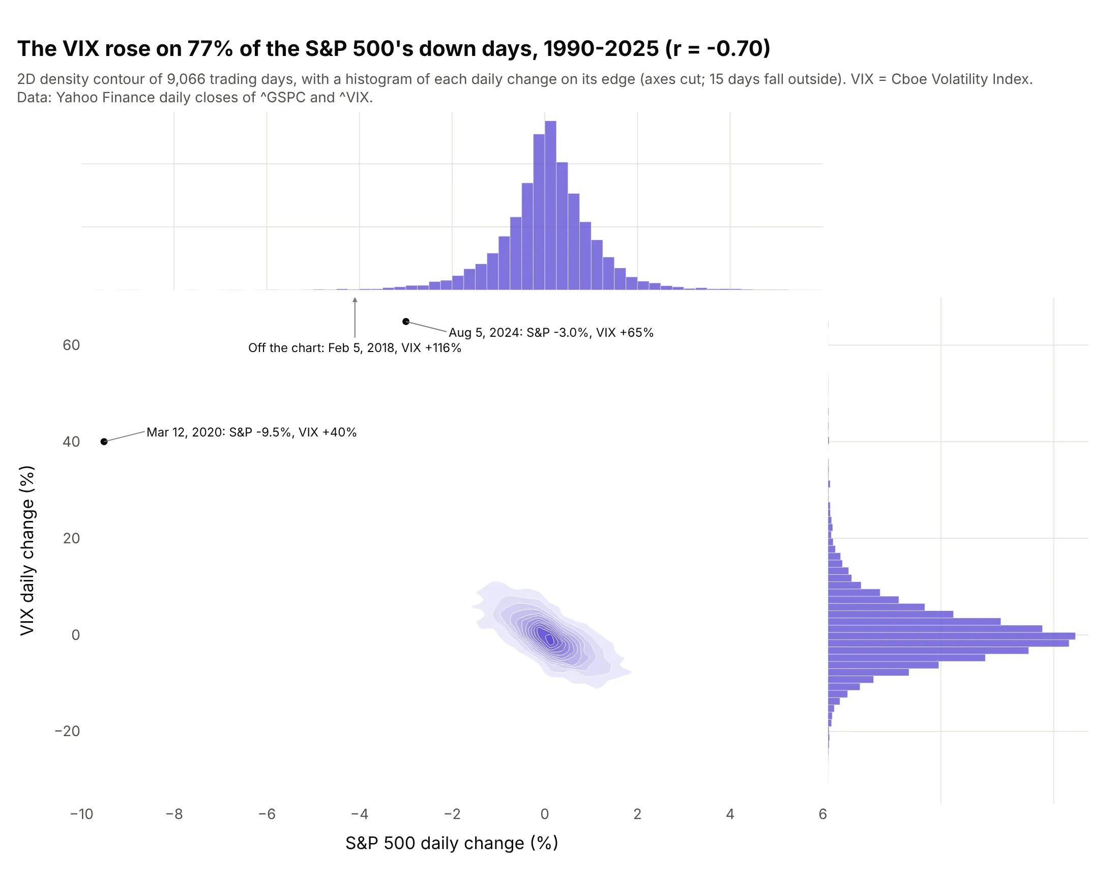
The Cboe Volatility Index (VIX), the market’s expected volatility from option prices, rose on 77% of the S&P 500’s down days from 1990 to 2025 (r = -0.70). The edges show its daily changes are 6.3 times as wide as the S&P’s and skewed up, with the largest rise in the data, +116%, on February 5, 2018. Data: Yahoo Finance daily closes of ^GSPC and ^VIX (VIX methodology).

Tip: in px.density_contour, set contours_coloring="fill" and label the extreme days as points on top, because the contours drop them.