Chris Parmer

November 4, 2026

Q-Q Plots - A Complete Guide

TL;DR

A Q-Q plot (quantile-quantile plot) sorts your data and draws each value against the value a reference distribution would put in the same position, so if the data follow that distribution, the points fall on a straight line.
Q-Q plots are also known as quantile-quantile plots and probability plots, and against a normal distribution as normal probability plots or normal plots. They are similar to probability-probability (P-P) plots, empirical cumulative distribution function (ECDF) plots, histograms and density plots.
Read the ends first: an S shape means heavy tails (stock and oil returns), a curve bending up at the right means right skew, a few points far off the line are outliers, and two straight runs with a jump mean two groups.
They are the standard check of regression residuals, the way genetic association studies show whether their p-values are inflated, and a quick way to compare two samples of any size.
You can make a Q-Q plot with Plotly in Python from scipy.stats.probplot or statsmodels' ProbPlot, which compute the points, and a go.Scatter trace with a reference line.

What is a Q-Q plot?

Q-Q plots look like this:

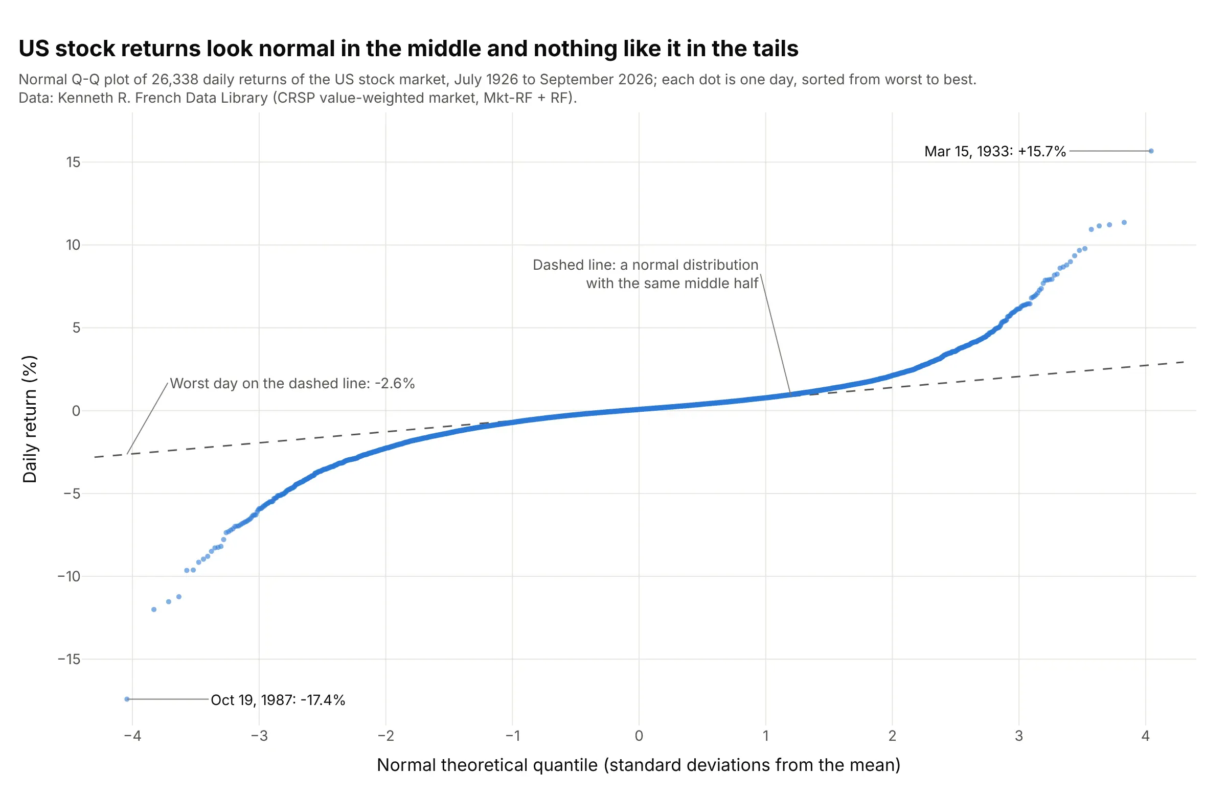
Normal Q-Q plot of 26,338 daily returns of the US stock market from July 1926 to September 2026: the points follow a dashed normal line in the middle and bend away from it at both ends in an S shape, with October 19, 1987 at -17.4% where the line expects -2.6%, and March 15, 1933 at +15.7%

Data: Kenneth R. French Data Library, daily return of the Center for Research in Security Prices (CRSP) value-weighted US stock market (the market's excess return plus the risk-free rate).

How do you read a Q-Q plot? In the example above, notice these things:

Each dot is one of 26,338 trading days, sorted from the worst to the best. Its height is the day's return, and its x position is where a day of that rank would fall in a normal distribution, in standard deviations.
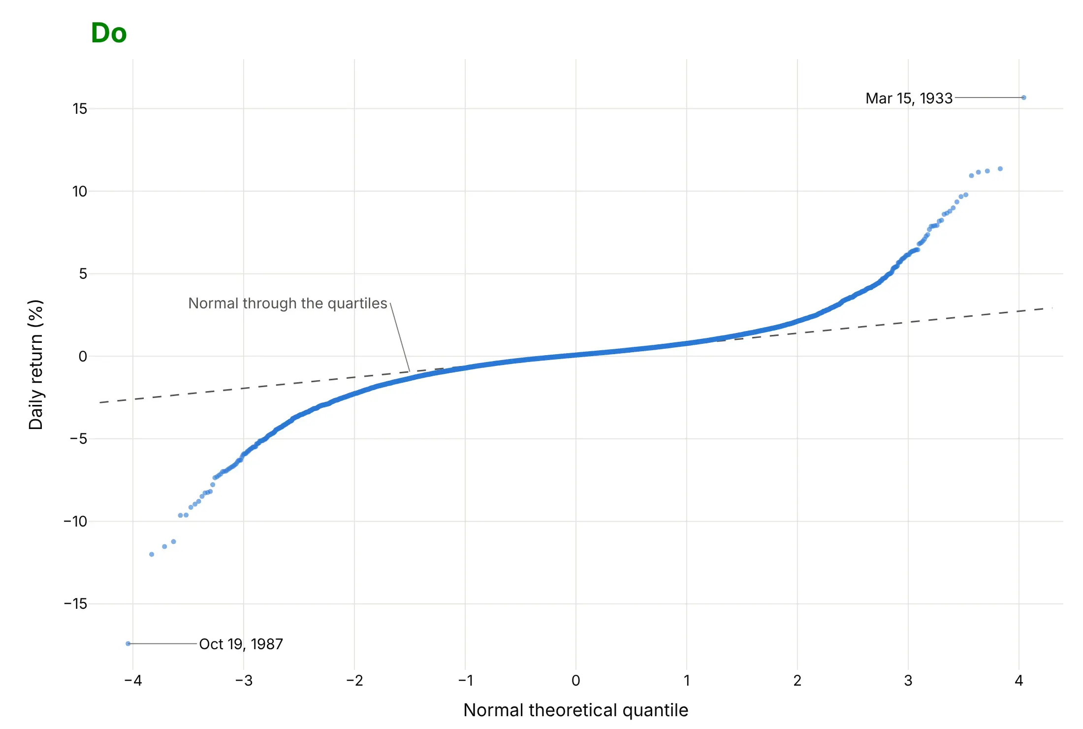
The dashed line is a normal distribution drawn through the data's quartiles, so it describes the middle half of the days. Between about -1.5 and +1.5 on the x axis, the dots sit on it, which means ordinary days look normal.
Both ends bend away from the line, the left end down and the right end up. That S shape is what heavy (or fat) tails look like: at -3 on the x axis the data are at -5.9% where the line gives -1.9%.
The extreme points are single days. October 19, 1987 fell 17.4%, where the line puts the worst of 26,338 normal days at 2.6%. 51 days fell 5 standard deviations or more, where a normal distribution expects 0.008.

It's often used for charts like these:

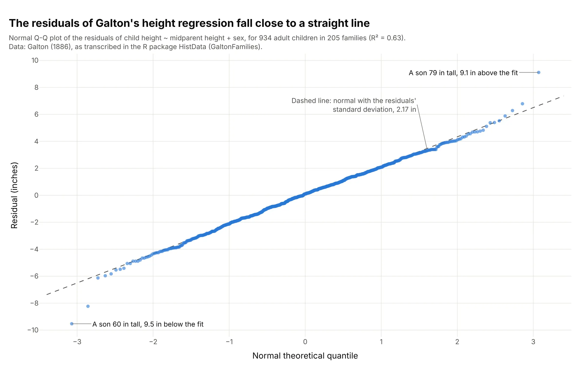
Normal Q-Q plot of the residuals of a regression of 934 children's heights on their parents' heights and sex, from Galton's 1886 data: the points lie along a straight dashed line from about -6 to +6 inches, with one son 9.5 inches below the fit and one 9.1 inches above it

Regression residuals. The residuals of Galton's height regression (R² = 0.63) follow the line closely, so a normal model fits, with two sons 9.5 and 9.1 inches from their predicted height at the ends. Data: Galton (1886), as transcribed in the R package HistData (GaltonFamilies).

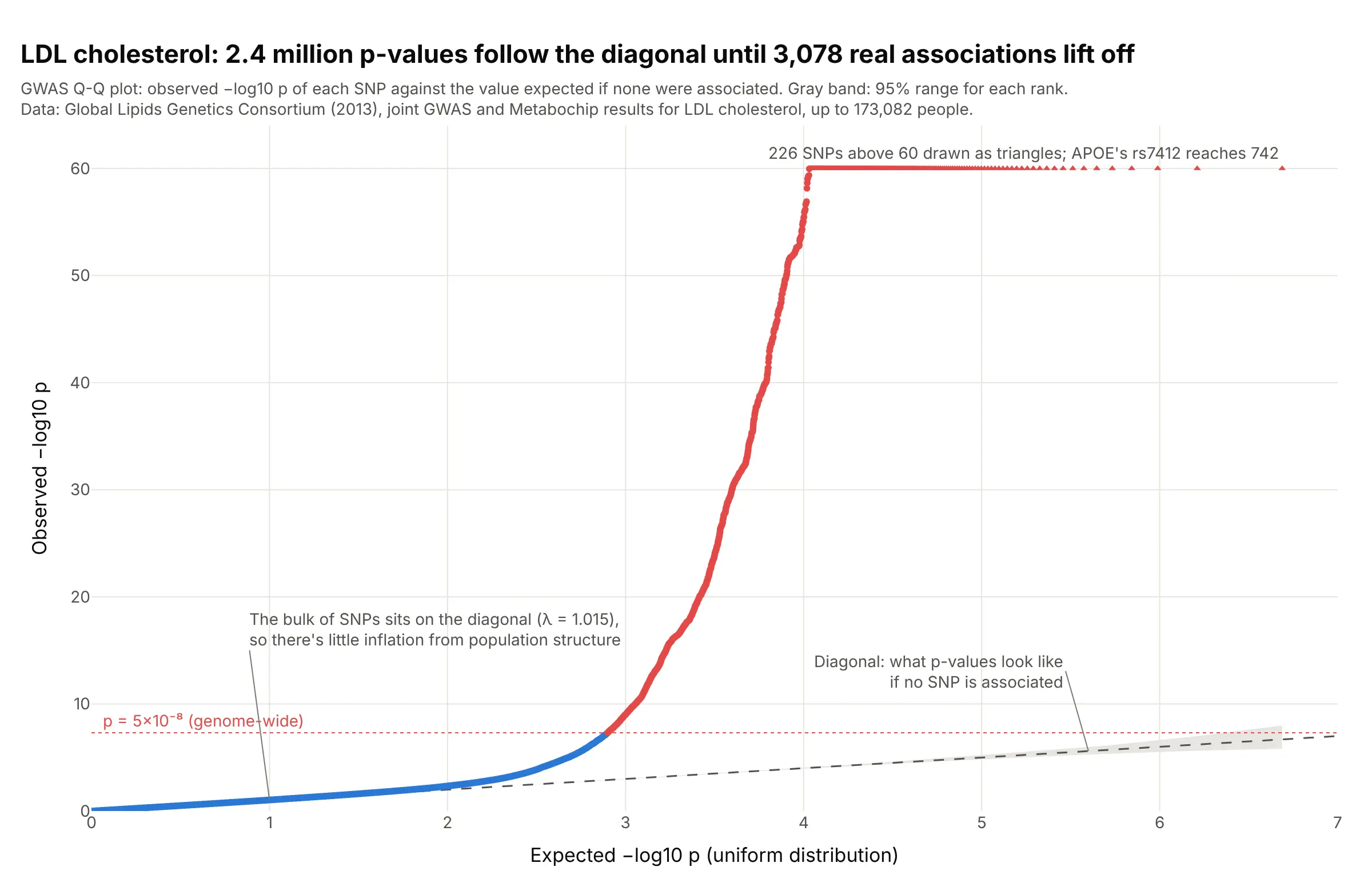
Genome-wide association study (GWAS) Q-Q plot of 2.4 million single-nucleotide polymorphisms (SNPs) tested for low-density lipoprotein (LDL) cholesterol: observed against expected -log10 p, with points close to the dashed diagonal at first, then lifting off in red above the genome-wide line, and 226 SNPs capped as triangles at 60 because APOE's rs7412 reaches 742

Genome-wide association studies (GWAS). The bulk of 2.4 million low-density lipoprotein (LDL) cholesterol p-values, one per single-nucleotide polymorphism (SNP), sits on the diagonal (genomic control λ = 1.015), so there's little inflation, and 3,078 SNPs past p = 5×10⁻⁸ lift off at the top. Data: Global Lipids Genetics Consortium (2013), joint GWAS and Metabochip results for LDL cholesterol.

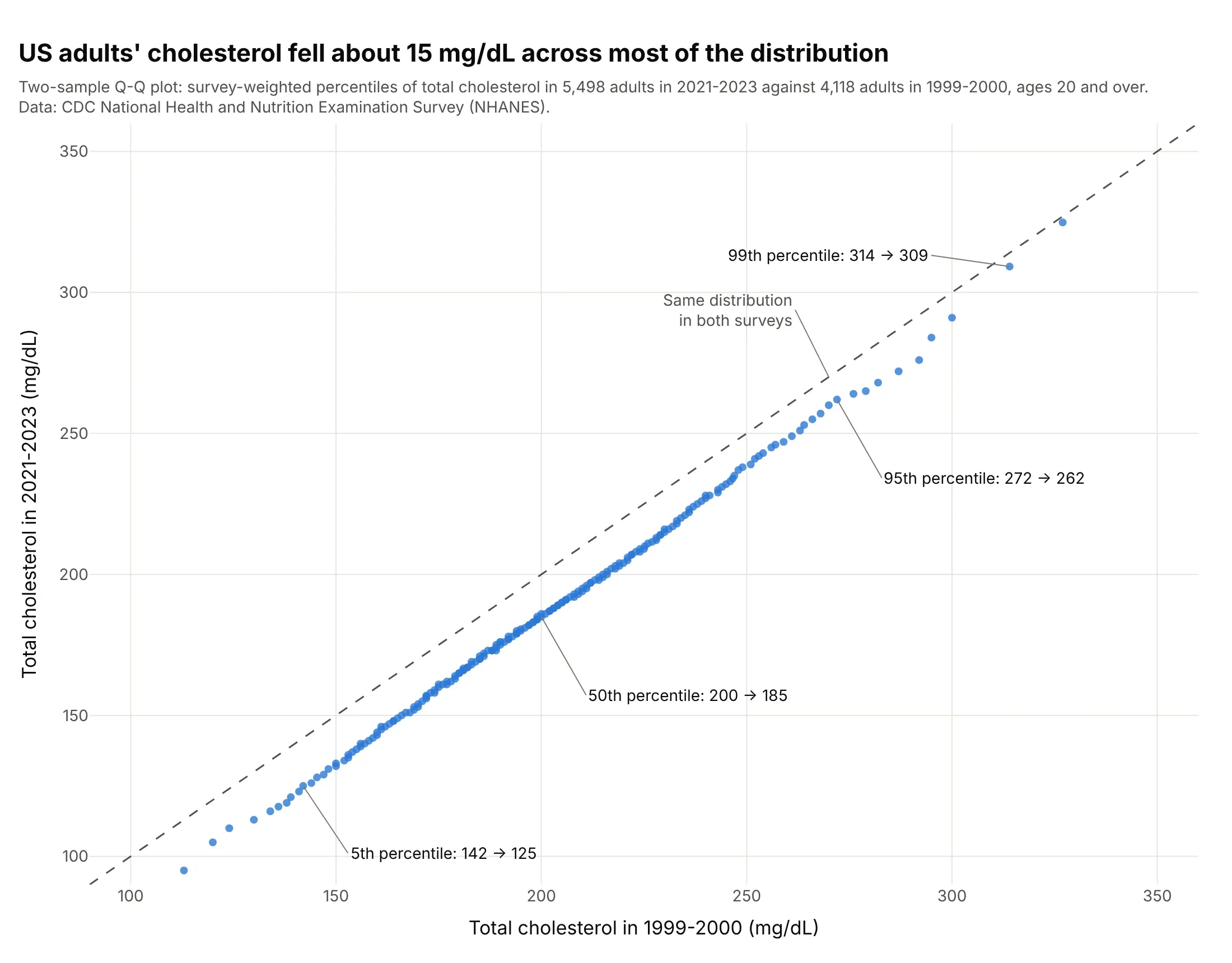
Two-sample Q-Q plot of survey-weighted percentiles of total cholesterol for US adults in 2021-2023 against 1999-2000: the points run parallel to and below the diagonal, with the median falling from 200 to 185 mg/dL and the 99th percentile from 314 to 309

Comparing two samples. Each percentile of US adults' cholesterol in 2021-2023 sits about 15 mg/dL below the same percentile in 1999-2000 (median 200 to 185), with a smaller drop at the top. Data: US Centers for Disease Control and Prevention (CDC), National Health and Nutrition Examination Survey (NHANES).

What Q-Q plots look like for different distributions

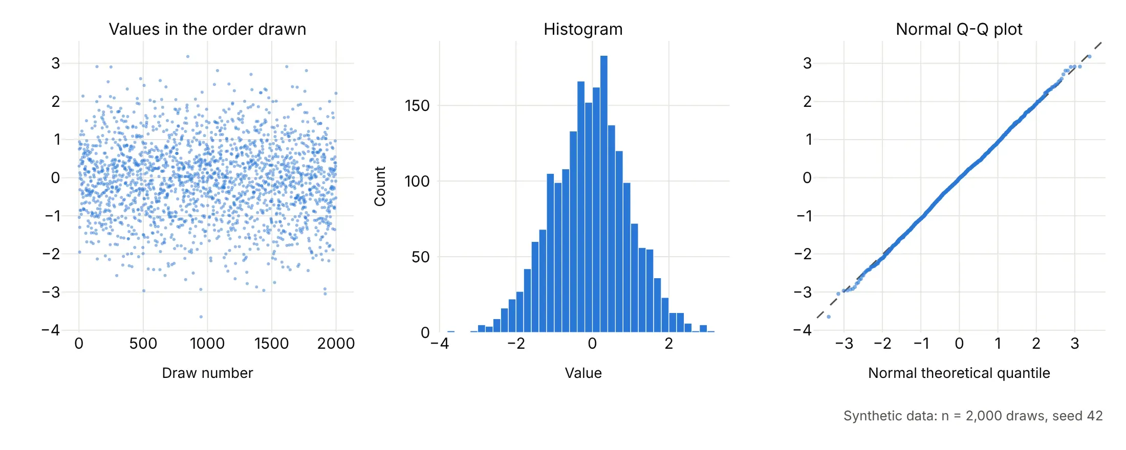
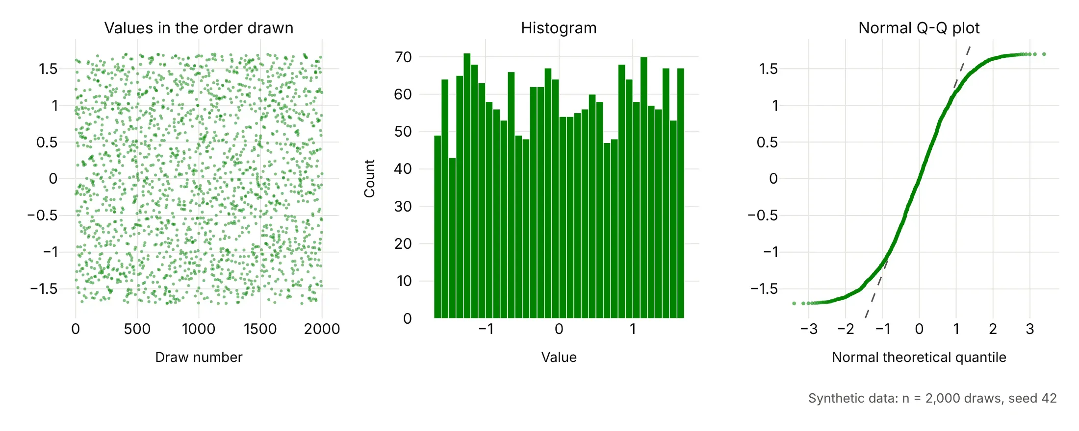
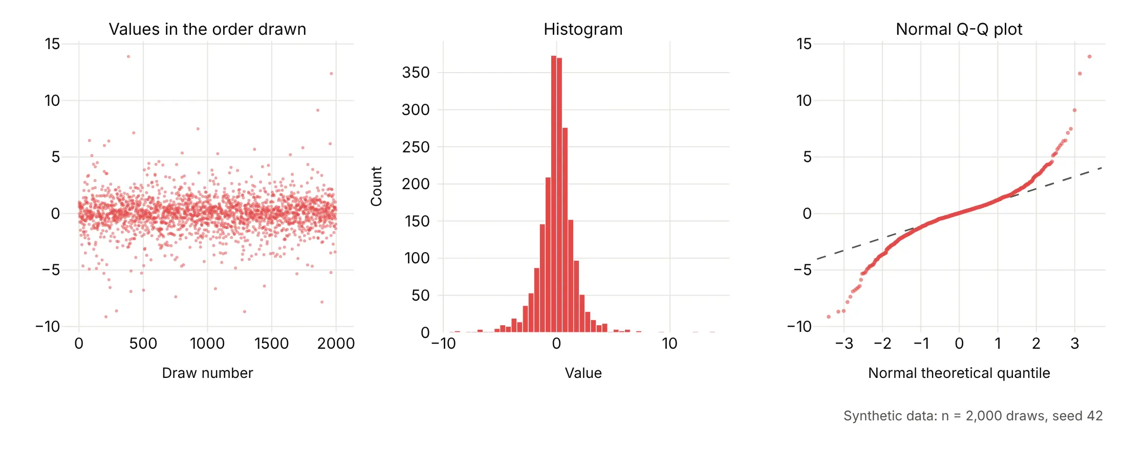
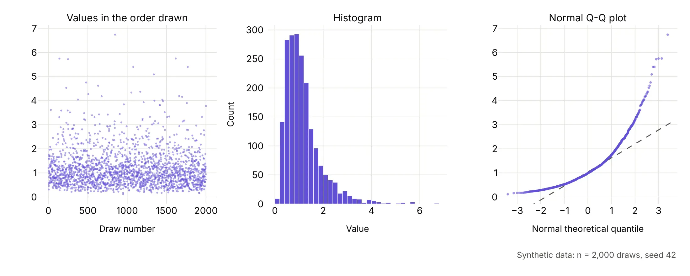
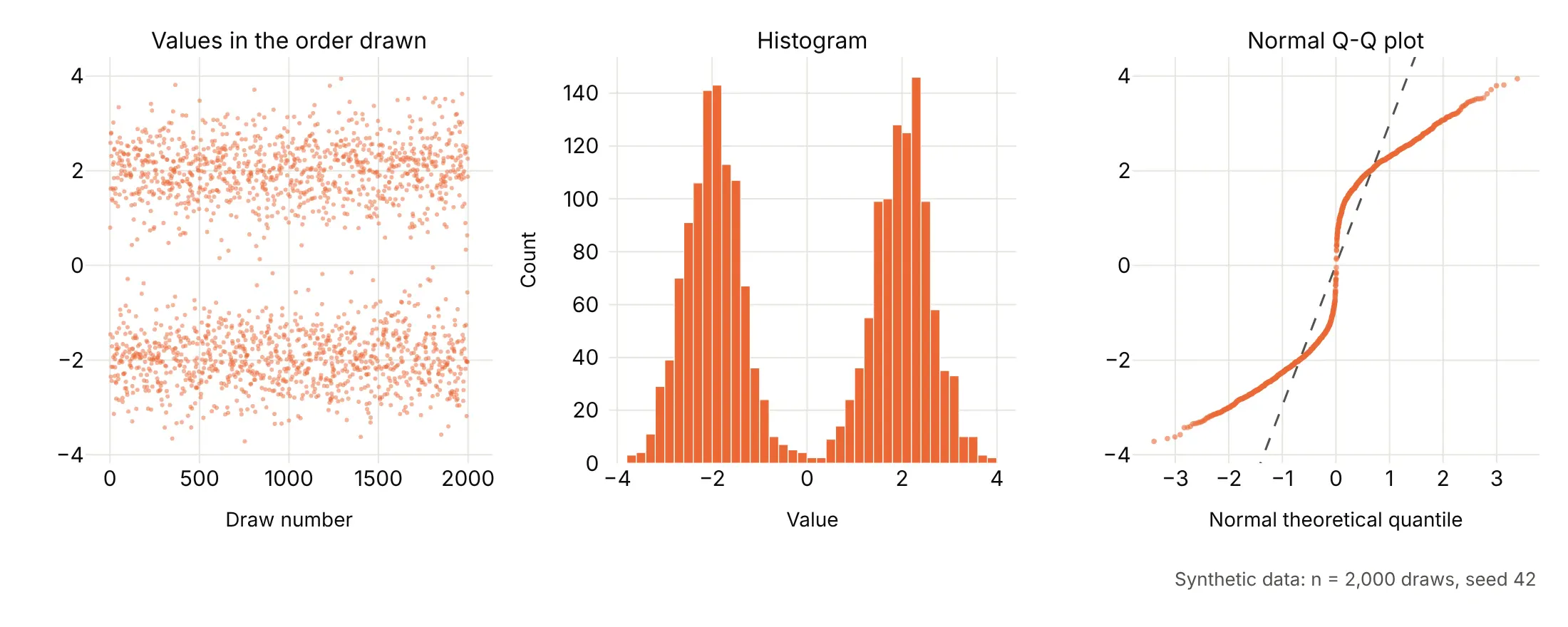
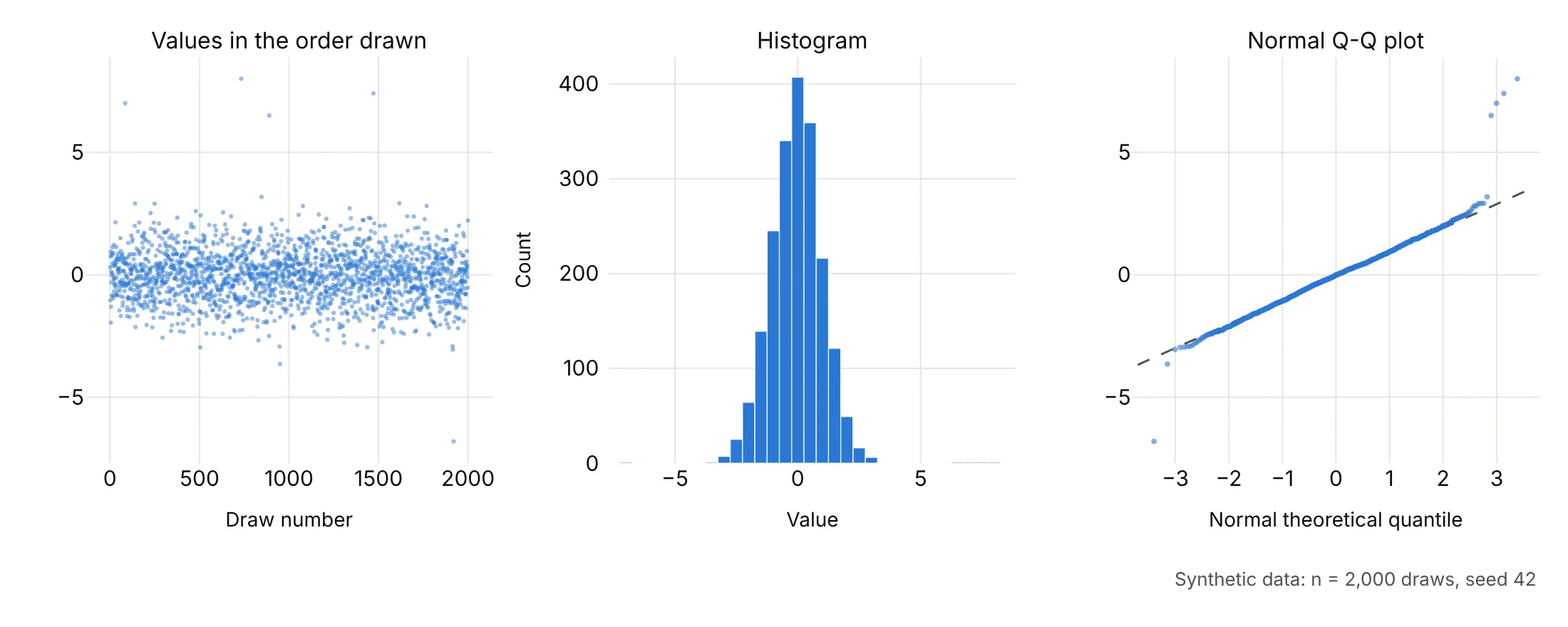
The easiest way to learn to read a Q-Q plot is to draw samples whose distribution you already know. Each row below is one synthetic sample of 2,000 random draws (seed 42), shown three ways: the values in the order they were drawn, a histogram, and a normal Q-Q plot with a dashed line through the quartiles.

Normal data lies on the straight line. If the data are a perfectly normal sample, the Q-Q plot is a straight line, apart from small wiggles in the last few points at each end, where single random values decide the position:

Synthetic normal sample of 2,000 draws shown three ways: a band of points around 0 against draw number, a bell-shaped histogram, and a normal Q-Q plot whose points lie on the dashed line from about -3 to +3

Uniform data makes an S with flat ends. A uniform sample has no tails at all, since every value falls between a hard minimum and maximum, so its ends flatten out where a normal distribution would keep going. This is what light tails look like:

Synthetic uniform sample of 2,000 draws between -1.7 and +1.7: a flat band of points, a flat histogram, and a Q-Q plot that is steep in the middle and flattens into horizontal runs at both ends

Heavy-tailed data makes an S with steep ends. A Student's t distribution with 3 degrees of freedom looks normal in the middle of the histogram, but a few draws land far out, and on the Q-Q plot the left end drops below the line and the right end rises above it. Stock and oil returns look like this:

Synthetic Student's t sample with 3 degrees of freedom: points mostly near 0 with occasional values beyond 5 and -5, a narrow peaked histogram, and a Q-Q plot that follows the line in the middle and bends away at both ends, reaching about 14 at the top

Right-skewed data bends up at the right. A log-normal sample piles up at low values and stretches out to the right, so the Q-Q plot curves upward like a hockey stick. Plotting the log of these values would give a straight line:

Synthetic log-normal sample: points crowded between 0 and 2 with a few up to 6.7, a histogram with a long right tail, and a Q-Q plot that curves up above the line at the right and flattens at the left

Two groups make a step in the middle. A mix of two normal distributions centered at -2 and +2 shows two bands in the series and two peaks in the histogram, and on the Q-Q plot two sloping runs joined by a near-vertical jump where the gap between the groups is:

Synthetic mix of two normal distributions centered at -2 and +2: two horizontal bands of points, a histogram with two peaks, and a Q-Q plot with two flatter runs joined by a steep jump at 0

Outliers sit off the line on their own. A normal sample with 5 values replaced, four of them by numbers between 6.5 and 8 and one by -6.8, stays on the line everywhere except at those points, which a histogram with 50 bins barely shows:

Synthetic normal sample with five outliers: a band of points with a few far above and one far below, a histogram where the outliers are almost invisible bars, and a Q-Q plot on the dashed line except for points at the top right near 7 and the bottom left near -7

The same shapes in real data

Real data rarely matches one of those patterns exactly, but the same shapes show up. These are four real data sets, each with a dashed line through its quartiles:

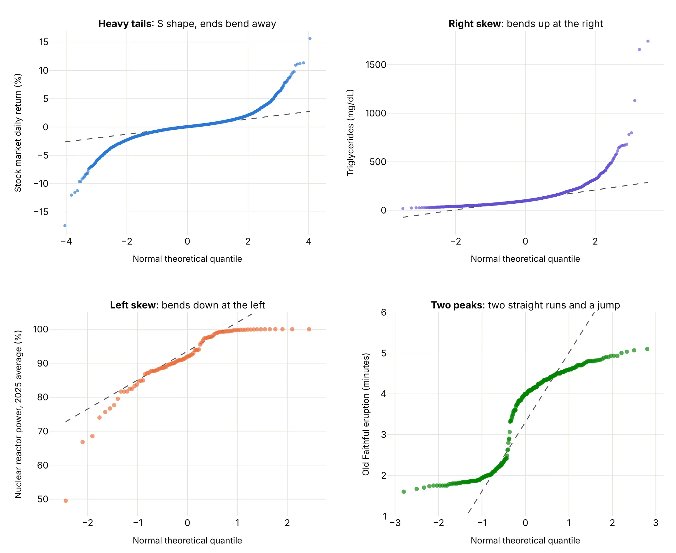
Four normal Q-Q plots: US stock returns in an S shape (heavy tails), triglycerides bending up at the right (right skew), the 2025 average power level of 94 US nuclear reactors bending down at the left and flattening at 100% (left skew), and Old Faithful eruption durations in two flat runs joined by a jump (two peaks)

Heavy tails: an S shape, with the left end below the line and the right end above it. The extreme values are more extreme than a normal distribution allows (daily stock returns).
Right skew: a curve that bends up at the right. The high values stretch out and the low values bunch up (triglycerides, flood flows, incomes). Take logs and plot again.
Left skew: a curve that bends down at the left (the 2025 average power level of 94 US nuclear reactors, where the middle half averaged 88% to 99% and the lowest 49.6%).
Two peaks: two straight runs joined by a steep jump, one for each group (Old Faithful's short and long eruptions).
Light tails look like the S shape turned the other way, with the ends flatter than the line, as in data with a hard minimum and maximum.
Steps come from rounded or whole-number data, and a few points far from the line at one end are outliers, as in Newcomb's measurements below.

A short history

Engineers and hydrologists plotted sorted measurements on printed probability paper long before computers, and Wikipedia's Q-Q plot article still lists the plotting position Allen Hazen used for river flows in 1914. Cuthbert Daniel's half-normal plots (1959) used the same idea to spot the real effects in factorial experiments, and Martin Wilk and Ram Gnanadesikan's 1968 Biometrika paper, the reference Wikipedia gives for the definition, set out probability plotting methods for comparing distributions. James Filliben's 1975 correlation test gave the plotting positions SciPy uses today. Genetics added the p-value Q-Q plot, with Devlin and Roeder's (1999) genomic control factor λ to measure inflation. We couldn't find the data behind the early examples in a public form to redraw them, so example 7 below draws flood flows on the kind of probability paper Hazen used.

Alternatives to a Q-Q plot

Here's the same century of stock market days drawn six ways. Some are better for the question, some worse, some just different:

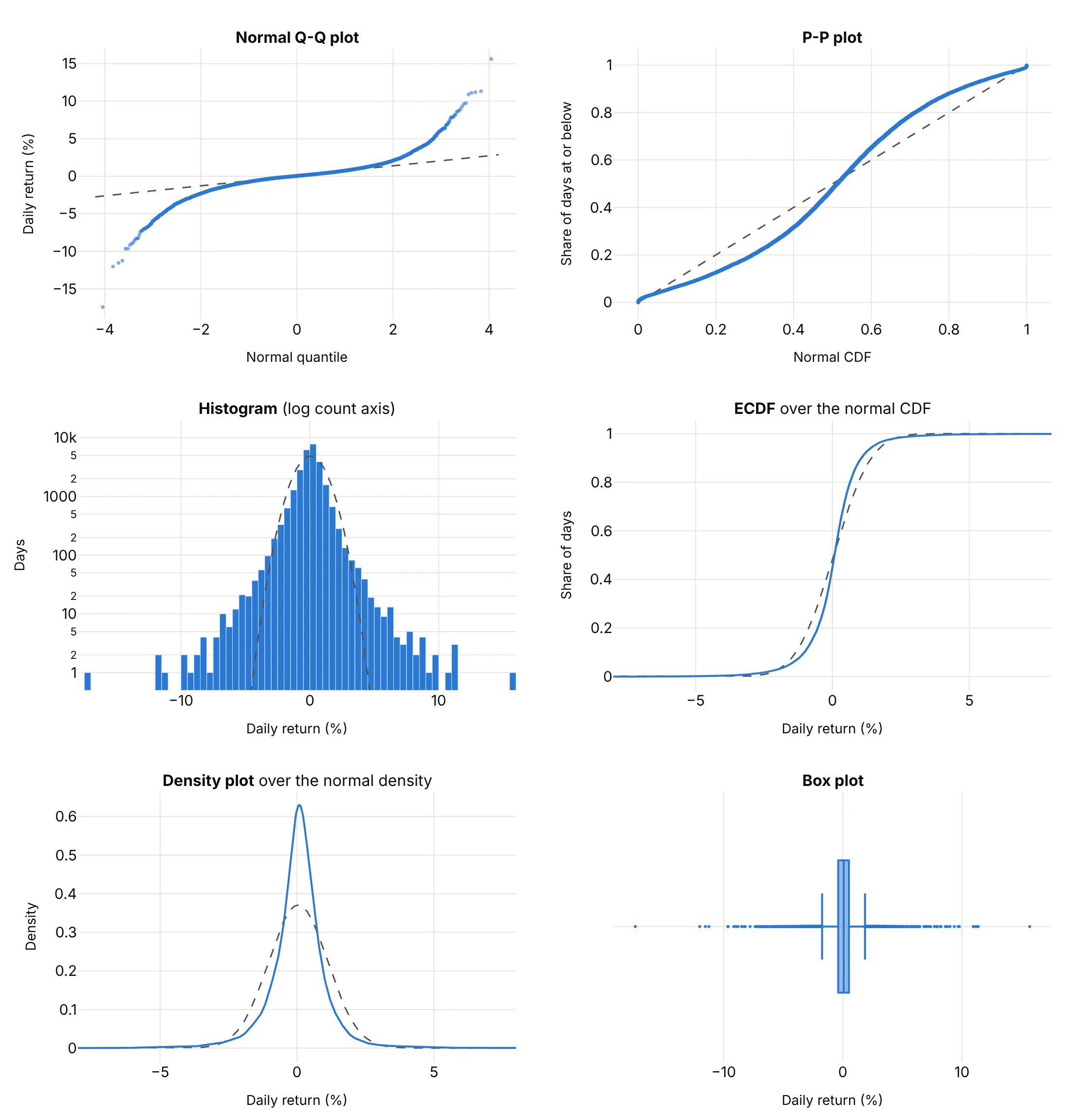
The 26,338 US stock market daily returns drawn six ways: a normal Q-Q plot with an S shape, a P-P plot that crosses its diagonal near the middle, a histogram on a log count axis with a normal curve, an ECDF over a normal CDF, a density plot with a taller narrower peak than the normal curve, and a box plot with hundreds of outlier dots

P-P plot (worse for tails, different). It plots the share of days at or below each value against the normal's share, so both axes run from 0 to 1. The middle gets most of the room and the tails are squeezed into the corners, which hides exactly what a Q-Q plot shows best.
Histogram (works too, with a log count axis). It shows the shape directly and is easier for a general audience, but the tails are a few bars of 1 or 2 days that depend on the bin width.
ECDF plot (different). Over a normal cumulative distribution function (CDF), it shows the middle is steeper than normal, but the tails hug 0% and 100% where you can't see them.
Density plot (works too, for the middle). The peak is taller and narrower than the normal curve, which is the other half of heavy tails, but the smoothing flattens the extreme days.
Box plot (worse). It flags hundreds of days as outliers without saying whether there are more than a normal distribution would have.

How to make a Q-Q plot

With AI

ChatGPT, Claude Code, GitHub Copilot, Cursor and other AI tools are excellent at writing Plotly code. Name Plotly in the prompt, and say which distribution to compare against and how to draw the reference line:

Make a plotly normal Q-Q plot from returns.csv (columns: date, ret, the daily return in percent).

- Compute the points with scipy.stats.probplot(ret, dist="norm") and draw them with go.Scattergl,
  5 px markers at 0.6 opacity, the date in the hover text.
- Add a dashed reference line through the first and third quartiles (like R's qqline), not a
  least-squares line, so the tails don't pull it.
- Label the lowest and highest days with their dates.
- Axis titles: "Normal theoretical quantile" and "Daily return (%)". A title that states the takeaway.
- Check: print how many days are 5 or more standard deviations from the mean and how many a normal
  distribution would expect.

With Plotly Studio

Plotly Studio is a desktop app where you point an AI at a dataset and it builds charts and a Dash app around your questions. Ask for a Q-Q plot the same way:

Show a normal Q-Q plot of the residuals of a regression of oil industry returns on market returns, with a dashed reference line, the days beyond 4 standard deviations in red with their dates, and a dropdown to switch between a normal and a Student's t distribution.

Make a Q-Q plot in Python or JavaScript

This is the code AI tools write under the hood. In Python, scipy.stats.probplot returns the theoretical quantiles and the sorted data, and Plotly draws them as a scatter trace with a line:

import numpy as np
import pandas as pd
import plotly.graph_objects as go
from scipy import stats

returns = pd.read_csv("returns.csv")["ret"]  # one column of daily returns in percent

(theoretical, ordered), (slope, intercept, r) = stats.probplot(returns, dist="norm")

# Reference line through the quartiles (what R's qqline draws), so the tails don't pull it
q1, q3 = np.percentile(returns, [25, 75])
z1, z3 = stats.norm.ppf([0.25, 0.75])
line_slope = (q3 - q1) / (z3 - z1)
x_line = np.array([theoretical.min(), theoretical.max()])

fig = go.Figure([
    go.Scatter(x=x_line, y=q1 + line_slope * (x_line - z1), mode="lines",
               line=dict(dash="dash", color="gray"), name="Normal"),
    go.Scattergl(x=theoretical, y=ordered, mode="markers", marker=dict(size=4, opacity=0.6), name="Days"),
])
fig.update_layout(xaxis_title="Normal theoretical quantile", yaxis_title="Daily return (%)", showlegend=False)
fig.show()

probplot also returns a least-squares line (slope, intercept) and its correlation r, which is a good one-number measure of how straight the plot is. For any other distribution, pass it as dist with its shape in sparams, such as dist="t", sparams=(3,) or dist="expon". SciPy's documentation calls this a probability plot; with the sorted data on the y axis it is the same chart other tools call a normal Q-Q plot.

To check regression residuals, statsmodels' ProbPlot gives the same points from a fitted model, and fit=True standardizes them so you can compare against the 45° line:

import pandas as pd
import plotly.graph_objects as go
import statsmodels.api as sm
import statsmodels.formula.api as smf

df = pd.read_csv("galton.csv")  # family, midparent, gender, child
model = smf.ols("child ~ midparent + gender", data=df).fit()

pp = sm.ProbPlot(model.resid, fit=True)  # fit=True standardizes the residuals
fig = go.Figure([
    go.Scatter(x=[-3.5, 3.5], y=[-3.5, 3.5], mode="lines", line=dict(dash="dash", color="gray")),
    go.Scatter(x=pp.theoretical_quantiles, y=pp.sample_quantiles, mode="markers"),
])
fig.update_layout(xaxis_title="Normal theoretical quantile", yaxis_title="Standardized residual", showlegend=False)
fig.show()

sm.qqplot draws the same thing with matplotlib; using ProbPlot and Plotly gives you hover, zoom and a chart you can put in a Dash app.

In JavaScript, plotly.js draws a Q-Q plot from a scatter trace once you've sorted the data and computed the normal quantiles:

<div id="chart"></div>
<script src="https://cdn.plot.ly/plotly-4.1.1.min.js"></script>
<script>
  // Newcomb's 66 passage times of light, 1882 (ns above 24,800), from R's MASS::newcomb
  const values = [28, -44, 29, 30, 24, 28, 37, 32, 36, 27, 26, 28, 29, 26, 27, 22, 23, 20, 25, 25, 36, 23, 31, 32, 24, 27, 33, 16,
    24, 29, 36, 21, 28, 26, 27, 27, 32, 25, 28, 24, 40, 21, 31, 32, 28, 26, 30, 27, 26, 24, 32, 29, 34, -2, 25, 19,
    36, 29, 30, 22, 28, 33, 39, 25, 16, 23];

  // Inverse of the standard normal CDF (Acklam's rational approximation, accurate to about 1e-9)
  function qnorm(p) {
    const a = [-39.6968302866538, 220.946098424521, -275.928510446969, 138.357751867269, -30.6647980661472, 2.50662827745924];
    const b = [-54.4760987982241, 161.585836858041, -155.698979859887, 66.8013118877197, -13.2806815528857];
    const c = [-0.00778489400243029, -0.322396458041136, -2.40075827716184, -2.54973253934373, 4.37466414146497, 2.93816398269878];
    const d = [0.00778469570904146, 0.32246712907004, 2.445134137143, 3.75440866190742];
    const tail = q => (((((c[0]*q + c[1])*q + c[2])*q + c[3])*q + c[4])*q + c[5]) / ((((d[0]*q + d[1])*q + d[2])*q + d[3])*q + 1);
    if (p < 0.02425) return tail(Math.sqrt(-2 * Math.log(p)));
    if (p > 0.97575) return -tail(Math.sqrt(-2 * Math.log(1 - p)));
    const q = p - 0.5, r = q * q;
    return (((((a[0]*r + a[1])*r + a[2])*r + a[3])*r + a[4])*r + a[5]) * q / (((((b[0]*r + b[1])*r + b[2])*r + b[3])*r + b[4])*r + 1);
  }

  const sorted = [...values].sort((x, y) => x - y);
  const n = sorted.length;
  const theoretical = sorted.map((_, i) => qnorm((i + 0.5) / n));  // plotting positions (i - 0.5) / n
  const quantile = p => { const h = (n - 1) * p, lo = Math.floor(h); return sorted[lo] + (h - lo) * (sorted[lo + 1] - sorted[lo]); };
  const slope = (quantile(0.75) - quantile(0.25)) / (qnorm(0.75) - qnorm(0.25));  // line through the quartiles
  const line = z => quantile(0.25) + slope * (z - qnorm(0.25));

  Plotly.newPlot("chart", [
    {x: [-2.5, 2.5], y: [line(-2.5), line(2.5)], mode: "lines", line: {dash: "dash", color: "gray"}},
    {x: theoretical, y: sorted, mode: "markers", marker: {size: 9}}
  ], {
    width: 800, height: 520, showlegend: false,
    xaxis: {title: {text: "Normal theoretical quantile"}},
    yaxis: {title: {text: "Passage time (ns above 24,800)"}}
  });
</script>

For a two-sample Q-Q plot, skip the normal quantiles: compute both samples' quantiles at the same probabilities (np.quantile(a, probs) and np.quantile(b, probs)) and plot one against the other with a y = x line.

Share it

Every Plotly chart has a Share chart button (the cloud icon in its toolbar) that uploads it to Plotly Cloud and gives you a link. Only you can see it until you change its visibility.

For a live app, put the chart in a Dash app and publish it with the Plotly Cloud command-line interface (CLI). Coding agents can run these commands for you:

pip install "dash[cloud]"
plotly user login
plotly app publish

If your data has to stay in your own cloud or data center, publish to Dash Enterprise instead.

Dos and don'ts

A Q-Q plot is only as useful as the line you judge it against, so most of the work is the reference line, the markers and the labels. Here are the stock market days both ways, in the same color.

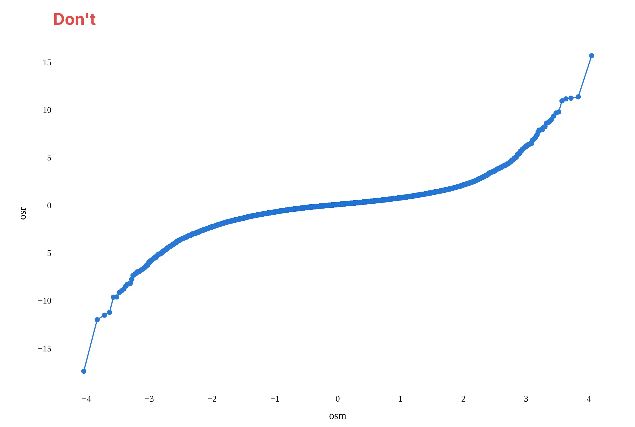
Don't join the points with a line, which makes the few tail days look like a continuous curve, leave out the reference line, keep probplot's raw names osm and osr as axis titles, or use a default serif font:

The stock market Q-Q plot with every point joined by a line, no reference line, the axis titles osm and osr, a serif font and large markers that merge into a thick band

Do draw markers only, small and partly transparent so the dense middle doesn't hide the tails, add a dashed reference line through the quartiles, write axis titles in words with units, and label the extreme points:

The same Q-Q plot with small transparent markers, a dashed line labeled "Normal through the quartiles", axis titles "Normal theoretical quantile" and "Daily return (%)", and the days October 19, 1987 and March 15, 1933 labeled

Checklist

Say which distribution is on the x axis ("Normal theoretical quantile", "Expected −log10 p").
Draw a reference line and say what it is: through the quartiles for raw data, y = x for standardized residuals, two samples or p-values.
Use WebGL (go.Scattergl) above about 10,000 points.
Label the extreme points with what they are (a date, a gene, a sample ID).
For p-values, add the 95% band and the genomic control λ.
Take logs and plot again when the data are right-skewed and positive.

Don't

Fit the reference line by least squares to heavy-tailed data and then say the tails look fine; the tails pull the line toward them.
Read wiggles in the last few points of a small sample as a pattern. With 30 points, the ends wander even for normal data.
Use a Q-Q plot alone to show a general audience the shape of a distribution; pair it with a histogram.

Options to customize

A Q-Q plot in Plotly is a scatter trace of computed quantiles plus a line, so these are the options that matter most. The full lists are in the scatter trace reference, the scattergl trace reference and the SciPy probplot documentation.

scipy.stats.probplot(x, dist=..., sparams=...): theoretical quantiles and sorted data for any SciPy distribution, plus a least-squares line and its correlation r.
statsmodels.api.ProbPlot(x, dist=..., fit=True): the same points from residuals or data, standardized with fit=True; qqplot_2samples compares two samples.
go.Scattergl or render_mode="webgl": WebGL markers for tens of thousands of points or more.
marker.size, marker.opacity: 4 to 6 px at 0.5 to 0.7 opacity for big samples, so the middle stays light and the tails stand out.
mode="lines" trace or fig.add_shape(type="line"): the reference line, with line_dash="dash".
customdata and hovertemplate: the date, ID or label of each sorted point, so hovering a tail point tells you which day or sample it is.
add_annotation with ax, ay: labels with leader lines on the extreme points.
xaxis.tickvals and ticktext: probability paper, with return periods or percentages at the normal quantiles.
xaxis.type="log", yaxis.type="log": log axes for waiting times and other positive data that span decades.
yaxis.scaleanchor="x": equal scales, so a 45° line looks like 45° when both axes share units.
fill="tonexty": a shaded confidence band from two line traces, as in the GWAS example.
make_subplots with shared_yaxes=True: the same data against two candidate distributions, side by side.

More Q-Q plot examples

Seven more Q-Q plots built from real public data, each with its source, the technique that makes it work and a prompt to rebuild it.

1. Newcomb's 1882 speed of light measurements

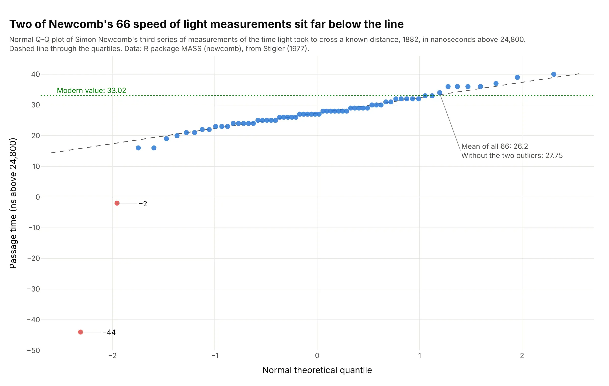
Normal Q-Q plot of Simon Newcomb's 66 measurements of the passage time of light in 1882: 64 points along a dashed line from 16 to 40, two red outliers far below at -2 and -44, and a dotted green line at the modern value of 33.02

Two of Newcomb's 66 measurements, -44 and -2, sit far below the line, while the other 64 follow it from 16 to 40. They pull the mean from 27.75 down to 26.2. Data: Newcomb's third series, R package MASS (newcomb), from Stigler (1977).

Tip: draw the reference line through the quartiles, so a couple of outliers can't tilt it.

Get the data from the R package MASS data set newcomb (Simon Newcomb's 1882 third series of 66
passage times of light, in nanoseconds above 24,800; Stigler 1977, Table 5), as a table (columns: value).

Build a plotly normal Q-Q plot with scipy.stats.probplot, a dashed line through the quartiles, the two
negative values in red and labeled, and a dotted line at the modern value of 33.02.

2. Brent crude oil against a normal and a Student's t distribution

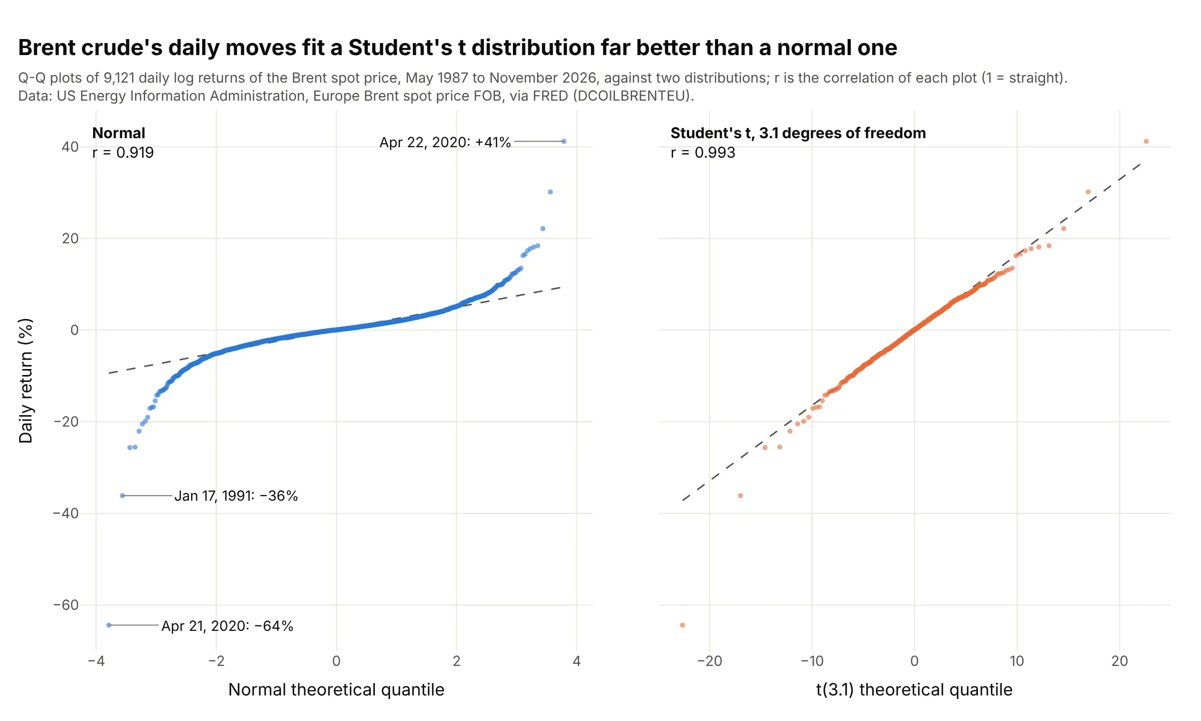
Two Q-Q plots of 9,121 daily Brent crude returns from 1987 to 2026: against a normal distribution the points form a steep S with r = 0.919 and April 21, 2020 at -64%; against a Student's t with 3.1 degrees of freedom they lie along a straight line with r = 0.993

Against a normal distribution, Brent's daily returns form a steep S (r = 0.919); against a Student's t with 3.1 degrees of freedom they lie close to a straight line (r = 0.993). The worst day, April 21, 2020, fell 64%. Data: US Energy Information Administration, Brent spot price via Federal Reserve Economic Data (FRED).

Tip: fit the candidate distribution with scipy.stats.t.fit and pass its shape to probplot as sparams.

Get the data from FRED series DCOILBRENTEU (US Energy Information Administration, Europe Brent spot price free on board, daily, dollars per barrel)
and compute daily log returns in percent (columns: date, price, ret).

Build two plotly Q-Q plots side by side with shared y: ret against a normal distribution and against a
Student's t fitted with scipy.stats.t.fit, each with probplot's least-squares line and its r in the corner,
and the three largest moves labeled with their dates.

3. Triglycerides before and after a log transform

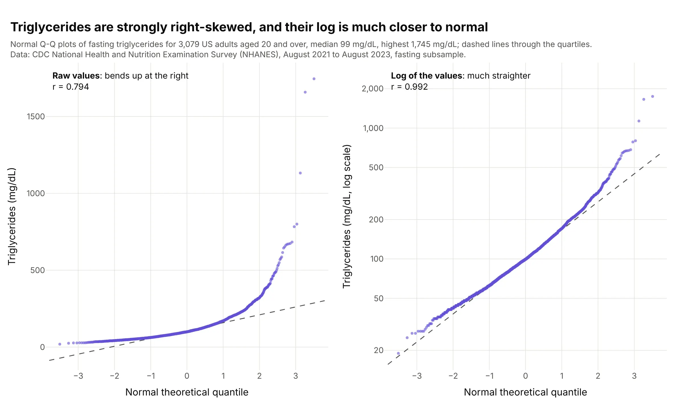
Two normal Q-Q plots of fasting triglycerides for 3,079 US adults: the raw values bend sharply upward at the right with r = 0.794 and a maximum of 1,745 mg/dL; on a log scale the points are much straighter, r = 0.992

Fasting triglycerides in 3,079 US adults bend sharply upward on a normal Q-Q plot (r = 0.794), with a median of 99 mg/dL and a maximum of 1,745. Their logs are much straighter (r = 0.992), which is why lab values like these are usually analyzed on a log scale. Data: CDC NHANES August 2021 to August 2023, fasting subsample.

Tip: plot the log on a y axis labeled in the original units (20, 50, 100, 200 mg/dL), so readers don't have to convert.

Get the data from CDC NHANES August 2021-August 2023 files TRIGLY_L (LBXTLG, fasting triglycerides
mg/dL) and DEMO_L (RIDAGEYR), adults 20 and over (columns: seqn, age, trig_mg_dl).

Build two plotly normal Q-Q plots side by side: the raw values and log10 of them, each with a dashed
line through the quartiles and probplot's r in the corner, the log panel's y ticks labeled in mg/dL.

4. Residuals of a market model for oil stocks

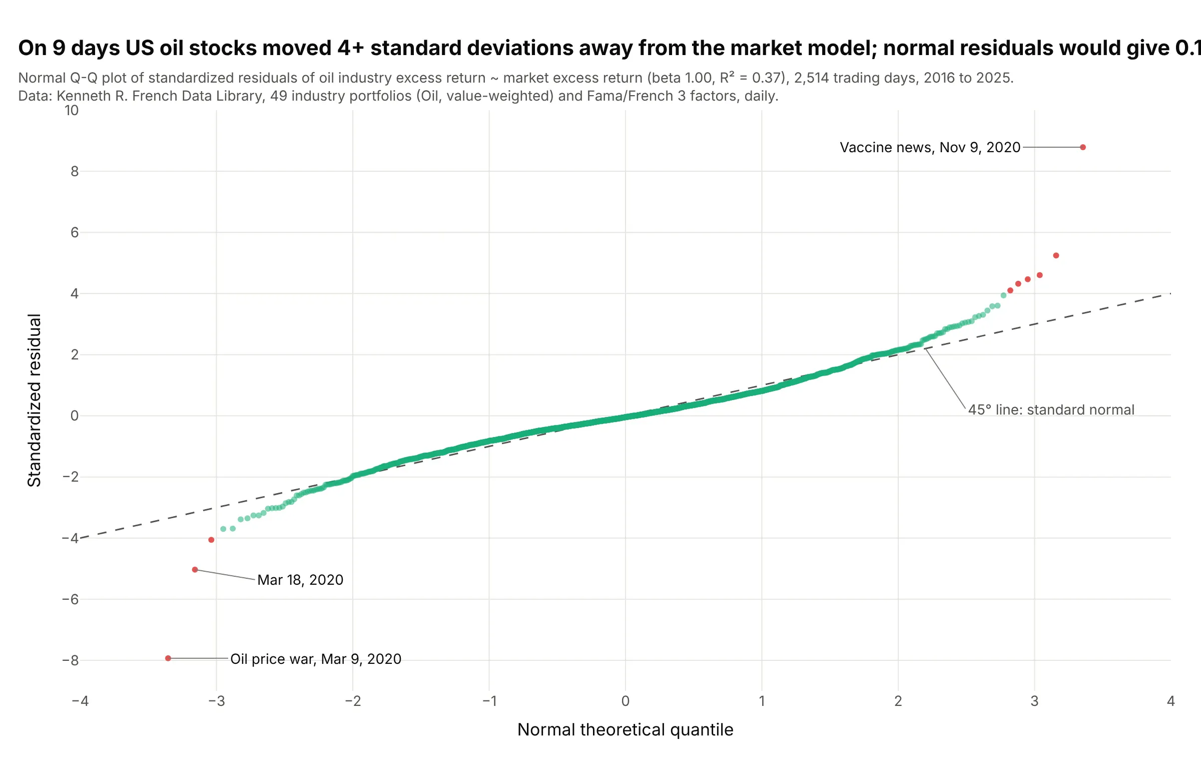
Normal Q-Q plot of the standardized residuals of a regression of US oil industry returns on market returns, 2016 to 2025: points follow the 45-degree line in the middle, with 9 red days beyond 4 standard deviations, including March 9, 2020 near -8 and November 9, 2020 near +9

On 9 of 2,514 days from 2016 to 2025, US oil stocks moved at least 4 standard deviations away from what the market predicted, where normal residuals would give 0.16. The two largest were March 9, 2020, when oil prices collapsed, and November 9, 2020, the day of the first COVID-19 vaccine results. Data: Kenneth R. French Data Library, 49 industry portfolios (Oil) and Fama/French factors, daily.

Tip: standardize the residuals (ProbPlot(resid, fit=True)) and compare them with the 45° line, so "4 standard deviations" can be read off the y axis.

Get the data from the Kenneth R. French Data Library: 49 Industry Portfolios [Daily] (value-weighted Oil)
and Fama/French 3 Factors [Daily], 2016-2025 (columns: date, oil, mkt_rf, rf).

Fit oil - rf ~ mkt_rf with statsmodels ordinary least squares and build a plotly normal Q-Q plot of the standardized
residuals from sm.ProbPlot, the 45-degree line dashed, days beyond 4 standard deviations in red with their dates on hover,
and the title giving how many days are beyond 4 standard deviations against how many a normal model expects.

5. Gaps between large earthquakes against an exponential distribution

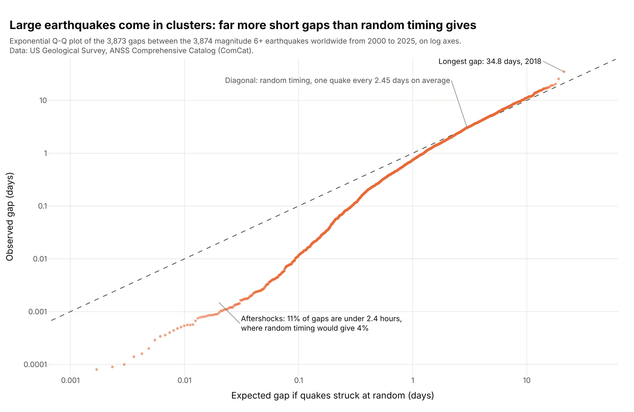
Exponential Q-Q plot on log axes of the 3,873 gaps between magnitude 6+ earthquakes from 2000 to 2025: points follow the diagonal above about 1 day and fall far below it for short gaps, with 11% of gaps under 2.4 hours where random timing would give 4%

If large earthquakes struck at random times, the gaps between them would follow an exponential distribution and sit on the diagonal. Above about a day they do, but 11% of the 3,873 gaps from 2000 to 2025 are under 2.4 hours, where random timing gives 4%, because large quakes trigger others. Data: US Geological Survey Comprehensive Catalog (ComCat), magnitude 6 and above.

Tip: use log axes for waiting times, or every gap under a day piles up in one corner.

Get the data from the US Geological Survey (USGS) earthquake catalog web service (ComCat, the Comprehensive Catalog), all earthquakes of magnitude 6 and above
from 2000-01-01 to 2025-12-31, sorted by time, and compute the gap in days to the previous one
(columns: time, mag, place, gap_days).

Build a plotly exponential Q-Q plot: probplot(gaps, dist="expon") times the mean gap on x, the sorted
gaps on y, both axes log, a dashed y = x line, and the share of gaps under 0.1 day against the exponential's.

6. Singers' heights, the classic two-sample Q-Q plot

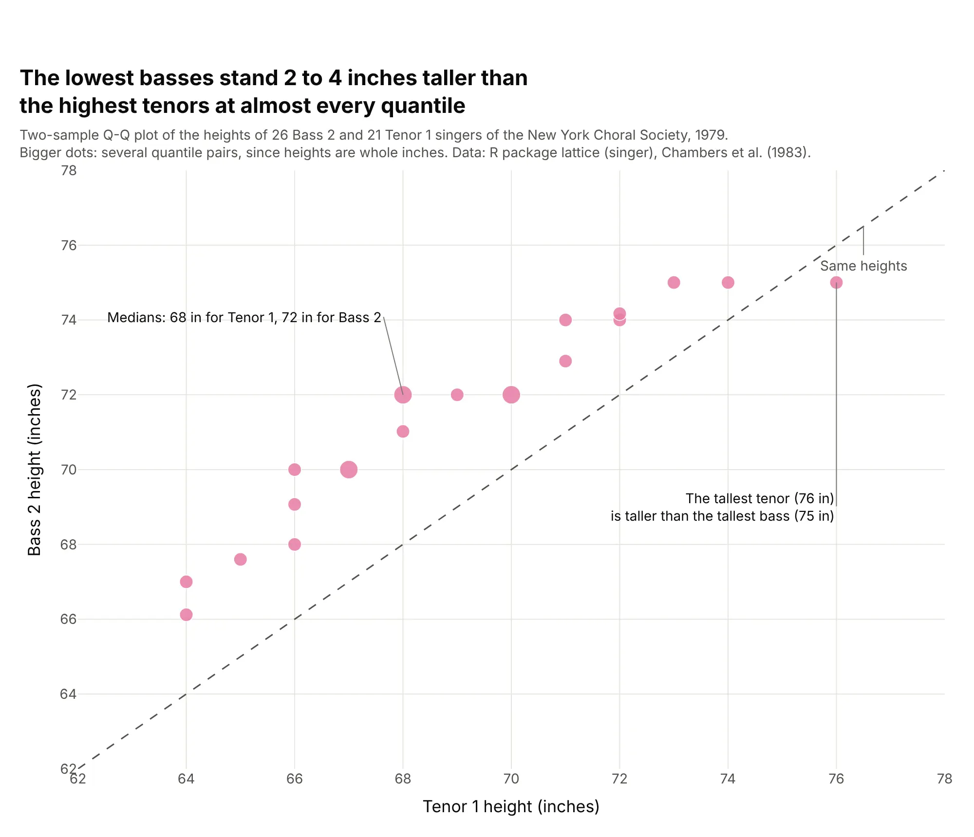
Two-sample Q-Q plot of the heights of 26 Bass 2 and 21 Tenor 1 singers of the New York Choral Society: points sit 2 to 4 inches above the dashed diagonal, with medians of 68 and 72 inches, except the top quantile where the tallest tenor at 76 inches is taller than the tallest bass at 75

At 19 of 21 quantiles the lowest basses of the New York Choral Society are 1.9 to 4 inches taller than the highest tenors, and only the tallest tenor (76 inches) beats the tallest bass. The samples don't need the same size: 26 basses against 21 tenors. Data: R package lattice (singer), from Chambers, Cleveland, Kleiner and Tukey (1983), Graphical Methods for Data Analysis.

Tip: with whole-number data, many quantile pairs land on the same spot, so size the markers by how many share it.

Get the data from the R package lattice data set singer (heights in inches of 235 New York Choral
Society singers in 1979, by voice part; Chambers et al. 1983) (columns: height, voice_part).

Build a plotly two-sample Q-Q plot of Bass 2 against Tenor 1: quantiles of both at (i - 0.5)/21 with
np.quantile, a dashed y = x line, markers sized by how many quantile pairs share a point, and the medians labeled.

7. Potomac River floods on probability paper

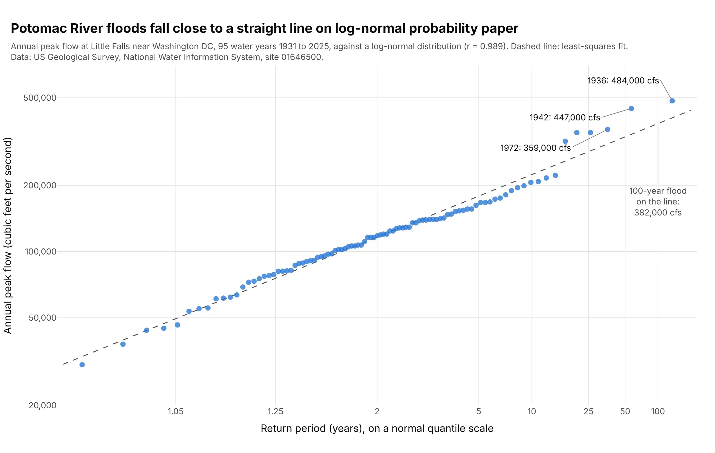
Probability plot of 95 annual peak flows of the Potomac River near Washington DC from 1931 to 2025, on a log y axis against a normal quantile x axis labeled in return periods from 1.05 to 100 years: the points follow a dashed line (r = 0.989), with the 1936 flood at 484,000 cubic feet per second and 1942 at 447,000 above it, and the line at 382,000 at 100 years

The Potomac's 95 annual peak flows fall close to a straight line on log-normal probability paper (r = 0.989, against 0.953 for a Gumbel distribution), and the line puts the 100-year flood at 382,000 cubic feet per second. The 1936 and 1942 floods sit above it at 484,000 and 447,000. Data: US Geological Survey annual peak streamflow, site 01646500.

Tip: label the x axis in return periods at the normal quantiles of 1 - 1/T, so engineers can read a 100-year flood off the line.

Get the data from the USGS National Water Information System annual peak streamflow for site 01646500 (Potomac River near Washington DC,
Little Falls pump station) as tab-separated text (columns: water_year, peak_date, peak_cfs).

Build a plotly probability plot: probplot(log10(peak_cfs), dist="norm") with the y axis as a log axis
in cfs, x ticks at norm.ppf(1 - 1/T) labeled T = 1.05, 1.25, 2, 5, 10, 25, 50, 100 years, probplot's
least-squares line dashed, the three largest floods labeled, and the line's 100-year value annotated.