Volcano Plots - A Complete Guide

TL;DR

• A volcano plot is a scatter plot of thousands of statistical tests at once, one dot per gene, protein or variant: the size of the change on the x axis (usually log2 fold change) and the strength of the evidence on the y axis (−log10 p-value).
• Volcano plots are similar to MA plots, which put mean expression on the x axis instead of the p-value, and Manhattan plots, which put genome position on it.
• The dots that matter sit in the top left and top right corners, past two thresholds that every published volcano should state on the chart: a fold change (often 2-fold) and an adjusted p-value (often q < 0.05).
• They are the standard differential expression plot for RNA-seq and proteomics, and they also summarize drug screens, GWAS results and adverse events in clinical trials.
• You can make a volcano plot with Plotly in Python from px.scatter with three dashed threshold lines, or with Dash Bio's VolcanoPlot, which draws the lines and highlights the hits for you.

What is a volcano plot?

Volcano plots look like this:

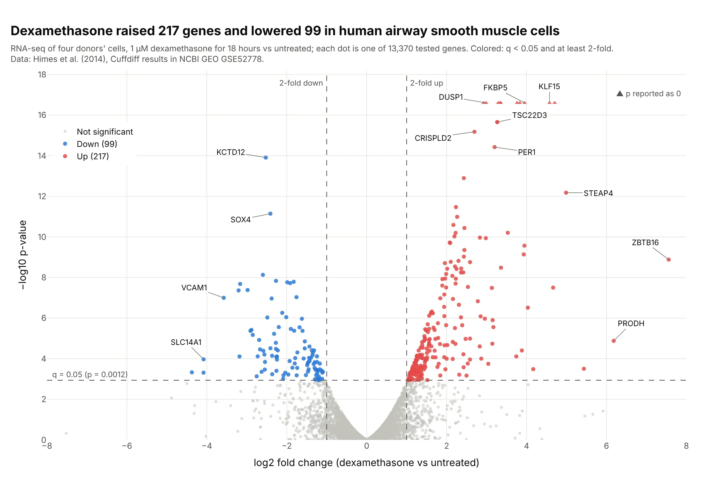
Data: Himes et al. (2014), Cuffdiff results deposited in NCBI GEO, series GSE52778.

How do you read a volcano plot? In the example above, notice these things:

• Each dot is one gene, tested for a difference between airway smooth muscle cells treated with the steroid dexamethasone and untreated cells from the same four donors.
• The x axis is the log2 fold change, so 0 means no change, +1 means twice as much and −1 means half as much. Genes that went up are on the right, like FKBP5 at +3.95 (15.5 times as much), and genes that went down are on the left, like KCTD12.
• The y axis is −log10 of the p-value, so higher means stronger evidence. The dashed horizontal line is where the adjusted p-value (q) reaches 0.05, at p = 0.0012, so every dot above it passes after correcting for 13,370 tests.
• Only the dots past both dashed lines count as hits, colored red (217 up) and blue (99 down). The gray cloud near 0 is the thousands of genes that didn't change, which gives the chart its volcano shape.
• Watch the edges. The triangles at the top are 10 genes whose p-value the software reported as exactly 0, so their height is a cap rather than a value, and ZBTB16 far right went from almost no expression to some, which makes its fold change large.

It's often used for charts like these:

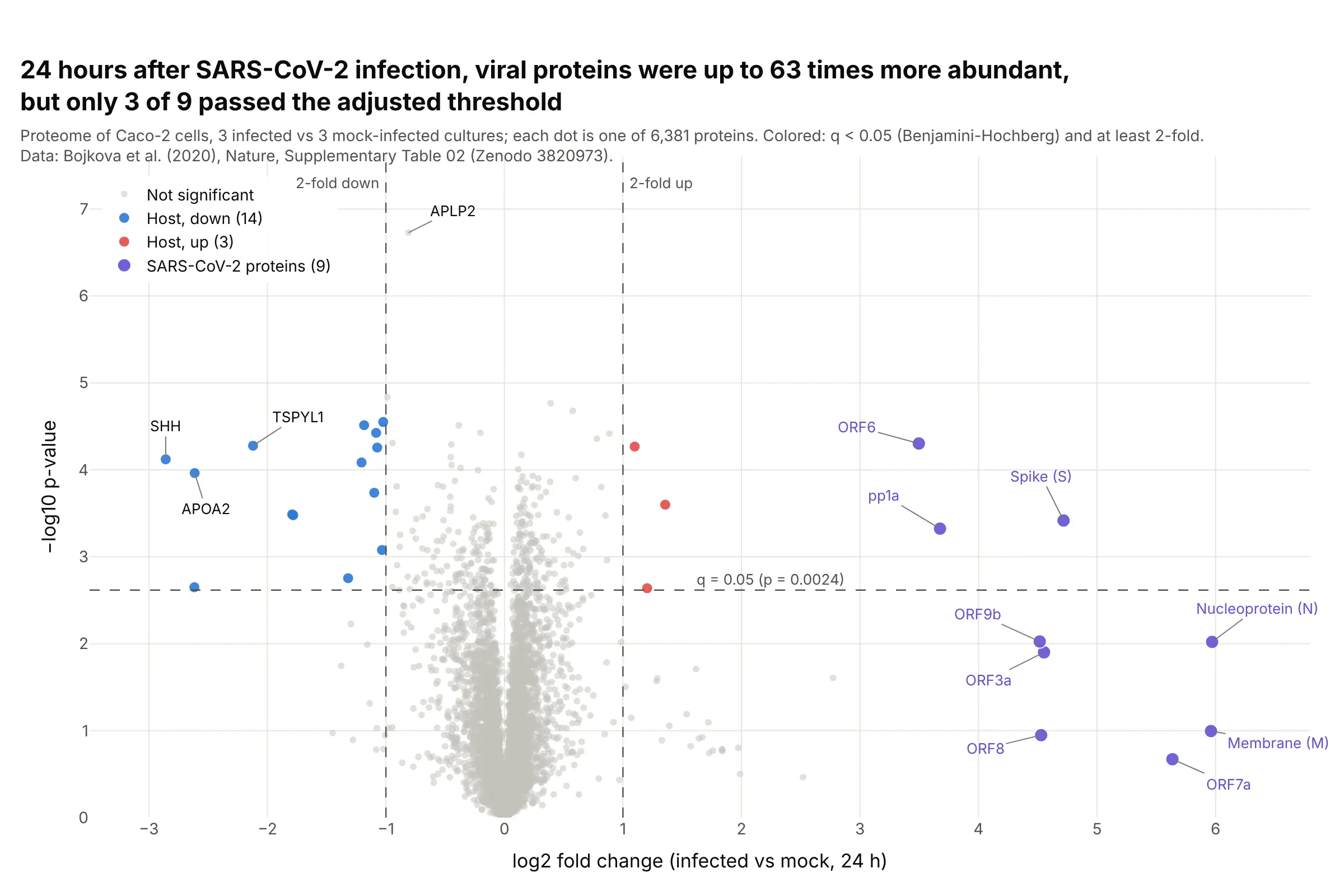
Proteomics. 24 hours after SARS-CoV-2 infection, the nucleoprotein was 63 times more abundant than in mock-infected cells, yet only 3 of the 9 viral proteins passed q < 0.05, because three replicates per group give noisy p-values. Data: Bojkova et al. (2020), Nature, Supplementary Table 02 on Zenodo.

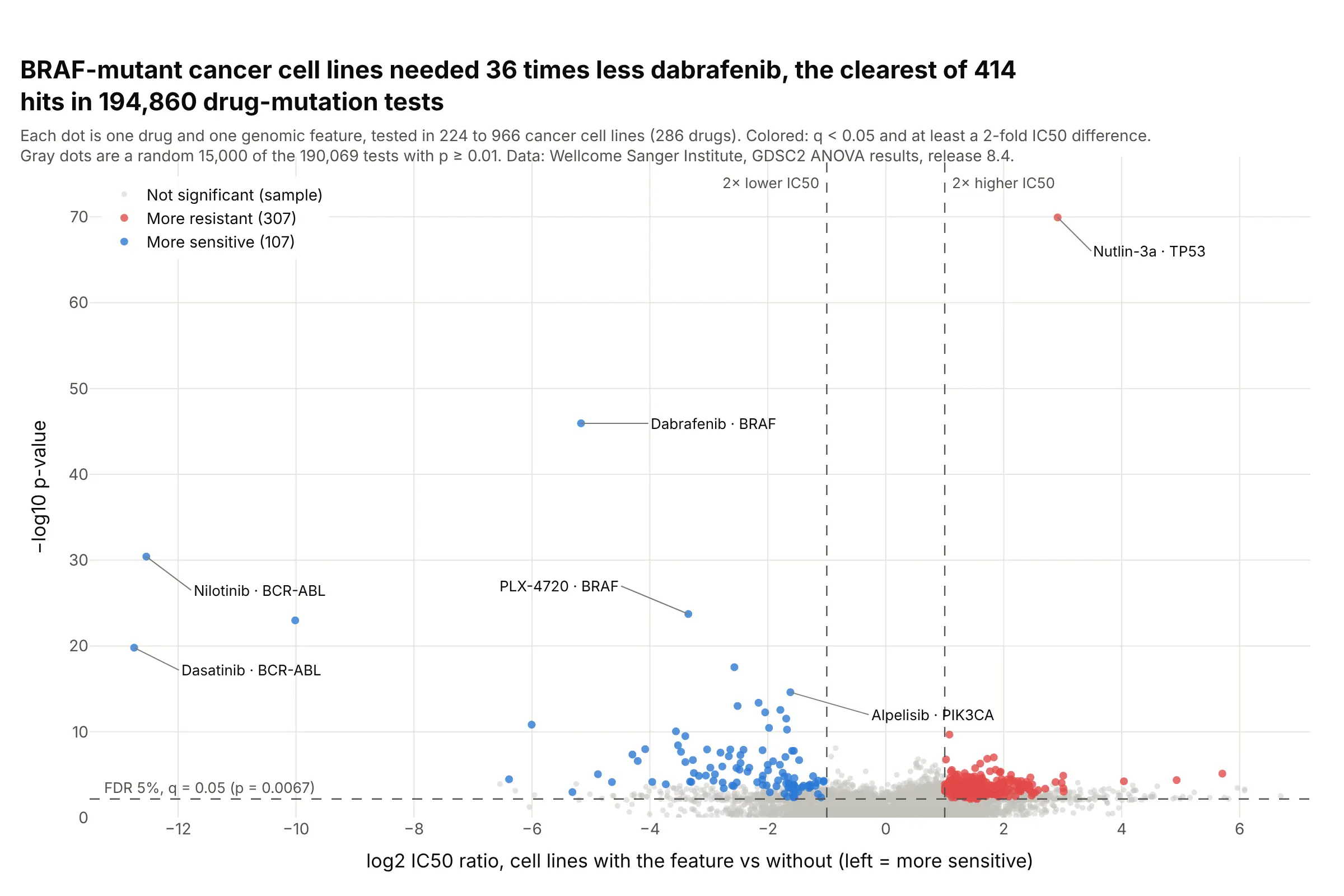
Drug screens. Across 194,860 drug and mutation tests in the GDSC cancer cell line screen, BRAF-mutant lines needed 36 times less dabrafenib than other lines, one of 414 hits past both thresholds. Data: Wellcome Sanger Institute, GDSC2 ANOVA results, release 8.4 (Iorio et al. 2016).

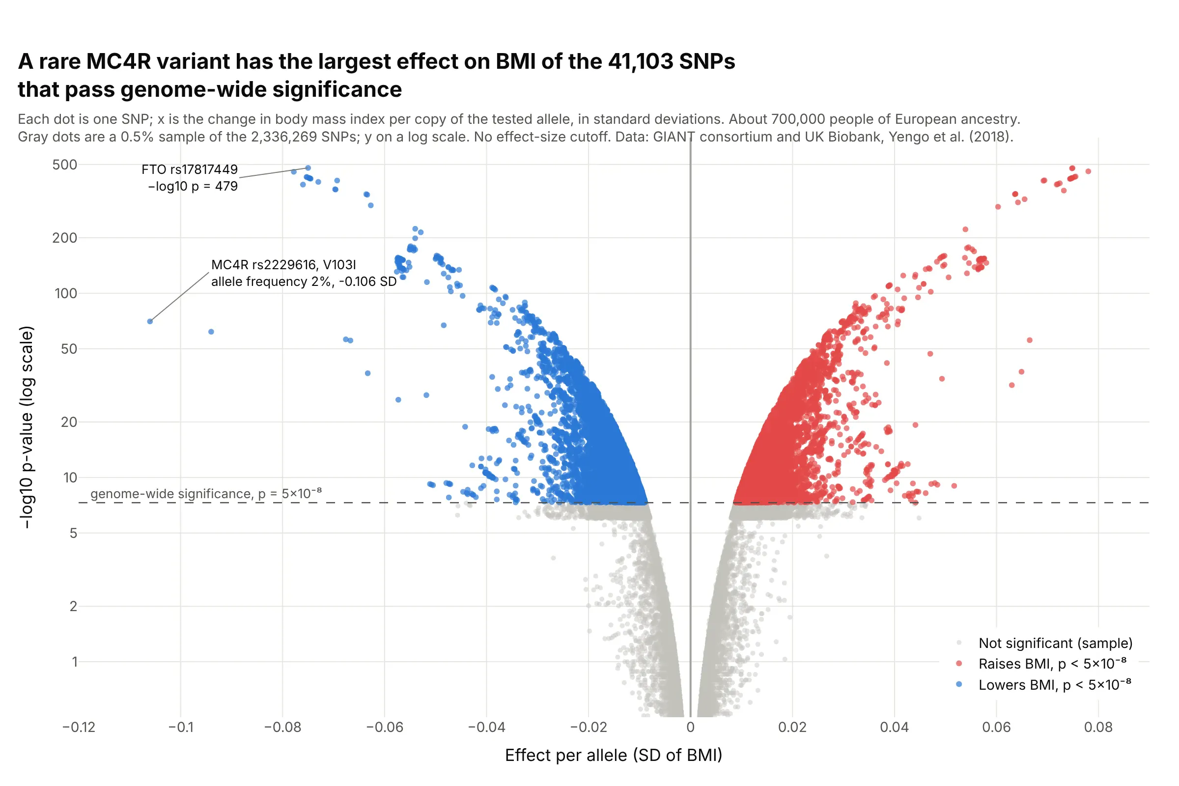
Genetic association studies. In a GWAS of about 700,000 people, a rare MC4R variant carried on 2% of chromosomes had the largest effect on BMI of the 41,103 genome-wide significant SNPs, while common FTO variants had the smallest p-values. Data: GIANT consortium and UK Biobank, Yengo et al. (2018).

A short history

Volcano plots came out of the microarray era, when a single experiment produced a fold change and a t-test for thousands of genes. Wikipedia's volcano plot article cites Jin et al. (2001) and Cui and Churchill (2003), who described "the 'volcano plot'" as "an effective and easy-to-interpret graph that summarizes both fold-change and t-test criteria". Their figure plotted −log10 p against log2 fold change with threshold bars, the same layout used today. We couldn't find their data in a public form to redraw it, so example 6 below draws the same kind of chart on Golub's 1999 leukemia microarrays. The chart later moved to RNA-seq, proteomics, genetic association studies and clinical safety tables (Zink et al. 2013).

Alternatives to a volcano plot

Here's the same airway data drawn five ways. Some are better for the question, some worse, some just different:

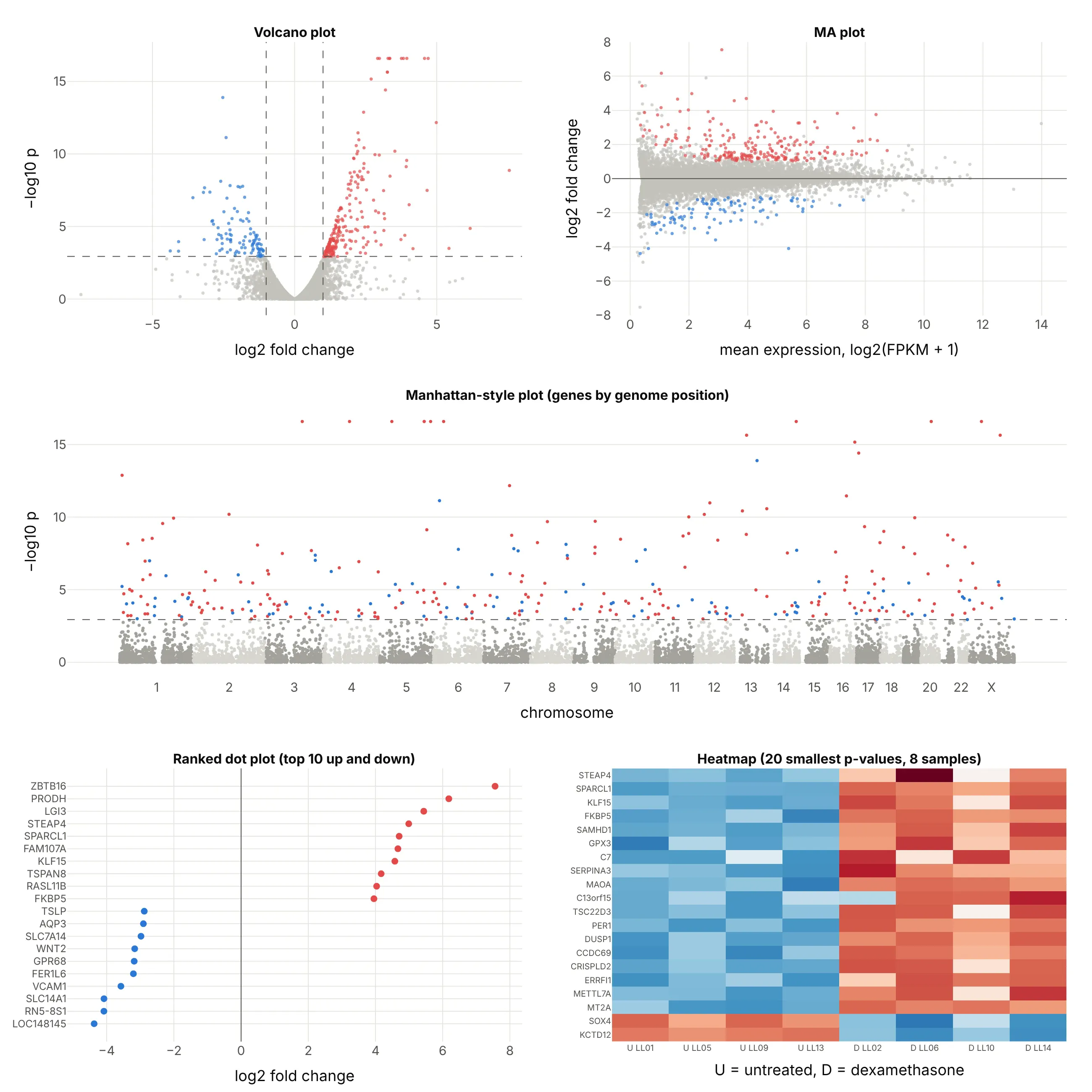
• MA plot (different, better for checking normalization). Log fold change on y against mean expression on x shows whether low-count genes swing more than high-count ones, which a volcano hides, but you can't see the p-values. DESeq2's plotMA draws this one.
• Manhattan-style plot (different). P-values by genome position show whether hits cluster on a chromosome. It is the standard chart for GWAS, shown below, but for gene expression the position rarely matters.
• Ranked dot plot (better for a short list). The 10 largest increases and decreases with their names are easier to read in a slide, but the other 13,000 genes and the evidence are gone.
• Heatmap (works too, for the top hits). Each sample's values show whether the change holds in every sample, which a volcano can't show, but it only fits a few dozen genes.
• Table sorted by p-value (worse for exploring). It's exact, but it hides the shape of the result: how many genes moved, in which direction and by how much.

The Manhattan plot is the volcano plot's closest relative in genetics. It draws every SNP at its position in the genome, so each associated region rises as a tower:

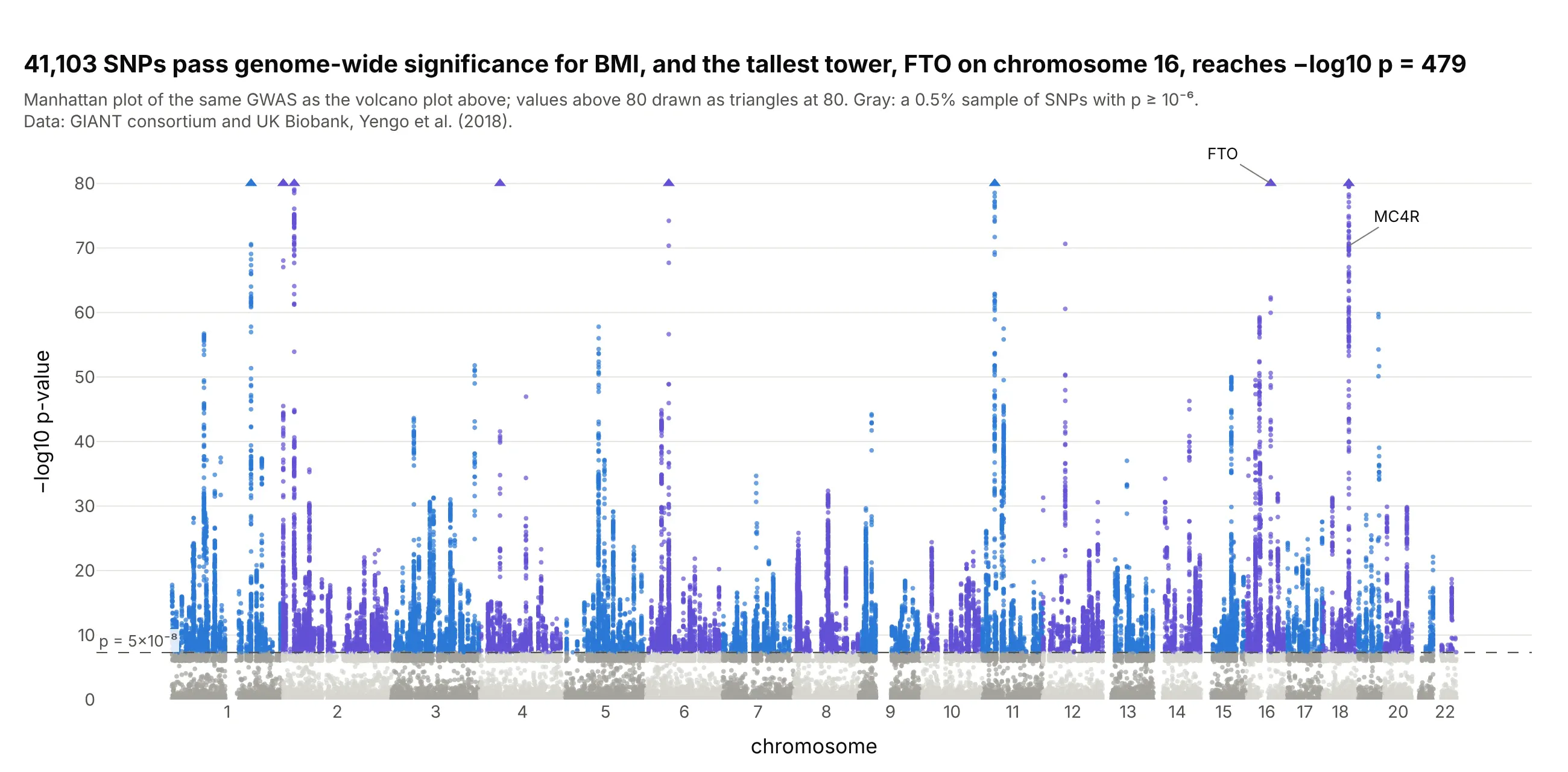
Data: GIANT consortium and UK Biobank, Yengo et al. (2018); the same results as the GWAS volcano above.

How to make a volcano plot

With AI

ChatGPT, Claude Code, GitHub Copilot, Cursor and other AI tools are excellent at writing Plotly code. Name Plotly in the prompt, and give it your thresholds so they end up on the chart:

With Plotly Studio

Plotly Studio is a desktop app where you point an AI at a dataset and it builds charts and a Dash app around your questions. Ask for a volcano plot the same way:

Show a volcano plot of the DESeq2 results with log2 fold change on x and −log10 p-value on y, hits at padj below 0.05 and at least 2-fold in red and blue, dashed threshold lines, and sliders to change both thresholds.

Make a volcano plot in Python or JavaScript

This is the code AI tools write under the hood. In Python, a volcano plot is px.scatter with a status column for the colors and three dashed lines. It takes the columns that DESeq2 and PyDESeq2 write, so it works on an RNA-seq result as it is:

The horizontal line sits at the largest p-value whose adjusted p-value is below 0.05, so the dots above it are exactly the ones that pass. If you'd rather put the adjusted p-value on the y axis, use -np.log10(df.padj) and draw the line at -np.log10(0.05). The Plotly scatter plot documentation covers hover text and styling.

In JavaScript, plotly.js draws the same thing from a scatter trace and three line shapes:

Make a volcano plot with Dash Bio

Dash Bio is Plotly's open-source library of bioinformatics charts for Dash, and its VolcanoPlot returns a Plotly figure with the threshold lines drawn and the hits highlighted. Its defaults come from genetics: effect_size_line=[-1, 1] and genomewideline_value=-log10(5e-8), given on the −log10 scale. For an RNA-seq result, set the line to your own cut:

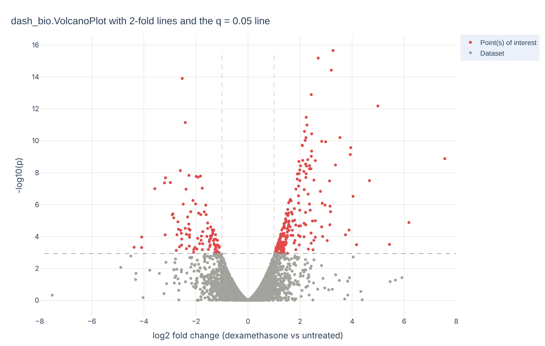
In a Dash app, put the figure in a dcc.Graph and connect a dcc.RangeSlider to effect_size_line with a callback, as the Dash Bio example does, so readers can move the fold change threshold and watch the hits change.

Share it

Every Plotly chart has a Share chart button (the cloud icon in its toolbar) that uploads it to Plotly Cloud and gives you a link. Only you can see it until you change its visibility.

For a live app, put the chart in a Dash app and publish it with the Plotly Cloud CLI. Coding agents can run these commands for you:

If your data has to stay in your own cloud or data center, publish to Dash Enterprise instead.

Dos and don'ts

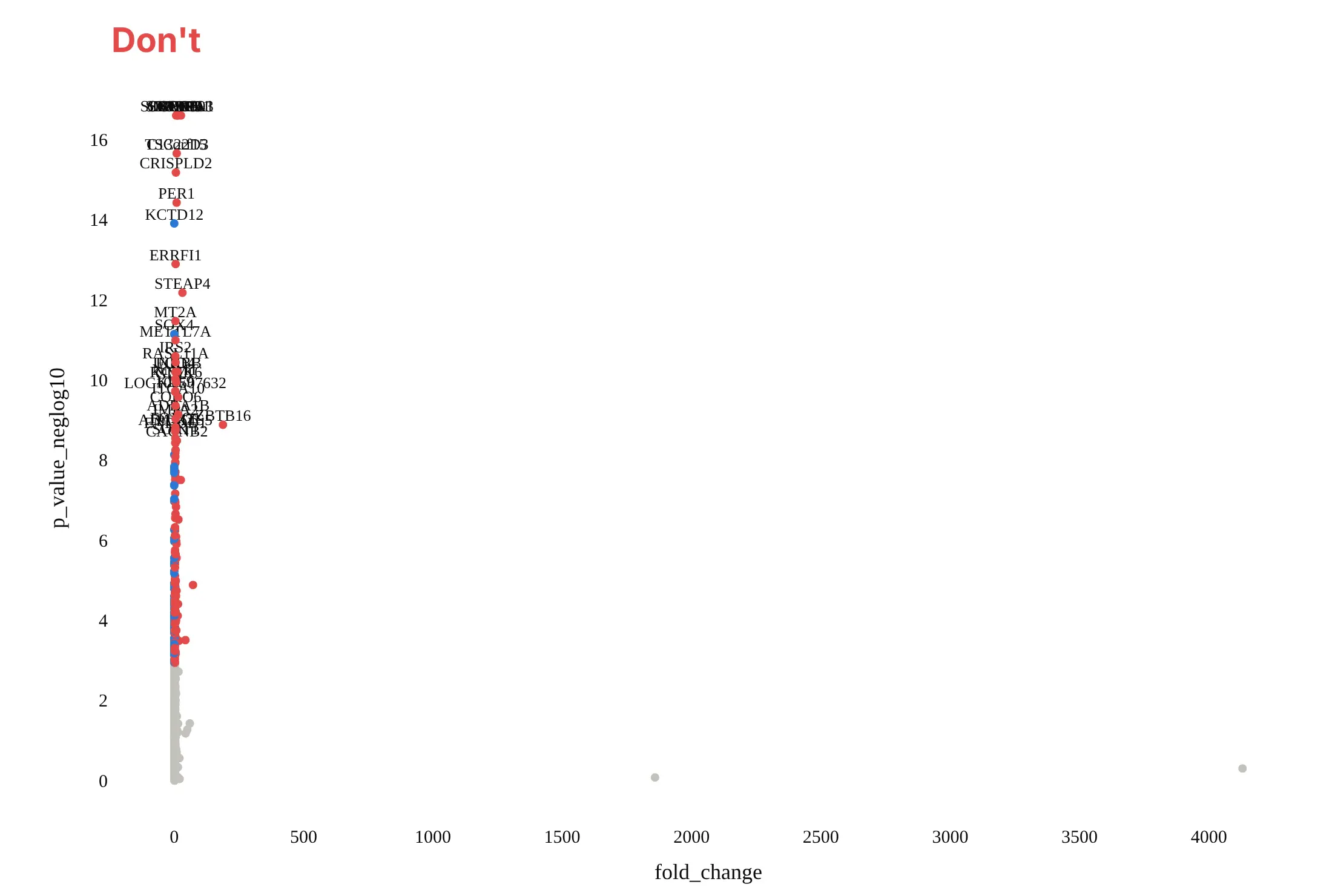
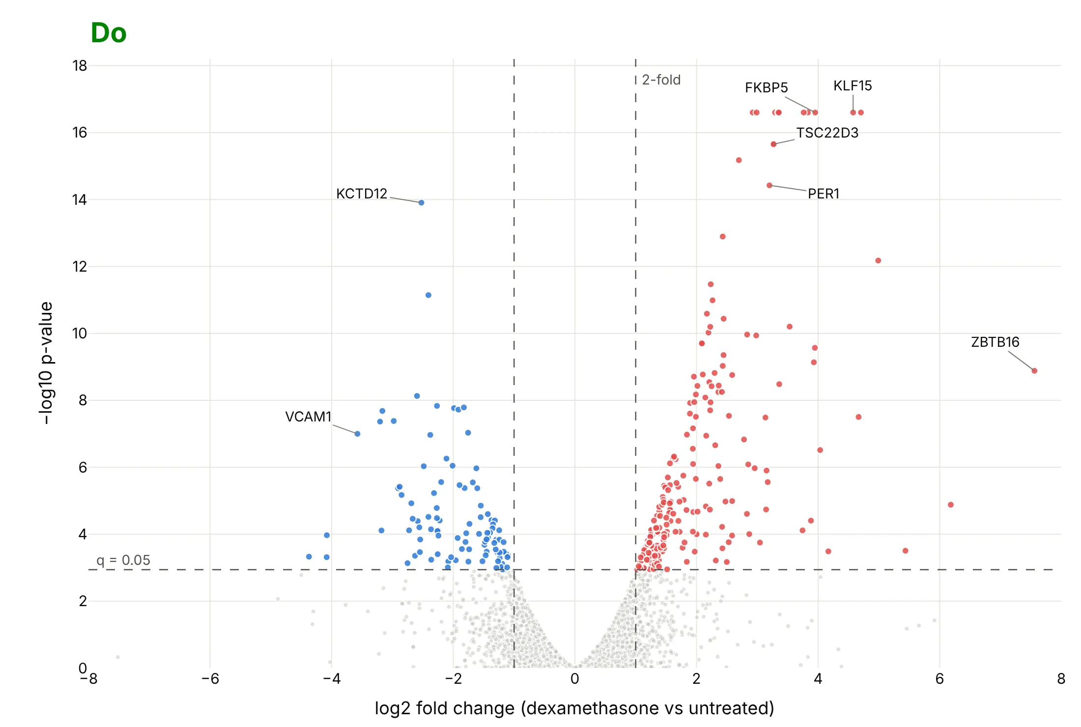
Most of the work in a published volcano plot is choosing the axes, showing the thresholds and labeling only a few points. Here are the airway results both ways, in the same colors.

Don't plot the fold change on a linear scale, which squeezes every gene that went down between 0 and 1 and lets two outliers stretch the axis to 4,130, leave out the threshold lines, label 40 genes on top of each other, or use a default serif font and raw column names as axis titles:

Do use log2 fold change so ups and downs are symmetric around 0, draw both thresholds as dashed lines with their values, make the genes that miss small and light, label a handful of genes with leader lines, and write axis titles in words:

Checklist

Do

• Put log2 fold change on x and −log10 p-value (or adjusted p-value) on y.
• State both thresholds on the chart: the fold change and the adjusted p-value, with their values.
• Color only the dots past both thresholds, with up and down in two colors that work for color-blind readers (red and blue, not red and green).
• Label 5 to 15 dots with leader lines, and put every name in the hover text.
• Say in the subtitle what was compared, how many tests there were and how p-values were adjusted.
• Mark capped values: p-values reported as 0 and fold changes from a zero count.

Don't

• Use unadjusted p < 0.05 as the threshold for thousands of tests.
• Read a dot's height as effect size, or its distance from 0 as evidence.
• Let a few extreme fold changes set the axis range for the whole chart.

Options to customize

A volcano plot in Plotly is px.scatter (or go.Scattergl) plus lines and annotations, so these are the options that matter most. The full lists are in the px.scatter reference and the scattergl trace reference.

1. x, y: log2 fold change and −log10 p-value (compute them as columns first).
2. color with color_discrete_map: a status column (up, down, not significant) mapped to fixed colors, so the colors don't change between charts.
3. render_mode="webgl" or go.Scattergl: WebGL markers, which you need above about 10,000 points.
4. hover_name, hover_data, hovertemplate: the gene or protein name, fold change and adjusted p-value on hover.
5. add_vline, add_hline with line_dash="dash" and annotation_text: the threshold lines and their labels.
6. add_annotation with ax, ay: labels with leader lines for the points the story needs.
7. marker.size, marker.opacity: 4 to 5 px and 0.5 opacity for the gray cloud, larger and opaque for the hits.
8. marker.symbol: triangles for capped points, such as p-values reported as 0.
9. yaxis.type="log": a log axis for −log10 p when the top values run into the hundreds or thousands, as in GWAS and pharmacovigilance.
10. xaxis.range: a symmetric range around 0, so a couple of extreme fold changes don't flatten the rest.
11. facet_col or make_subplots(shared_yaxes=True): one volcano per time point or contrast with the same axes.
12. dash_bio.VolcanoPlot(effect_size_line=..., genomewideline_value=..., highlight_color=...): the same chart with built-in threshold lines and highlighting.

More volcano plot examples

Six more volcano plots built from real public data, each with its source, the technique that makes it work and a prompt to rebuild it.

1. DESeq2 in Python on the classic pasilla dataset

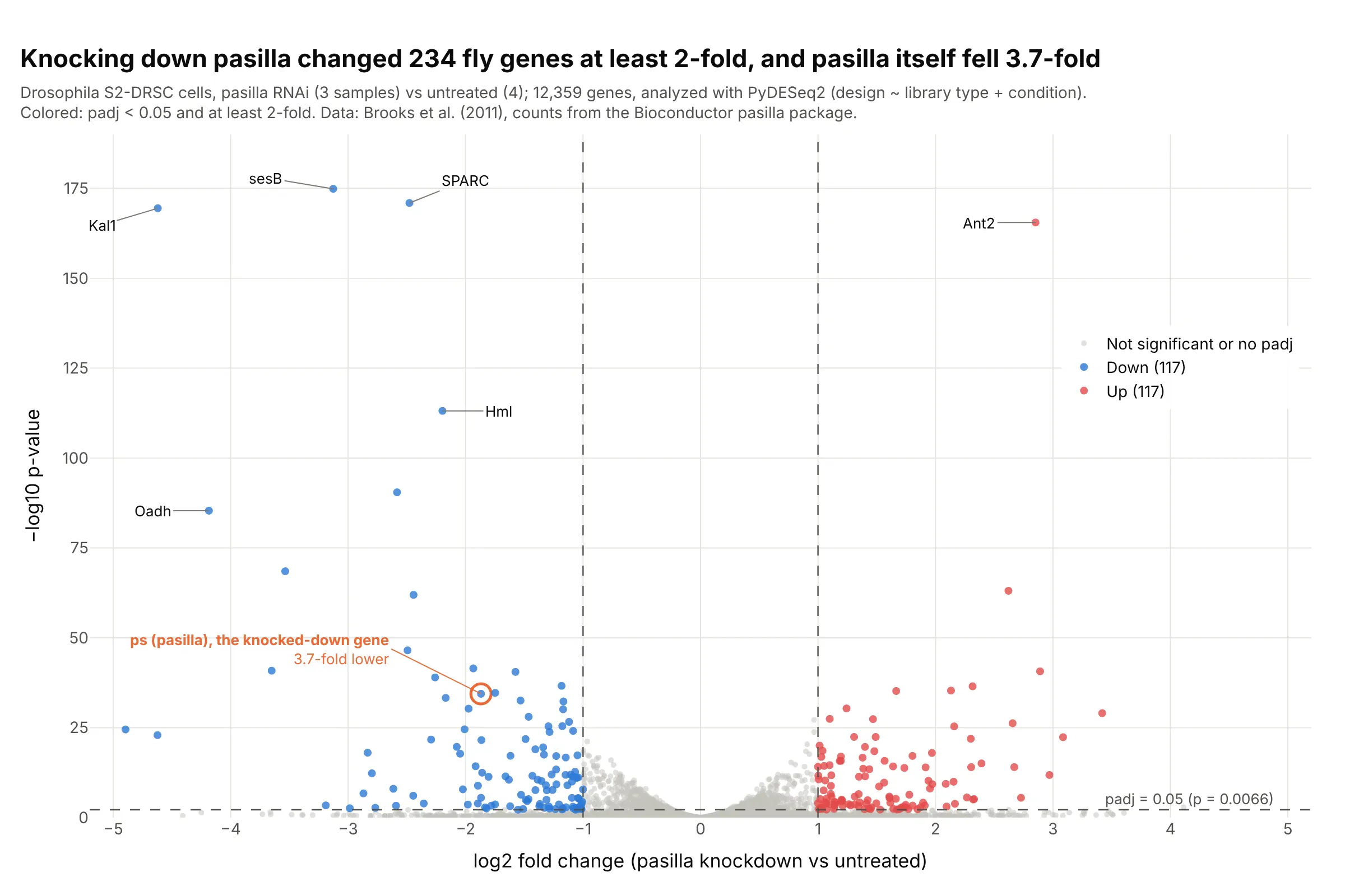
Knocking down the splicing factor pasilla changed 234 genes at least 2-fold, and pasilla itself fell 3.7-fold, which confirms the knockdown worked. This is the dataset the DESeq2 tutorials use, analyzed here with PyDESeq2 in Python. Data: Brooks et al. (2011), counts from the Bioconductor pasilla package.

Tip: circle the gene you perturbed in its own color; if it isn't on the left, check the experiment before the biology.

2. Adverse events in the SELECT semaglutide trial

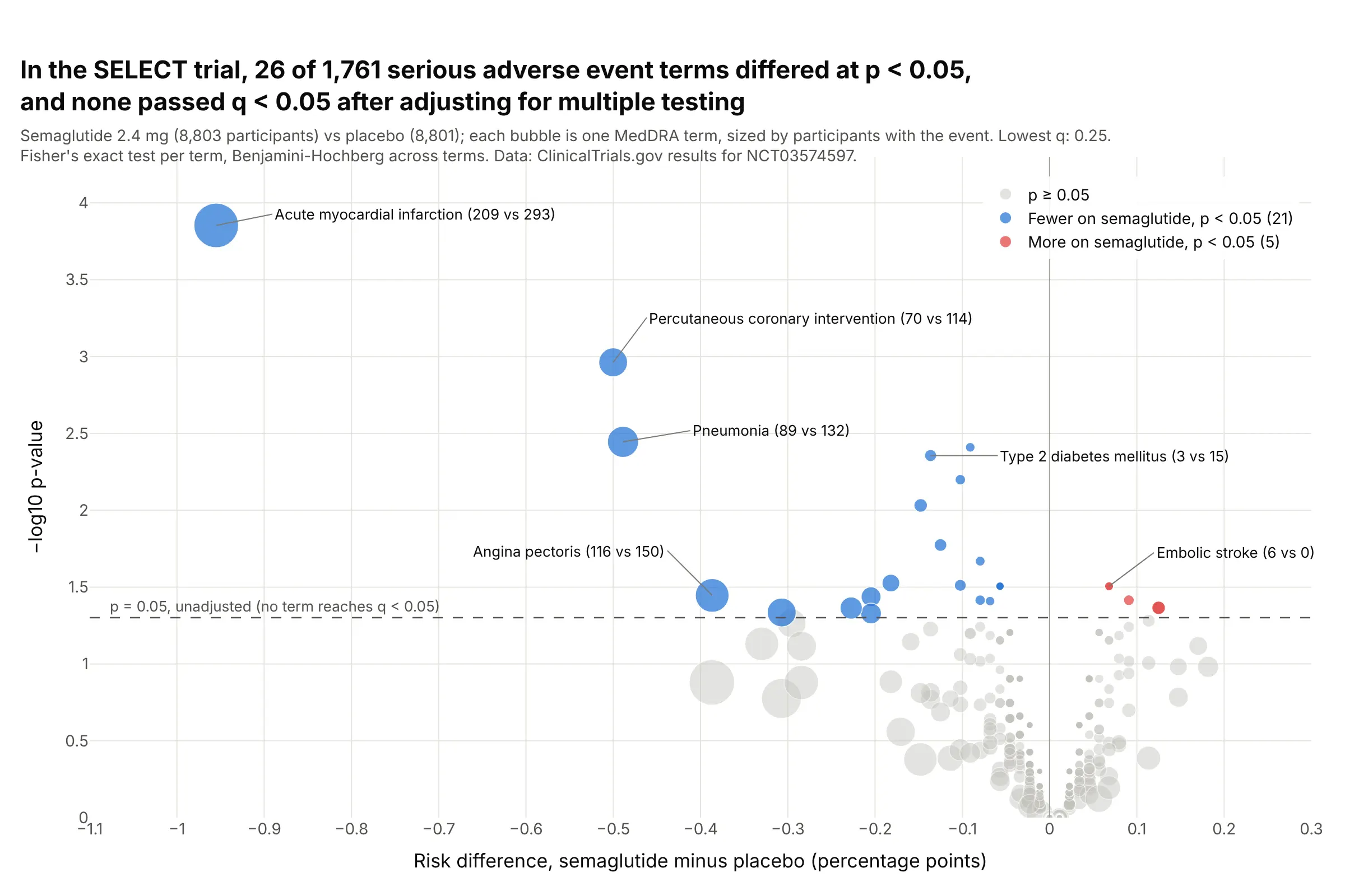
Of 1,761 serious adverse event terms in the 17,604-patient SELECT trial, 26 differed between semaglutide and placebo at p < 0.05, while a 5% false-positive rate alone would allow 88, and none passed q < 0.05. The lowest, acute myocardial infarction (209 vs 293), has q = 0.25. Data: ClinicalTrials.gov results for NCT03574597; method from Zink et al. (2013).

Tip: size each bubble by the number of participants with the event, so a term with 6 cases doesn't look as important as one with 500.

3. Semaglutide's safety signals in FAERS

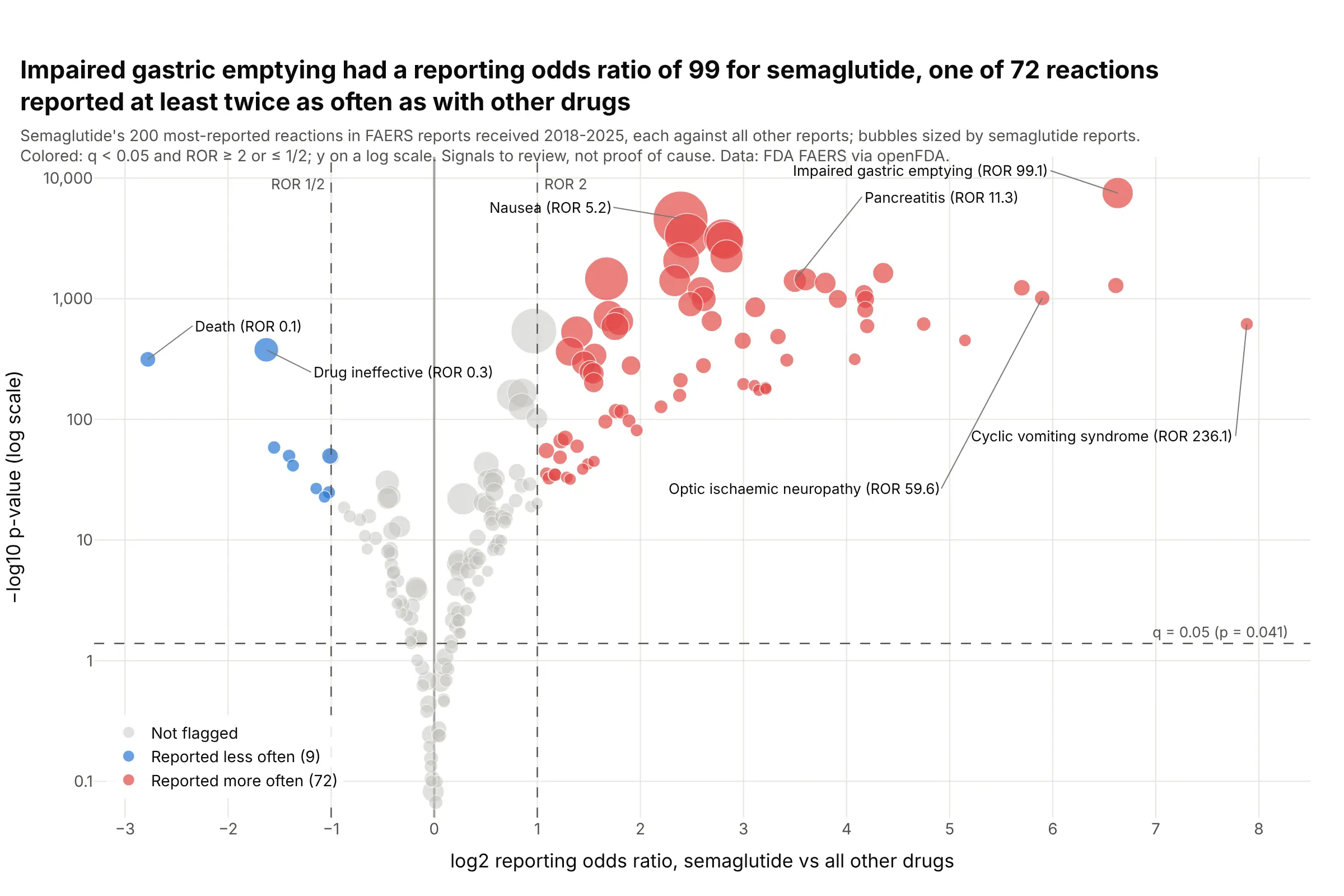
Impaired gastric emptying was reported with semaglutide at 99 times the odds of other drugs in 11.4 million FDA adverse event reports, one of 72 reactions past both thresholds. With this many reports nearly every p-value is tiny, so the fold change threshold does most of the work. Data: FDA Adverse Event Reporting System via openFDA, reports received 2018 to 2025.

Tip: when −log10 p runs into the thousands, use a log y axis.

4. B-cell marker genes in single-cell RNA-seq

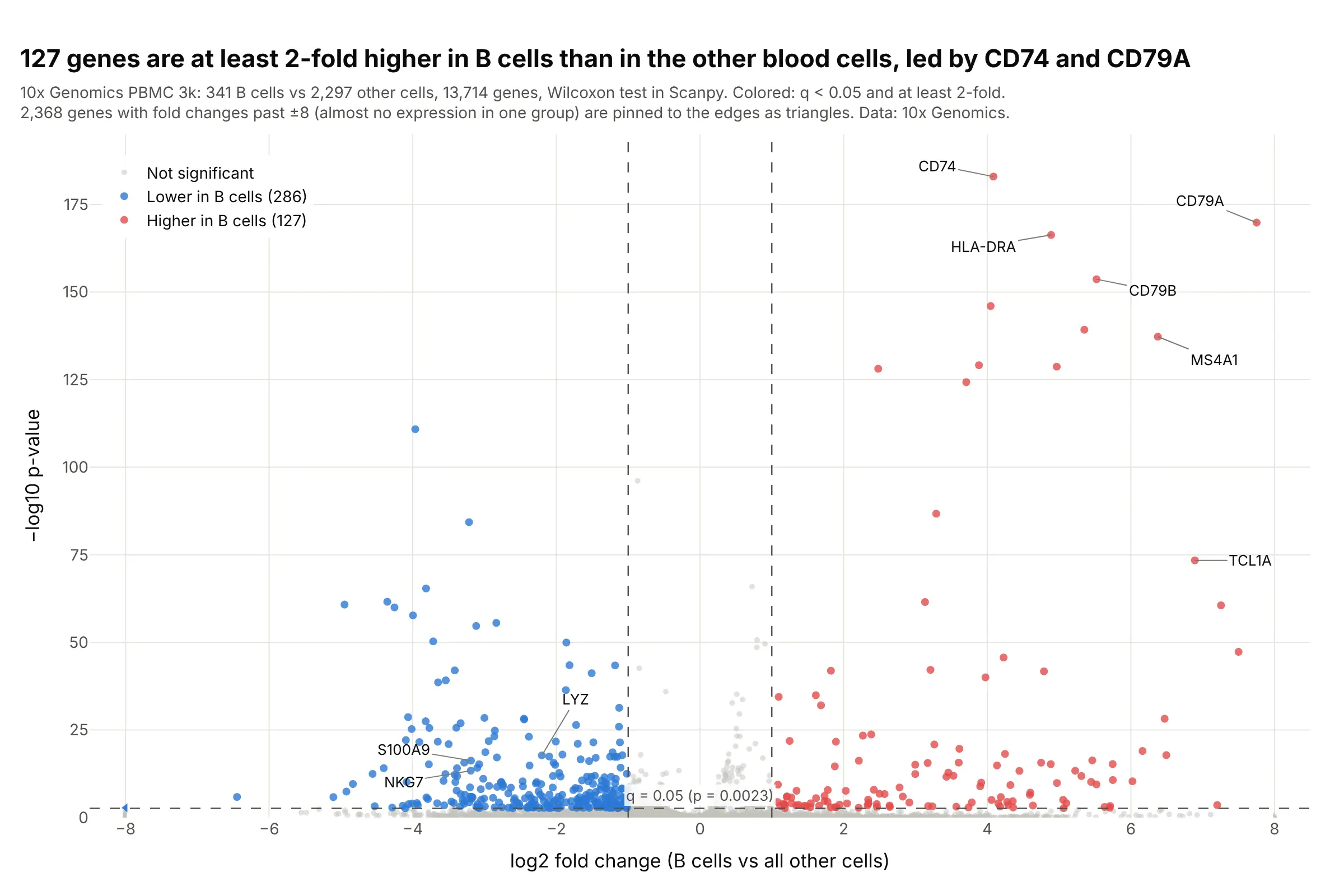
127 genes are at least 2-fold higher in the 341 B cells of 10x Genomics' PBMC 3k dataset than in the other 2,297 cells, led by CD74 and the B-cell receptor gene CD79A. With thousands of cells, p-values reach 10⁻¹⁸³. Data: 10x Genomics PBMC 3k, analyzed with Scanpy.

Tip: single-cell fold changes run to ±27 for genes almost absent in one group, so pin them to the axis edge as triangles instead of stretching the axis.

5. Proteomics over time as small multiples

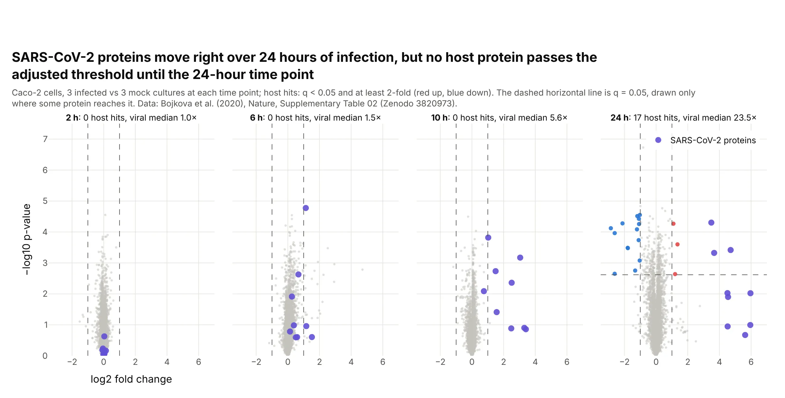
The median viral protein went from 1.0 times its background level at 2 hours to 23.5 times at 24 hours, and no host protein passed q < 0.05 until the 24-hour time point, when 17 changed at least 2-fold. Data: Bojkova et al. (2020), Supplementary Table 02.

Tip: give every panel the same axis ranges, or the cloud will look the same size at every time point.

6. Golub's leukemia microarrays, the classic two-group comparison

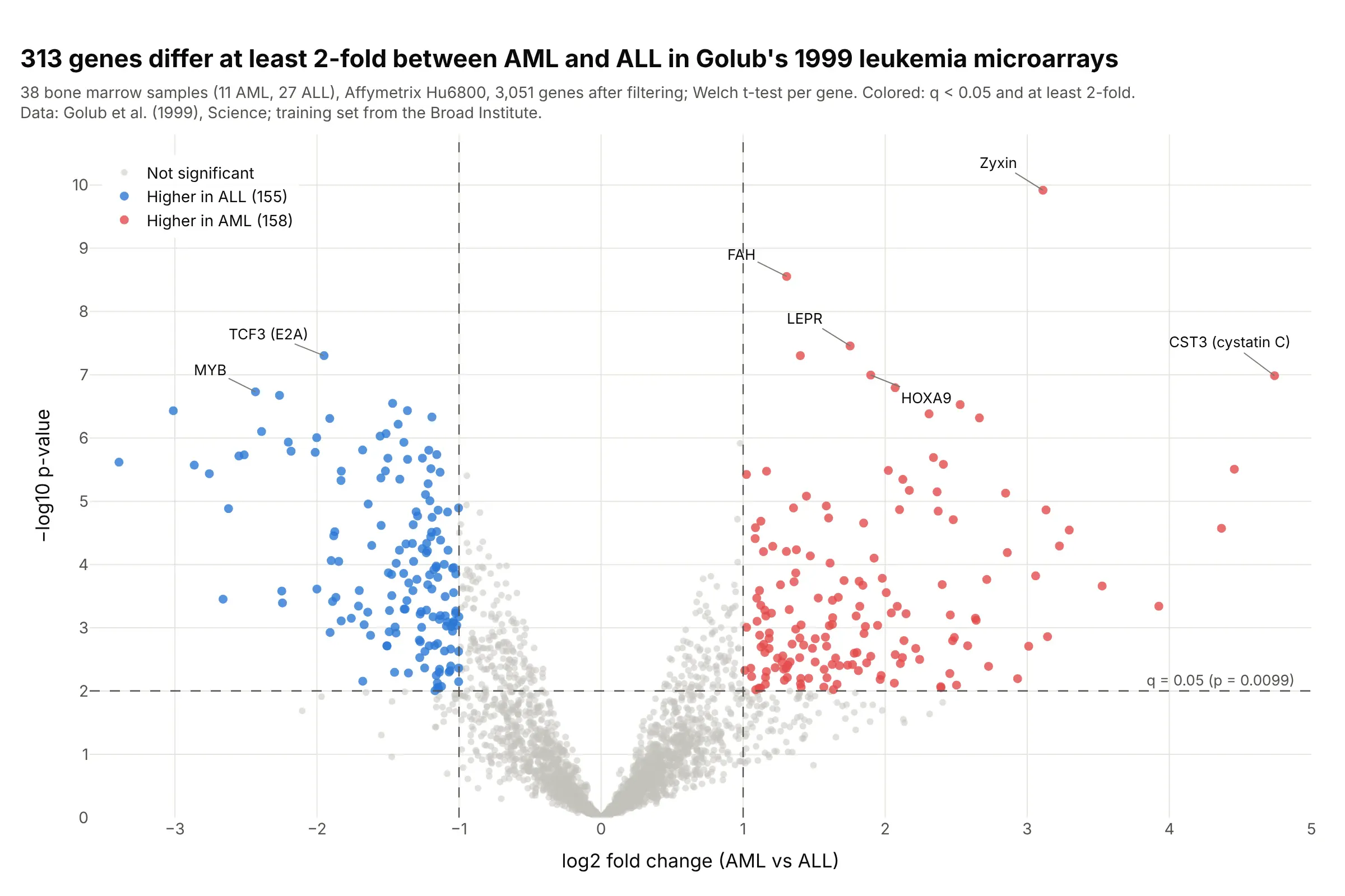
313 genes differ at least 2-fold between acute myeloid and acute lymphoblastic leukemia in Golub's 1999 training set of 38 microarrays, with zyxin the most significant. This is the kind of t-test and fold change comparison the first volcano plots summarized. Data: Golub et al. (1999), training set from the Broad Institute.

Tip: use the same colors, thresholds and axis titles across experiments, so old and new results can be compared at a glance.