
Chris Parmer
November 18, 2026
Type Curves - A Complete Guide
TL;DR
- A type curve shows how a typical new oil or gas well will produce. It lines up many similar wells by months since first production, divides each by its lateral length (the horizontal part of the well), and draws the P10, P50 and P90 of their rates (the high, middle and low cases, where P90 is exceeded by 90% of wells) as a band with a line for the median.
- Type curves are also known as type wells and type well profiles, and are similar to decline curves, which fit an equation to one well, and to fan charts, which show a range around a central forecast. A type curve describes wells that have not been drilled yet, so it feeds well planning, drilling budgets and reserves estimates.
- The details decide whether a type curve can be trusted: use wells that are alike, count only months in which a well produced, say how many wells stand behind each month, and never add up P90 values across wells, because the P90 of a program is far higher than the sum of its parts.
- You can make a type curve with Plotly from three go.Scatter traces, a P10 line, a P90 line filled to it and a P50 line, on a log rate axis. A short helper function is below, and the data in this guide is real: 5,778 Bakken wells from North Dakota.
What is a type curve?
This is a type curve:
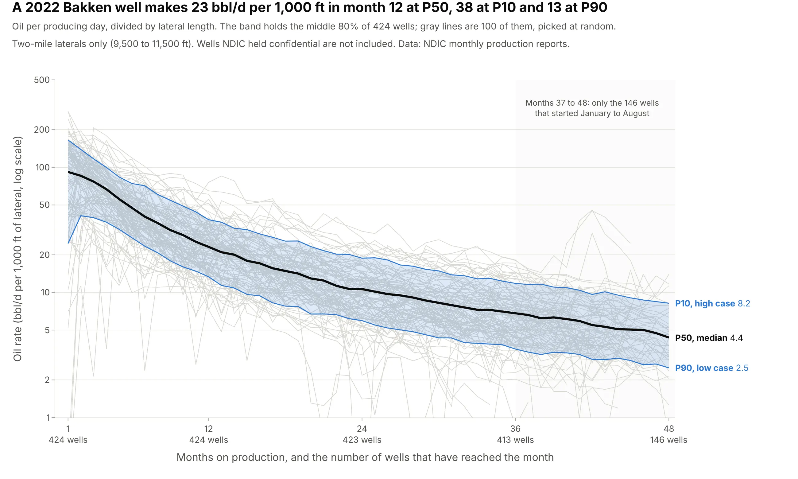
Data: North Dakota Industrial Commission (NDIC), monthly production reports and horizontal wellbore survey lines.
How do you read a type curve? In the example above, notice these things:
- Every thin gray line is one well, plotted by months on production, so each well starts at month 1 no matter when it was drilled. The vertical axis is oil per producing day, divided by the lateral length in thousands of feet, on a log scale where equal steps are equal percentage changes.
- The black P50 line is the median well: half of the wells are above it and half below. It falls from 91.8 barrels a day (bbl/d) per 1,000 ft in month 1 to 23.1 in month 12 and 6.8 in month 36, a drop of 75% in the first year.
- The blue band is the middle 80% of wells. In month 12, 1 well in 10 beats the P10 value of 38.1 and 9 wells in 10 beat the P90 value of 13.3, so the high case is 2.9 times the low case.
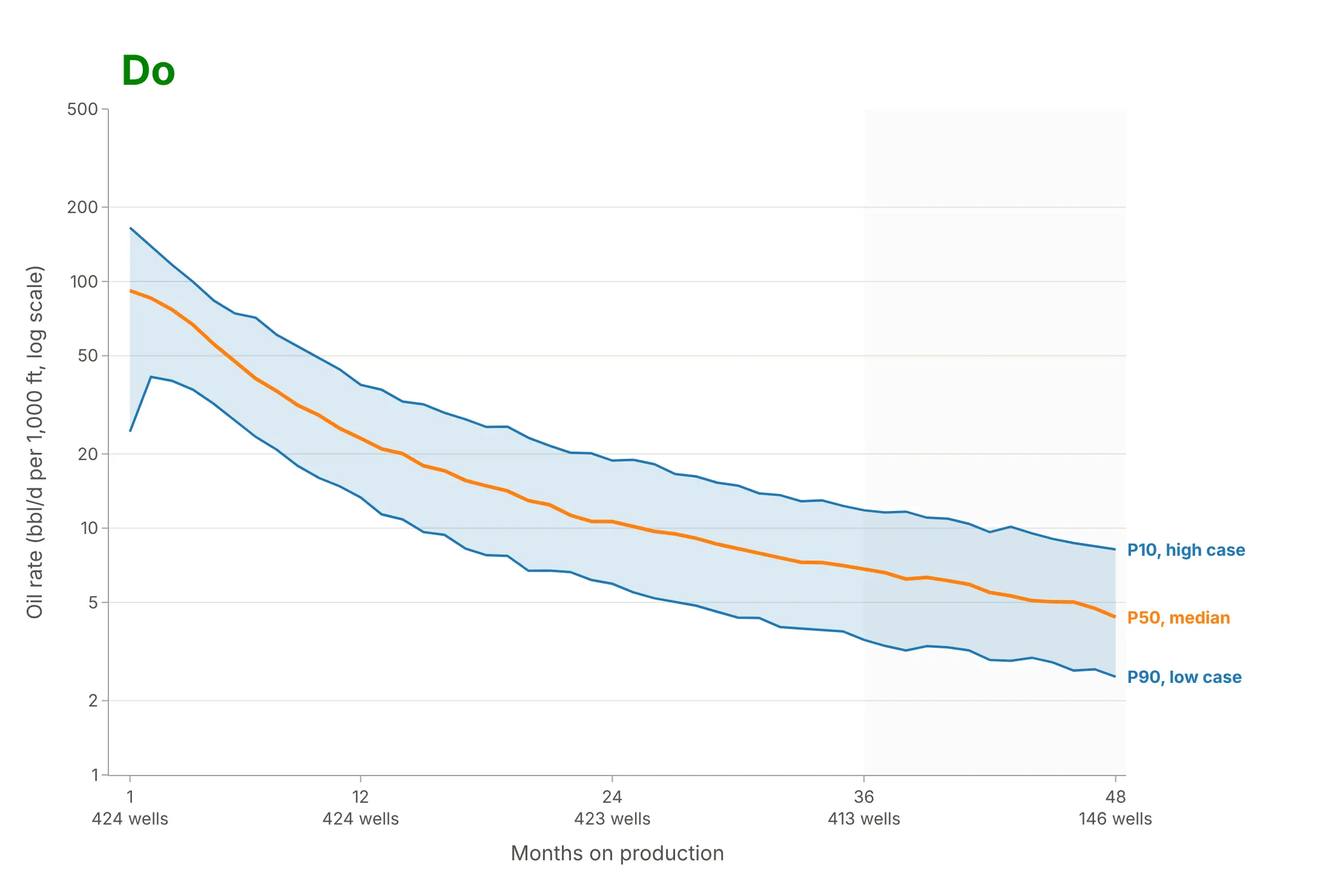
- The axis counts the wells behind each month: 424 wells at month 1, 413 at month 36 and only 146 at month 48, because most 2022 wells have not been producing for 48 months yet. The shaded area is where the curve rests on fewer wells.
It's often used for charts like these:
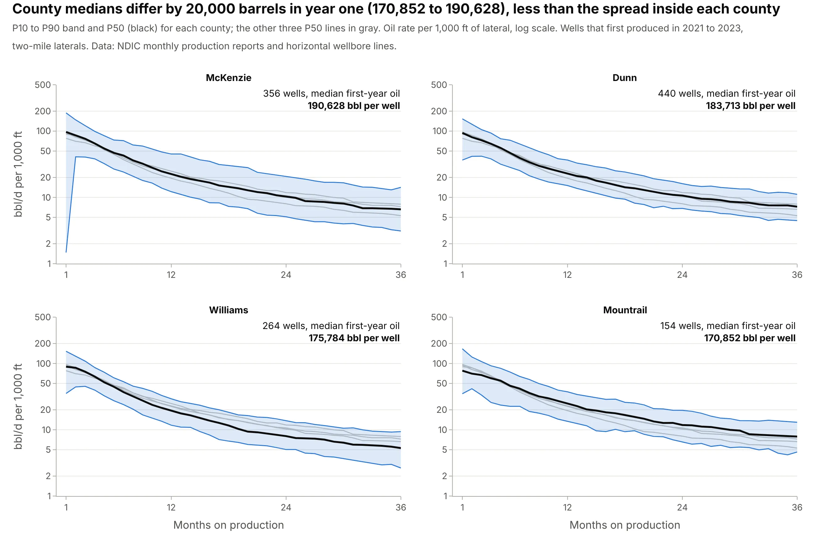
Choosing where to drill. Planners cut one type curve per area, and for wells that started in 2021 to 2023 the median first-year oil of four Bakken counties runs from 170,852 barrels per well in Mountrail County to 190,628 in McKenzie County, a smaller gap than the spread among the wells inside each county. Data: NDIC monthly production reports and horizontal wellbore survey lines.
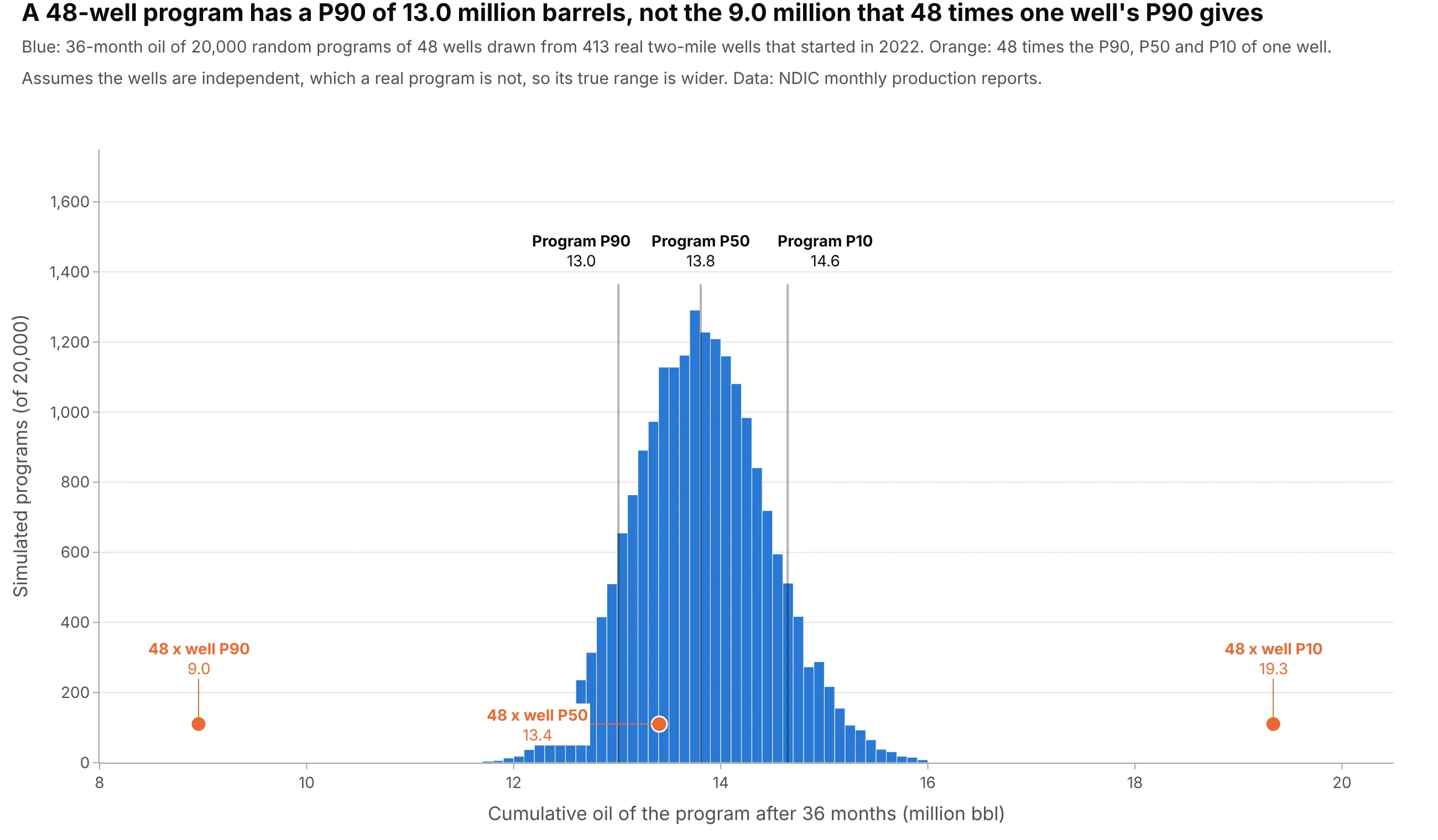
Forecasting a drilling program and booking reserves. A type curve multiplied by the number of wells gives a program forecast, but only the P50 and the mean multiply cleanly: 48 times a single well's P90 is 9.0 million barrels over 36 months, while the P90 of random 48-well programs from the same wells is 13.0 million. Data: NDIC monthly production reports and horizontal wellbore survey lines.
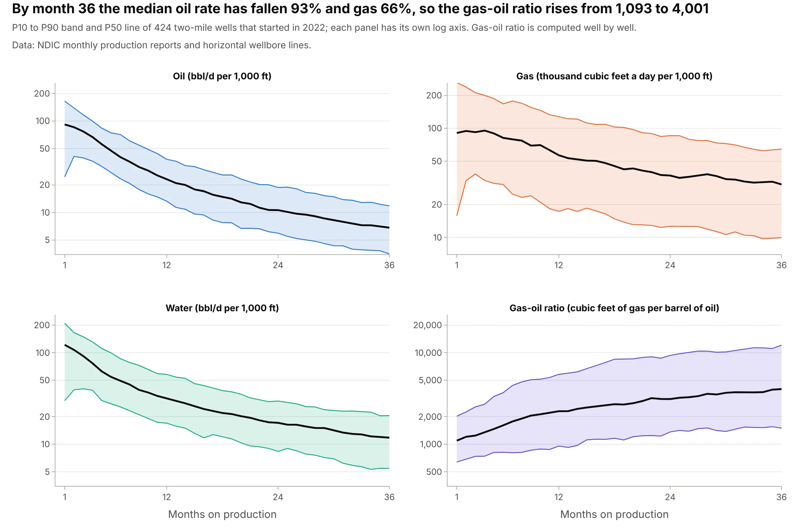
Sizing gas lines and water disposal. Each product has its own type curve, and in the same 2022 wells the median oil rate falls 93% by month 36 while gas falls 66%, so the gas-oil ratio rises from 1,093 to 4,001 cubic feet per barrel. Data: NDIC monthly production reports and horizontal wellbore survey lines.
Reservoir engineers (who estimate how much oil and gas a field will produce), asset teams, lenders and investors use type curves to decide how many wells to drill, where to put the rigs, how much to pay for an acreage position and how much oil and gas to report as reserves. The wells in a type curve are called analogs, because they stand in for a well that does not exist yet.
A short history
Engineers have projected production from analogs for more than a century. In 1918 J.O. Lewis and Carl Beal of the US Bureau of Mines described "appraisal curves" with average, maximum and minimum curves for properties in Oklahoma, an early version of a P50 line with a high and a low case (Lewis and Beal 1918). In 1945 J.J. Arps published the exponential, hyperbolic and harmonic equations that still describe a single well's decline (Arps 1945). The probability labels come from reserves reporting: the Petroleum Resources Management System (PRMS), the reserves classification maintained by the Society of Petroleum Engineers (SPE) and partner societies, asks for a low, best and high estimate with probabilities of exceeding them of at least 90%, 50% and 10% (PRMS 2018, section 2.2.1.2). For shale plays, where thousands of similar wells are drilled, the Society of Petroleum Evaluation Engineers (SPEE) published A Practical Guide to Type Well Profiles as its Monograph 5 in December 2024, which describes percentile-based methods (Viswanathan and Ryan 2025).
Type curve or decline curve?
The two names are often used for the same page of a report, so it helps to separate them. A decline curve is an equation fitted to the production history of one well or one field, and its job is to extrapolate that history. A type curve starts from many wells and describes what a well like them does, including how much wells differ, and its job is to forecast wells before they are drilled. The two meet at the end: once you have a P50 type curve, you can fit an Arps decline to it and extend it to an estimated ultimate recovery (EUR), the total oil a well will produce in its life.
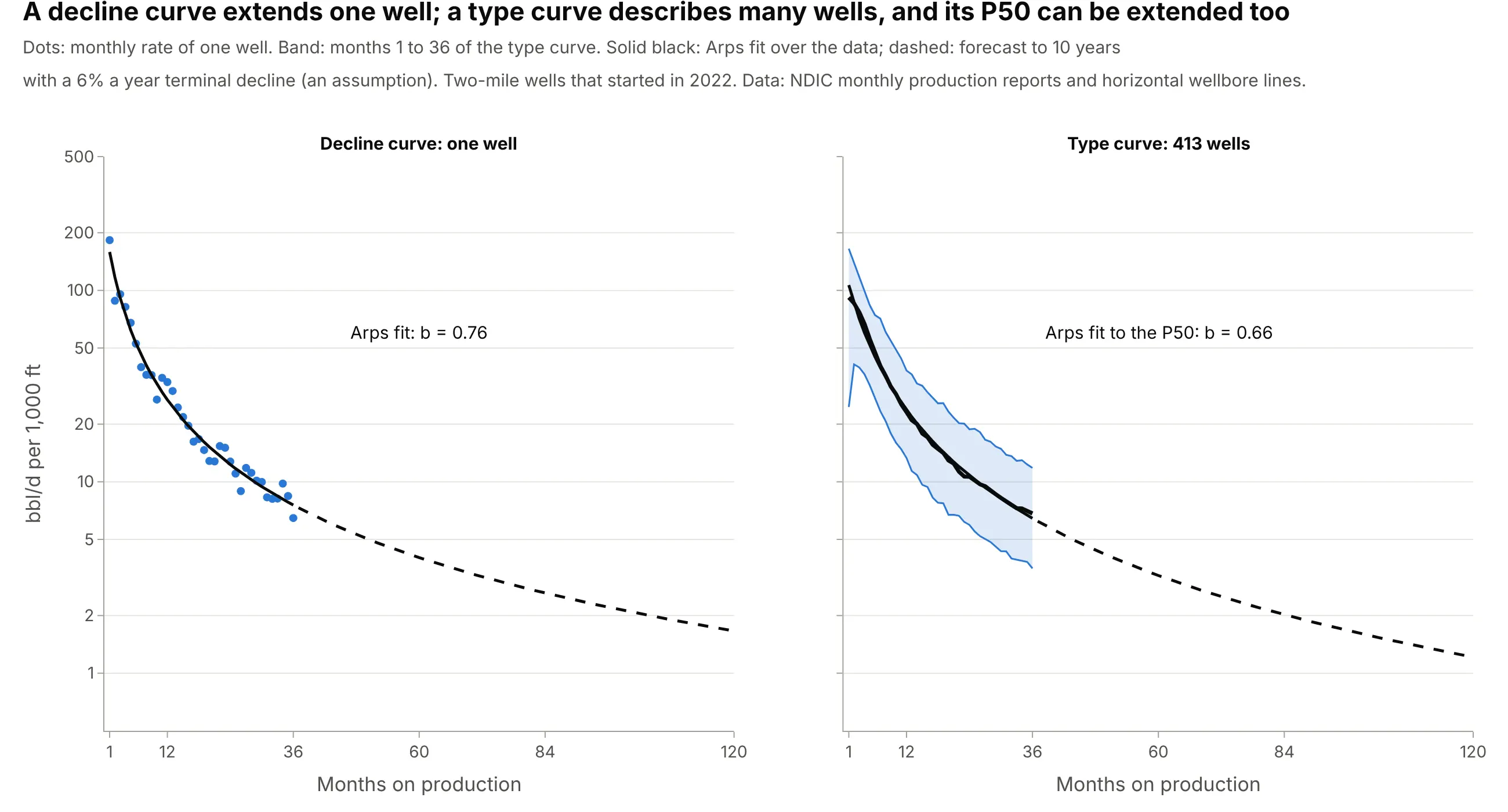
Data: NDIC monthly production reports and horizontal wellbore survey lines; the forecasts assume a terminal decline of 6% a year.
There is a second, older meaning. In 1980 M.J. Fetkovich published "Decline Curve Analysis Using Type Curves", in which a type curve is a standard dimensionless curve that a well's data are matched against (Fetkovich 1980), a way of tying decline equations to reservoir flow. This guide is about the other kind, the P10, P50 and P90 curves built from analog wells.
How a type curve is built
A type curve looks like one smooth statistic, but it hides a series of choices. Each one changes the answer, so it helps to know what to ask the person who built the curve.
1. Pick wells that are alike
The curve is only as good as the claim that these wells are analogs for the next one. The PRMS says analogs should be comparable "in regard to reservoir description, fluid properties, and most likely recovery mechanism(s)" (PRMS 2018, section 4.1.1.1). In practice engineers choose the same formation, area, vintage (the year of first production), completion design and lateral length, and each extra filter leaves fewer wells. For the examples here the formation is the Bakken, the vintage is 2022 and the lateral is the two-mile class, 9,500 to 11,500 ft, which holds 424 of the 509 wells that started that year. The one-mile wells, 4,000 to 6,500 ft, number only 15 in 2022, so they would get a curve of their own with more years of data.
2. Align every well on its first month of production
Wells start at different dates, and a decline that began in March does not line up with one that began in October. A type curve resets each well's clock to month 1 at first production:
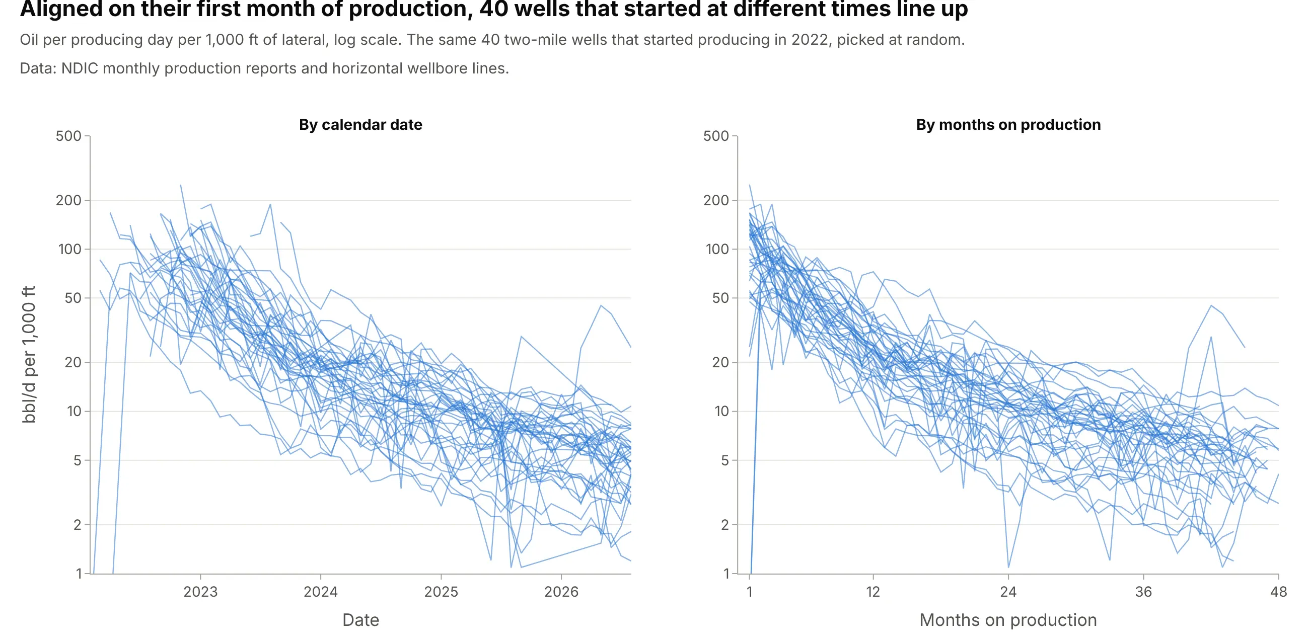
Data: NDIC monthly production reports and horizontal wellbore survey lines.
Months on production count only months in which a well produced, here at least 15 producing days with oil above zero, and the rate is the month's oil divided by its producing days. That way a well that was shut in for a few weeks, which happens for reasons like nearby drilling, doesn't pull the curve down.
3. Divide by lateral length
A longer lateral touches more rock and makes more oil, so type curves are often normalized to a rate per 1,000 ft of lateral, which lets a planner scale the curve to a well of 8,000 or 12,000 ft. This only works within a narrow range of lengths. In the Bakken most laterals are about two miles long: the middle half of 2022 wells run from 10,335 to 10,757 ft, so the division changes little there. It matters more across classes, and example 6 below shows that one-mile wells make 67% more oil per foot than two-mile wells, so normalizing does not turn all wells into equals.
The lateral lengths come from NDIC's horizontal wellbore survey lines. Six of the 509 wells from 2022 have a line shorter than 1,000 ft (the shortest is 211 ft, for a well that produced 271,000 barrels), which cannot be a Bakken lateral, so the survey record is incomplete for them. Wells outside the 9,500 to 11,500 ft class are left out of the main curve.
4. Take percentiles month by month, and read them the oil and gas way
At each month on production, take the rates of all wells and find their percentiles. Statisticians call the value that 90% of wells fall below the 90th percentile. Oil and gas reporting labels values by the chance of beating them: P90 is a low estimate that the actual outcome should equal or exceed with at least 90% probability, and P10 is a high estimate with at least a 10% probability of being equaled or exceeded (PRMS 2018, section 2.2.1.2). So the P10 line is the 90th percentile of the wells and the P90 line is their 10th percentile, which looks backward to anyone trained in statistics:
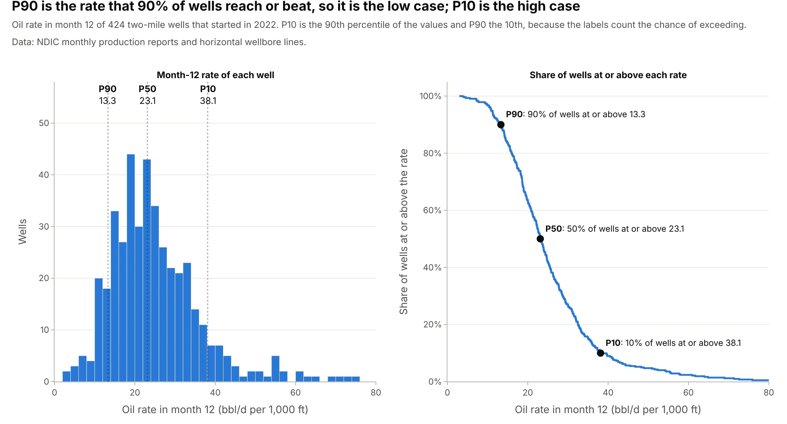
Data: NDIC monthly production reports and horizontal wellbore survey lines.
Reading the right panel from the side explains the labels. At a rate of 13.3 bbl/d per 1,000 ft, 90% of wells are at or above it (P90). At 38.1, only 10% are (P10). If your chart doesn't say which convention it uses, label the lines "P10, high case" and "P90, low case" as the main example does. The same exceedance logic appears in the ECDF plot guide, where the curve is read from the side.
5. Count the wells behind each month, and be honest about survivorship
The wells that have a value at month 48 are not the wells that have one at month 1. Wells fall out of a type curve from the right for two reasons: they are too young to have reached the month, or they have stopped producing. For the 2022 wells, the first reason dominates:
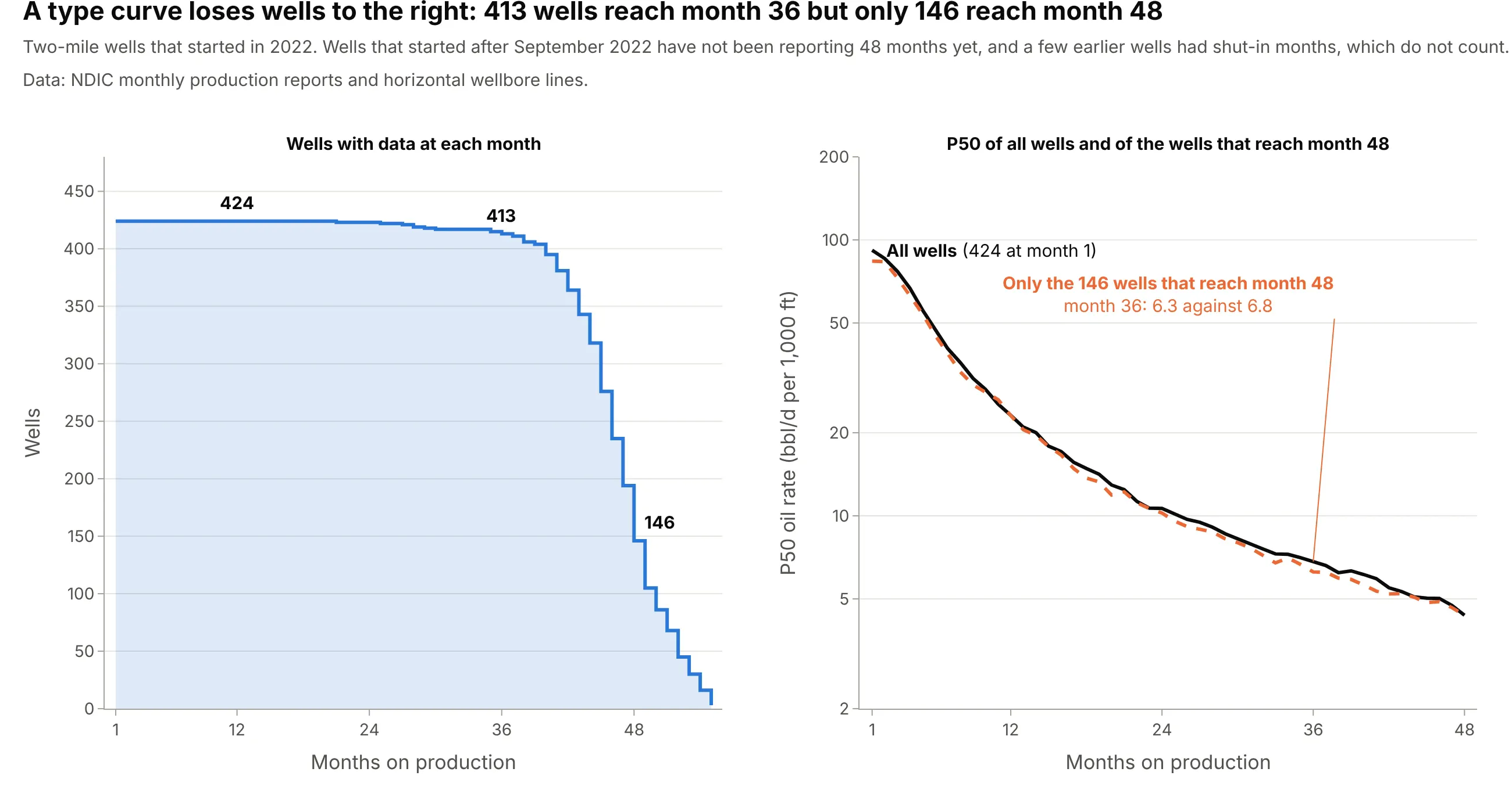
Data: NDIC monthly production reports and horizontal wellbore survey lines.
The P50 at month 48 comes from 146 wells, the ones with 48 producing months by August 2026, and that group's P50 at month 36 is 6.3 bbl/d per 1,000 ft against 6.8 for all wells, so late months lean on a slightly different set of wells. Wells that really stop producing are a smaller effect in this data. Of 680 two-mile wells from 2015 and 2016, 667 reached month 72, and the 13 that did not had a median rate of 9.3 bbl/d per 1,000 ft in month 12 against 16.0 for the 667 that did. The weak wells do drop out first, but they are 2% of the wells here. The NDIC data also leaves out wells that it held confidential: of 9,729 new Bakken wells since June 2015, 3,951 (41%) were confidential at some point and are not in any chart in this guide. We can't tell whether their performance differs from the 5,778 that remain, so treat the curves as a description of the wells that reported openly.
6. Remember that the curve is not a well
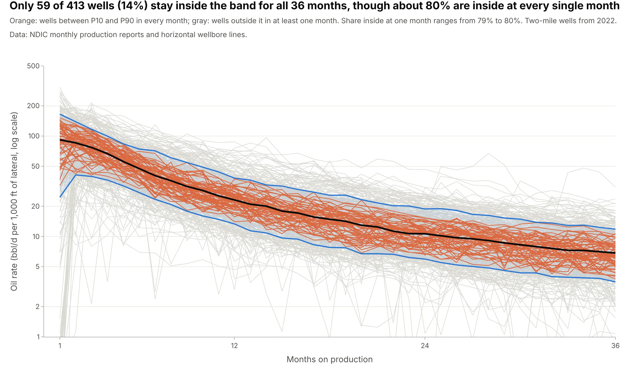
The P50 line is made of the median at each month, and the median at month 3 can come from a different well than the median at month 30. No real well has to follow it. Of 413 wells with 36 months of data, about 80% are inside the P10 to P90 band at any single month, but only 59 of them (14%) stay inside for all 36 months:
Data: NDIC monthly production reports and horizontal wellbore survey lines.
Wells that are high in the first year can be low in the third. Across the 413 wells, the rank of a well in month 12 and its rank in month 36 have a Spearman correlation of 0.57, so early rank predicts later rank only partly. When a model needs one real well, engineers pick a type well, the real well that resembles the curve (example 4 below).
7. Extend it to reserves, with care
Reserves are the volumes a company can report as recoverable. For a US-listed company, the Securities and Exchange Commission (SEC) defines proved reserves with "reasonable certainty", which for probabilistic methods means "at least a 90% probability that the quantities actually recovered will equal or exceed the estimate" (17 CFR 210.4-10), so a P90 case is where proved reserves start. The PRMS ties its low, best and high estimates (P90, P50 and P10) to the categories 1P (proved), 2P (proved plus probable) and 3P (proved plus probable plus possible) in the same way, as one of its criteria (PRMS 2018, section 2.2.2.9).
The catch is aggregation. The PRMS says that in statistical aggregation "the P90 (high degree of certainty) quantities from the aggregate are always greater than the arithmetic sum of the reservoir level P90 quantities" and calls this the portfolio effect (PRMS 2018, section 4.2.5.2). The program example above shows it with real wells: 48 times one well's P90 is 9.0 million barrels, and the P90 of 20,000 random 48-well programs is 13.0 million, 45% higher. The simulation draws wells independently, so it is the best case, since a real program shares an operator, a rig schedule and a set of risks.
Alternatives to a type curve
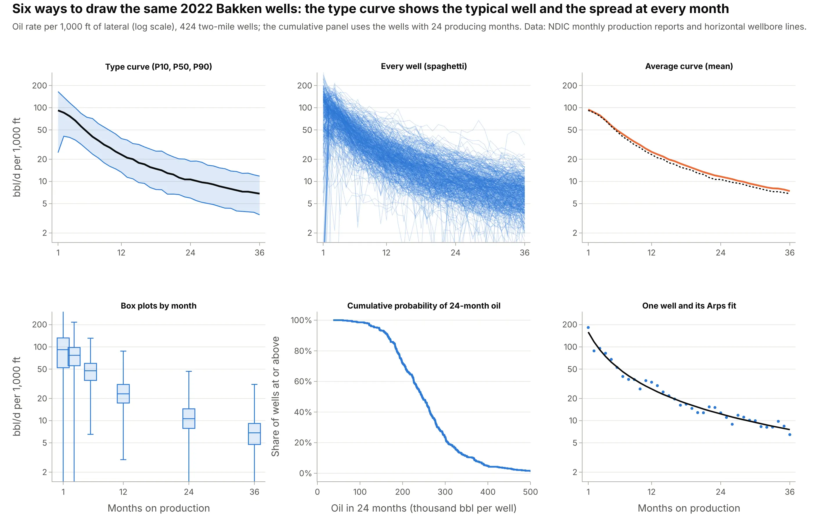
Here's the same 2022 Bakken data drawn six ways. Some are better for the question, some worse, some just different:
Data: NDIC monthly production reports and horizontal wellbore survey lines.
- Type curve with P10, P50 and P90 (better for planning). It shows the typical well and the spread in one picture, and it is the form that feeds forecasts and reserves.
- Every well as a line, a spaghetti plot (works too, as a first look). It shows all the data, but the center and the spread have to be read by eye. The main example draws 100 wells under the band for exactly this reason. It is a case for small multiples or line charts when there are few wells.
- Average curve (different). The mean of the wells is higher than the median here, 25.2 against 23.1 bbl/d per 1,000 ft at month 12, because a few strong wells pull it up. The mean is the right number to multiply by a well count, and the P50 is the right number for the typical well, so say which one you drew.
- Box plots by month (works too, for a few months). A box plot at selected months shows quartiles and outliers, but a type curve shows every month and has the shape of the decline.
- Cumulative probability of an outcome (better for risk). An ECDF of 24-month oil shows the chance of reaching a target volume directly, but it has lost the timing.
- A single decline curve (different). One well's decline curve with its Arps fit is the right tool for a producing well, and the wrong one for a well not yet drilled.
How to make a type curve
With AI
ChatGPT, Claude Code, GitHub Copilot, Cursor and other AI tools are excellent at writing Plotly code. Name Plotly in the prompt, and say which wells belong in the curve, how to align and normalize them and which percentiles to draw:
Make a plotly type curve from well_months.csv (columns: api, pmonth, oil_bbl, days, lateral_ft; one row per producing month).- Rate = oil_bbl / days / (lateral_ft / 1000), pivoted to one row per well and one column per month on production (pmonth).- Draw P10 (90th percentile), P90 (10th percentile) and P50 (median) at each month with go.Scatter: P10 and P90 as thin blue lines with fill="tonexty" between them, P50 as a bold black line. Log y axis.- Label the lines "P10, high case", "P50, median" and "P90, low case" at the right end.- Put the number of wells with data under the x tick labels, and shade the months with fewer than half of the wells.- Check: print the P10, P50 and P90 at month 12 and the number of wells at months 1, 12, 24 and 36.
With Plotly Studio
Plotly Studio is a product for creating data visualizations and Dash apps and for analyzing data with AI, available as a desktop app or embedded in Dash apps. Ask for a type curve the same way:
Show a type curve of oil rate per 1,000 ft of lateral by months on production for wells that started in 2022, with a P10 to P90 band, a bold P50 line, a log rate axis, the number of wells under each tick, and a dropdown to pick the county.
Make a type curve in Python or JavaScript
This is the code AI tools write under the hood. Plotly has no dedicated type curve trace, so a type curve is three go.Scatter traces: the P10 line, the P90 line filled up to it with fill="tonexty", and the P50 line. This helper returns a go.Figure, and every example in this guide builds on the same idea:
import numpy as npimport pandas as pdimport plotly.graph_objects as godef type_curve(wells, months=None, p10="#2a78d6"):"""A type curve in Plotly: P10, P50 and P90 of many wells by month on production.`wells` has one row per well and one column per month on production (a rate per 1,000 ft of lateral).P10 is the high case (the 90th percentile of the values), P90 the low case (the 10th percentile)."""cols = wells.columns if months is None else monthsq = wells[cols].quantile([0.9, 0.5, 0.1]) # P10, P50, P90n = wells[cols].notna().sum()fig = go.Figure([go.Scatter(x=cols, y=q.loc[0.9], mode="lines", line=dict(color=p10, width=1.5), name="P10, high case"),go.Scatter(x=cols, y=q.loc[0.1], mode="lines", line=dict(color=p10, width=1.5), name="P90, low case",fill="tonexty", fillcolor="rgba(42,120,214,0.16)"),go.Scatter(x=cols, y=q.loc[0.5], mode="lines", line=dict(color="#0b0b0b", width=3.5), name="P50, median",customdata=n, hovertemplate="Month %{x}<br>P50 %{y:.1f}<br>%{customdata} wells<extra></extra>"),])fig.update_yaxes(type="log", title="Oil rate (bbl/d per 1,000 ft of lateral)")fig.update_xaxes(title="Months on production")fig.update_layout(template="simple_white", showlegend=False)return fig# One row per well-month: api, pmonth (months on production), oil_bbl, days (producing days), lateral_ftdf = pd.read_csv("well_months.csv")df["rate_per_1000ft"] = df.oil_bbl / df.days / (df.lateral_ft / 1000)wells = df.pivot(index="api", columns="pmonth", values="rate_per_1000ft").loc[:, :48]type_curve(wells).show()
For a cumulative type curve, take df.groupby("api").oil_bbl.cumsum() before pivoting. To extend the P50 to an EUR, fit an Arps decline to it with scipy.optimize.curve_fit as in the decline curve guide and add a dashed forecast trace.
In JavaScript, plotly.js draws the same thing with three scatter traces. The arrays below are the P10, P50 and P90 of the first 24 months of the main example:
<div id="chart"></div><script src="https://cdn.plot.ly/plotly-4.1.1.min.js"></script><script>// Oil rate (bbl/d per 1,000 ft of lateral) of 424 Bakken wells that started in 2022, months 1 to 24 (NDIC)const p10 = [165.2, 138.7, 116.9, 99.8, 83.6, 74.2, 71.2, 60.8, 54.6, 49.4, 44.0, 38.1, 36.4, 32.6, 31.8, 29.4, 27.6, 25.7, 25.8, 23.2, 21.6, 20.2, 20.1, 18.8];const p50 = [91.8, 85.6, 76.9, 66.8, 55.7, 47.5, 40.4, 35.9, 31.5, 28.7, 25.4, 23.1, 21.0, 20.0, 17.9, 17.1, 15.6, 14.8, 14.2, 12.9, 12.4, 11.3, 10.7, 10.6];const p90 = [24.6, 41.0, 39.6, 36.4, 31.9, 27.3, 23.4, 20.8, 17.9, 16.0, 14.8, 13.3, 11.4, 10.9, 9.6, 9.4, 8.3, 7.8, 7.7, 6.7, 6.7, 6.6, 6.2, 6.0];const month = p50.map((_, i) => i + 1);Plotly.newPlot("chart", [{x: month, y: p10, mode: "lines", line: {color: "#2a78d6", width: 1.5}, name: "P10, high case"},{x: month, y: p90, mode: "lines", line: {color: "#2a78d6", width: 1.5}, name: "P90, low case",fill: "tonexty", fillcolor: "rgba(42,120,214,0.16)"},{x: month, y: p50, mode: "lines", line: {color: "#0b0b0b", width: 3.5}, name: "P50, median"}], {width: 900, height: 500, template: "simple_white", showlegend: false,xaxis: {title: {text: "Months on production"}},yaxis: {type: "log", title: {text: "Oil rate (bbl/d per 1,000 ft of lateral)"}}});</script>
Share it
Every Plotly chart has a Share chart button (the cloud icon in its toolbar) that uploads it to Plotly Cloud and gives you a link. Only you can see it until you change its visibility.
For a live app, put the chart in a Dash app and publish it with the Plotly Cloud CLI. Coding agents can run these commands for you:
pip install "dash[cloud]"plotly user loginplotly app publish
If your data has to stay in your own cloud or data center, publish to Dash Enterprise instead.
Dos and don'ts
Most of the work in a published type curve is getting the labels and the counts right, because the wells and the arithmetic are shared by good and bad versions. Here are the 2022 Bakken wells both ways.
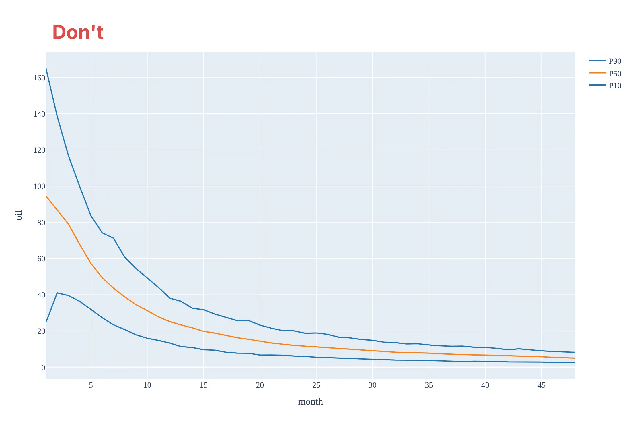
Don't draw the curve on a linear axis, which squashes the tail where most of the production's life is spent, label the high case as P90, draw the mean and call it P50, hide how many wells stand behind each month, or keep the default fonts, a legend of unrelated trace names and raw axis titles:
Do use a log rate axis, label P10 as the high case and P90 as the low case, draw the median as P50, count the wells under the ticks and shade the months that rest on fewer wells:
Checklist
Do
- Choose analog wells that match on formation, area, vintage, completion and lateral length, and say so.
- Align on the first month of production and count producing months only.
- Take percentiles month by month and label P10 as the high case and P90 as the low case.
- Show how many wells stand behind each month, and mark where the count falls.
- Back-test the curve on wells drilled later, and refresh it when the design changes.
Don't
- Add up P90 values across wells to get a program P90.
- Build a curve only from the wells that have survived the longest, or only from the best wells.
- Mix lateral length classes and call it a rate per 1,000 ft.
- Present the P50 line as if it were a real well.
- Extrapolate a hyperbolic decline forever without a terminal decline.
More type curve examples
1. Tracking new wells against the type curve
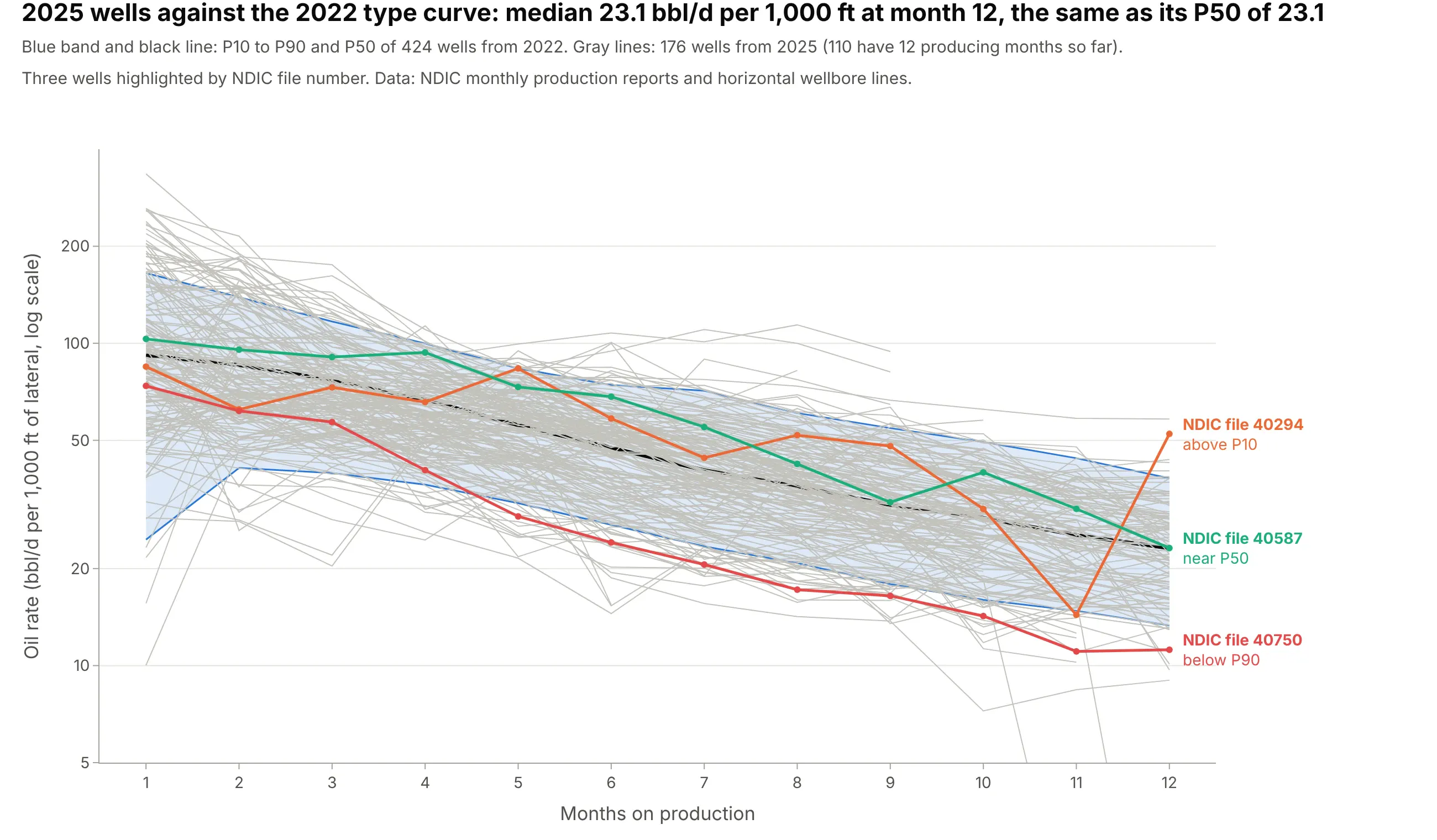
Operations teams plot every new well on the type curve to see whether it is on type. The 176 wells that started in 2025 land across the whole 2022 band, and the 110 that have 12 producing months so far have a median of 23.1 bbl/d per 1,000 ft, the same as the 2022 P50 of 23.1. Data: NDIC monthly production reports and horizontal wellbore survey lines.
Tip: Compare wells at the same month on production and label the few outliers by well name or ID, so an engineer can pull up the well.
Get the data from the North Dakota Industrial Commission's monthly production reports (https://www.dmr.nd.gov/oilgas/mprindex.asp, one Excel file per month, sheet "Oil", columns API_WELLNO, FileNo, ReportDate, Oil, Days, Pool) and its horizontal wellbore lines layer for lateral length. Make a plotly chart of the oil rate per 1,000 ft of lateral of Bakken wells that started in 2025, as thin gray lines by month on production over the P10 to P90 band and P50 of wells that started in 2022, and highlight three wells by file number.
2. Back-testing a type curve
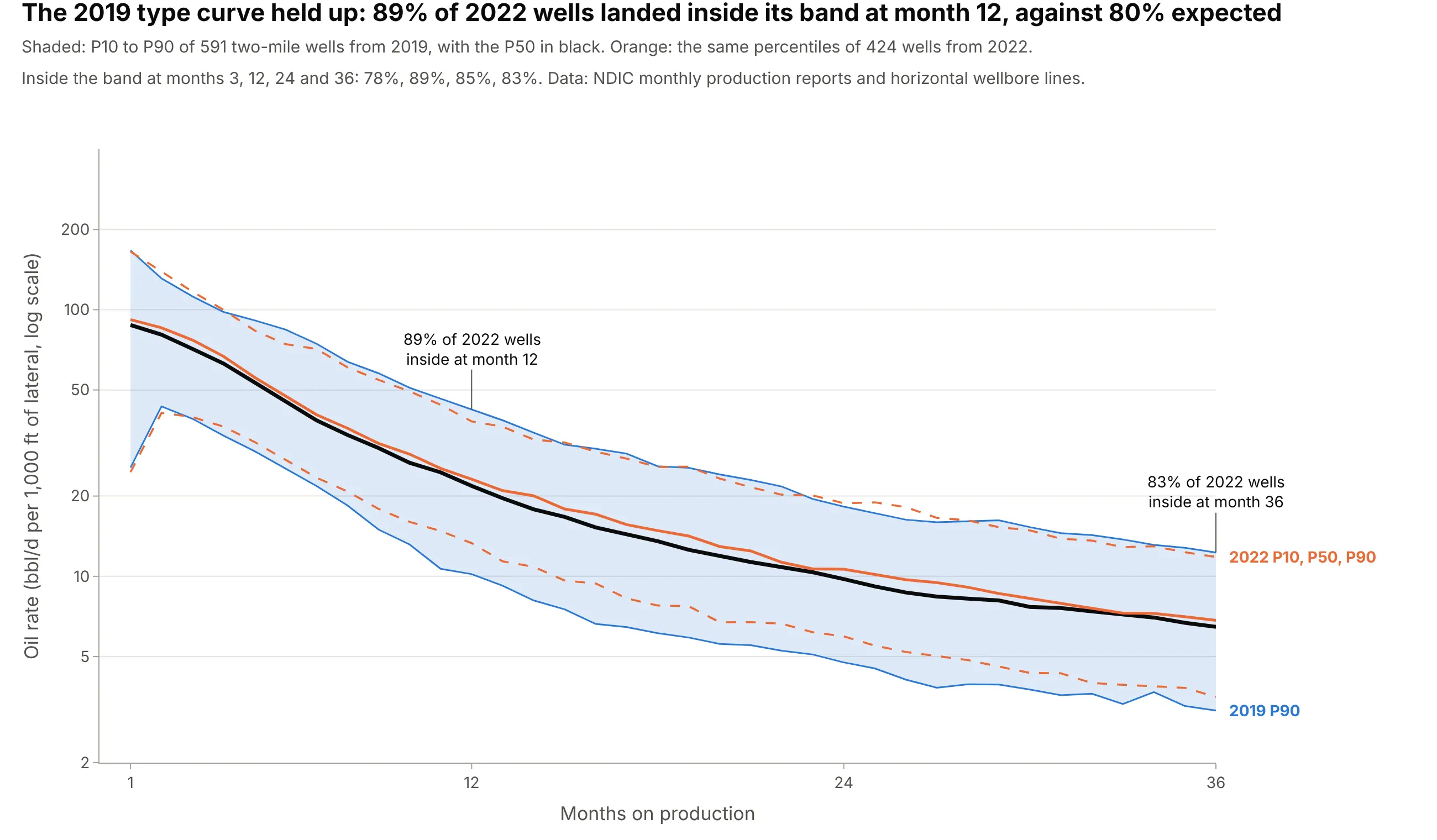
A type curve is a forecast for wells not yet drilled, so you can test it. The 2019 band caught 89% of the 2022 wells at month 12, where a calibrated 80% band would catch 80%, and 83% at month 36, and the 2019 P50 of 21.8 was close to the 2022 P50 of 23.1. The band was a little wider than it needed to be. Data: NDIC monthly production reports and horizontal wellbore survey lines.
Tip: Report the share of later wells inside the band, month by month, next to the curve.
Get the data from the North Dakota Industrial Commission's monthly production reports (https://www.dmr.nd.gov/oilgas/mprindex.asp, sheet "Oil", columns API_WELLNO, ReportDate, Oil, Days, Pool) and its horizontal wellbore lines layer. Make a plotly chart that draws the P10 to P90 band and P50 of Bakken wells that started in 2019 and over it the P10, P50 and P90 of wells that started in 2022, per 1,000 ft of lateral, months 1 to 36. Print the share of 2022 wells inside the 2019 band at months 3, 12, 24 and 36.
3. Type curves go stale
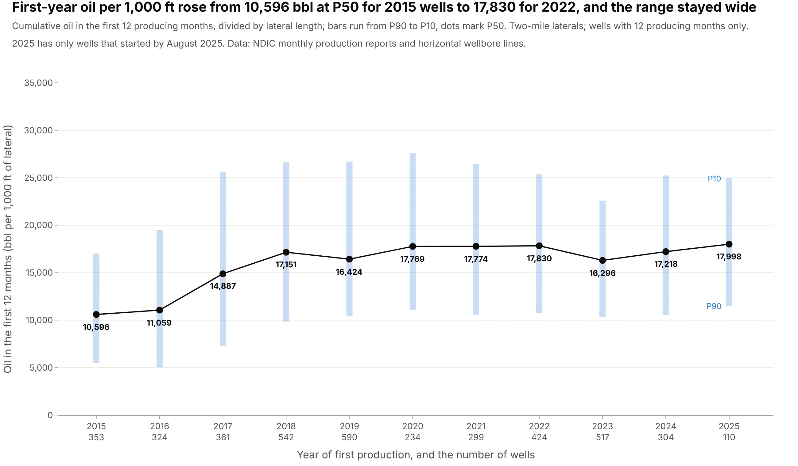
Operators re-cut their type curves because the wells keep changing. The median first-year oil per 1,000 ft of lateral rose from 10,596 bbl for 2015 wells to 17,830 bbl for 2022 wells, while the P10 to P90 range around it stayed wide, from 10,737 to 25,361 bbl in 2022. Data: NDIC monthly production reports and horizontal wellbore survey lines.
Tip: Put the number of wells under each year, since the newest year rests on the fewest wells.
Get the data from the North Dakota Industrial Commission's monthly production reports (https://www.dmr.nd.gov/oilgas/mprindex.asp, sheet "Oil", columns API_WELLNO, ReportDate, Oil, Days, Pool) and its horizontal wellbore lines layer. For Bakken wells with a 9,500 to 11,500 ft lateral and 12 producing months, make a plotly chart of cumulative oil in the first 12 months per 1,000 ft of lateral by year of first production, 2015 to 2025: a bar from P90 to P10 and a dot at P50 for each year, with the well count under each year.
4. A type well, the real well closest to the P50
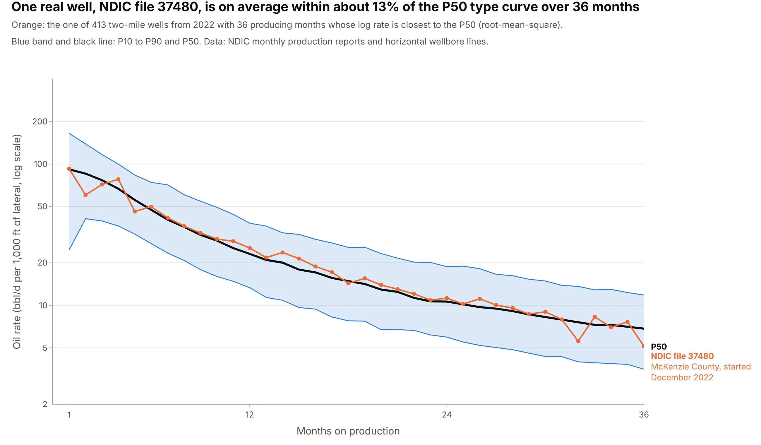
Because the P50 line is not one well, models that need one set of well data pick a type well. The well with the smallest average log distance from the P50 over months 1 to 36 among 413 wells is NDIC file 37480 in McKenzie County, which started in December 2022 and is on average within about 13% of the P50 (root-mean-square, on a log scale). Data: NDIC monthly production reports and horizontal wellbore survey lines.
Tip: Measure the distance on a log scale, so that a miss of 10% counts the same at 80 bbl/d and at 8 bbl/d.
Get the data from the North Dakota Industrial Commission's monthly production reports (https://www.dmr.nd.gov/oilgas/mprindex.asp, sheet "Oil", columns API_WELLNO, FileNo, ReportDate, Oil, Days, County, Pool) and its horizontal wellbore lines layer. For Bakken wells from 2022 with a 9,500 to 11,500 ft lateral and 36 producing months, compute the P50 per 1,000 ft of lateral, find the well with the smallest root-mean-square difference of log rate from the P50, and make a plotly chart of that well over the P10 to P90 band and P50.
5. From a type curve to EUR
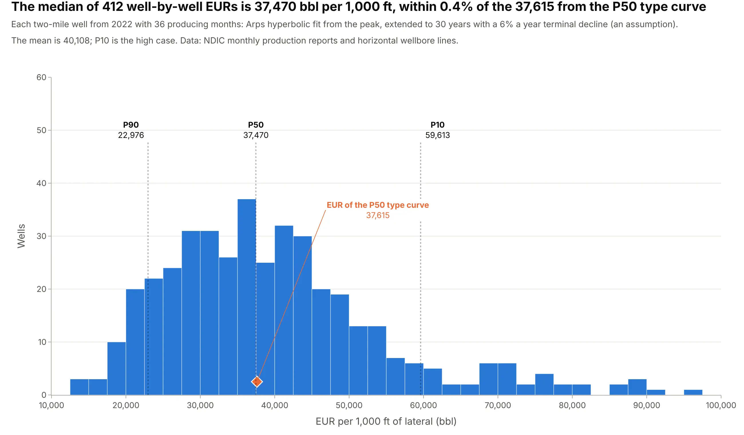
There are two ways to get an EUR from the same wells. Fitting an Arps decline to each of 412 wells gives a median EUR of 37,470 bbl per 1,000 ft, and fitting one to the P50 type curve gives 37,615, within 0.4%. Both extend 36 months of data to 30 years with a 6% a year terminal decline, which is an assumption, and the per-well spread is wide: P10 is 59,613 and P90 is 22,976 bbl per 1,000 ft. Data: NDIC monthly production reports and horizontal wellbore survey lines.
Tip: Say which assumptions end the forecast, because a hyperbolic decline with no terminal decline gives a much larger EUR.
Get the data from the North Dakota Industrial Commission's monthly production reports (https://www.dmr.nd.gov/oilgas/mprindex.asp, sheet "Oil", columns API_WELLNO, ReportDate, Oil, Days, Pool) and its horizontal wellbore lines layer. For Bakken wells from 2022 with a 9,500 to 11,500 ft lateral and 36 producing months, fit an Arps hyperbolic decline to each well's rate per 1,000 ft from its peak, extend it to 30 years with a 6% a year terminal decline, and make a plotly histogram of the EURs with dotted lines at P10, P50 and P90 and a marker for the EUR of the P50 type curve.
6. Does dividing by lateral length work?
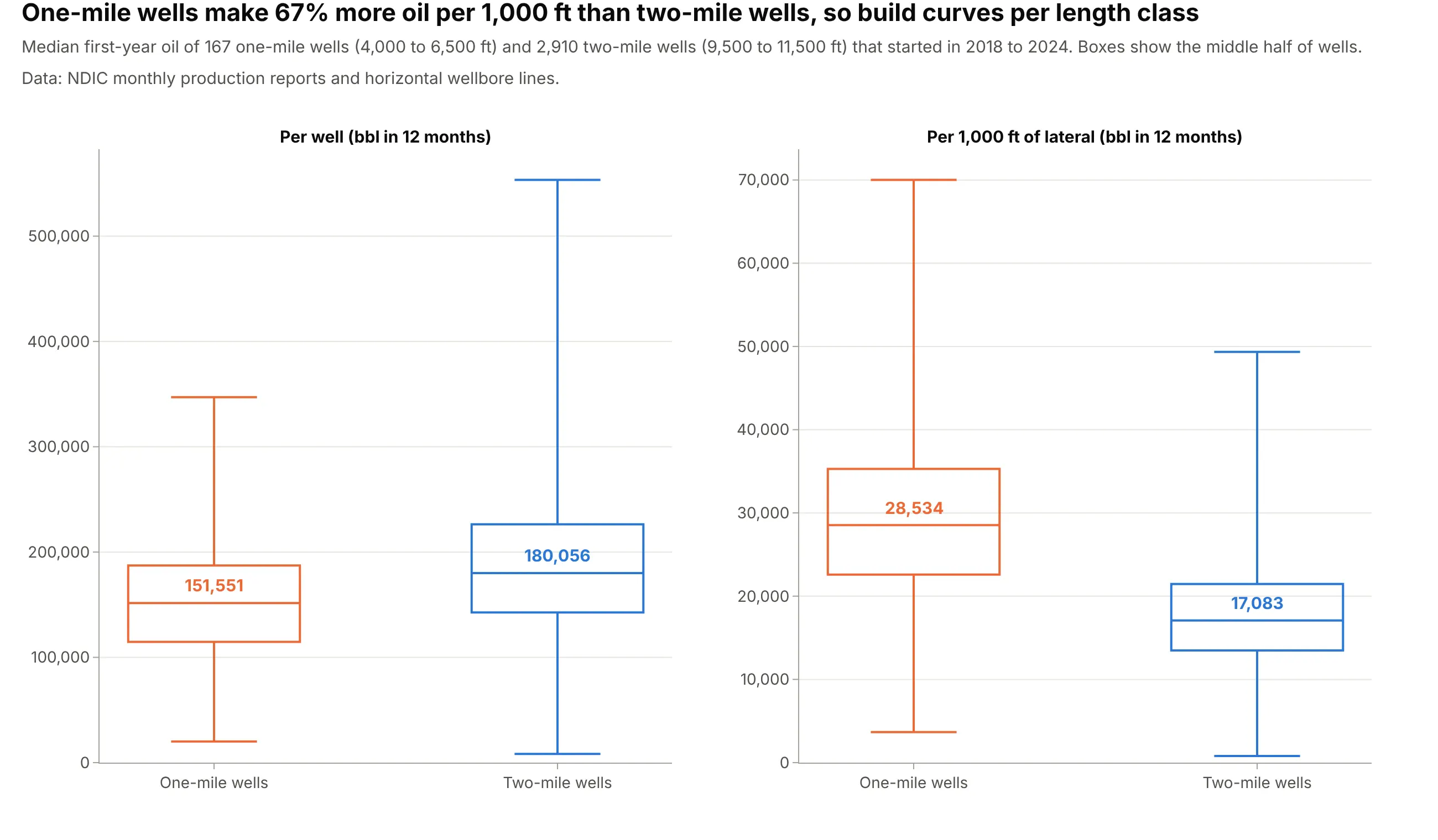
Per-foot normalization assumes oil scales with length, and the data say otherwise. The median first-year oil of 167 one-mile wells that started in 2018 to 2024 is 151,551 bbl, 84% of the 180,057 bbl of 2,910 two-mile wells with half the lateral, so per 1,000 ft the one-mile wells make 67% more. The data don't say why, so build curves per length class. Data: NDIC monthly production reports and horizontal wellbore survey lines.
Tip: Show the raw and the normalized numbers side by side, so readers can see what the division did.
Get the data from the North Dakota Industrial Commission's monthly production reports (https://www.dmr.nd.gov/oilgas/mprindex.asp, sheet "Oil", columns API_WELLNO, ReportDate, Oil, Days, Pool) and its horizontal wellbore lines layer. For Bakken wells that started in 2018 to 2024 with 12 producing months, split them into one-mile (4,000 to 6,500 ft) and two-mile (9,500 to 11,500 ft) laterals and make plotly box plots of cumulative first-year oil per well and per 1,000 ft of lateral, with the medians labeled.
FAQ
Options to customize
- fill="tonexty" on the P90 trace: shades the band down from the P10 trace drawn before it. See Scatter traces in the Plotly reference.
- yaxis_type="log": draws the rate on a log scale, where a constant percentage decline is a straight line. Set range to the log10 of the limits you want and tickvals to round numbers.
- line_shape: set to "hv" for stepped lines when the percentiles are of monthly volumes.
- customdata and hovertemplate: put P10, P90 and the number of wells in the hover of the P50 trace.
- xaxis_ticktext: puts the number of wells under each month tick, as in the main example.
- fig.add_vrect: shades the months that rest on few wells. See shapes.
- fig.add_annotation: labels the lines at the right end with "P10, high case", "P50, median" and "P90, low case".
- fig.add_trace with opacity and a thin width: draws the individual wells under the band for a first look.
- make_subplots: one panel per area, vintage or product, with shared_yaxes=True to compare them. See subplots.
- updatemenus or a dropdown in Dash: lets readers pick the county, vintage or lateral class and redraw the curve.