Chris Parmer

November 7, 2026

Decline Curves - A Complete Guide

TL;DR

A decline curve plots an oil or gas well's production rate against time, usually on a logarithmic rate axis, and fits a curve to it so engineers can forecast the rest of the well's life and its estimated ultimate recovery (EUR), the total it will produce.
Decline curves are also known as production decline curves and rate-time plots, and the method is called decline curve analysis (DCA). They are similar to line charts and scatter plots with a fitted model, and a type curve, the P10, P50, and P90 band of many wells, is the same idea drawn as a fan.
Almost every forecast uses the equations J.J. Arps published in 1945: exponential decline (b = 0, a straight line on a log axis), harmonic (b = 1), and hyperbolic in between. Shale wells often fit b above 1, so forecasts switch to a slow exponential decline late in life to keep the EUR finite.
Shale wells decline fast: half of the 736 North Dakota Bakken wells in our data that started in 2019 lost 75% of their rate in the first year.
You can make a decline curve with Plotly from a go.Scatter trace with yaxis_type="log" and an Arps fit from scipy.optimize.curve_fit. A short helper function is below.

What is a decline curve?

Decline curves look like this:

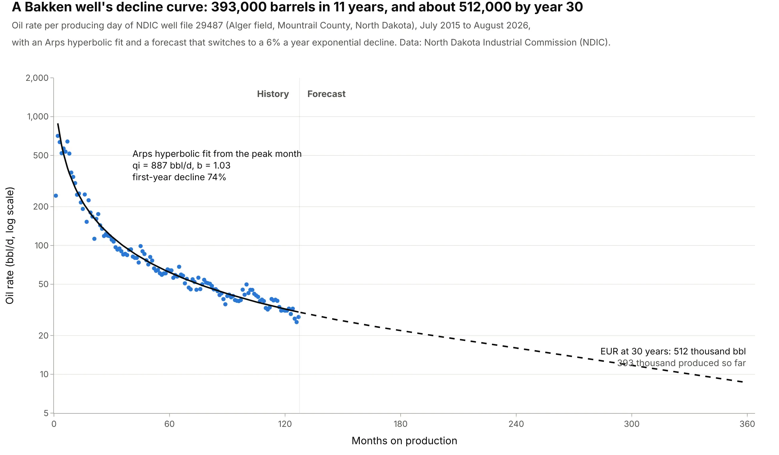
Decline curve of one Bakken shale well in Mountrail County, North Dakota: blue dots of monthly oil rate fall on a log axis from about 700 barrels a day in its second producing month to 28 after 127 months, a black Arps hyperbolic fit runs through them, and a dashed forecast continues to month 360 at about 9 barrels a day, labeled EUR at 30 years 512 thousand barrels, 393 thousand produced so far

Data: North Dakota Industrial Commission (NDIC), monthly well production reports, well file 29487.

How do you read a decline curve? In the example above, notice these things:

Each dot is one month's oil divided by the days the well produced, in barrels per day (bbl/d), against the months it has been producing. The well peaked at 709 bbl/d in its second month and made 27.8 bbl/d in August 2026, eleven years later.
The y axis is logarithmic, so each gridline step is a multiple rather than a fixed amount. That's why the first year, when the rate fell 74%, takes as much room as the next ten.
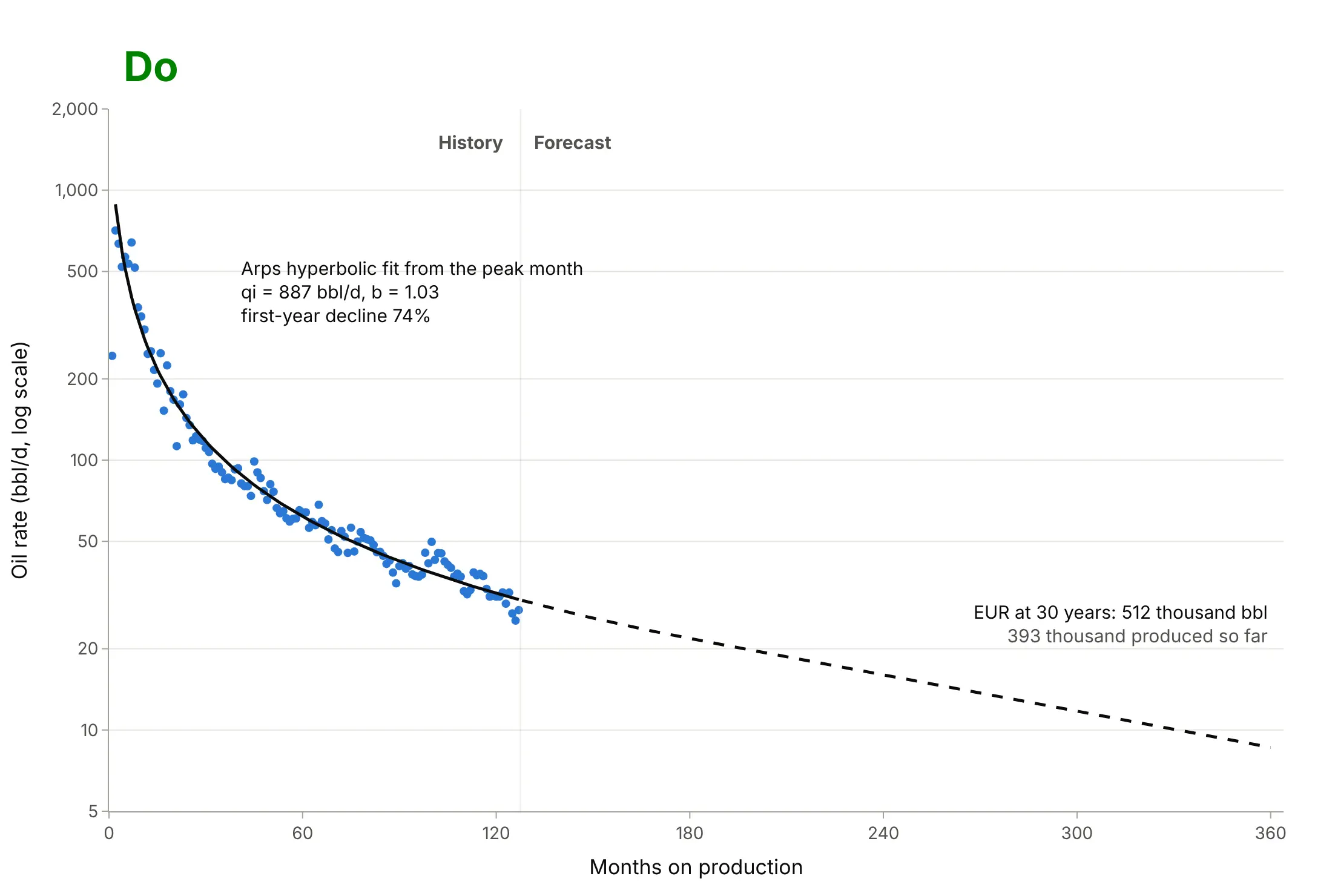
The solid black line is an Arps hyperbolic fit from the peak month, with an initial rate qi of 887 bbl/d and a b factor of 1.03. The b factor sets how fast the decline itself slows down.
The dashed line is the forecast. Adding it to the 393,470 barrels produced so far gives an EUR of about 512,000 barrels at 30 years, so this well has already produced about three quarters of its expected oil.

It's often used for charts like these:

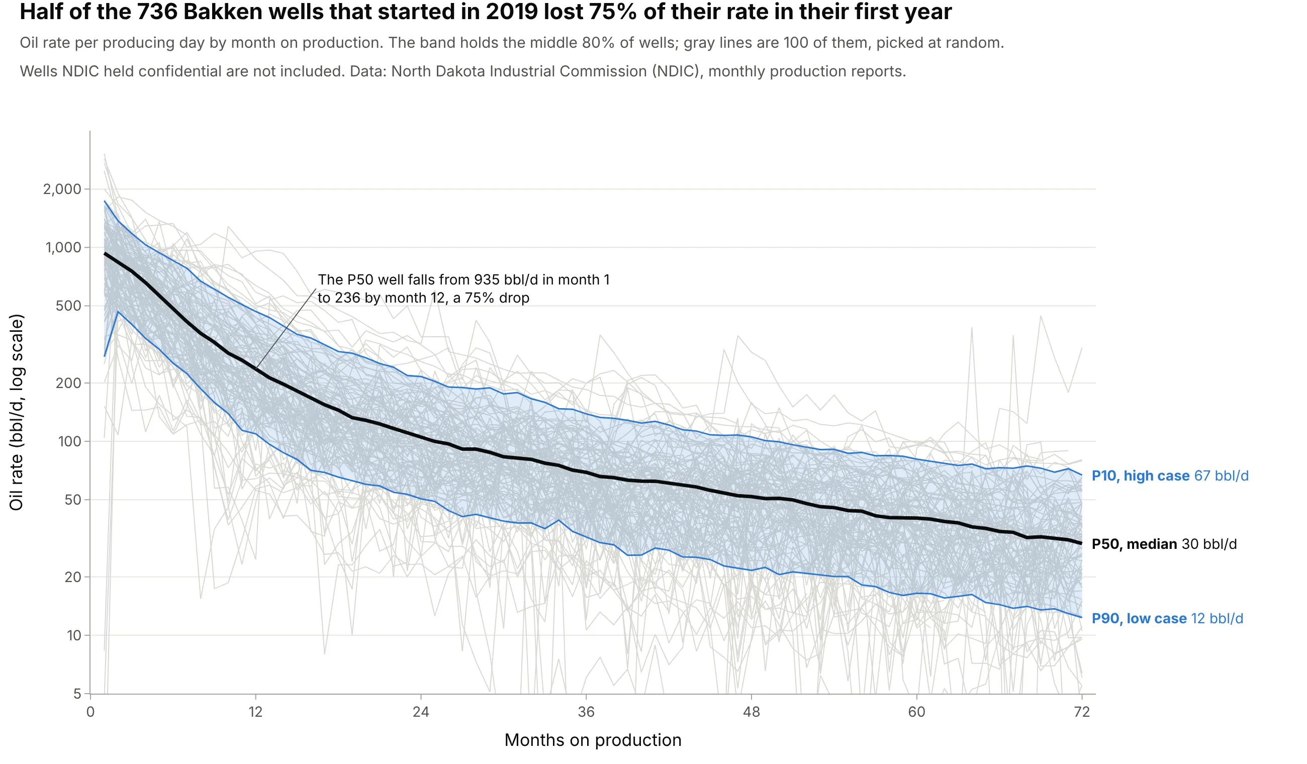
Type curve of 736 North Dakota Bakken wells that started producing in 2019: 100 thin gray well lines, a blue band between P10 and P90 and a bold black P50 line that falls from 935 barrels a day in month 1 to 236 by month 12 and 30 by month 72, where P10 is 67 and P90 is 12

Type curves for planning new wells. Lining up hundreds of wells by month on production turns their decline curves into a P10, P50, and P90 band; the median 2019 Bakken well fell from 935 to 236 bbl/d in its first year. Data: NDIC monthly production reports.

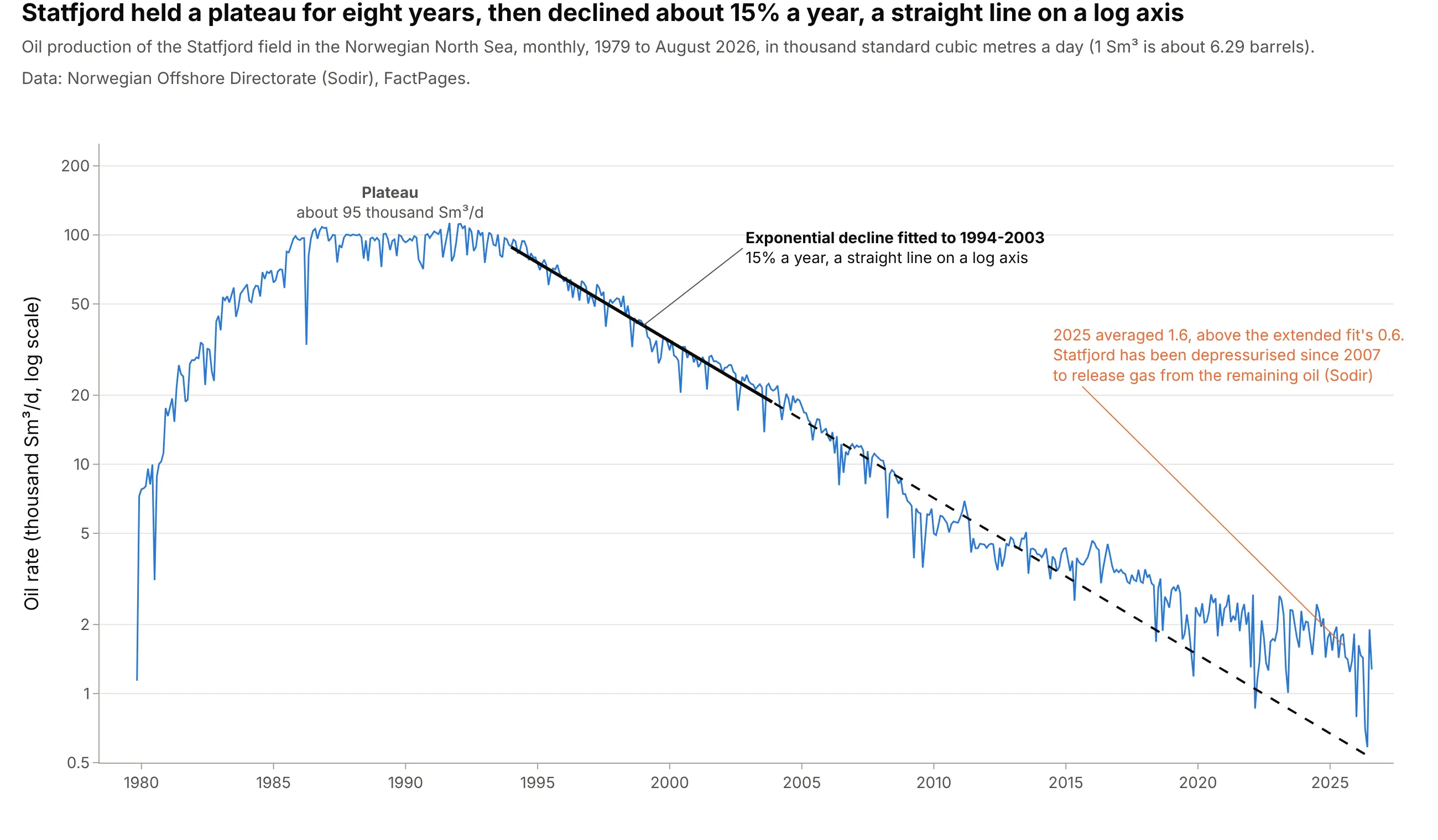
Statfjord field oil rate on a log axis, 1979 to 2026: a build-up, an eight-year plateau near 95 thousand standard cubic metres a day, then a decline that follows a straight black line fitted to 1994-2003 at 15% a year, with the dashed extension below the 2025 rate of 1.6

Field forecasts and reserves, the classic use. Statfjord, Norway's biggest oil field of the 1980s, held a plateau for eight years and then declined about 15% a year, which an exponential decline draws as a straight line on a log axis. Data: Norwegian Offshore Directorate (Sodir), FactPages.

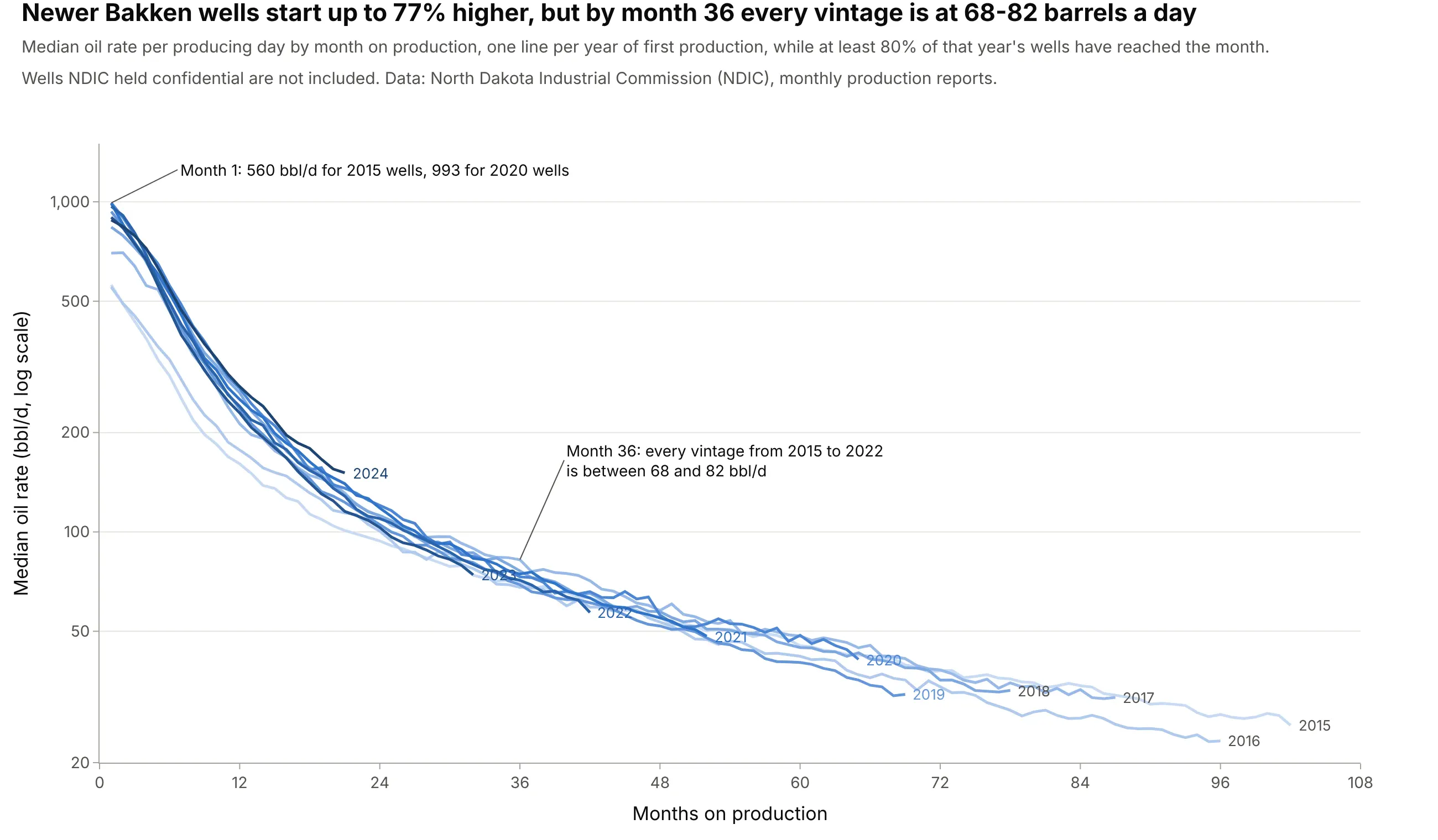
Median oil rate by month on production for Bakken wells of each first-production year from 2015 to 2024 on a log axis: month 1 rises from 560 barrels a day for 2015 wells to 993 for 2020 wells, but by month 36 every vintage from 2015 to 2022 is between 68 and 82

Comparing well designs year by year. Bakken wells that started in 2020 began at a median of 993 bbl/d against 560 for 2015 wells, but by month 36 every year's wells were between 68 and 82 bbl/d. Data: NDIC monthly production reports.

A short history

Petroleum engineers have projected production curves for more than a century. In 1918 J.O. Lewis and Carl Beal of the US Bureau of Mines described the "production curve method," in which a well's past production is plotted and "projected from the terminal to the point representing the minimum production to which the well can be pumped with profit", along with average, maximum, and minimum "appraisal curves" for whole fields in Oklahoma, an early version of today's P10-P90 band. They also recommended logarithmic paper, because "many production records of individual wells ... can be made to approach straight lines" on it (Lewis and Beal 1918). In 1945 J.J. Arps, building on that work and on later papers such as Cutler's of 1924, published the exponential, hyperbolic, and harmonic equations still in use (Arps 1945), and in 1980 M.J. Fetkovich tied them to reservoir flow with type curves (Fetkovich 1980). Shale wells, with their long early declines and b factors above 1, led to modified forecasts and new models from 2008 on (Ilk et al. 2008, Duong 2011).

How decline curve analysis works

A decline curve is a chart and a model at the same time. The chart shows what a well has done; the model, almost always one of Arps's equations, says what it will do. These are the ideas behind both, in the order an engineer uses them.

Why the rate axis is logarithmic

A well's rate falls by a share of itself each month, not by a fixed amount, so on a linear axis the first year fills the chart and the next ten years are squashed against the bottom. On a log axis every halving takes the same height, and a constant percentage decline is a straight line:

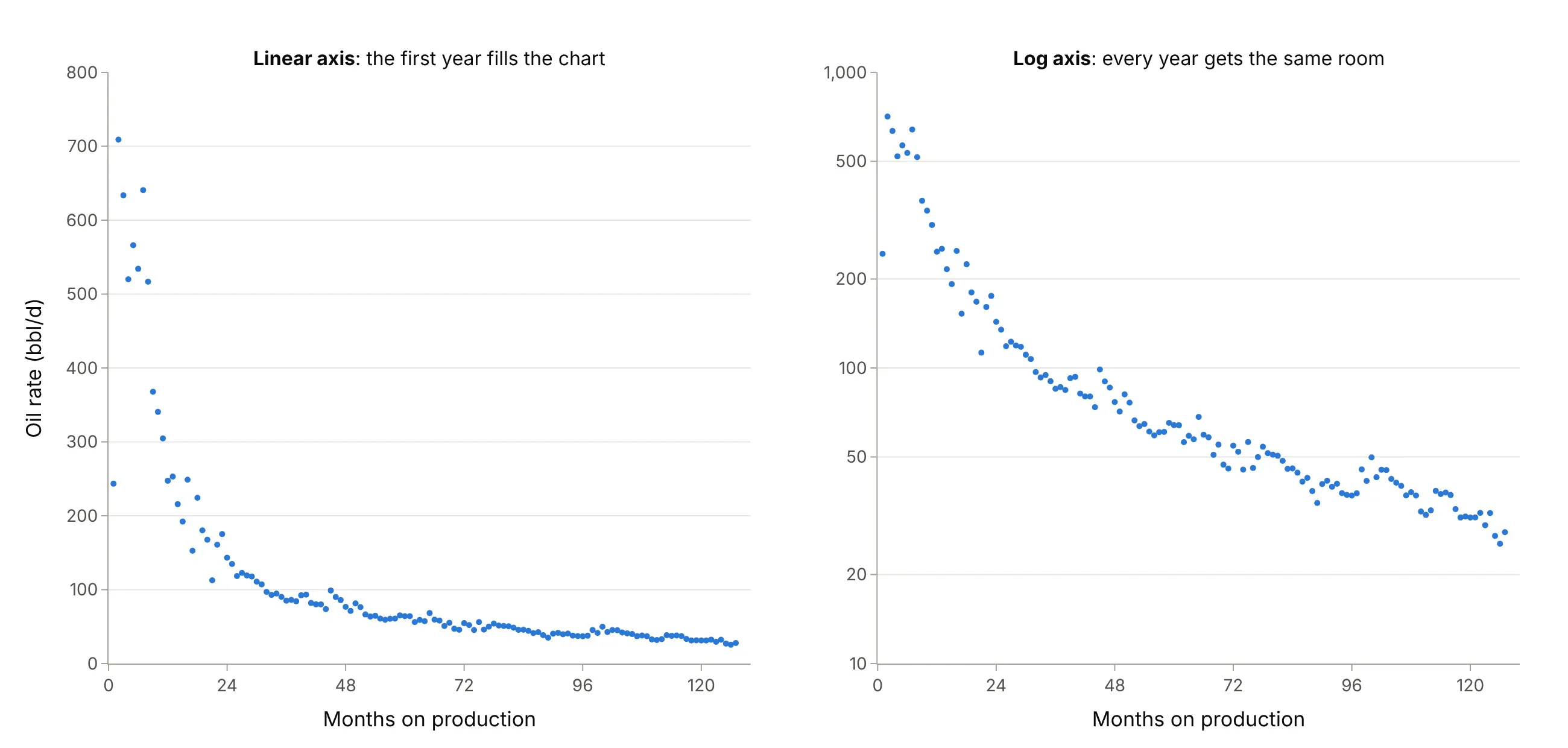
The main well's monthly rates drawn twice: on a linear axis from 0 to 800 barrels a day the first year's points tower over a flat line near the bottom, and on a log axis from 10 to 1,000 the same points form an even, readable curve across eleven years

Data: NDIC monthly production reports, well file 29487.

Arps's three declines and the b factor

The decline rate D is the share of the rate a well loses per unit of time. Arps's equation gives the rate q at time t from three numbers, the initial rate qi, the initial decline Di, and the exponent b:

q(t) = qi / (1 + b × Di × t)^(1/b)

With b = 0 the decline rate never changes, which is an exponential decline: q(t) = qi × e^(−Di × t), a straight line on a log axis. With b = 1 the decline rate falls in proportion to the rate, a harmonic decline. Values between 0 and 1 are hyperbolic. The IHS Harmony decline analysis reference lists the cumulative-production versions of each. Here are four values of b with the same start:

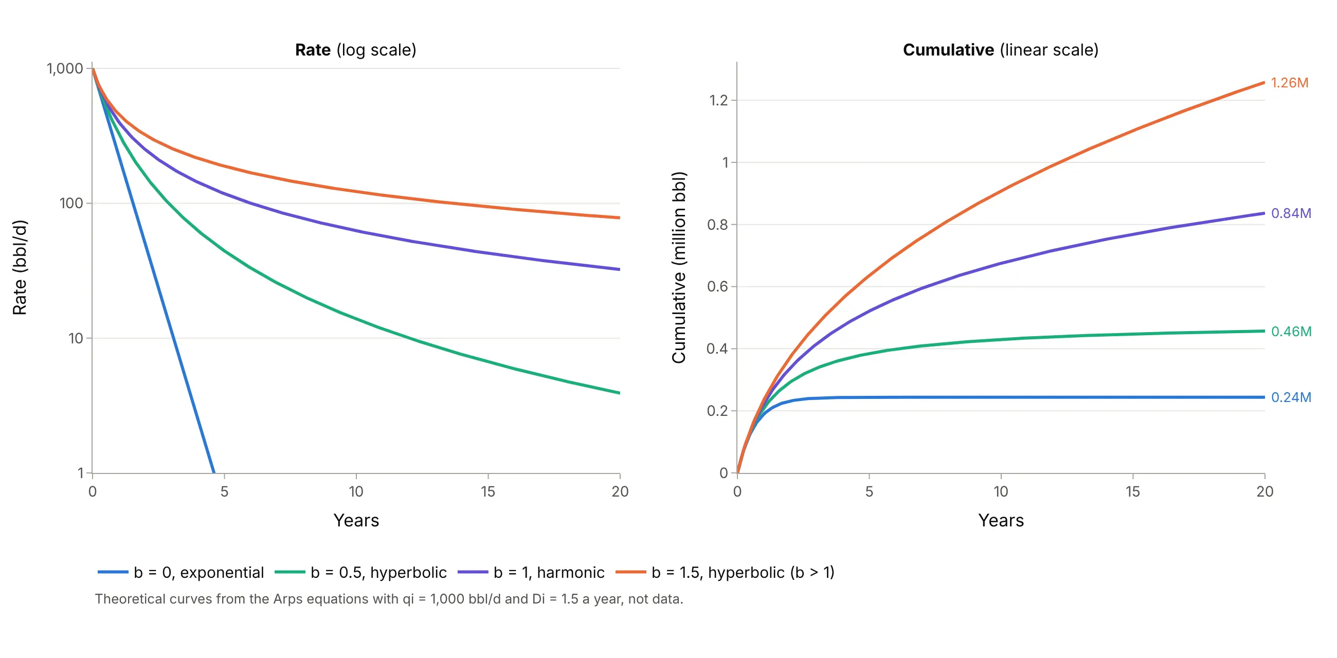
Four theoretical Arps curves with the same initial rate of 1,000 barrels a day and initial decline of 1.5 a year: on a log rate axis b = 0 is a straight line that drops below 1 barrel a day by year 5, while b = 0.5, 1 and 1.5 flatten more and more; on a linear cumulative axis their 20-year totals are 0.24, 0.46, 0.84 and 1.26 million barrels

Data: theoretical curves from the Arps equations, not data.

The curves start together and end far apart: after 20 years the b = 1.5 curve has produced more than five times as much as the exponential one. That's why the b factor matters more than any other number in a decline forecast.

Fitting the curve

To fit Arps to a well, take the months from the peak on (the ramp-up before it isn't decline) and find the qi, Di, and b that minimize the error in log rate, which scipy.optimize.curve_fit does in a few lines. On the main well, an exponential decline misses badly, while harmonic and hyperbolic fits are equally good:

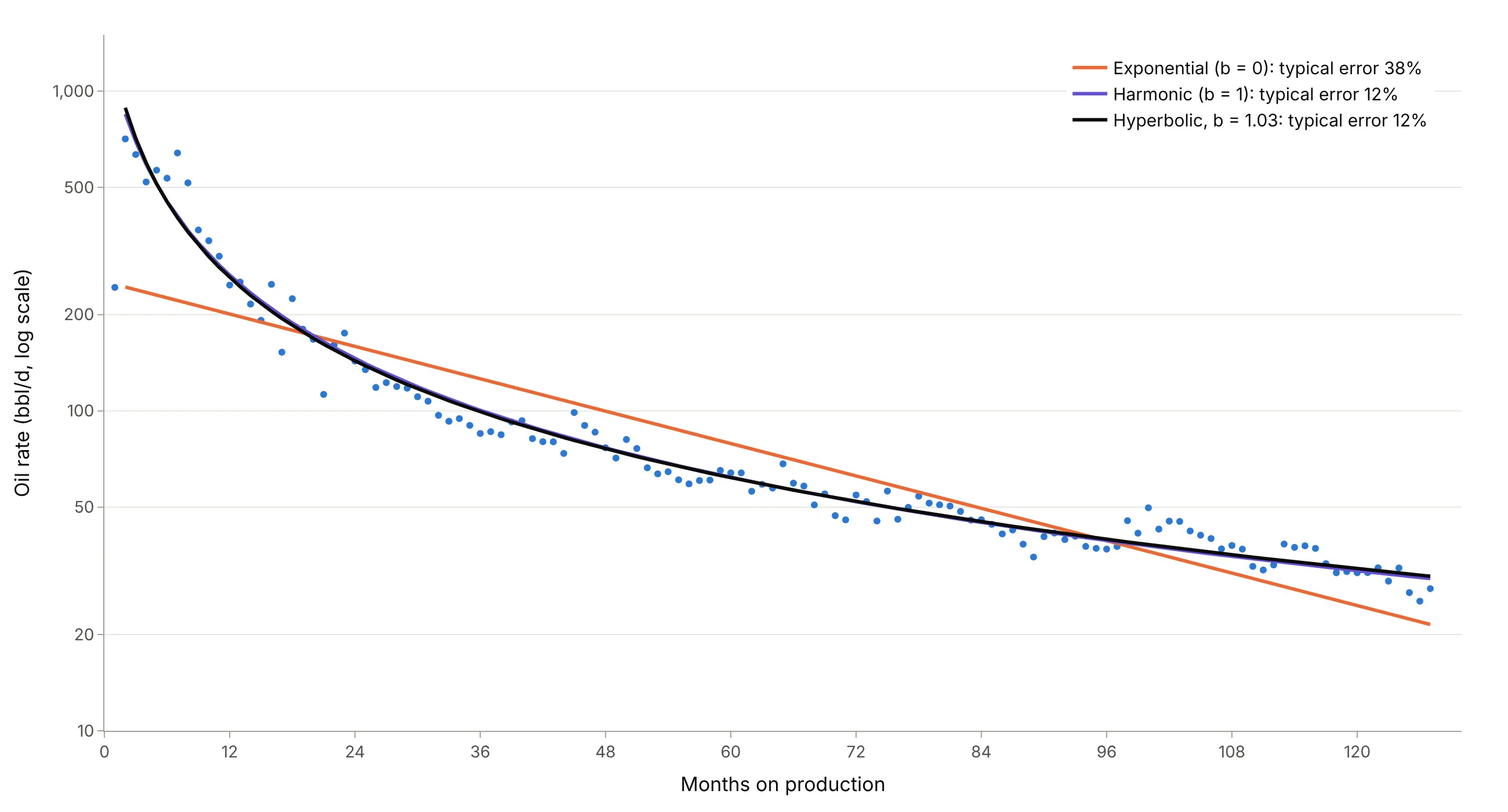
The main well's monthly rates on a log axis with three fitted lines: a straight orange exponential that starts far below the early months and ends below the late ones, with a typical error of 38%, and almost identical purple harmonic and black hyperbolic curves with b = 1.03 that follow the points, each with a typical error of 12%

Data: NDIC monthly production reports, well file 29487. Typical error is the root mean square error of log rate, as a percentage.

From rate to EUR, and why forecasts need a terminal decline

The area under the rate curve is cumulative production, and the cumulative at the end of the forecast is the estimated ultimate recovery (EUR). With b of 1 or more the area never stops growing, so in theory a well would produce forever. The IHS reference notes that extending hyperbolic declines over long periods "frequently results in unrealistically high reserves", and the usual fix, the modified hyperbolic, switches to an exponential decline once the hyperbolic decline rate falls to a set floor. This guide uses 6% a year, an assumption for illustration:

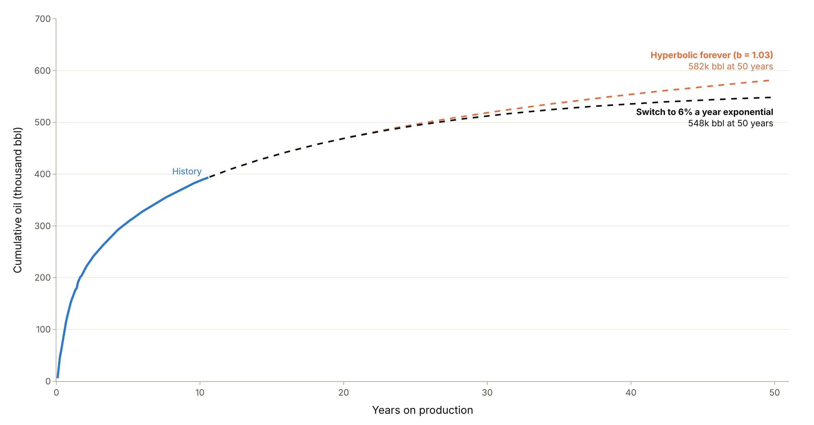
Cumulative oil of the main well over 50 years: the blue history reaches 393 thousand barrels after about 11 years, a dashed orange hyperbolic forecast that never switches reaches 582 thousand at 50 years, and a dashed black forecast that switches to a 6% a year exponential decline reaches 548 thousand

Data: NDIC monthly production reports, well file 29487.

For this well b is close to 1, so the switch changes the 50-year total by 34,000 barrels. For a well with b of 1.5 or more, the difference is much larger, which is why reserves evaluators state the terminal decline they use.

Type curves and P10, P50, and P90

One well's curve says little about the next well. A type curve lines up many wells by month on production and shows the spread at each month. Oil and gas use the convention of the Society of Petroleum Engineers (SPE) Petroleum Resources Management System (PRMS 2018): P90 is the low estimate, which has at least a 90% probability of being met or exceeded, P50 the best estimate, and P10 the high estimate. So P90 is the bottom of the band and P10 the top, the opposite of how a statistician reads percentiles. In the 2019 Bakken type curve above, P10 is 67 bbl/d and P90 is 12 bbl/d at month 72. Here months on production count only months with at least 15 producing days, so shut-ins don't pull the curve down, and the rate is per producing day.

Why shale wells decline so steeply

Arps's curves describe boundary-dominated flow, the stage after the pressure drop around a well has reached the edges of the rock it drains. In conventional reservoirs that takes days, but in rock so tight that it needs "extensive fracture networks", the early transient flow "could last for several years" (IHS). Shale wells such as those in North Dakota's Bakken formation are long horizontal wells with many hydraulic fractures, so they produce fast from the rock next to the fractures and then fall off, and while the flow is still transient their fits give b above 1. In our data a third of Bakken wells fit b above 1, and the median 2019 well produced 57% of its first six years of oil in year one.

Alternatives to a decline curve

Here's the same well drawn six ways. Some are better for the question, some worse, some just different:

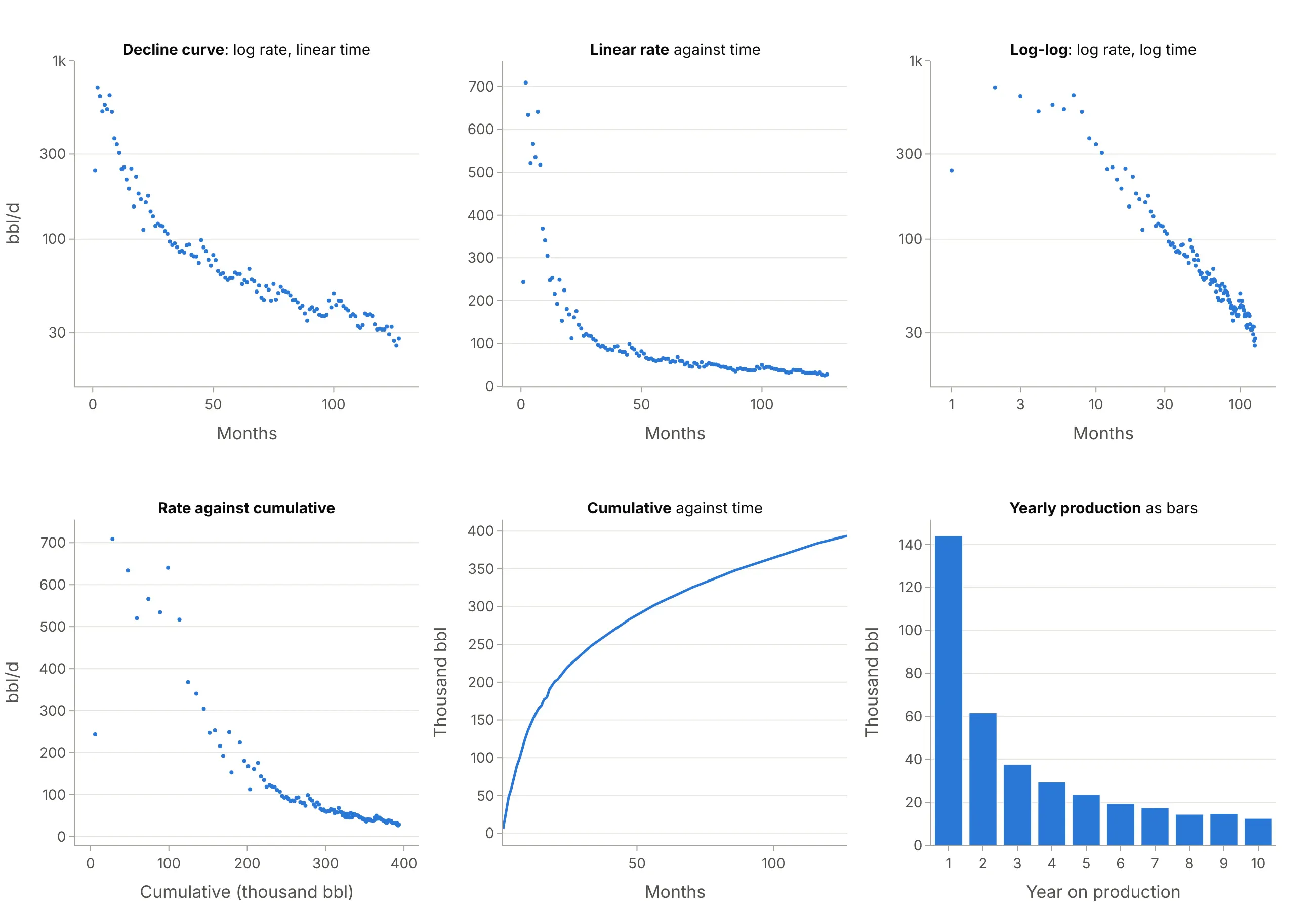
The main well drawn six ways: a decline curve with a log rate axis, the same rates on a linear axis where everything after year 2 is flat near zero, a log-log plot where the points bend down, rate against cumulative production, cumulative production against time rising and flattening toward 393 thousand barrels, and yearly production as ten bars falling from 144 to 12 thousand barrels

Linear rate axis (worse). The first year fills the chart, so the decline after the second year, which holds most of the forecast, is a flat line near zero.
Log-log plot (different, for diagnosing flow). Log time spreads out the first months, and engineers use its slopes to identify flow regimes before fitting.
Rate against cumulative (works too). An exponential decline is a straight line that hits zero at the EUR, so the reserves can be read off the x axis. Example 1 below does this for Statfjord.
Cumulative against time (better for volumes). It shows barrels directly and is smooth, which is why type curves are often shown this way (example 6 below), but the shape of the decline is harder to see.
Yearly bars, a bar chart (works too, for reports). The first year at 144,000 barrels and the tenth at 12,000 are easy to compare, but you can't fit or extend a curve on them.

Comparing many wells needs small multiples of decline curves (example 2 below), and the spread of EURs or b factors across a field is a histogram or an ECDF plot (example 3).

How to make a decline curve

With AI

ChatGPT, Claude Code, GitHub Copilot, Cursor, and other AI tools are excellent at writing Plotly code. Name Plotly in the prompt, and say which months to fit, which Arps model to use, and how to end the forecast:

Make a plotly decline curve from well.csv (columns: date, pmonth, days, oil_bbl, rate; one row per month).

- Oil rate per producing day as dots against producing month, on a log y axis with units in the title.
- Fit an Arps hyperbolic q = qi / (1 + b Di t)^(1/b) with scipy curve_fit on log(rate), from the peak month.
- Forecast to month 360, switching to a 6% a year exponential decline when the decline falls to that rate.
- History solid, forecast dashed, and the EUR (cumulative to date plus the forecast) labeled at the end.
- Check: print qi, Di, b, the first-year decline, and the EUR.

With Plotly Studio

Plotly Studio is a desktop app where you point an AI at a dataset and it builds charts and a Dash app around your questions. Ask for a decline curve the same way:

Show a decline curve of oil rate by months on production for the selected well on a log axis, with an Arps hyperbolic fit and a 30-year forecast, the EUR and b factor in the title, and a dropdown to pick the well.

Make a decline curve in Python or JavaScript

This is the code AI tools write under the hood. Plotly has no dedicated decline curve trace, so a decline curve is a go.Scatter of the rates on a log y axis plus a second go.Scatter for the fitted Arps curve. This helper fits the curve with SciPy and returns a go.Figure, and every example in this guide builds on the same idea:

import numpy as np
import pandas as pd
import plotly.graph_objects as go
from scipy.optimize import curve_fit


def arps(t, qi, di, b):
    """Arps hyperbolic decline: rate at time t (years), initial rate qi, initial decline di (1/year), exponent b."""
    return qi / (1 + b * di * t) ** (1 / b)


def decline_curve(months, rate, horizon=360):
    """Fit Arps to monthly rates from the peak month and draw history, fit, and forecast on a log axis."""
    months, rate = np.asarray(months, float), np.asarray(rate, float)
    pk = rate[:3].argmax()  # fit from the peak, not the ramp-up
    t, q = (months[pk:] - months[pk]) / 12, rate[pk:]
    (qi, di, b), _ = curve_fit(lambda t, qi, di, b: np.log(arps(t, qi, di, b)), t, np.log(q),
                               p0=[q[0], 2, 1], bounds=([0, 0.01, 0.01], [1e5, 50, 2.5]))
    tf = np.arange(months[pk], horizon + 1)
    qf = arps((tf - months[pk]) / 12, qi, di, b)
    fig = go.Figure([
        go.Scatter(x=months, y=rate, mode="markers", name="History"),
        go.Scatter(x=tf, y=qf, mode="lines", line_dash="dash", name=f"Arps fit, b = {b:.2f}"),
    ])
    fig.update_yaxes(type="log", title="Oil rate (bbl/d)")
    fig.update_xaxes(title="Months on production")
    return fig


df = pd.read_csv("well.csv").dropna(subset=["pmonth"])  # one row per producing month: pmonth, rate
fig = decline_curve(df.pmonth, df.rate)
fig.show()

For the terminal decline, switch the forecast to q_sw * np.exp(-dn * (t - t_sw)) from the time t_sw when the hyperbolic decline di / (1 + b * di * t) falls to dn = -np.log(1 - 0.06). For a type curve, pivot the wells to one column per well and draw df.quantile(0.9, axis=1) (P10), the median and quantile(0.1) (P90) with fill="tonexty" between them.

In JavaScript, plotly.js draws the same chart from the rates and the fitted parameters:

<div id="chart"></div>
<script src="https://cdn.plot.ly/plotly-4.1.1.min.js"></script>
<script>
  // Oil rate (bbl/d) of a Bakken well in its first 36 producing months (NDIC file 29487)
  const rate = [243, 709, 634, 520, 566, 534, 641, 517, 368, 341, 305, 247, 253, 216, 192, 249, 153, 224,
                180, 168, 113, 161, 175, 143, 135, 118, 123, 119, 118, 111, 107, 97, 93, 95, 90, 85];
  const months = rate.map((_, i) => i + 1);

  // Arps hyperbolic decline fitted to this well's full history (in Python): qi, Di per year, b
  const qi = 887, di = 2.94, b = 1.03;
  const tf = Array.from({length: 359}, (_, i) => i + 2);  // from the peak month (2) to month 360
  const qf = tf.map(m => qi / Math.pow(1 + b * di * (m - 2) / 12, 1 / b));

  Plotly.newPlot("chart", [
    {x: months, y: rate, mode: "markers", name: "History", marker: {color: "#2a78d6"}},
    {x: tf, y: qf, mode: "lines", name: "Arps fit and forecast", line: {color: "#0b0b0b", dash: "dash"}}
  ], {
    width: 900, height: 500,
    xaxis: {title: {text: "Months on production"}},
    yaxis: {title: {text: "Oil rate (bbl/d)"}, type: "log"}
  });
</script>

Share it

Every Plotly chart has a Share chart button (the cloud icon in its toolbar) that uploads it to Plotly Cloud and gives you a link. Only you can see it until you change its visibility.

For a live app, put the chart in a Dash app and publish it with the Plotly Cloud command-line interface (CLI). Coding agents can run these commands for you:

pip install "dash[cloud]"
plotly user login
plotly app publish

If your data has to stay in your own cloud or data center, publish to Dash Enterprise instead.

Dos and don'ts

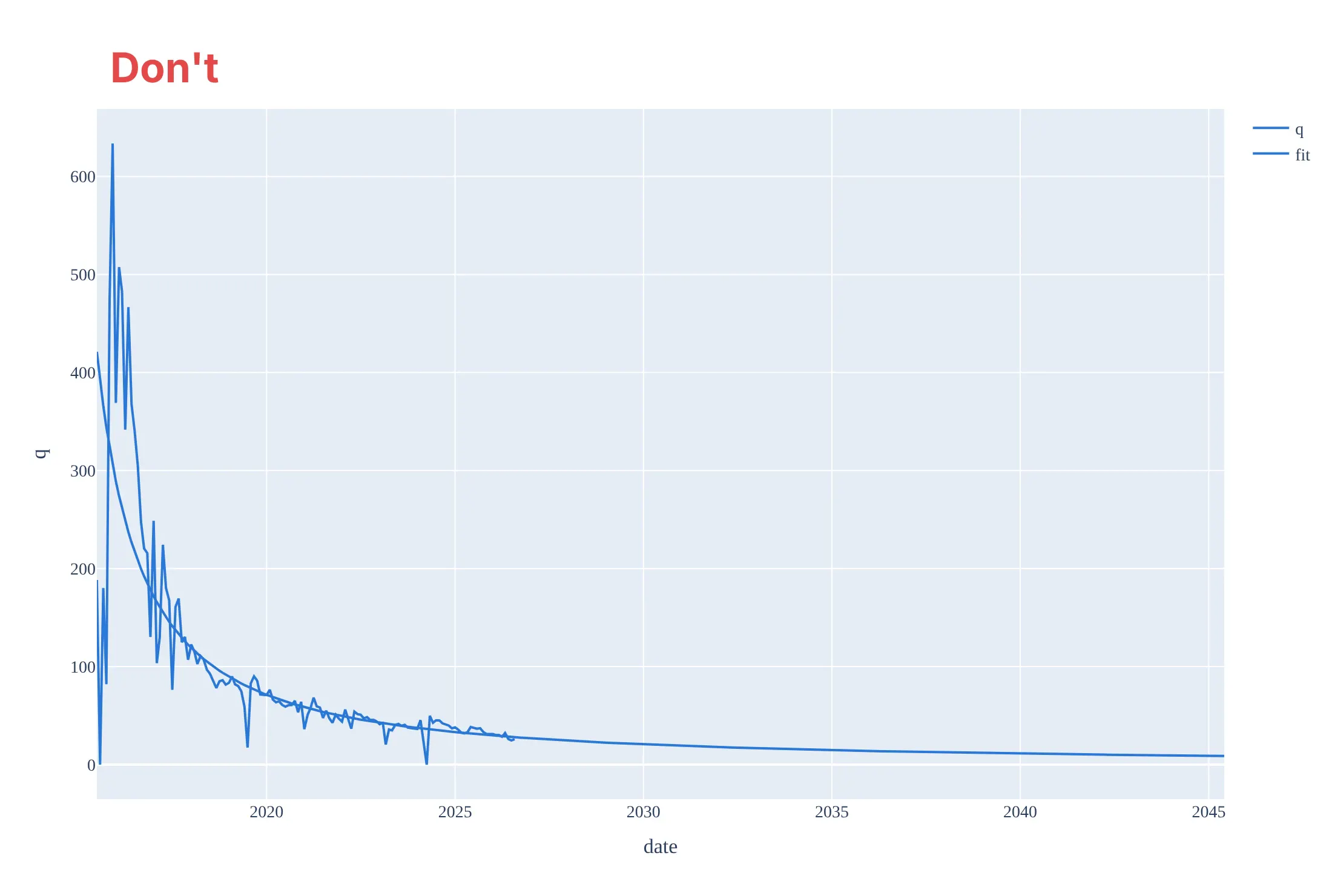
Most of the work in a decline curve is choosing which months to fit and making the forecast look like a forecast. Here is the main well both ways, in the same blue.

Don't plot calendar-day rates by date on a linear axis, which shows the shut-in months as drops to zero and squashes ten years against the bottom, fit through the ramp-up month and the shut-ins (which gives an initial rate of 421 bbl/d where the well made 709), draw the history and the 30-year forecast as two identical lines, or keep raw column names, a default legend and a serif font:

The main well as a blue line by calendar date on a linear axis to 2045, with drops to zero for shut-in months, a fitted curve in the same blue that starts at 421 under the early peak and runs on to 2045 without any change of style, a legend reading q and fit, axis titles date and q, and a serif font

Do plot the rate per producing day by producing month on a log axis, fit from the peak month, draw the history as dots, the fit solid, and the forecast dashed, and label the fitted values and the EUR:

The same well as dots on a log axis by month on production, with a solid black hyperbolic fit, a dashed forecast to month 360 after a line marking history and forecast, the fitted qi of 887, b of 1.03 and first-year decline of 74% in a label, and the EUR at 30 years of 512 thousand barrels

Checklist

Use a log rate axis and put the units in the axis title: bbl/d, mcf/d (thousand cubic feet of gas a day), or thousand Sm³/d (standard cubic metres a day, the unit Norway reports in).
Fit from the peak month and leave out shut-ins and partial months, or count only producing months.
Draw the forecast differently from the history, and say where it switches to a terminal decline.
State qi, b, the decline, and the EUR with the assumptions that produced them (horizon, terminal decline, and economic limit).
Label P10 as the high case and P90 as the low case on type curves, and say how many wells each month includes.

Don't

Extend a hyperbolic fit with b of 1 or more without a terminal decline.
Fit across a change in how the well or field is produced, such as a refracture or the start of water injection (example 7 below).
Average wells of different ages by calendar date; line them up by month on production.
Present a type curve built only from the best wells, or from wells that are missing their first months, as the typical well.

Options to customize

A decline curve in Plotly is a scatter trace on a log axis plus fitted lines, so these are the options that matter most. The full lists are in the scatter trace reference, the log axes documentation and the SciPy curve_fit documentation.

fig.update_yaxes(type="log"): the log rate axis; set range in log10 units, for example [0.7, 3.3] for 5 to 2,000.
tickvals, ticktext: 10, 20, 50, 100, and so on instead of Plotly's default log ticks.
go.Scatter(mode="markers"): monthly history as dots, so the fitted line stays visible.
line_dash="dash": the forecast, so nobody mistakes it for measured production.
fig.add_vline: the last month of history, or an event such as the start of water injection.
fill="tonexty": the band between P10 and P90 on a type curve.
make_subplots(rows=..., cols=..., shared_yaxes=True) or px.line(..., facet_col=...): small multiples of many wells on the same axes.
customdata and hovertemplate: the calendar month, producing days, or well name on hover.
x=None gaps in one trace or go.Scattergl: hundreds or thousands of wells as one trace (see the FAQ).
scipy.optimize.curve_fit(..., bounds=...): keep b between 0 and a sensible maximum (2.5 here) and fit log rate, not rate.

More decline curve examples

Seven more decline curves built from real public data, each with its source, the technique that makes it work, and a prompt to rebuild it. They cover Norway's offshore fields and North Dakota's shale wells.

1. Rate against cumulative: Statfjord's straight line to its EUR

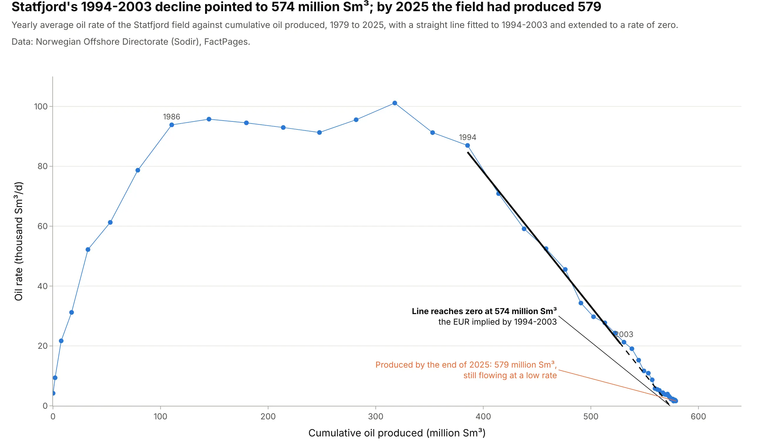
Statfjord's yearly average oil rate against cumulative oil produced on linear axes: a rise, a plateau near 95 thousand Sm³ a day, then points from 1994 falling along a straight black line fitted to 1994-2003 that reaches zero at 574 million Sm³, next to the 579 million actually produced by the end of 2025

An exponential decline is a straight line when rate is plotted against cumulative production, so extending it to zero reads off the EUR. Fitted to 1994-2003, Statfjord's line reached zero at 574 million standard cubic metres (Sm³); by the end of 2025 the field had produced 579 million. Data: Norwegian Offshore Directorate (Sodir), FactPages, field production monthly.

Tip: use linear axes on a rate-cumulative plot, so the straight line and its intercept can be read directly.

Get the data from the Norwegian Offshore Directorate's FactPages (factpages.sodir.no, table field_production_monthly,
net oil in million Sm3 by field and month) and shape it into a yearly table for STATFJORD (columns: year, oil_msm3,
rate_ksm3d, cum_msm3).

Build a plotly scatter of rate against cumulative, fit a straight line to 1994-2003 with numpy polyfit, extend it
dashed to a rate of zero, and label the EUR and the cumulative produced by 2025.

2. Twelve Bakken wells, twelve fits (small multiples)

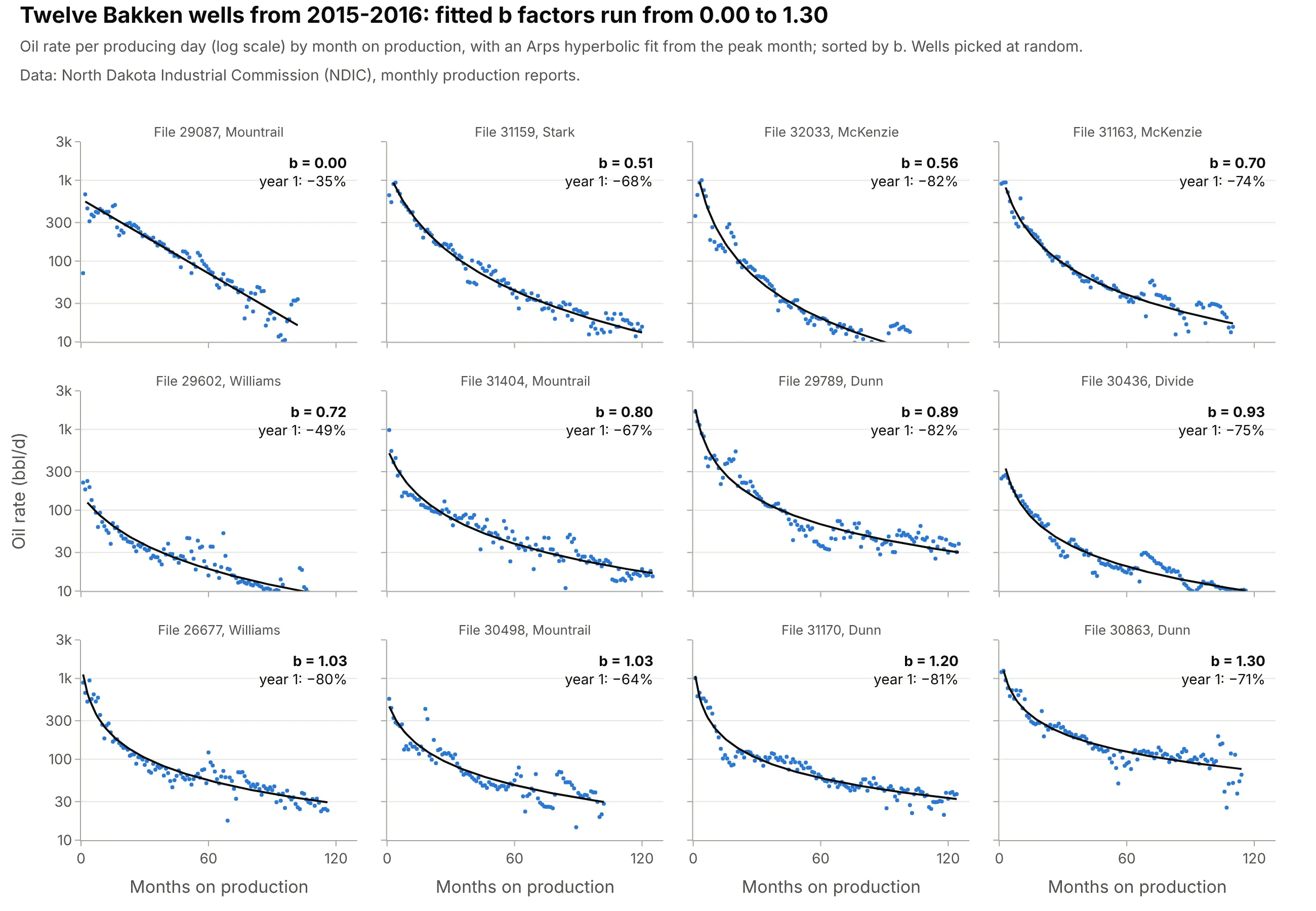
Twelve small decline curves of Bakken wells from 2015-2016, each with blue monthly dots and a black Arps fit on shared log axes, sorted by fitted b from 0.00 to 1.30, with first-year declines between 35% and 82%

Twelve wells picked at random from the same play fit b factors from 0.00 to 1.30 and first-year declines from 35% to 82%, which is why engineers check fits well by well before building a type curve. Data: NDIC monthly production reports.

Tip: share both axes and sort the panels by the fitted parameter, so the differences in shape are the only thing that changes.

Get the data from the North Dakota Industrial Commission's monthly production reports (dmr.nd.gov/oilgas, one Excel
file per month with oil, gas, water and producing days per well) and shape it into a table of 12 Bakken wells
(columns: well, pmonth, rate).

Build plotly small multiples with make_subplots (3 x 4, shared log y axis), an Arps hyperbolic fit from scipy
curve_fit in each panel, b and the first-year decline in the corner, sorted by b.

3. A third of Bakken wells fit b above 1

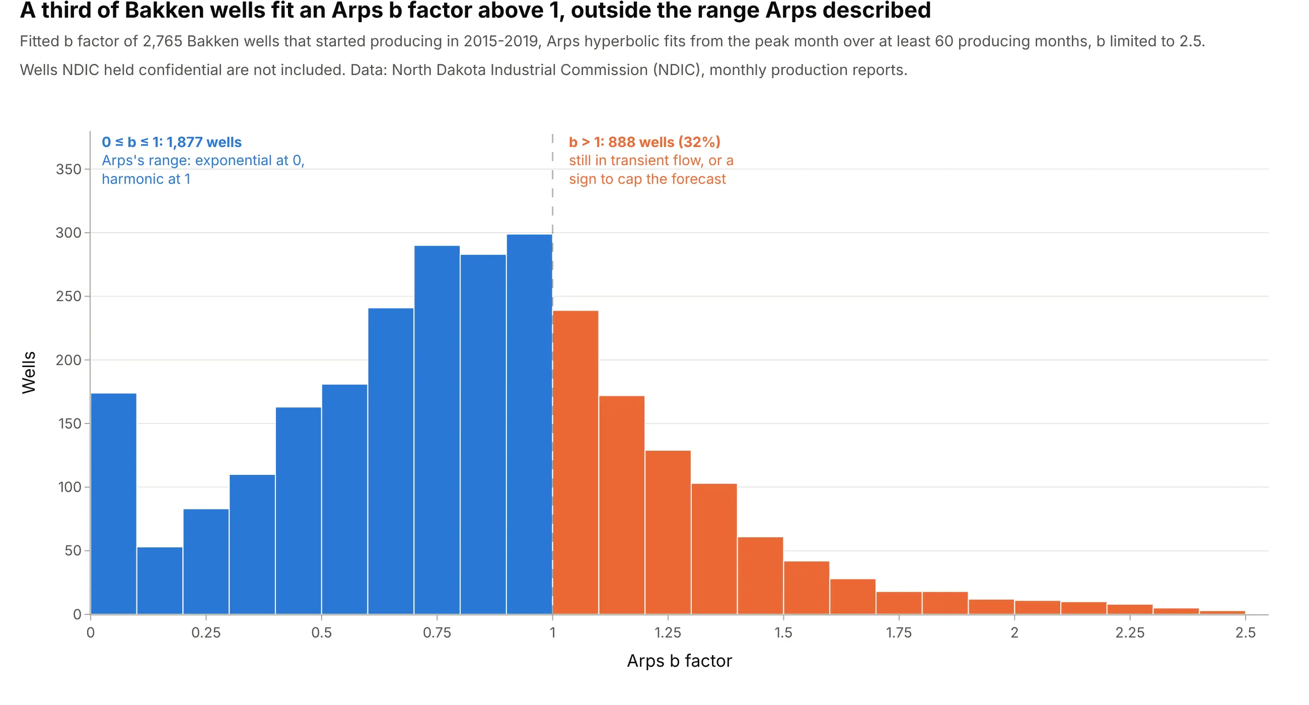
Histogram of the fitted Arps b factor of 2,765 Bakken wells: blue bars from 0 to 1 holding 1,877 wells with a peak near 0.8 to 1, and orange bars above 1 holding 888 wells, 32%, in a tail to 2.5, with a dashed line at b = 1

Of 2,765 Bakken wells that started in 2015-2019, 888 (32%) fit an Arps b factor above 1, outside the 0 to 1 range of Arps's theory, and the median is 0.83. Values above 1 often mean the well is still in transient flow, so the forecast needs a terminal decline. Data: NDIC monthly production reports.

Tip: split the histogram at the threshold that changes the decision (here b = 1) and color the two sides.

Get the data from the North Dakota Industrial Commission's monthly production reports (dmr.nd.gov/oilgas, monthly
Excel files) and fit an Arps hyperbolic to every Bakken well with first oil in 2015-2019 and 60 producing months,
into a table (columns: well, first_year, qi, di, b).

Build a plotly histogram of b with bins of 0.1, wells above 1 in a second color, a dashed line at 1, and the count
and share on each side.

4. Oil, gas, and water from the same well

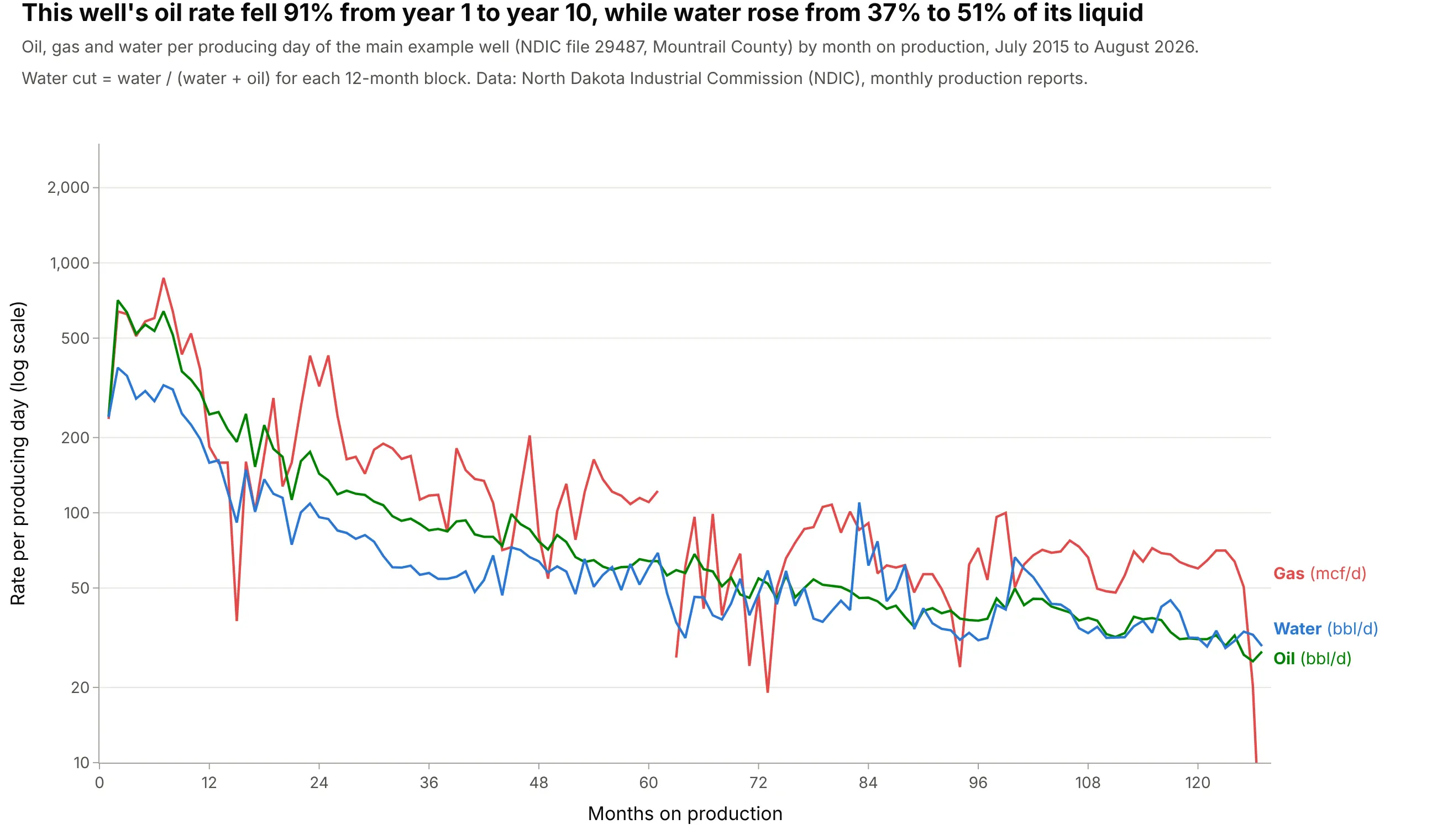
Oil, gas and water per producing day of the main well on one log axis by month on production: green oil and blue water fall from about 700 and 380 to about 30 each, red gas is noisier, and the oil falls 91% from year 1 to year 10 while water rises from 37% to 51% of the liquid

The main well's oil fell 91% from its first year to its tenth, while water rose from 37% to 51% of the liquid it produced. Water and gas cost money to handle, so engineers read the three streams together. Data: NDIC monthly production reports, well file 29487.

Tip: put all three streams on one log axis with direct labels, so their ratios read as vertical gaps.

Get the data from the North Dakota Industrial Commission's monthly production reports (dmr.nd.gov/oilgas, monthly
Excel files) for well file 29487 and shape it into a table (columns: pmonth, days, oil_bbl, gas_mcf, water_bbl).

Build a plotly line chart of oil (bbl/d), gas (mcf/d) and water (bbl/d) per producing day on one log y axis, each
labeled at its right end, and print the water cut by year.

5. A cumulative type curve: most of the oil comes in year one

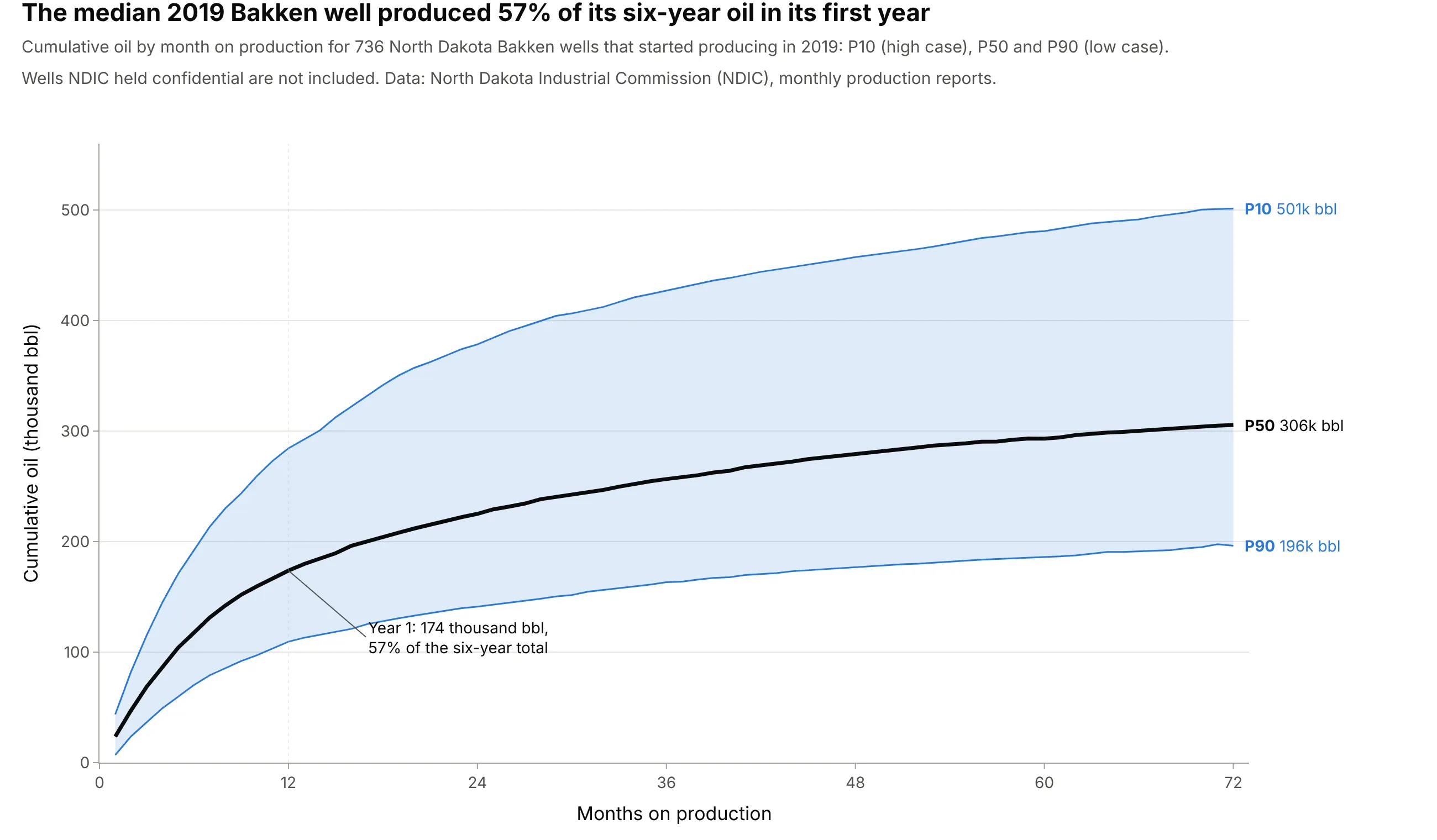
Cumulative oil by month on production for 736 Bakken wells from 2019: a blue band from P90 at 196 thousand barrels to P10 at 501 thousand at month 72, and a black P50 that reaches 174 thousand by month 12, 57% of its 306 thousand at month 72

The median 2019 Bakken well produced 174,000 barrels in its first year, 57% of the 306,000 it made in six years. Cumulative type curves are smooth and read directly in barrels, which is what reserves and economics use. Data: NDIC monthly production reports.

Tip: mark the first year with a dotted line and say what share of the total it holds.

Get the data from the North Dakota Industrial Commission's monthly production reports (dmr.nd.gov/oilgas, monthly
Excel files) and shape the 2019 Bakken wells into a table of cumulative oil by producing month (columns: well,
pmonth, cum_bbl).

Build a plotly type curve of P10 (90th percentile), P50 and P90 (10th percentile) cumulative oil with the band
filled, labeled at month 72, and the P50's year-one share annotated.

6. Norway's 12 biggest fields, normalized to their peak

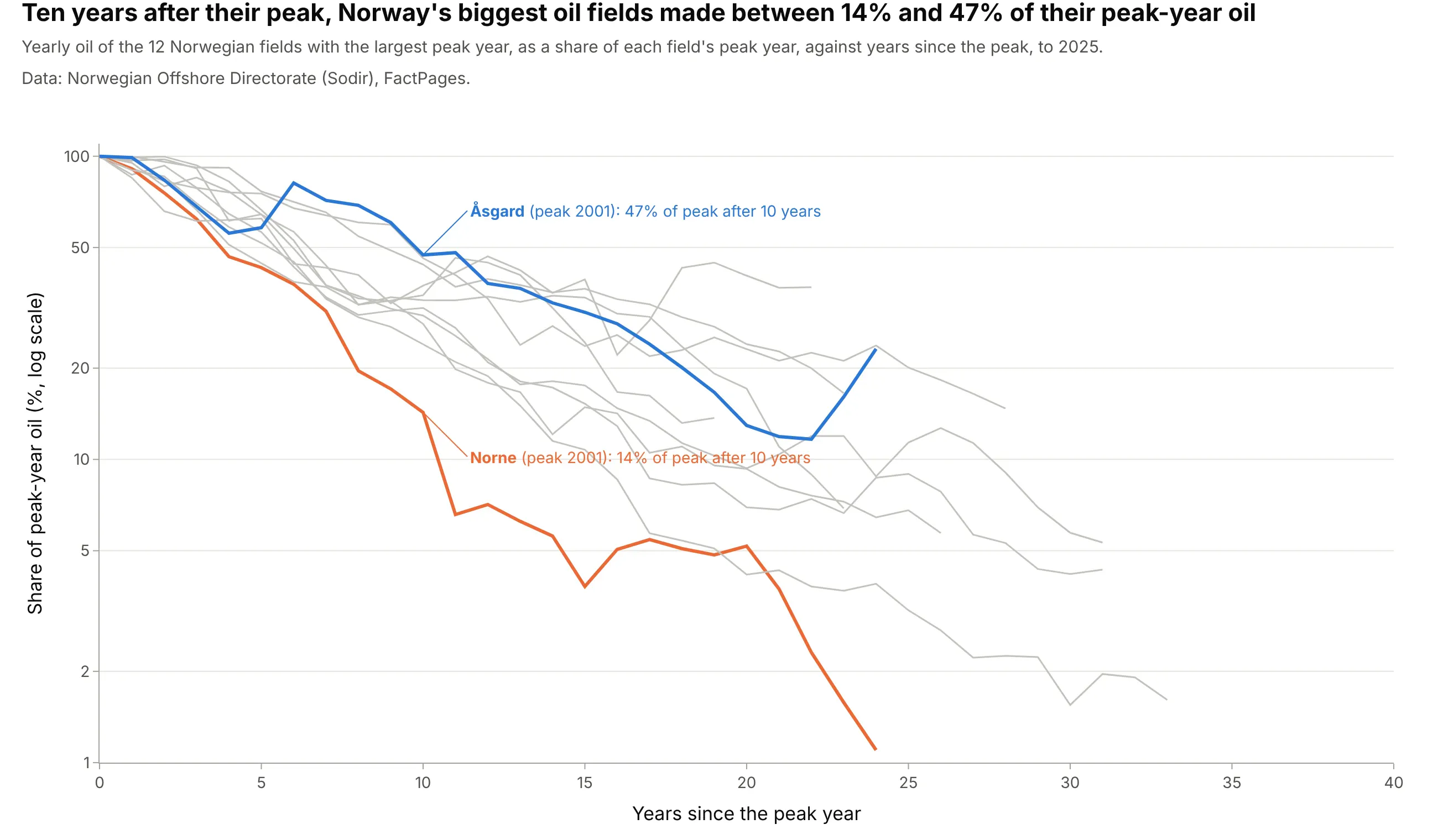
Yearly oil of Norway's 12 largest fields as a share of each field's peak year against years since the peak on a log axis: gray lines fall at different speeds, Norne in orange falls to 14% of its peak after 10 years and Åsgard in blue holds 47%

Ten years after their peak year, Norway's biggest oil fields produced between 14% (Norne) and 47% (Åsgard) of their peak-year oil. Dividing each field by its own peak lines up fields of very different size, the field-level cousin of a type curve. Data: Sodir FactPages, field production monthly.

Tip: normalize to the peak and align on years since the peak, so the shapes compare instead of the sizes.

Get the data from the Norwegian Offshore Directorate's FactPages (factpages.sodir.no, table field_production_monthly)
and shape it into yearly oil for the 12 fields with the largest peak year (columns: field, year, oil_msm3).

Build a plotly line chart of each field's share of its peak year against years since the peak on a log y axis, all
fields in gray, the fastest and slowest at year 10 highlighted and labeled.

7. When a decline curve stops working: Ekofisk and water injection

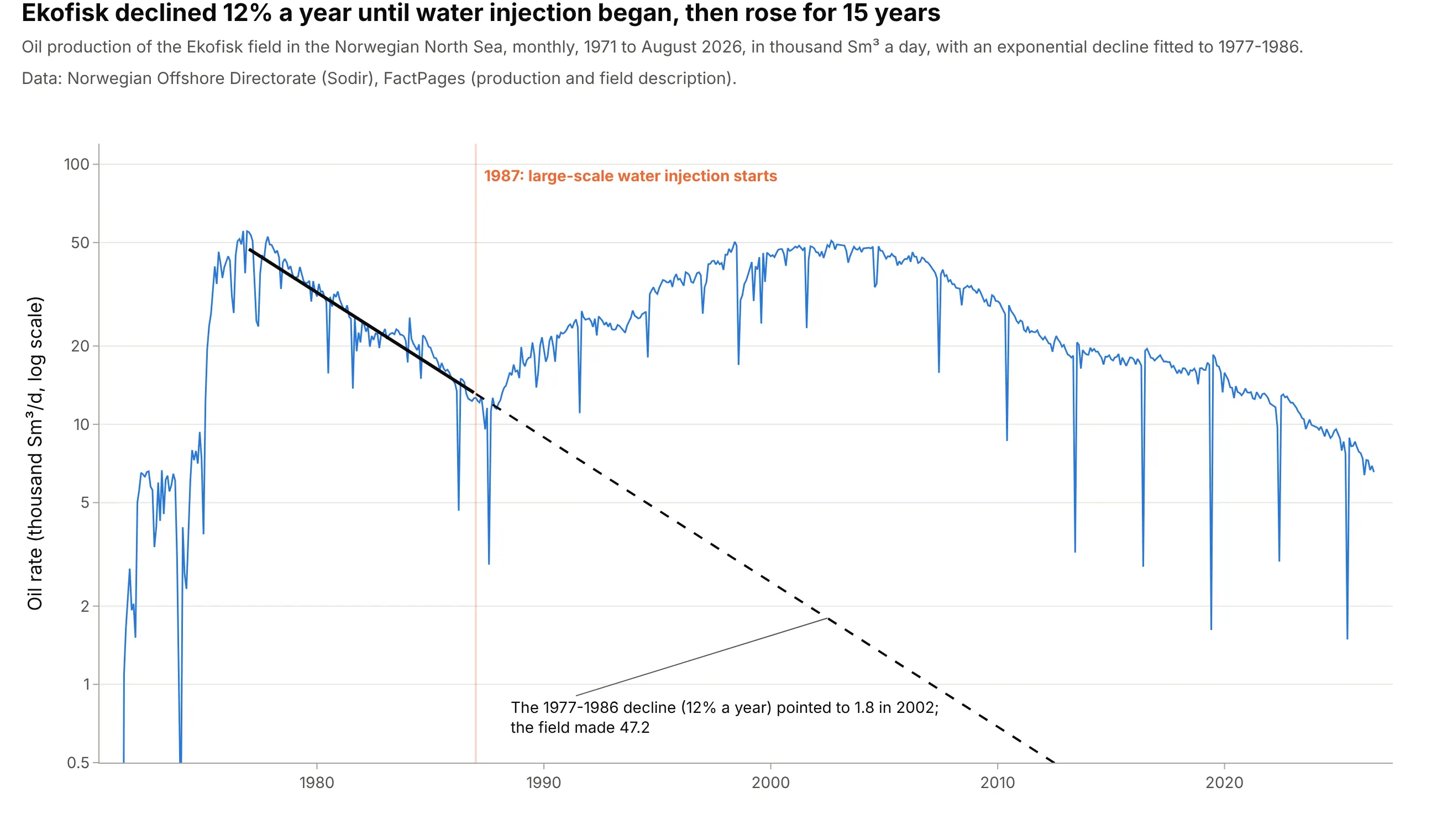
Ekofisk field oil rate on a log axis, 1971 to 2026: a black exponential fitted to 1977-1986 falls 12% a year, its dashed extension points to 1.8 thousand Sm³ a day in 2002, but after an orange line marking the start of large-scale water injection in 1987 the rate rises to about 47 in 2002

Ekofisk declined 12% a year from 1977 to 1986, and that decline pointed to 1.8 thousand Sm³ a day by 2002. Large-scale water injection started in 1987, and the field made 47.2 in 2002; Sodir says the expected recovery factor rose from 17% to over 50%. A decline curve assumes nothing about how the field is produced will change. Data: Sodir FactPages, field production and field description.

Tip: mark operational changes with a vertical line and never fit one curve across them.

Get the data from the Norwegian Offshore Directorate's FactPages (factpages.sodir.no, table field_production_monthly)
for EKOFISK and shape it into a monthly table (columns: date, oil_ksm3d).

Build a plotly line chart on a log y axis with an exponential fitted to 1977-1986 (solid) and extended to 2026
(dashed), and a vertical line at 1987 labeled with the start of large-scale water injection.