Chris Parmer

November 7, 2026

Bode Plots - A Complete Guide

TL;DR

A Bode plot shows how a system responds to sine waves of different frequencies in two stacked panels with a shared logarithmic frequency axis: the magnitude (gain) in decibels (dB) on top and the phase shift in degrees below.
Bode plots are also known as Bode diagrams, and the two panels as the Bode magnitude (or gain) plot and the Bode phase plot. They are one kind of frequency response plot, and are similar to line charts with two log-scaled axes, the Nyquist plot, and the Smith chart, which draw the same response in the complex plane.
Electrical and control engineers read four things off them: the cutoff frequency where the gain is down 3 dB, the roll-off slope (20 dB per decade for each pole), resonance peaks, and the gain and phase margins that say how far a feedback loop is from oscillating.
You can make a Bode plot with Plotly from two go.Scatter traces in make_subplots(rows=2, shared_xaxes=True) with a log x axis; scipy.signal computes the response from a transfer function. The code is below.

What is a Bode plot?

Bode plots look like this:

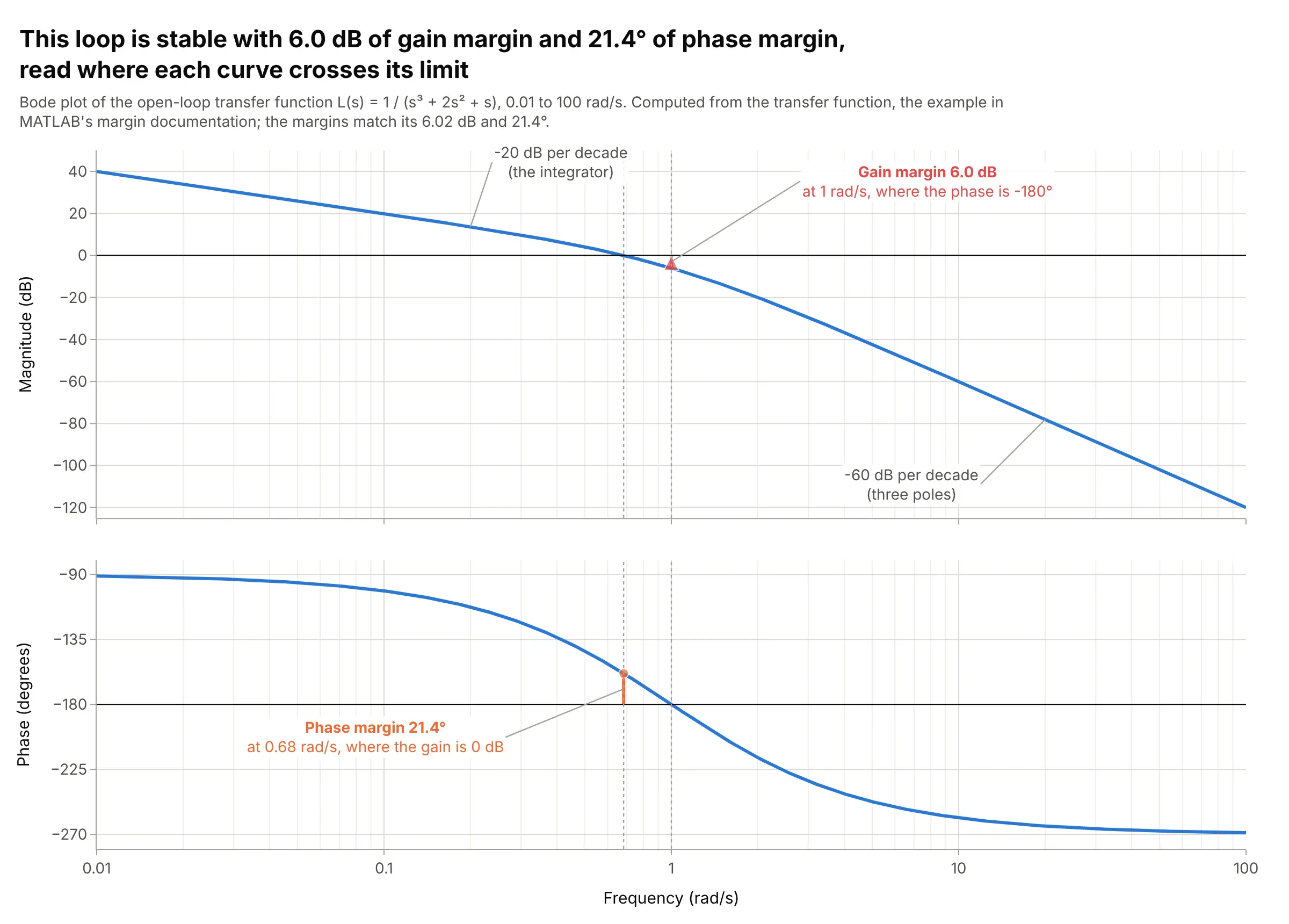
Bode plot of the loop L(s) = 1 / (s³ + 2s² + s) from 0.01 to 100 rad/s: the magnitude falls at -20 dB per decade, crosses 0 dB at 0.68 rad/s and then falls at -60 dB per decade; the phase falls from -90 to -270 degrees and crosses -180 at 1 rad/s, where the magnitude is 6.0 dB below 0 dB (the gain margin); at 0.68 rad/s the phase is 21.4 degrees above -180 (the phase margin)

Data: computed from the transfer function L(s) = 1 / (s³ + 2s² + s), the example in MATLAB’s margin documentation.

How do you read a Bode plot? In the example above, notice these things:

Each point is one frequency of a sine wave going around a feedback loop. The top panel says how much the loop amplifies it, in decibels, and the bottom panel how far the output sine lags behind the input, in degrees.
The frequency axis is logarithmic, so each gridline step (0.01, 0.1, 1, 10, 100 rad/s) is a factor of 10, called a decade. The magnitude falls 20 dB per decade at low frequencies and 60 dB per decade at high ones, because each of the loop’s three poles adds 20 dB per decade to the slope.
A loop with negative feedback oscillates if its gain is 0 dB (a factor of 1) when its phase is -180 degrees. Here the phase reaches -180 degrees at 1 rad/s, where the gain is -6.0 dB: the gain margin is 6.0 dB, so the gain could double before the loop oscillates.
The gain crosses 0 dB at 0.68 rad/s, where the phase is -158.6 degrees, 21.4 degrees short of -180: that’s the phase margin. MATLAB’s documentation reports the same 6.02 dB and 21.4 degrees for this loop, and 21 degrees is a small margin, which shows up as 54% overshoot in its step response (see the alternatives below).

It’s often used for charts like these:

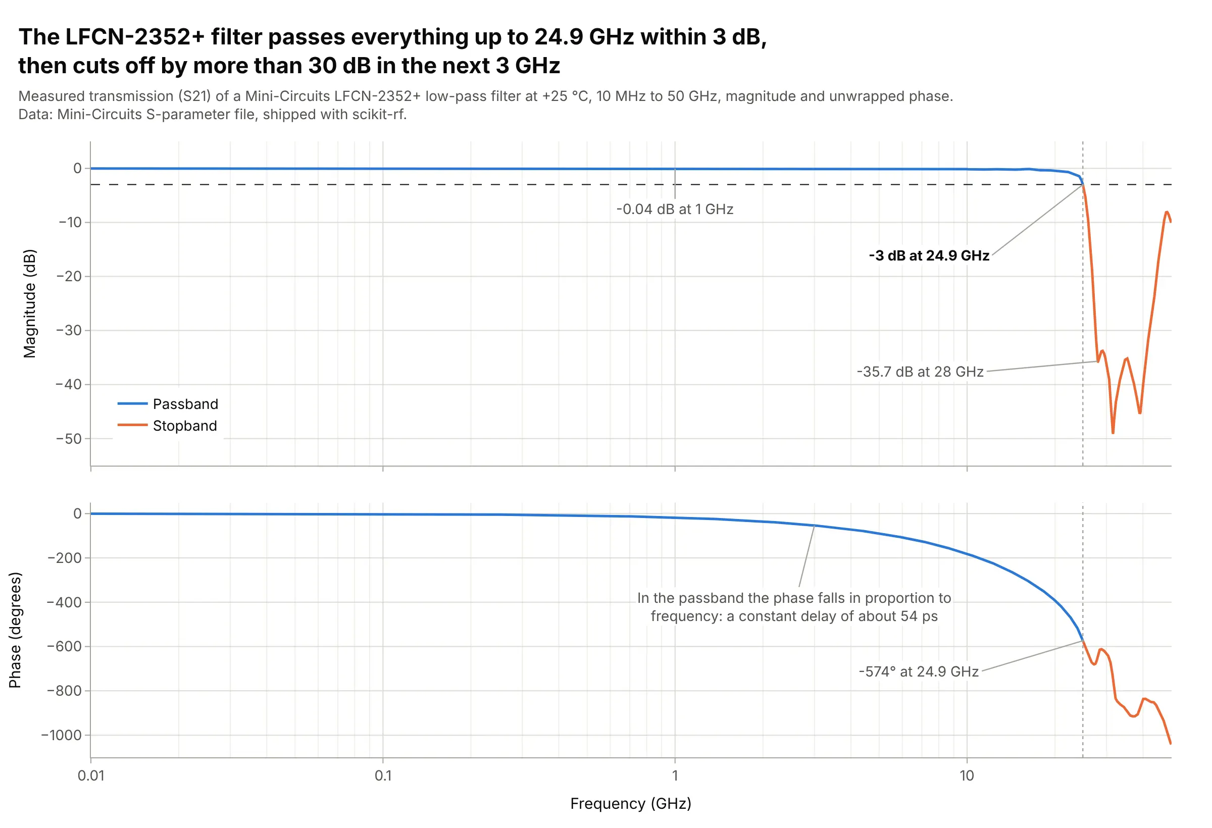
Bode plot of the measured transmission of a Mini-Circuits LFCN-2352+ low-pass filter from 10 MHz to 50 GHz: the magnitude stays near 0 dB up to the -3 dB point at 24.9 GHz, then plunges to about -35 dB by 28 GHz; the unwrapped phase falls steadily to -574 degrees at the cutoff

Filters. The LFCN-2352+ low-pass filter passes signals within 3 dB up to 24.9 GHz and is 35.7 dB down at 28 GHz, which a log frequency axis shows next to its flat passband from 10 MHz. Data: Mini-Circuits S-parameter file, shipped with scikit-rf (BSD-3-Clause).

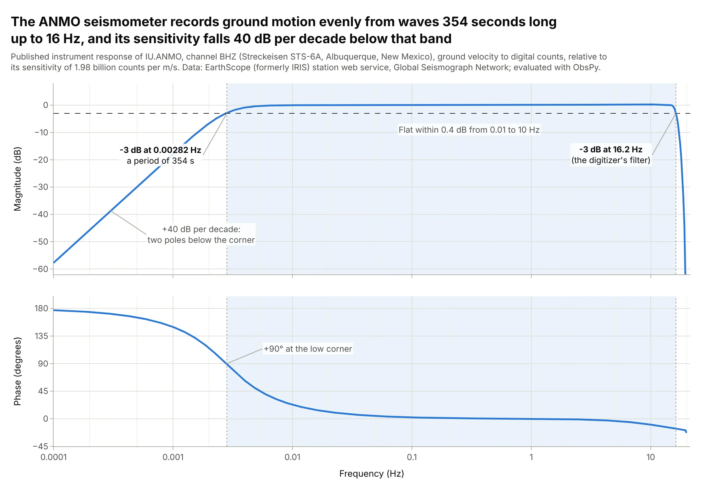
Bode plot of the published response of the IU.ANMO seismometer from 0.0001 to 20 Hz: the magnitude rises 40 dB per decade up to the -3 dB corner at 0.00282 Hz, stays flat to 16.2 Hz, and then drops steeply; the phase falls from +177 to 0 degrees, passing +90 degrees at the low corner

Sensors and instruments. The Streckeisen STS-6A seismometer at Albuquerque records ground motion within 3 dB from waves 354 seconds long up to 16.2 Hz, the band seismologists can trust when they correct records for the instrument. Data: EarthScope (formerly IRIS, the Incorporated Research Institutions for Seismology) station web service, Global Seismograph Network (GSN).

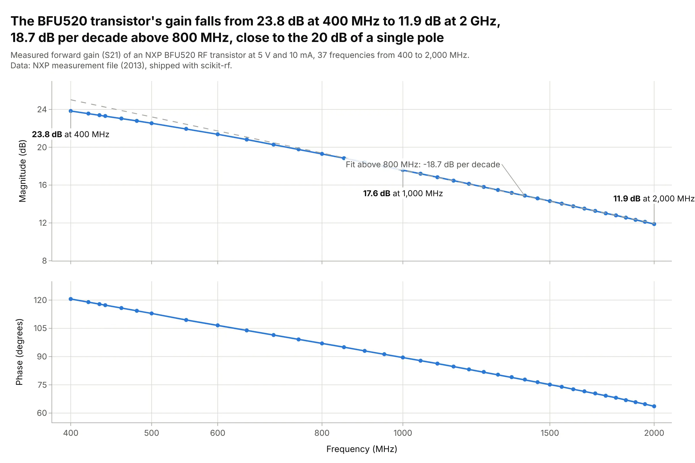
Bode plot of the measured forward gain of an NXP BFU520 transistor from 400 to 2,000 MHz: 37 points fall along a nearly straight line from 23.8 dB to 11.9 dB, with a dashed fit of -18.7 dB per decade above 800 MHz, and the phase falls from 121 to 64 degrees

Amplifiers. The gain of an NXP BFU520 radio-frequency (RF) transistor falls from 23.8 dB at 400 MHz to 11.9 dB at 2 GHz, 18.7 dB per decade, close to the 20 dB per decade of a single pole. Data: NXP measurement file, shipped with scikit-rf.

How to read a Bode plot

A Bode plot assumes two ideas that are second nature to electrical engineers and unusual everywhere else: decibels on the vertical axis and decades on the horizontal one. Once those are clear, cutoffs, slopes, resonances, and margins can be read straight off the chart.

Decibels

A decibel is a logarithmic way to write a ratio. For an amplitude ratio (a voltage, a current, a displacement), dB = 20 × log10(output / input), so a gain of 10 is +20 dB, a gain of 100 is +40 dB, and a gain of 0.1 is -20 dB:

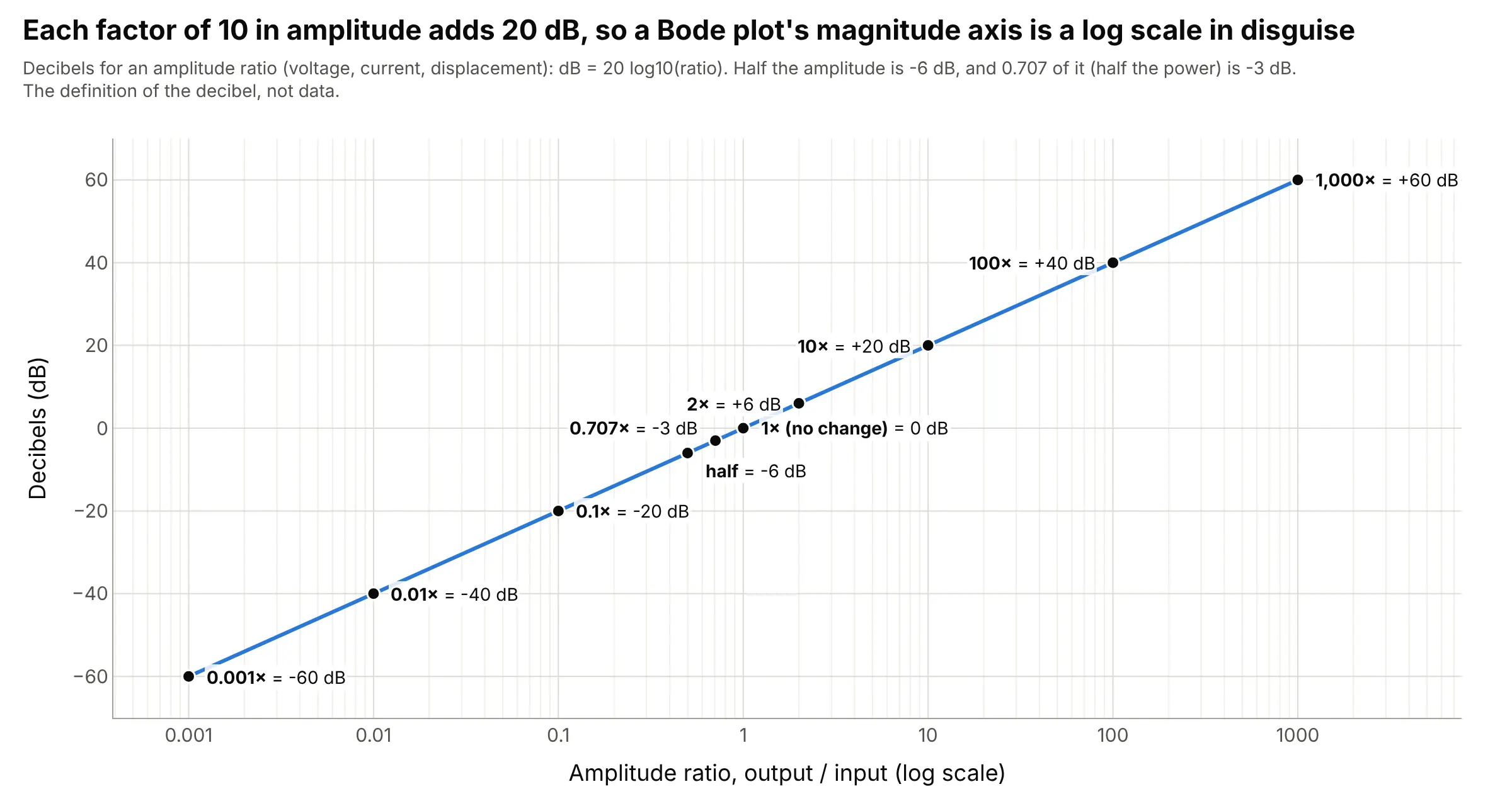
Data: the definition of the decibel (not data).

Decibels add where ratios multiply, which is why Bode chose them: the gain of two stages in a row is the sum of their curves. Half the amplitude is -6 dB, and 0.707 of it (1 / √2) is -3 dB, which is half the power, because power goes with the square of amplitude. For a power ratio, use 10 × log10 instead of 20 × log10.

Decades and the log frequency axis

The frequency axis is logarithmic, so each factor of 10 in frequency, called a decade, gets the same width. A factor of two is an octave, and one decade is about 3.3 octaves. This lets one chart show 10 Hz and 100 kHz together, and it turns the power laws of circuits and mechanisms into straight lines, since a gain proportional to 1/f falls the same 20 dB in every decade.

Cutoff frequency (-3 dB)

The cutoff (or corner) frequency is where the gain has fallen 3 dB below its flat value, and half the power gets through. For a first-order resistor-capacitor (RC) low-pass filter, it is also where the phase lag is exactly 45 degrees:

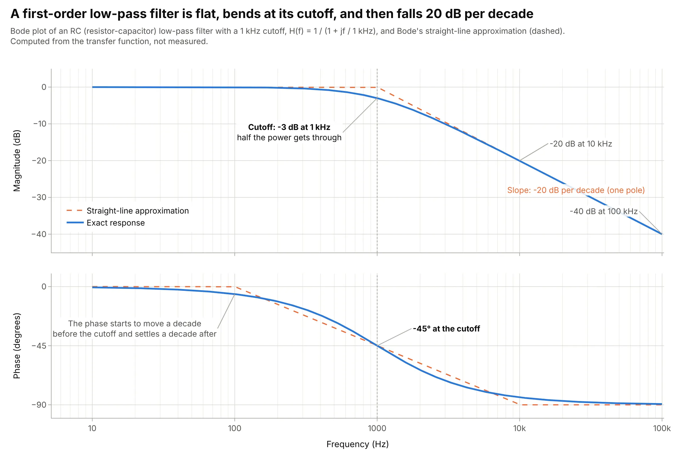
Bode plot of an RC low-pass filter with a 1 kHz cutoff: the magnitude is flat, is -3 dB at 1 kHz, and falls 20 dB per decade to -40 dB at 100 kHz, with an orange dashed straight-line approximation; the phase falls from 0 to -90 degrees, passing -45 at 1 kHz

Data: computed from H(f) = 1 / (1 + jf / 1 kHz), not measured.

The dashed lines are Bode’s straight-line (asymptotic) approximation: flat up to the cutoff, then a straight slope. The real curve is 3 dB below the corner of the straight lines, and the phase moves from about one decade before the cutoff to one decade after (from -5.7 degrees at 100 Hz to -84.3 degrees at 10 kHz).

Roll-off: 20 dB per decade per pole

Above its cutoff, each pole (each independent energy store, like a capacitor or a mass) makes the gain fall another 20 dB per decade (6 dB per octave) and adds up to 90 degrees of phase lag. Each zero does the opposite:

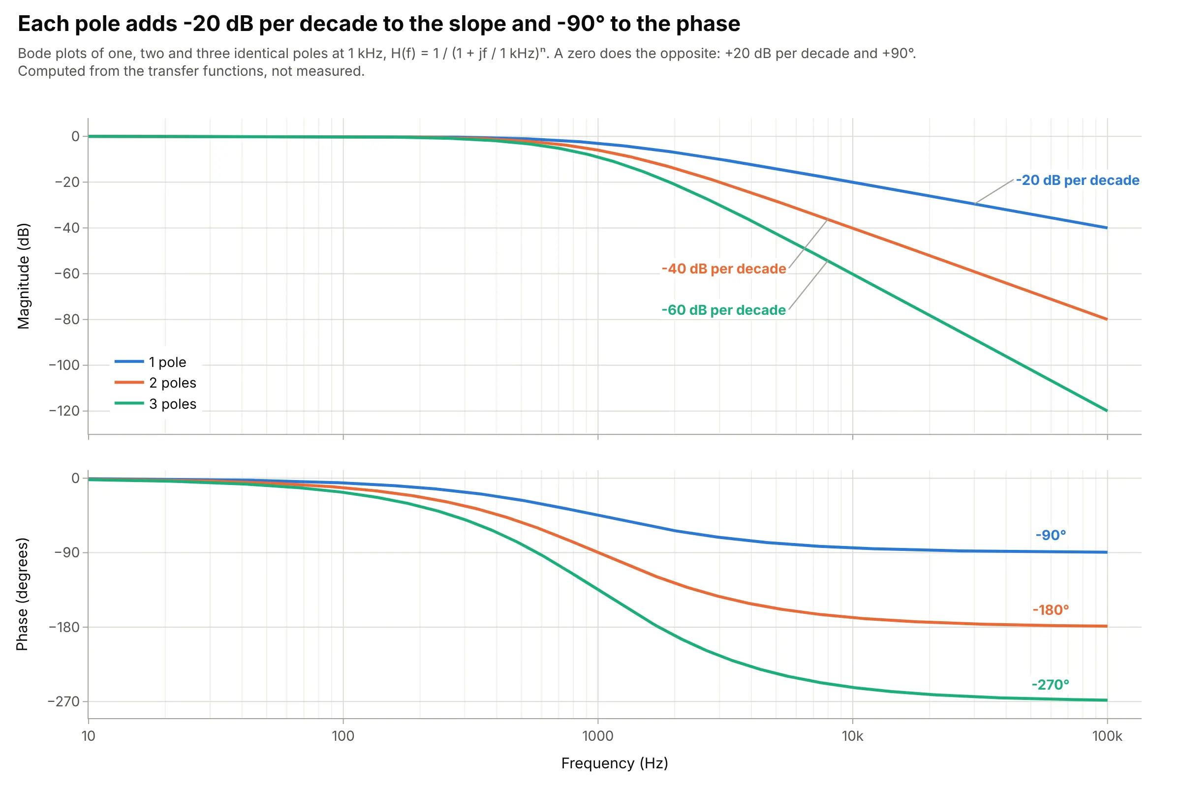
Bode plots of one, two, and three poles at 1 kHz: the magnitudes fall at -20, -40, and -60 dB per decade, and the phases settle at -90, -180, and -270 degrees

Data: computed from H(f) = 1 / (1 + jf / 1 kHz)ⁿ, not measured.

That’s why you can count the poles of a system from the slope of its measured response, and why the main example above, with three poles, ends at -60 dB per decade and -270 degrees.

Resonance peaks

A pair of poles with little damping makes a resonance: a peak in the magnitude and a fast 180-degree swing in the phase at the natural frequency. The damping ratio ζ (zeta) sets how tall the peak is:

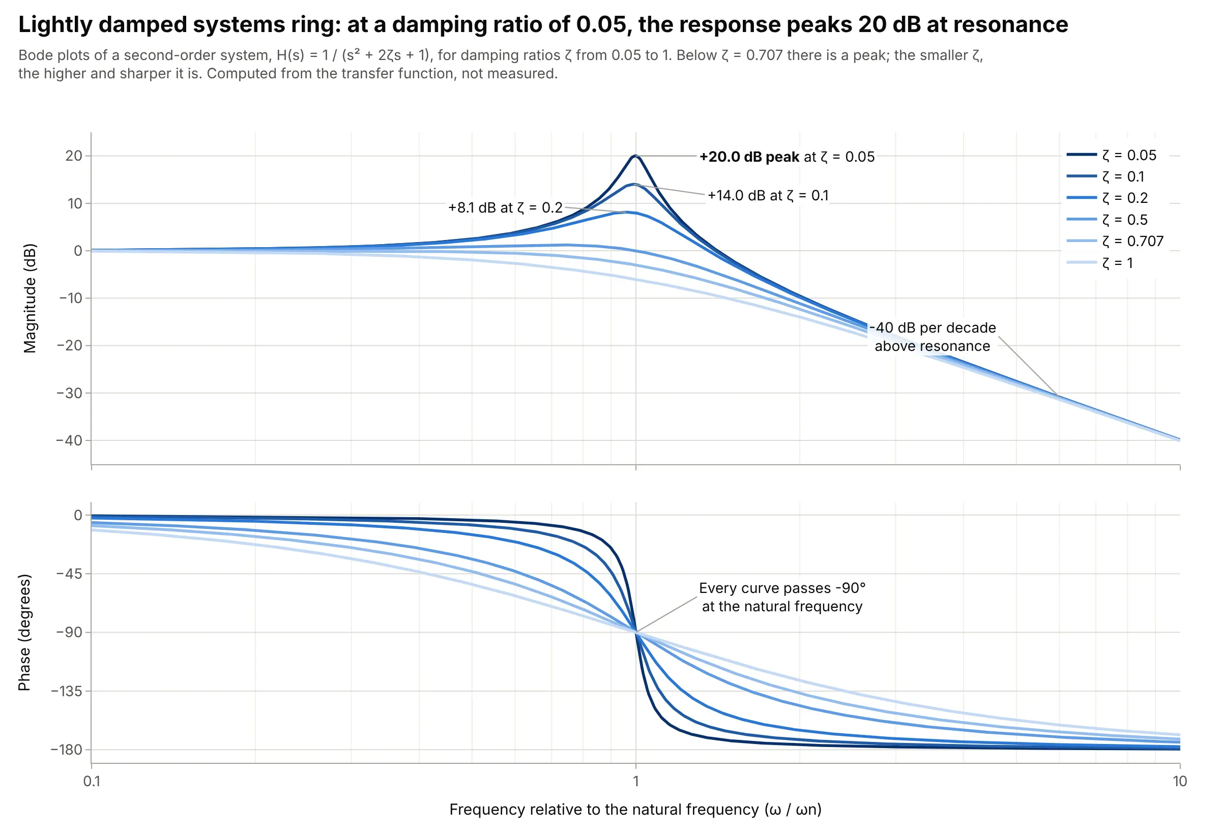
Bode plots of a second-order system for damping ratios from 0.05 to 1: the magnitude peaks at +20.0 dB for zeta 0.05, +14.0 dB for 0.1, and +8.1 dB for 0.2 near the natural frequency and has no peak for 0.707 and 1; every phase curve passes -90 degrees at the natural frequency

Data: computed from H(s) = 1 / (s² + 2ζs + 1), not measured.

At ζ = 0.05 the peak is +20.0 dB, a factor of 10, so a sine at that frequency comes out 10 times larger than it went in. Above ζ = 0.707 there is no peak. Resonances in measured data, like the robot arm under More examples, show up the same way.

Gain and phase margins

For a feedback loop, plot the open-loop response (everything around the loop, with the loop cut open) and find two frequencies, as in the main example. At the phase crossover, where the phase is -180 degrees, the gain margin is how far the gain is below 0 dB. At the gain crossover, where the gain is 0 dB, the phase margin is how far the phase is above -180 degrees. A loop is stable with margin to spare when both are positive, and common targets are at least 6 dB of gain margin and 45 to 60 degrees of phase margin (Wikipedia cites 45 degrees as a rule of thumb for good step response).

Bode plots, Nyquist plots, and Smith charts

A Nyquist plot draws the same open-loop response as one curve in the complex plane (real part against imaginary part), and Harry Nyquist’s 1932 criterion reads stability from how it circles the point -1 (Nyquist 1932). It handles loops where the margins are ambiguous, but it hides frequency along the curve. RF engineers draw reflection measurements on a Smith chart, which is a polar plot of the reflection coefficient with impedance circles on top, and use Bode-style plots of |S21| in dB against frequency for gain and filtering. The alternatives figure below shows a Nyquist plot of the main example.

A short history

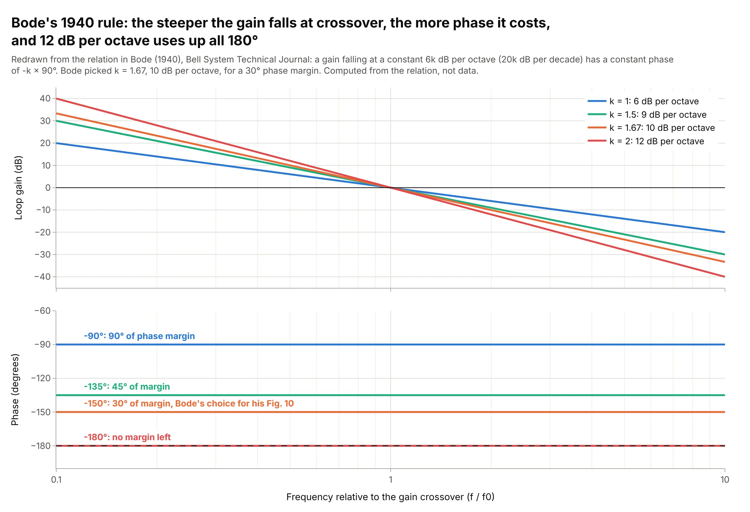
Hendrik Bode, an engineer at Bell Telephone Laboratories, developed the plots in the 1930s while designing stable feedback amplifiers for telephone networks (Wikipedia), and published the theory in “Relations Between Attenuation and Phase in Feedback Amplifier Design” in the Bell System Technical Journal in July 1940 (Bode 1940; scan on archive.org). Its central result is that, for most circuits, the phase follows from the slope of the gain, and the paper defined the phase and gain margins (“Diagram to illustrate definitions of phase and gain margins for the feedback loop”, its Fig. 9). This is its constant-slope rule, redrawn:

Four loop gains falling at constant slopes of 6, 9, 10, and 12 dB per octave through 0 dB, and their constant phases of -90, -135, -150, and -180 degrees, labeled with 90, 45, 30, and 0 degrees of phase margin

Data: computed from the relation in H. W. Bode, “Relations Between Attenuation and Phase in Feedback Amplifier Design”, Bell System Technical Journal 19(3), 421-454, 1940.

Bode wrote that a gain with “a constant slope of 6k db per octave” has a constant phase of kπ/2 radians, k × 90 degrees. At 12 dB per octave the phase is 180 degrees and the loop has no margin, so he chose k = 1.67, a cutoff of 10 dB per octave with a 30-degree phase margin, for his ideal loop in Fig. 10.

Alternatives to a Bode plot

Here’s the same feedback loop drawn six ways. Some are better for the question, some worse, some just different:

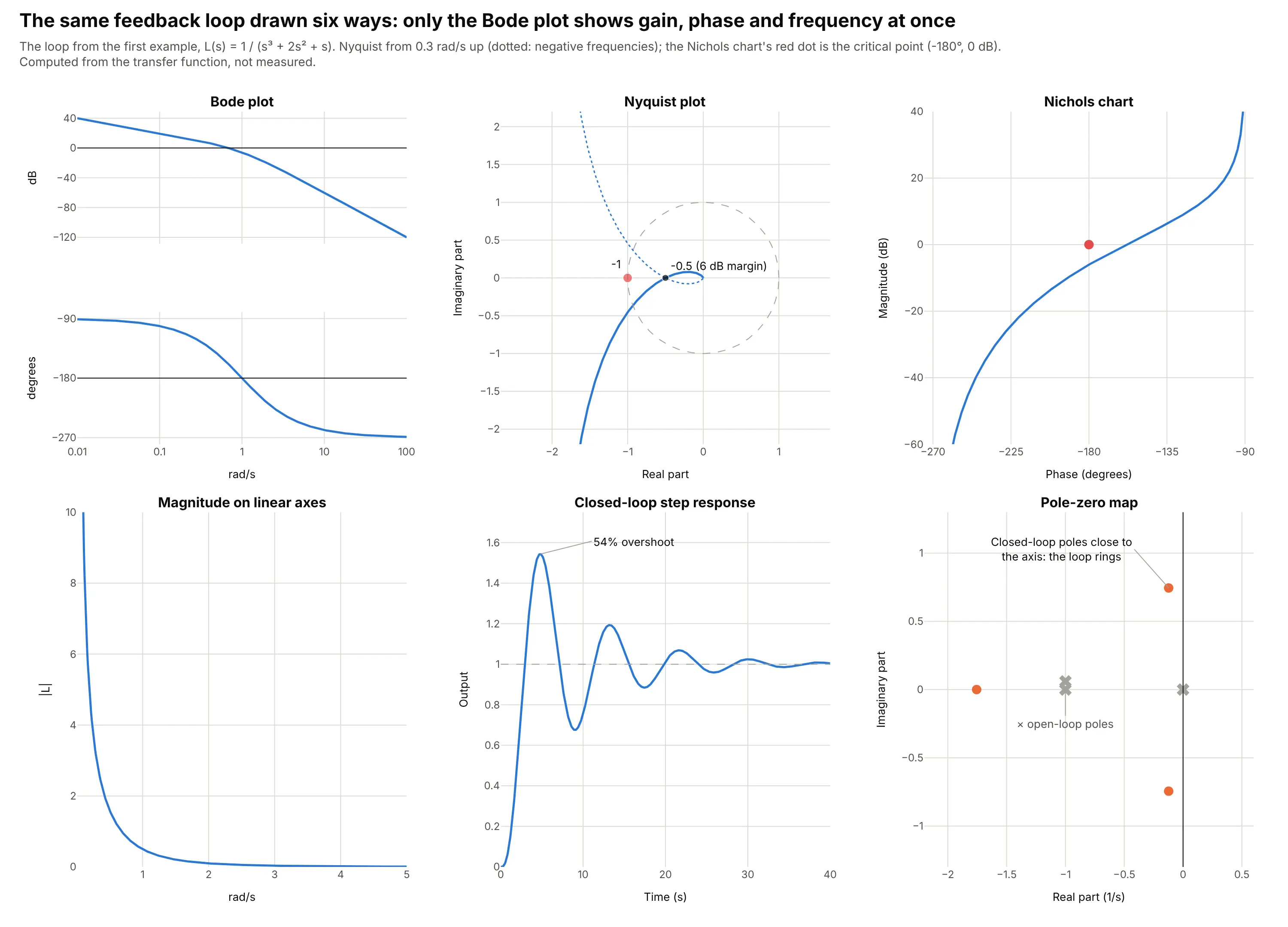
Six charts of the loop L(s) = 1 / (s³ + 2s² + s): a Bode plot with magnitude and phase panels, a Nyquist plot whose curve crosses the negative real axis at -0.5 inside the unit circle, a Nichols chart of magnitude against phase passing below the critical point at -180 degrees and 0 dB, the magnitude on linear axes falling from 10 to near zero by 1 rad/s, a closed-loop step response with 54% overshoot and slow ringing, and a pole-zero map with two closed-loop poles close to the imaginary axis

Nyquist plot (works too, for stability). It shows the margins as distances from the point -1: the curve crosses the negative real axis at -0.5, which is the 6 dB gain margin. It’s the safer test for loops with several crossovers, but frequency is hidden along the curve.
Nichols chart (works too, for loop shaping). Magnitude in dB against phase in degrees puts the critical point at (-180 degrees, 0 dB), and control engineers overlay closed-loop contours on it. Frequency is again only a label on the curve.
Magnitude on linear axes (worse). Everything above 1 rad/s collapses onto zero and the phase is gone, so neither margin can be read.
Step response (different). It shows what users feel, 54% overshoot and ringing still visible after 30 seconds, but not why, or which frequency to fix.
Pole-zero map (different). Two closed-loop poles close to the imaginary axis explain the ringing, but a measured system rarely comes with poles, while a frequency response can always be measured.

A dual-axis chart with magnitude and phase on one panel saves space but makes readers match each curve to its axis, so two stacked panels with a shared x axis are the convention. When you compare many systems, small multiples of Bode plots work better than one crowded pair of panels.

How to make a Bode plot

With AI

ChatGPT, Claude Code, GitHub Copilot, Cursor, and other AI tools are excellent at writing Plotly code. Name Plotly in the prompt, and say whether the response comes from a transfer function or from measured data, and which units you want:

Make a plotly Bode plot of the open-loop transfer function L(s) = 1 / (s^3 + 2s^2 + s).

- Compute magnitude (dB) and phase (degrees, unwrapped) with scipy.signal.bode from 0.01 to 100 rad/s.
- Use make_subplots(rows=2, shared_xaxes=True), magnitude on top, phase below, x axis type "log".
- Add reference lines at 0 dB and -180 degrees, mark the gain and phase crossover frequencies,
  and annotate the gain margin and phase margin.
- Check: print the margins and compare them with control.margin or MATLAB (6.02 dB, 21.4 degrees).

With Plotly Studio

Plotly Studio is a desktop app where you point an AI at a dataset and it builds charts and a Dash app around your questions. Ask for a Bode plot the same way:

Show a Bode plot of S21 from this Touchstone file: magnitude in dB on top, unwrapped phase in degrees below, a shared log frequency axis in GHz, a dashed line at -3 dB with the cutoff frequency labeled, and a dropdown to pick the temperature.

Make a Bode plot in Python or JavaScript

This is the code AI tools write under the hood. Plotly has no dedicated Bode trace, so a Bode plot is two go.Scatter traces in make_subplots(rows=2, shared_xaxes=True) with a log x axis. This helper returns a go.Figure, and every example in this guide builds on the same idea:

import numpy as np
import plotly.graph_objects as go
from plotly.subplots import make_subplots
from scipy import signal


def bode_plot(freq, mag_db, phase_deg, name=None, color="#2a78d6"):
    """A Bode plot in Plotly: magnitude on top, phase below, one shared log frequency axis."""
    fig = make_subplots(rows=2, cols=1, shared_xaxes=True, vertical_spacing=0.06)
    fig.add_trace(go.Scatter(x=freq, y=mag_db, name=name, line_color=color), row=1, col=1)
    fig.add_trace(go.Scatter(x=freq, y=phase_deg, name=name, line_color=color, showlegend=False), row=2, col=1)
    fig.update_xaxes(type="log")
    fig.update_xaxes(title_text="Frequency (rad/s)", row=2, col=1)
    fig.update_yaxes(title_text="Magnitude (dB)", row=1, col=1)
    fig.update_yaxes(title_text="Phase (degrees)", row=2, col=1)
    fig.update_layout(template="simple_white", hovermode="x unified", showlegend=name is not None)
    return fig


# The feedback loop from the first example: L(s) = 1 / (s^3 + 2s^2 + s)
loop = signal.TransferFunction([1], [1, 2, 1, 0])
w, mag, phase = signal.bode(loop, w=np.logspace(-2, 2, 500))  # rad/s, dB, degrees

fig = bode_plot(w, mag, phase)
fig.add_hline(y=0, line_width=1, line_dash="dot", line_color="gray", row=1, col=1)     # gain crossover reference
fig.add_hline(y=-180, line_width=1, line_dash="dot", line_color="gray", row=2, col=1)  # phase crossover reference
fig.show()

For measured data, such as a Touchstone file from a vector network analyzer (VNA), read it with scikit-rf and pass 20 * np.log10(np.abs(s21)) and np.degrees(np.unwrap(np.angle(s21))). For a system you can only record in time, estimate the response from the input and output with scipy.signal.csd divided by scipy.signal.welch, or with the ratio of their Fourier transforms at the excited frequencies, as the robot arm example does.

In JavaScript, plotly.js draws the same thing with two traces on one shared x axis and two y axes:

<div id="chart"></div>
<script src="https://cdn.plot.ly/plotly-4.1.1.min.js"></script>
<script>
  // The feedback loop from the first example, L(s) = 1 / (s (s + 1)^2), at 400 frequencies from 0.01 to 100 rad/s
  const w = Array.from({length: 400}, (_, i) => 10 ** (-2 + 4 * i / 399));
  const mag = w.map(x => -20 * Math.log10(x * (1 + x * x)));            // |L| in dB
  const phase = w.map(x => -90 - 2 * Math.atan(x) * 180 / Math.PI);     // angle of L in degrees

  const line = {color: "#2a78d6", width: 2.5};
  const ref = (y, yref) => ({type: "line", xref: "paper", x0: 0, x1: 1, yref: yref, y0: y, y1: y,
                             line: {color: "gray", dash: "dot", width: 1}});
  Plotly.newPlot("chart", [
    {x: w, y: mag, mode: "lines", line: line, xaxis: "x", yaxis: "y"},
    {x: w, y: phase, mode: "lines", line: line, xaxis: "x", yaxis: "y2"}
  ], {
    width: 900, height: 600, showlegend: false, hovermode: "x unified",
    grid: {rows: 2, columns: 1},
    xaxis: {type: "log", title: {text: "Frequency (rad/s)"}},
    yaxis: {domain: [0.55, 1], title: {text: "Magnitude (dB)"}},
    yaxis2: {domain: [0, 0.45], title: {text: "Phase (degrees)"}, dtick: 45},
    shapes: [ref(0, "y"), ref(-180, "y2")]
  });
</script>

Share it

Every Plotly chart has a Share chart button (the cloud icon in its toolbar) that uploads it to Plotly Cloud and gives you a link. Only you can see it until you change its visibility.

For a live app, put the chart in a Dash app and publish it with the Plotly Cloud CLI. Coding agents can run these commands for you:

pip install "dash[cloud]"
plotly user login
plotly app publish

If your data has to stay in your own cloud or data center, publish to Dash Enterprise instead.

Dos and don’ts

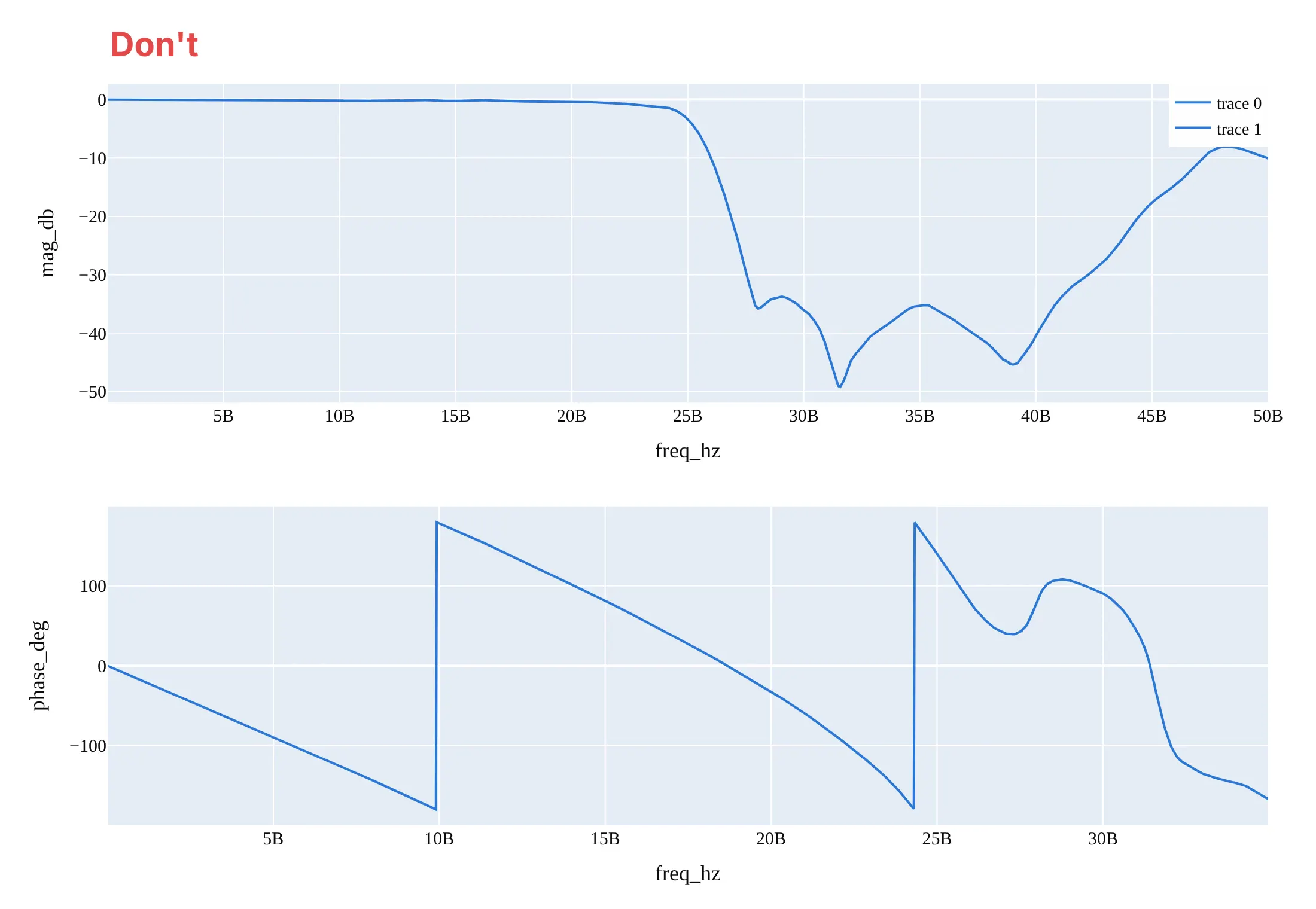
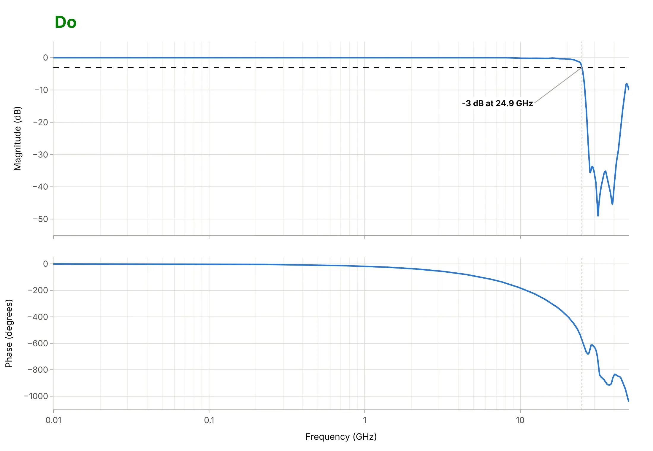
Most Bode plots that are hard to read break the conventions engineers expect: a log frequency axis, dB, unwrapped phase, and two aligned panels. Here is the measured LFCN-2352+ filter both ways, in the same blue.

Don’t plot frequency on a linear axis (the 10 MHz to 1 GHz range, two of the three decades of passband, is squeezed against the left edge), leave the phase wrapped so it jumps from -180 to +180 degrees, give the two panels different x ranges, label the axes with raw column names and “5B” for 5 billion hertz, and keep a serif font and a legend of “trace 0” and “trace 1”:

The filter’s magnitude and wrapped phase against a linear frequency axis labeled freq_hz with ticks 5B to 50B, the phase panel’s axis ending at 35B so the panels don’t line up, sawtooth jumps in the phase at 10 and 24 GHz, a legend reading trace 0 and trace 1, a serif font, and a blue-gray background

Do share one log frequency axis in GHz between the panels, unwrap the phase, give each axis a name and a unit, and mark the -3 dB line and the cutoff frequency in both panels:

The same filter on a shared log axis from 0.01 to 50 GHz in two panels, magnitude in dB with a dashed -3 dB line and a label at 24.9 GHz, unwrapped phase falling smoothly to -1,000 degrees, and a dotted line at the cutoff through both panels

Checklist

Use a log frequency axis and say whether it is in Hz or rad/s (1 Hz is 2π rad/s).
Stack magnitude above phase with one shared x axis, so a frequency lines up in both panels.
Draw the reference lines readers look for: -3 dB for filters, 0 dB and -180 degrees for feedback loops.
Unwrap the phase, or say on the chart that it is wrapped to ±180 degrees.
Label what was measured and what was computed, and the reference for 0 dB (1 kHz, the sensitivity, the input).

Don’t

Put magnitude and phase on one panel with two y axes.
Mix 10 log10 (power) and 20 log10 (amplitude) decibels on one chart.
Trust the phase or the margins of a measurement where the signal is buried in noise, such as a filter’s deep stopband.
Draw a closed-loop response and read stability margins from it; margins come from the open loop.

Options to customize

A Bode plot in Plotly is two go.Scatter traces in subplots, so these are the options that matter most. The full lists are in the scatter trace reference, the subplots documentation, and the log axes documentation.

make_subplots(rows=2, cols=1, shared_xaxes=True): the two panels with one frequency axis, so zooming one zooms both.
row_heights=[0.55, 0.45] and vertical_spacing: give the magnitude a little more room and keep the panels close.
fig.update_xaxes(type="log"): the logarithmic frequency axis; dtick=1 puts a tick at every decade.
xaxis.minor.showgrid: faint gridlines at 2, 3, ... 9 within each decade, which make values easy to read off.
tickvals and ticktext: custom ticks like 20, 50, 100 ... 20k for audio, or 1/2/5 steps.
yaxis.dtick: 20 dB steps for magnitude and 45 or 90 degrees for phase.
fig.add_hline(y=-3, row=1, col=1) and fig.add_vline(x=fc): the -3 dB line, 0 dB and -180 degrees, and crossover or cutoff frequencies through both panels.
fig.add_annotation(x=np.log10(f), ...): labels on a log axis take the log of the frequency.
hovermode="x unified": one hover box with magnitude and phase at the same frequency.
go.Scattergl: WebGL traces for sweeps of hundreds of thousands of points.

More Bode plot examples

Seven more Bode plots, each with its source, the technique that makes it work, and a prompt to rebuild it. Four use measured data, and three are textbook cases computed from their definitions.

1. Four classic filters with the same order and cutoff

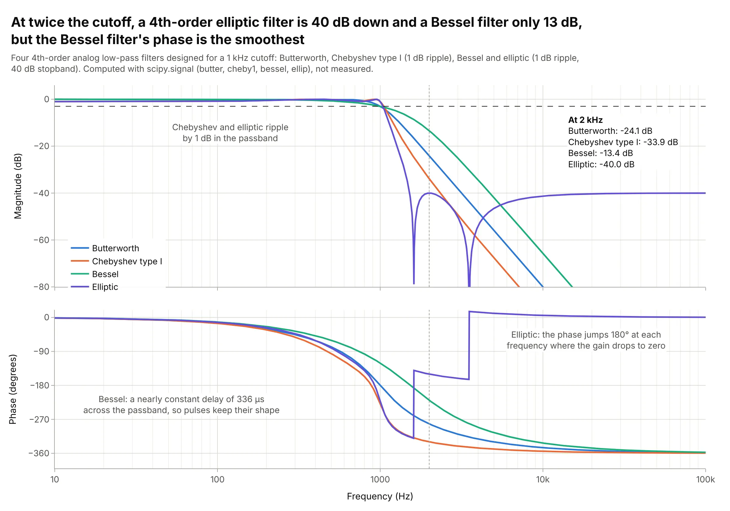
Bode plot of 4th-order Butterworth, Chebyshev type I, Bessel, and elliptic low-pass filters at 1 kHz: at 2 kHz they are down 24.1, 33.9, 13.4, and 40.0 dB, the elliptic filter has nulls and a 40 dB floor, and the Bessel phase is the smoothest

One octave above a 1 kHz cutoff, a 4th-order elliptic filter is down 40.0 dB and a Bessel filter only 13.4 dB, but the Bessel filter delays every frequency in its passband by nearly the same 336 µs, so pulses keep their shape. The Bode plot shows that trade-off in one view. Data: computed with scipy.signal (butter, cheby1, bessel, ellip), not measured.

Tip: mark one frequency just above the cutoff with a dotted line and list each curve’s value there.

Make a plotly Bode plot comparing four 4th-order analog low-pass filters with a 1 kHz cutoff, designed with
scipy.signal: butter, cheby1 (1 dB ripple), bessel (norm="mag") and ellip (1 dB ripple, 40 dB stopband).

Magnitude and unwrapped phase from 10 Hz to 100 kHz in two rows with a shared log x axis, a -3 dB line,
a dotted line at 2 kHz and each filter's attenuation there in a text box.

2. A flexible robot arm’s measured resonances

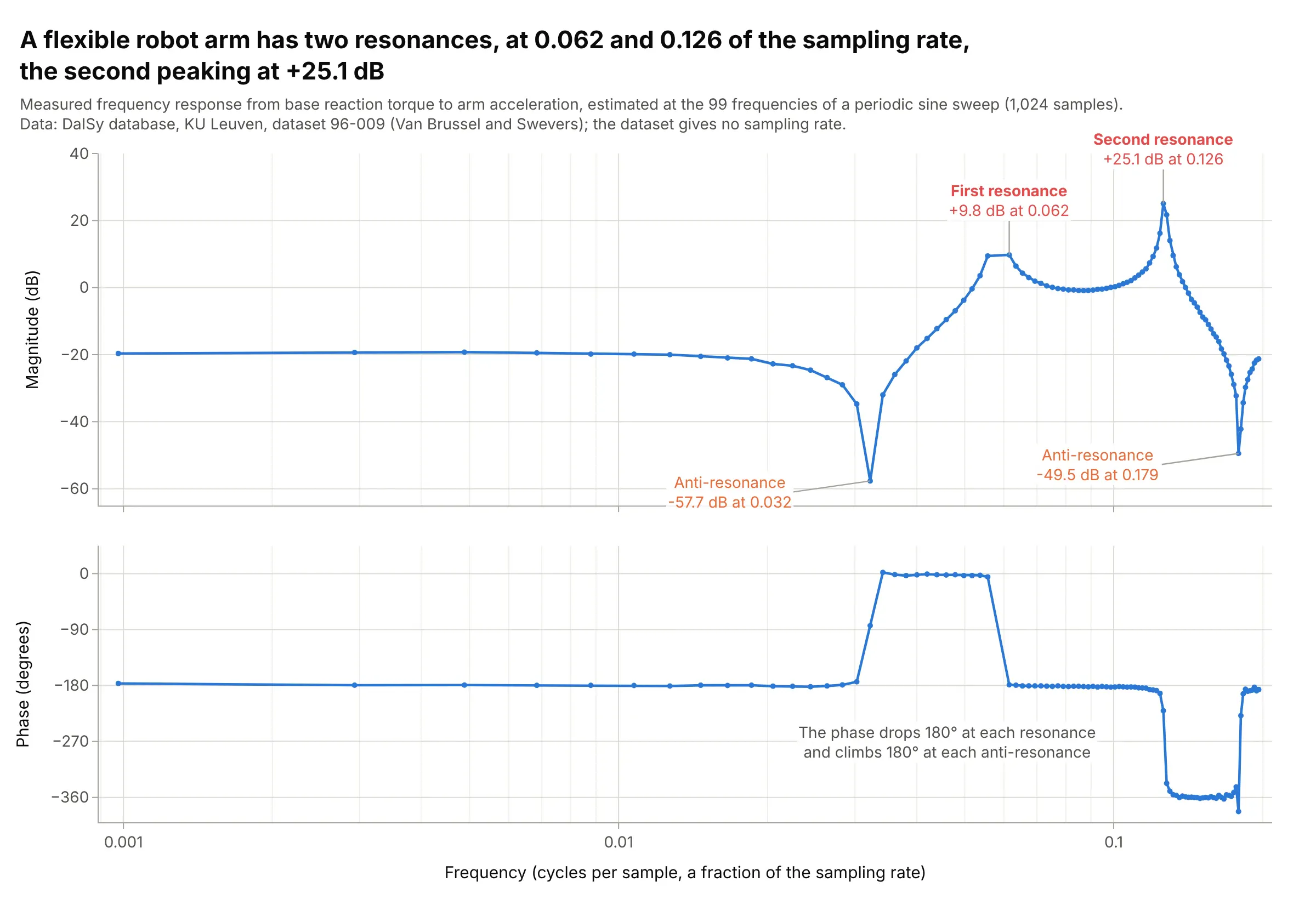
$Measured Bode plot of a flexible robot arm against frequency as a fraction of the sampling rate: the magnitude is about -20 dB at low frequency, dips to -57.7 dB at 0.032, peaks at +9.8 dB at 0.062 and +25.1 dB at 0.126, and dips again to -49.5 dB at 0.179; the phase steps up 180 degrees at each dip and down 180 at each peak$

The arm has two resonances, at 0.062 and 0.126 of the sampling rate, the second peaking at +25.1 dB, and an anti-resonance (a dip) before each. A controller for this arm must keep its gain low near those peaks, which is why mechanical engineers measure a frequency response before they tune a loop. Data: DaISy (Database for the Identification of Systems), KU Leuven, dataset 96-009; it gives no sampling rate.

Tip: draw the measured frequencies as markers on the line, so readers can see how densely each resonance was measured.

Get the data from the DaISy database at KU Leuven (homes.esat.kuleuven.be/~smc/daisy, dataset 96-009,
robot_arm.dat.gz: 1,024 samples of input u, reaction torque, and output y, arm acceleration, from a periodic sine
sweep) and estimate the frequency response as FFT(y) / FFT(u) at the excited bins (columns: freq_cycles_per_sample,
mag_db, phase_deg).

Make a plotly Bode plot with a shared log x axis, markers on the line, and the resonance peaks and dips labeled.

3. The RIAA curve every record player applies

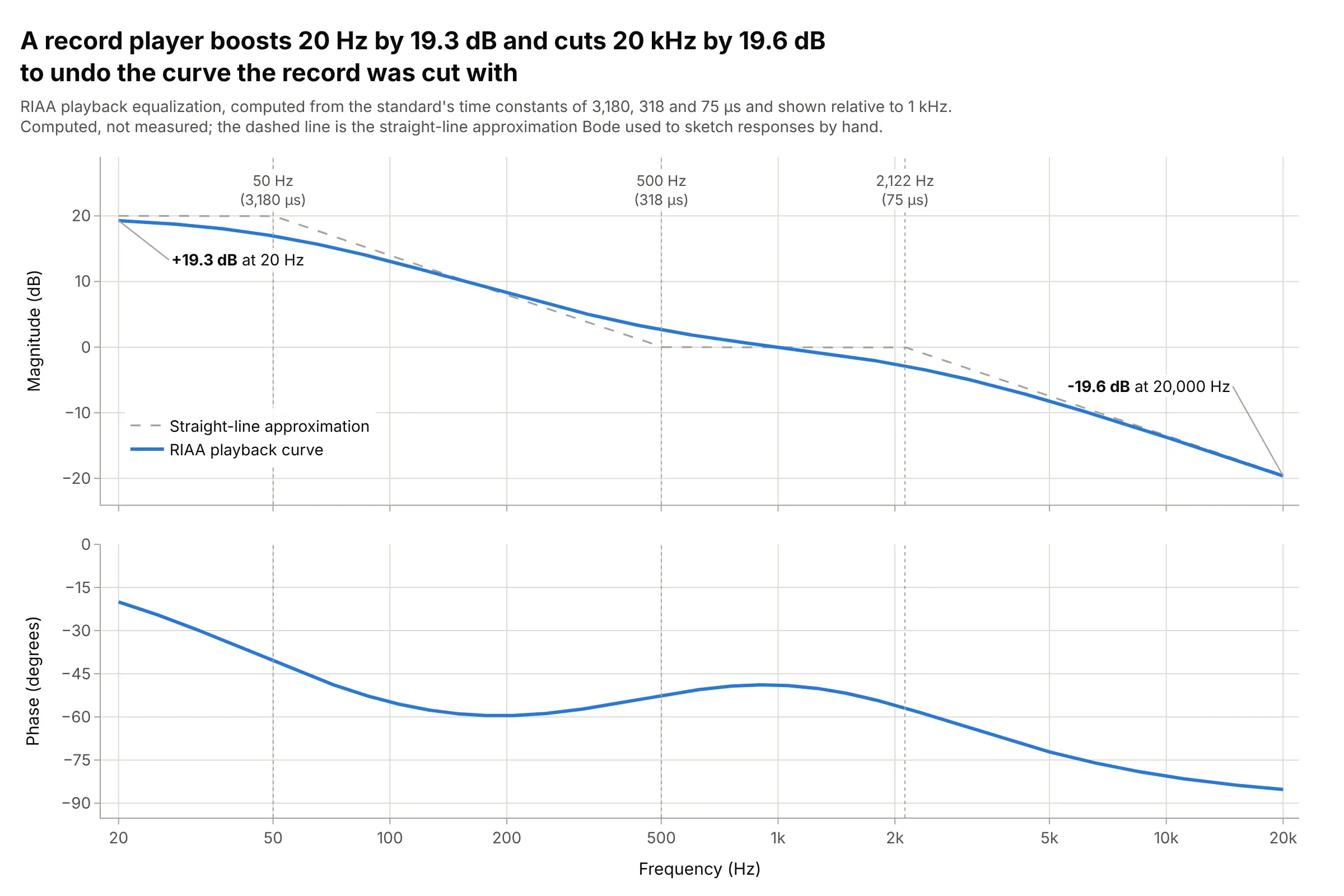
Bode plot of the RIAA playback curve from 20 Hz to 20 kHz relative to 1 kHz: the magnitude falls from +19.3 dB at 20 Hz to -19.6 dB at 20 kHz, with dotted corner lines at 50, 500, and 2,122 Hz and a dashed straight-line approximation; the phase dips to about -60 degrees near 200 Hz and falls to -85 degrees at 20 kHz

Records are cut with the bass turned down and the treble turned up, and every phono preamp undoes it with the curve set by the Recording Industry Association of America (RIAA): +19.3 dB at 20 Hz and -19.6 dB at 20 kHz relative to 1 kHz. Its three time constants put corners at 50, 500, and 2,122 Hz. Data: computed from the RIAA time constants of 3,180, 318, and 75 µs (Wikipedia), not measured.

Tip: draw the corner frequencies as dotted lines and label them with the time constants that set them.

Make a plotly Bode plot of the RIAA playback equalization curve, H(s) = (1 + s*318us) / ((1 + s*3180us)(1 + s*75us)),
normalized to 0 dB at 1 kHz, from 20 Hz to 20 kHz.

Two rows with a shared log x axis ticked 20, 50, 100 ... 20k, the straight-line approximation dashed, and dotted
lines at the three corner frequencies.

4. A lead compensator doubles the phase margin

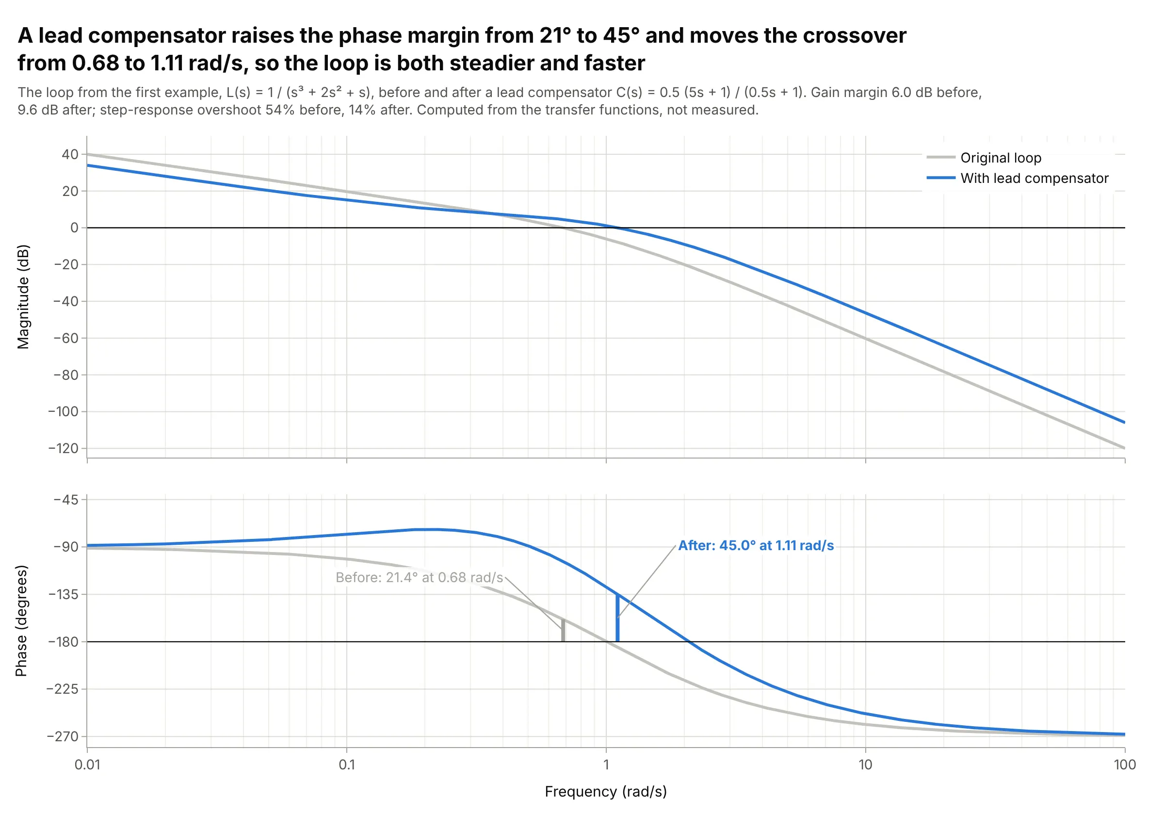
Bode plot of the loop from the first example before (gray) and after (blue) a lead compensator: the blue magnitude crosses 0 dB later, at 1.11 rad/s, and the blue phase bulges upward, leaving 45.0 degrees of phase margin against 21.4 before

A lead compensator, C(s) = 0.5 (5s + 1) / (0.5s + 1), adds phase near the crossover, raising the main example’s phase margin from 21 to 45 degrees and its gain margin from 6.0 to 9.6 dB, while the crossover moves from 0.68 to 1.11 rad/s. In the time domain, overshoot falls from 54% to 14%. Data: computed from the transfer functions, not measured.

Tip: draw the original loop in gray behind the new one, so the change is the only thing in color.

Make a plotly Bode plot of L(s) = 1 / (s^3 + 2s^2 + s) with and without a lead compensator
C(s) = 0.5 (5s + 1) / (0.5s + 1), from 0.01 to 100 rad/s.

Original in light gray, compensated in blue, 0 dB and -180 degree reference lines, and both phase margins drawn
as vertical bars with labels. Print the margins and the closed-loop overshoot of each.

5. A 50-day moving average is a low-pass filter

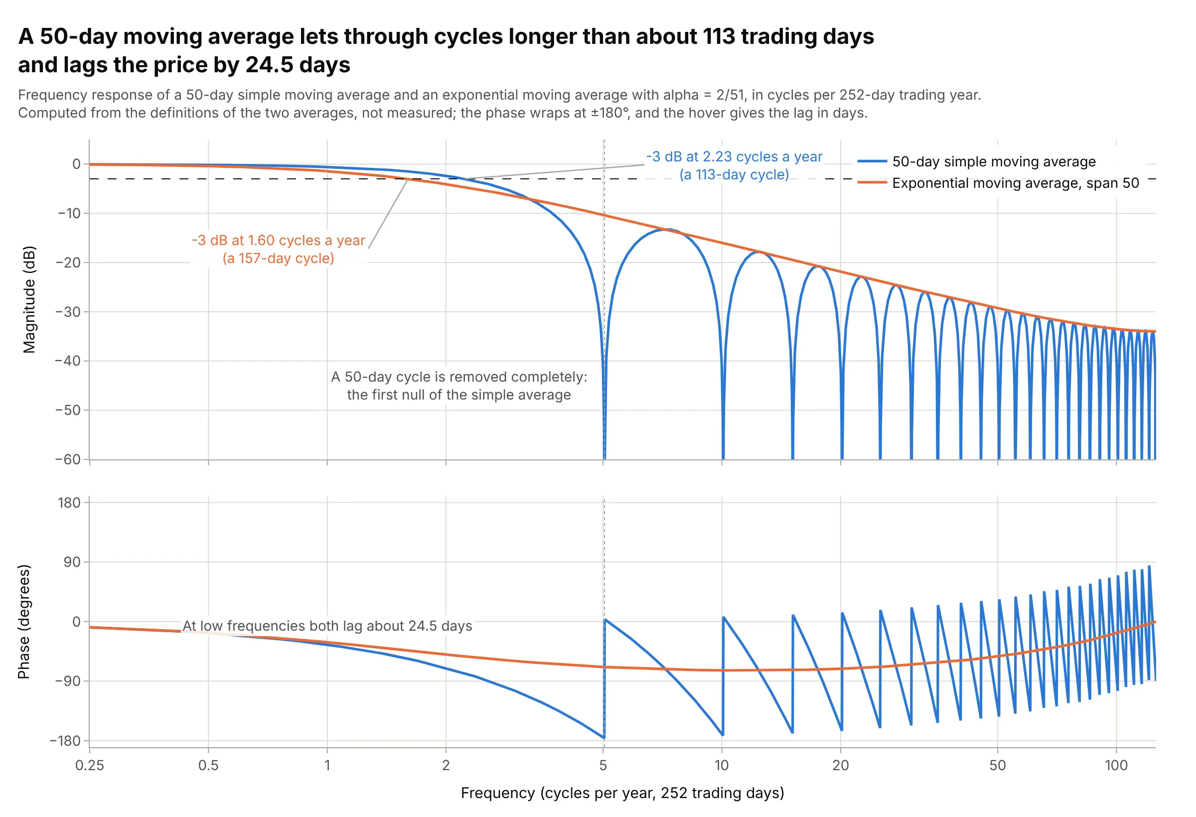
Bode plot of a 50-day simple moving average and an exponential moving average against cycles per trading year: the simple average is -3 dB at 2.23 cycles a year and has nulls every 5.04 cycles a year, starting with the 50-day cycle; the exponential average falls smoothly and is -3 dB at 1.60 cycles a year

Traders draw moving averages as trend lines, but a 50-day simple moving average is a low-pass filter: it lets through cycles longer than about 113 trading days within 3 dB, removes a 50-day cycle completely, and lags the price by 24.5 days. An exponential average with the same span has no nulls and the same low-frequency lag. Data: computed from the definitions of the two averages, not measured.

Tip: label the frequency axis in units the audience uses, here cycles per 252-day trading year.

Make a plotly Bode plot of a 50-day simple moving average and an exponential moving average (alpha = 2/51),
computed from their definitions, against frequency in cycles per 252-day trading year from 0.25 to 126.

Magnitude in dB and phase in degrees with a shared log x axis, a -3 dB line, a dotted line at the 50-day cycle,
and the lag in days in the phase hover.

6. A lithium-ion cell’s impedance as it ages

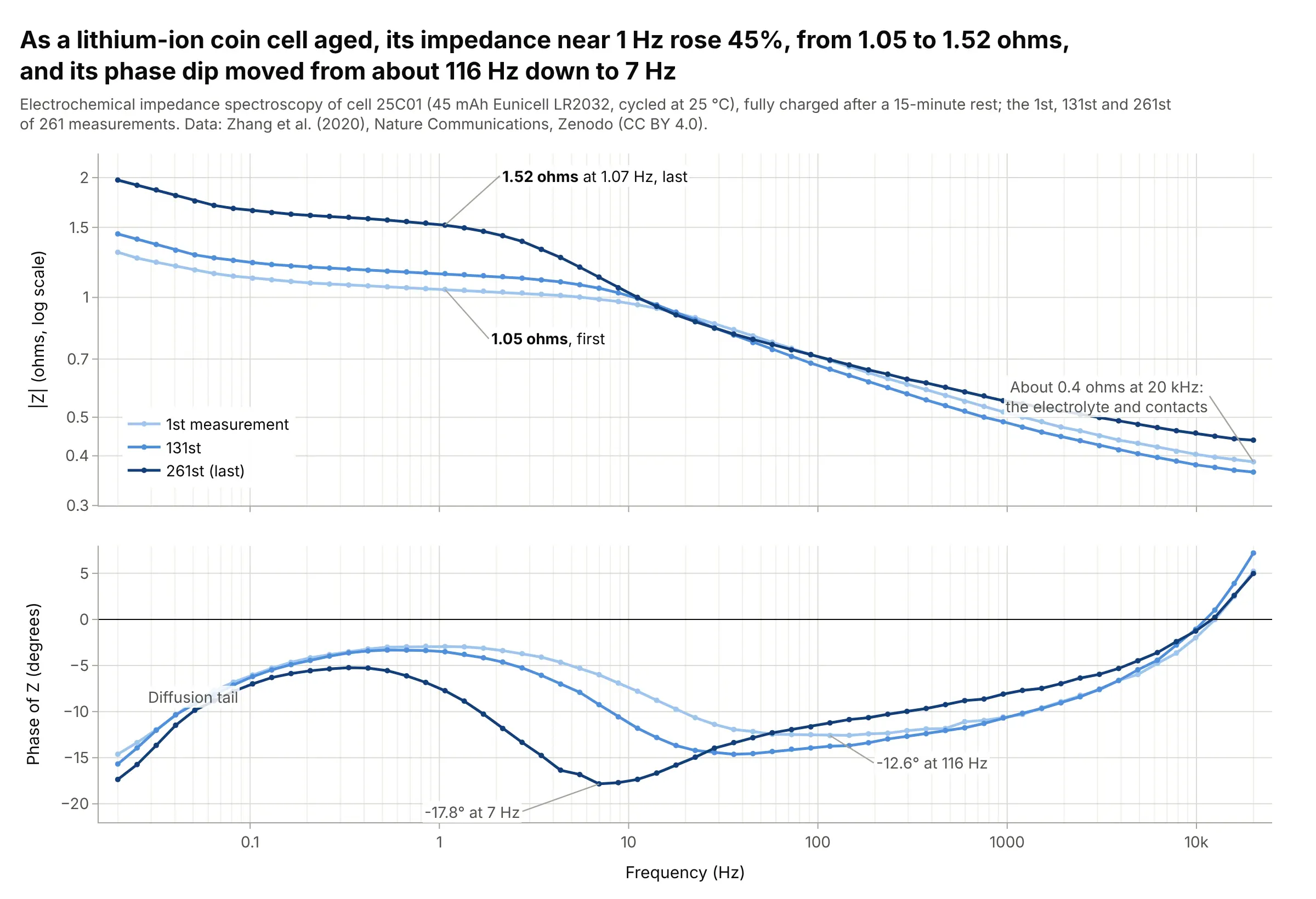
Bode plot of a lithium-ion coin cell’s impedance for its 1st, 131st, and 261st measurements from 0.02 Hz to 20 kHz: impedance in ohms on a log axis rises at low frequency from 1.05 to 1.52 ohms near 1 Hz, and the phase dip moves from -12.6 degrees at 116 Hz to -17.8 degrees at 7 Hz

In electrochemical impedance spectroscopy (EIS), Bode plots show how a battery’s impedance depends on frequency. As one 45 mAh coin cell aged, its impedance near 1 Hz rose 45%, from 1.05 to 1.52 ohms, and its phase dip moved from about 116 Hz to 7 Hz, while the impedance at 20 kHz, usually read as the electrolyte and contacts, stayed near 0.4 ohms. Data: Zhang et al. (2020), Nature Communications, Zenodo (CC BY 4.0).

Tip: EIS plots |Z| in ohms on a log axis instead of dB; use a light-to-dark scale for measurements over time.

Get the data from Zenodo record 3633835 (Zhang et al. 2020, "Identifying degradation patterns of lithium ion
batteries from impedance spectroscopy", EIS data.zip, file EIS_state_V_25C01.txt: time, cycle number, freq/Hz,
Re(Z), -Im(Z), |Z|, Phase(Z)) and keep the 1st, 131st, and 261st spectra (columns: measurement, freq_hz, abs_z_ohm,
phase_deg).

Make a plotly Bode plot with |Z| on a log y axis in ohms and phase in degrees, a shared log x axis, and the three
measurements in a light-to-dark blue scale.

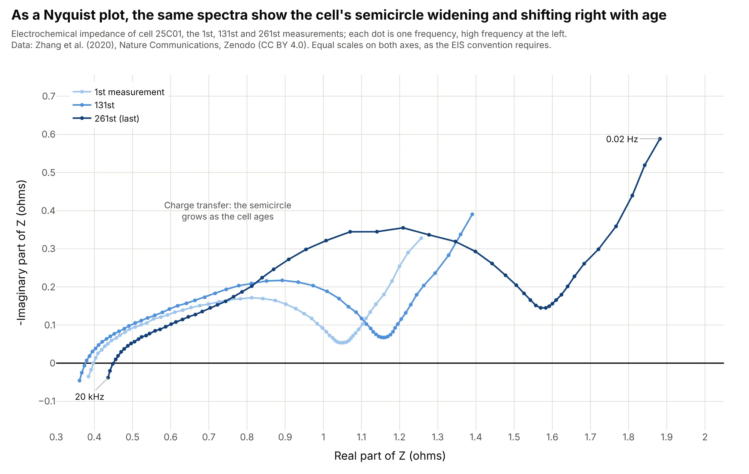
Another way to see it: electrochemists more often draw the same spectra as a Nyquist plot, where the charge-transfer semicircle grows and shifts right as the cell ages, but frequency is only a label on each dot.

Nyquist plot of the same three impedance spectra, real part against minus the imaginary part in ohms on equal scales: each curve is a depressed semicircle followed by a rising diffusion tail, and the last measurement’s semicircle is larger and further right, ending at 0.02 Hz near 1.9 ohms

7. A headphone’s measured response against the Harman target

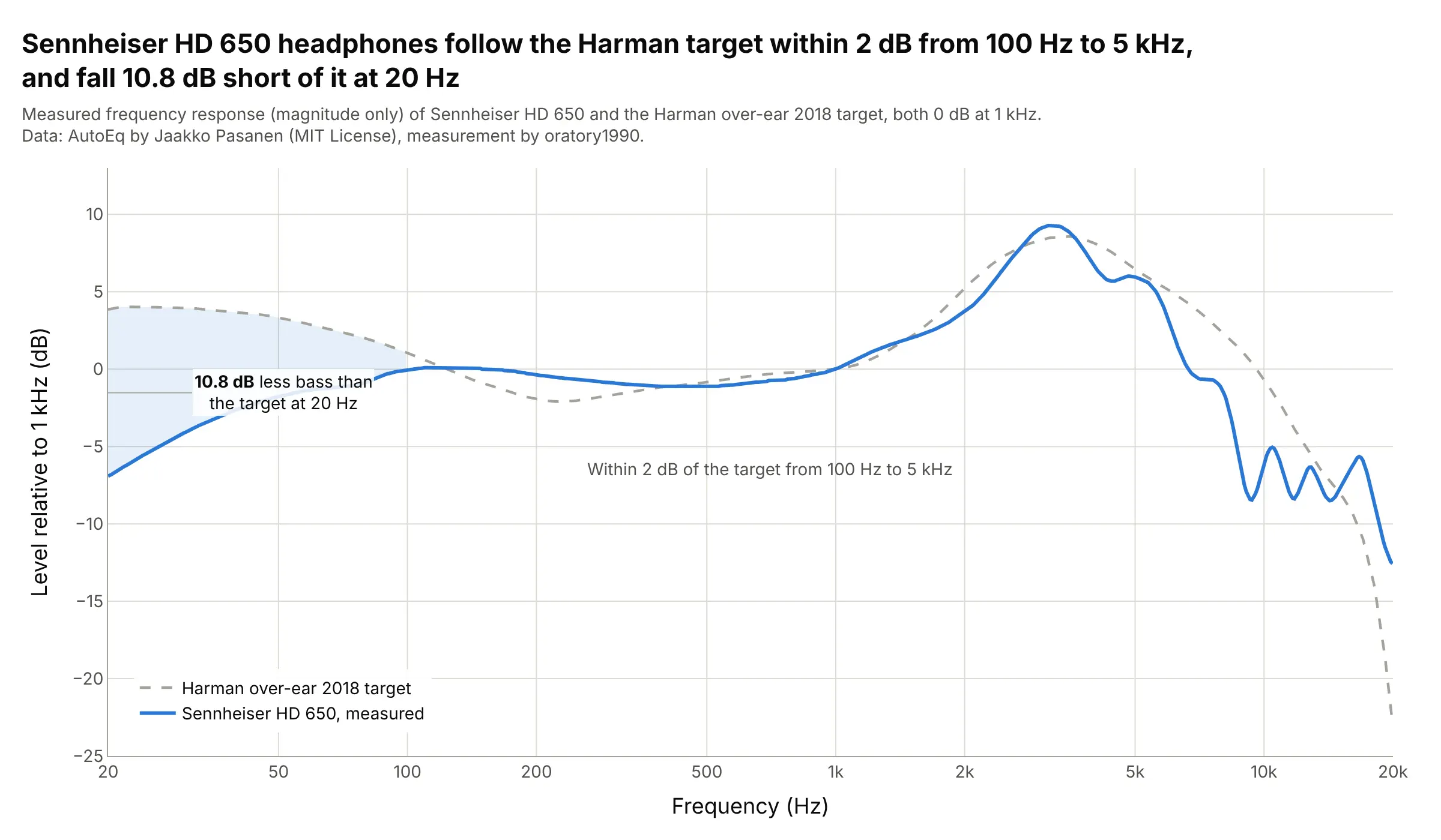
Measured frequency response of Sennheiser HD 650 headphones and the Harman over-ear 2018 target from 20 Hz to 20 kHz, both 0 dB at 1 kHz: the two lines stay within 2 dB from 100 Hz to 5 kHz, the headphones fall 10.8 dB below the target at 20 Hz, shaded, and both have a peak near 3 kHz

Audio frequency responses are usually the magnitude half of a Bode plot, from 20 Hz to 20 kHz on a log axis. Sennheiser HD 650 headphones stay within 2 dB of the Harman over-ear target from 100 Hz to 5 kHz and fall 10.8 dB short of it at 20 Hz, a bass shortfall that equalizers like AutoEq correct. Data: AutoEq by Jaakko Pasanen (MIT License), measurement by oratory1990.

Tip: draw the target as a dashed gray line and shade the gap that matters.

Get the data from the AutoEq repository on GitHub (jaakkopasanen/AutoEq: measurements/oratory1990/data/over-ear/
Sennheiser HD 650.csv and targets/Harman over-ear 2018.csv, columns frequency, raw in dB).

Make a plotly frequency response plot from 20 Hz to 20 kHz on a log x axis ticked 20, 50, 100 ... 20k, the target
dashed gray, the measurement in blue, and the gap below 100 Hz shaded and labeled.