Parallel Categories Diagrams - A Complete Guide

TL;DR

• A parallel categories diagram draws one vertical axis per categorical column, a box on each axis per category sized by its count, and ribbons between neighboring axes whose width is the number of records with that combination of categories.
• Parallel categories diagrams are also known as parallel sets, parallel categories plots and alluvial diagrams (or alluvial plots, in R's ggalluvial), and are similar to Sankey diagrams, parallel coordinates plots and Marimekko charts.
• Use one for three to five categorical columns with a handful of categories each, when the question is how the categories combine: who survived in which class, which applications in which loan type were denied, which counties switched party and when.
• You can make one with Plotly in one line of code with px.parallel_categories, or with go.Parcats (the parcats trace) and its counts argument when your table is already aggregated.

What is a parallel categories diagram?

Parallel categories diagrams look like this:

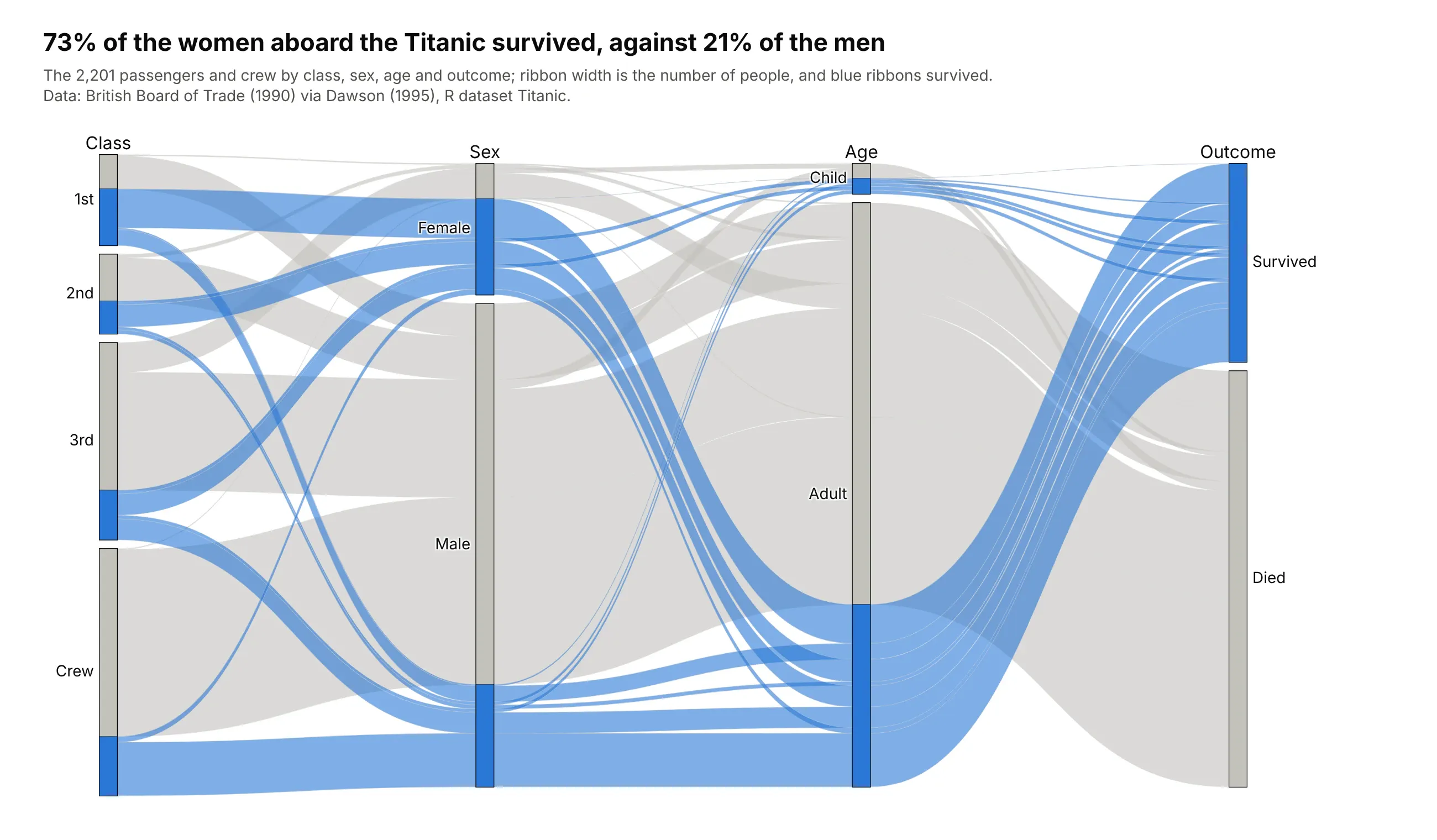
Data: British Board of Trade (1990) via Dawson (1995), R dataset Titanic.

How do you read a parallel categories diagram? In the example above, notice these things:

• Each vertical axis is one column of the table, and each box on it is a category whose height is its share of the 2,201 people. The crew is the tallest box on the class axis, with 885 people, more than any class of passengers.
• Ribbons run between neighboring axes, and a ribbon's thickness is the number of people with that pair of categories. The ribbons from Crew to Male hold 862 of the 885 crew members.
• The color comes from the outcome axis and is carried back along every ribbon, so each box splits into survived (blue) and died (gray). 141 of the 145 women in first class survived, against 90 of the 196 women in third class.
• Comparing the blue part of two boxes on one axis compares survival rates: 73% of women survived and 21% of men, and every one of the 30 children in first and second class survived.
• Only neighboring axes are joined by ribbons, so the order of the axes decides which combinations you can follow directly. Here sex sits next to class, so the class-by-sex split is easy to read.

It's often used for charts like these:

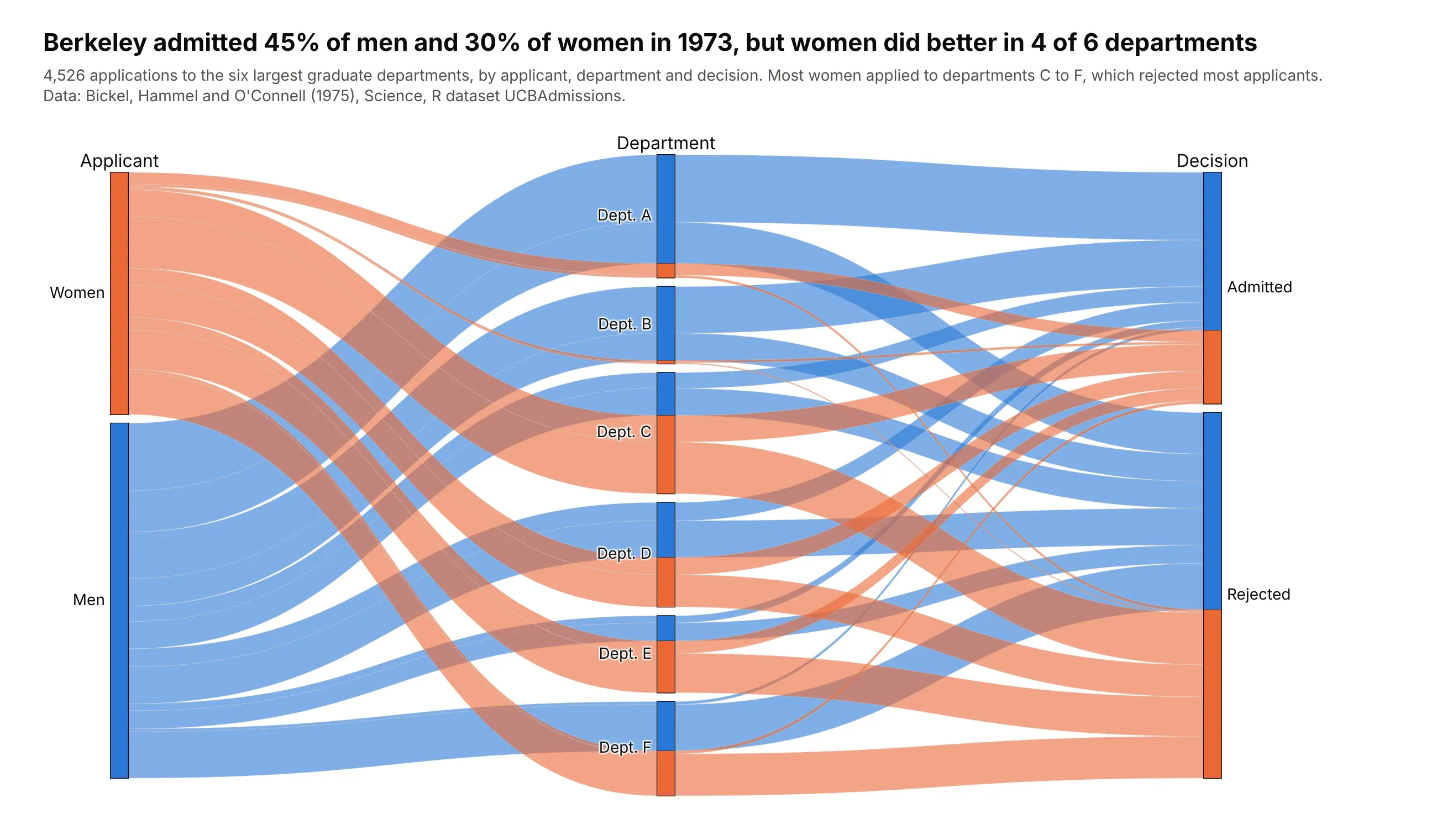
Survey and admissions crosstabs. Berkeley admitted 45% of men and 30% of women in 1973, yet women had the higher admission rate in 4 of 6 departments, because 93% of women applied to the four departments that rejected most applicants. Data: Bickel, Hammel and O'Connell (1975), R dataset UCBAdmissions.

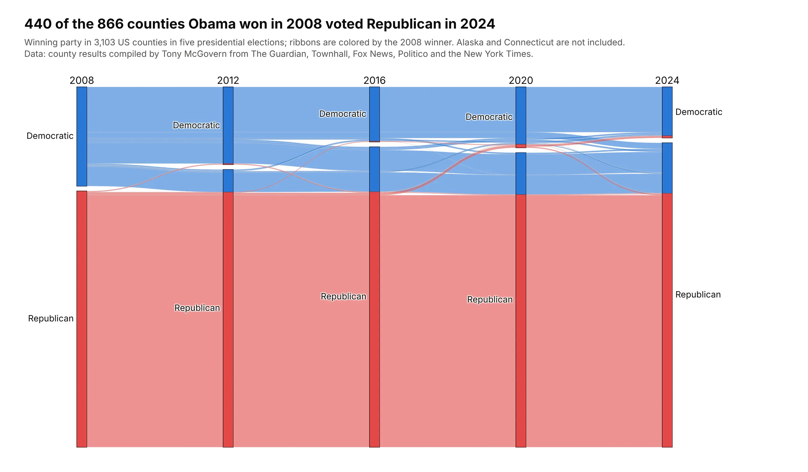
Voter shifts over time (alluvial diagrams). With one axis per election, the ribbons follow the same counties through time: 440 of the 866 counties Obama won in 2008 voted Republican in 2024, while 19 counties went the other way. Data: county results compiled by Tony McGovern.

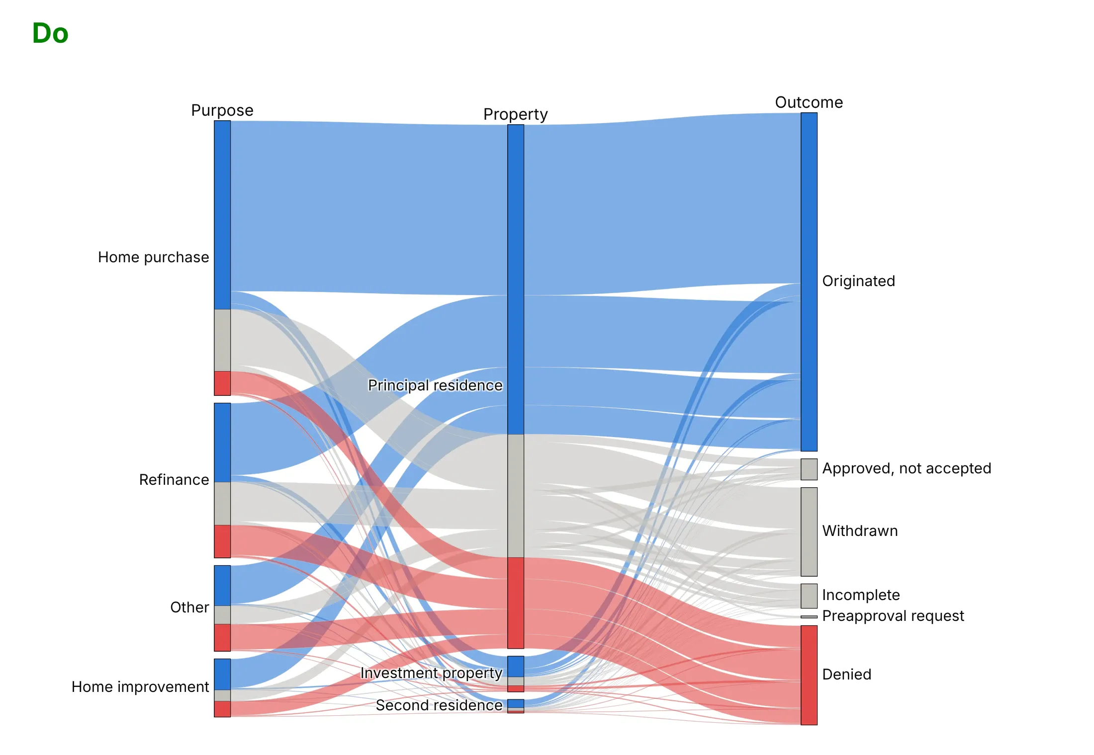
Outcomes in big transaction tables. Colorado lenders denied 9% of home purchase applications in 2024 and 27% of home improvement ones, and the debt-to-income ratio was the most common reason, behind 15,944 of 41,927 denials. Data: CFPB and FFIEC, HMDA Data Browser.

A short history

Fabian Bendix, Robert Kosara and Helwig Hauser introduced Parallel Sets for categorical data at IEEE InfoVis in 2005 (Bendix et al. 2005) and published an expanded version in 2006 (Kosara et al. 2006), which shows frequencies instead of individual records and was demonstrated on a large customer dataset and on housing data from two US states. Kosara later called the people on board the Titanic "my standard example", which is the chart at the top of this page. Alluvial diagrams come from network science, where Rosvall and Bergstrom used them to show how the fields in a citation network of about 7,000 scientific journals changed between 2001 and 2007 (2010). R's ggalluvial package (Brunson 2020) applies the same idea to frequency tables of several categorical variables and to answers that change over time. plotly.js added the parcats trace in version 1.42.0 in October 2018.

Alternatives to a parallel categories diagram

Here's the Titanic table (class, sex and outcome) drawn six ways. Some are better for the question, some worse, some just different:

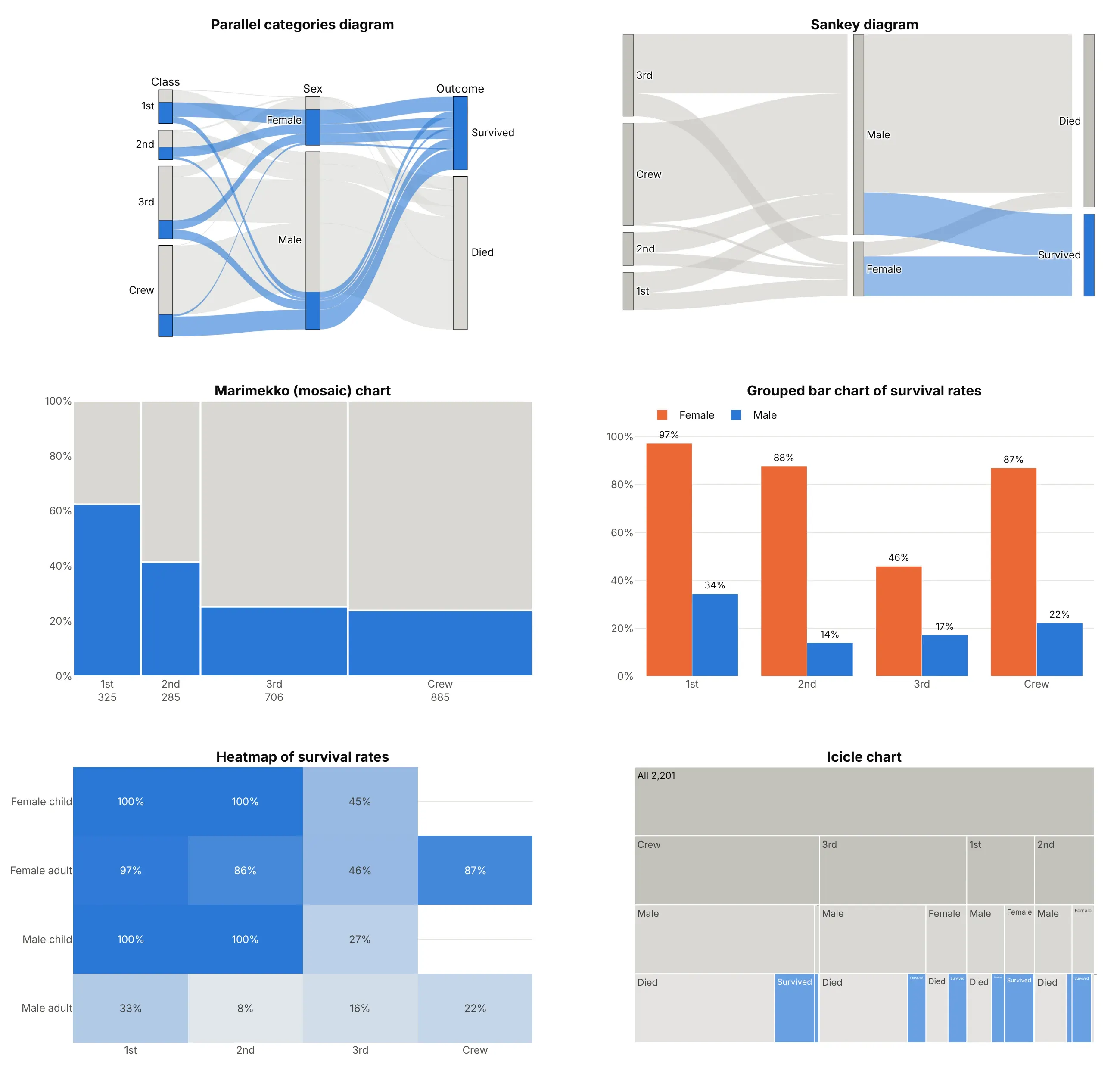
• Sankey diagram (different). A Sankey draws nodes and the flows between them, and each link only knows its two ends, so once the ribbons meet at the Male node you can no longer tell which class they came from. A parallel categories diagram draws dimensions instead of nodes and keeps every record's path, so when you color it by class (as in the dos and don'ts below), each class's ribbons can be followed past the Sex axis to the outcome. Use a Sankey for flows such as energy or money, where only the pairwise links exist.
• Marimekko chart (better for two columns). Widths for class size and heights for the survival share show both numbers at once and read more exactly than ribbons, but a third column means splitting every bar again.
• Grouped bar chart of rates (better for comparing rates). If the question is "who survived?", bars of the survival rate by class and sex (97% of first-class women, 14% of second-class men) are the most exact answer, though the group sizes disappear.
• Heatmap (better for precise rates). A grid of rates by class and by sex and age holds every combination with its number printed, which suits many small groups, but it shows rates without counts.
• Icicle chart (works too, for a strict hierarchy). Nesting class, then sex, then outcome gives every combination a rectangle, but the same categories repeat in every branch, so "all women" is spread over four places. A treemap or sunburst has the same trade-off.

The Titanic table has no numeric columns, so one relative is missing from the figure. A parallel coordinates plot has the same parallel axes, but each axis is a numeric scale and each record is its own line, so use it when the columns are measurements and a parallel categories diagram when they are categories.

How to make a parallel categories diagram

With AI

ChatGPT, Claude Code, GitHub Copilot, Cursor and other AI tools are excellent at writing Plotly code. Name Plotly in the prompt, and say which column goes on which axis, in what order the categories should be, and what the color follows:

With Plotly Studio

Plotly Studio is a desktop app where you point an AI at a dataset and it builds charts and a Dash app around your questions. Ask for a parallel categories diagram the same way:

Show a parallel categories diagram of mortgage applications by purpose, loan type and outcome, with ribbons sized by the number of applications, approved loans in blue and denials in red, and a filter for the year.

Make a parallel categories diagram in Python or JavaScript

This is the code AI tools write under the hood. In Python, go.Parcats takes one dict per axis and, with counts, a table that is already aggregated, and the Plotly parallel categories documentation has more examples:

With one row per record, px.parallel_categories(df, dimensions=["class", "sex", "age", "survived"], color="survived_num") does the counting for you in one line of code. Its color takes a numeric column, so map a category to numbers first (as above) and pick a two- or few-color color_continuous_scale. Without dimensions, it uses every column with 50 or fewer distinct values.

In JavaScript, plotly.js draws the same thing with a parcats trace:

Share it

Every Plotly chart has a Share chart button (the cloud icon in its toolbar) that uploads it to Plotly Cloud and gives you a link. Only you can see it until you change its visibility.

For a live app, put the chart in a Dash app and publish it with the Plotly Cloud CLI. Coding agents can run these commands for you:

If your data has to stay in your own cloud or data center, publish to Dash Enterprise instead.

Dos and don'ts

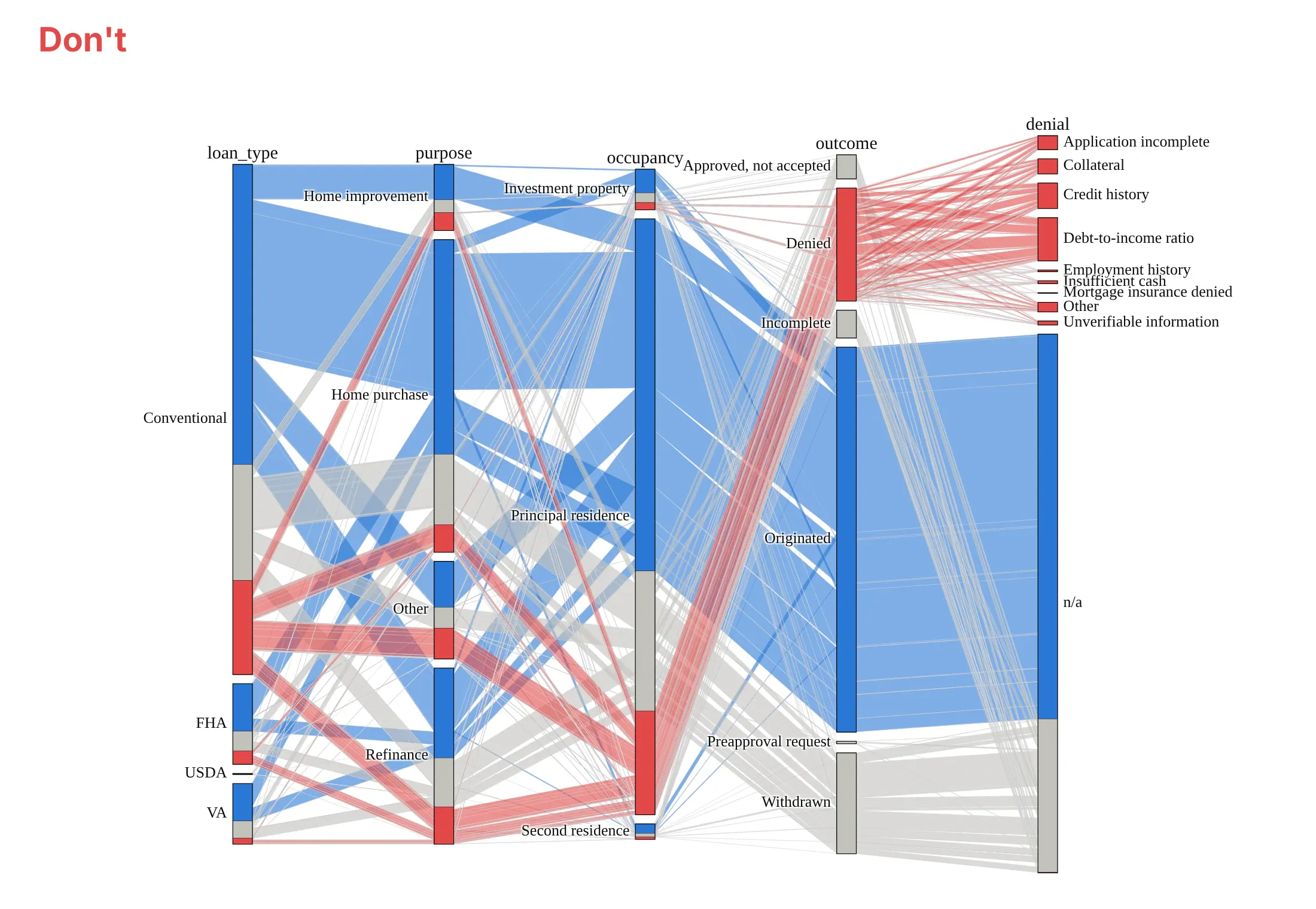
Most of the work in a published parallel categories diagram is choosing a few columns, ordering the categories and keeping the labels readable. Here are Colorado's 242,294 mortgage applications both ways, with the same colors.

Don't add every column you have (here five, with ten denial categories), leave the categories in alphabetical order, use raw column names such as loan_type as axis labels, or keep a default serif font, because the ribbons tangle and the small categories' labels pile on top of each other:

Do keep the three columns that answer one question, order categories by size (or by their natural order, like the outcome here), name the axes in plain words and curve the ribbons:

Choose what the color follows

The color is the one thing a reader can follow across every axis, so give it to the column the question is about. Colored by outcome (the chart at the top of the page), the Titanic diagram answers "who survived?". Colored by class, the same data answers "what happened to each class?", and the third-class ribbons (orange) can be followed into the Died box:

Checklist

Do

• Keep to three to five axes with two to about eight categories each; group the rest as "Other".
• Order categories by their natural order (time, age bands, outcome) or by size, with categoryorder="array".
• Put the two columns you most want to compare next to each other, because only neighbors are joined.
• Color the ribbons by the column the question is about, with one highlight color and gray for the rest when one group matters most.
• Pre-aggregate big tables and pass counts, and keep the count and share in the hover label.
• Write a title that states the takeaway.

Don't

• Use a parallel categories diagram for numeric columns; cut them into a few meaningful bins or use parallel coordinates.
• Read ribbon crossings as meaningful; they come from the category order.
• Use it when the exact rates matter more than the paths; a bar chart or heatmap of rates is easier to read.

Options to customize

A parallel categories diagram in Plotly is a parcats trace, so these are the options that matter most. The full lists are in the parcats reference and the px.parallel_categories reference.

1. dimensions: one dict per axis with label and values, in the left-to-right order you want.
2. dimensions[].categoryorder, categoryarray: the order of the categories on an axis; "array" with a list for ordinal categories, or "category ascending".
3. dimensions[].ticktext: display names for the categories in categoryarray, when the data has codes.
4. dimensions[].displayindex: the axis position, if you want to reorder axes without reordering the list.
5. counts: the number of records each row stands for (people, applications, gigawatts); defaults to 1.
6. line.color, line.colorscale: ribbon color, a number per row mapped through a colorscale; use a stepped scale for categories.
7. line.shape: "hspline" for curved ribbons, "linear" (the default) for straight ones.
8. bundlecolors: keeps ribbons of the same color together inside each category (on by default).
9. sortpaths: "forward" (default) or "backward", which ribbons are sorted by when they leave a category.
10. arrangement: how readers can drag categories and axes to untangle the ribbons: "perpendicular" (default) along a line across the ribbons, "freeform" anywhere, or "fixed" not at all.
11. hoveron, hoverinfo, line.hovertemplate: what the hover label is attached to ("category", "color" or "dimension") and whether it shows the count, the probability or both.
12. labelfont, tickfont, domain: axis title and category label fonts, and the area the diagram takes up (leave room on the left for the first axis's labels).
13. px.parallel_categories(color=..., color_continuous_scale=..., dimensions_max_cardinality=...): the Plotly Express version, which counts rows for you and skips columns with more distinct values than the limit (50).

More parallel categories diagram examples

Seven more parallel categories diagrams built from real public data, each with its source, the technique that makes it work and a prompt to rebuild it. Several use the textbook datasets these diagrams are best known for, from R's built-in datasets and the ggalluvial package.

1. Flu vaccination intentions in three surveys (ggalluvial's example)

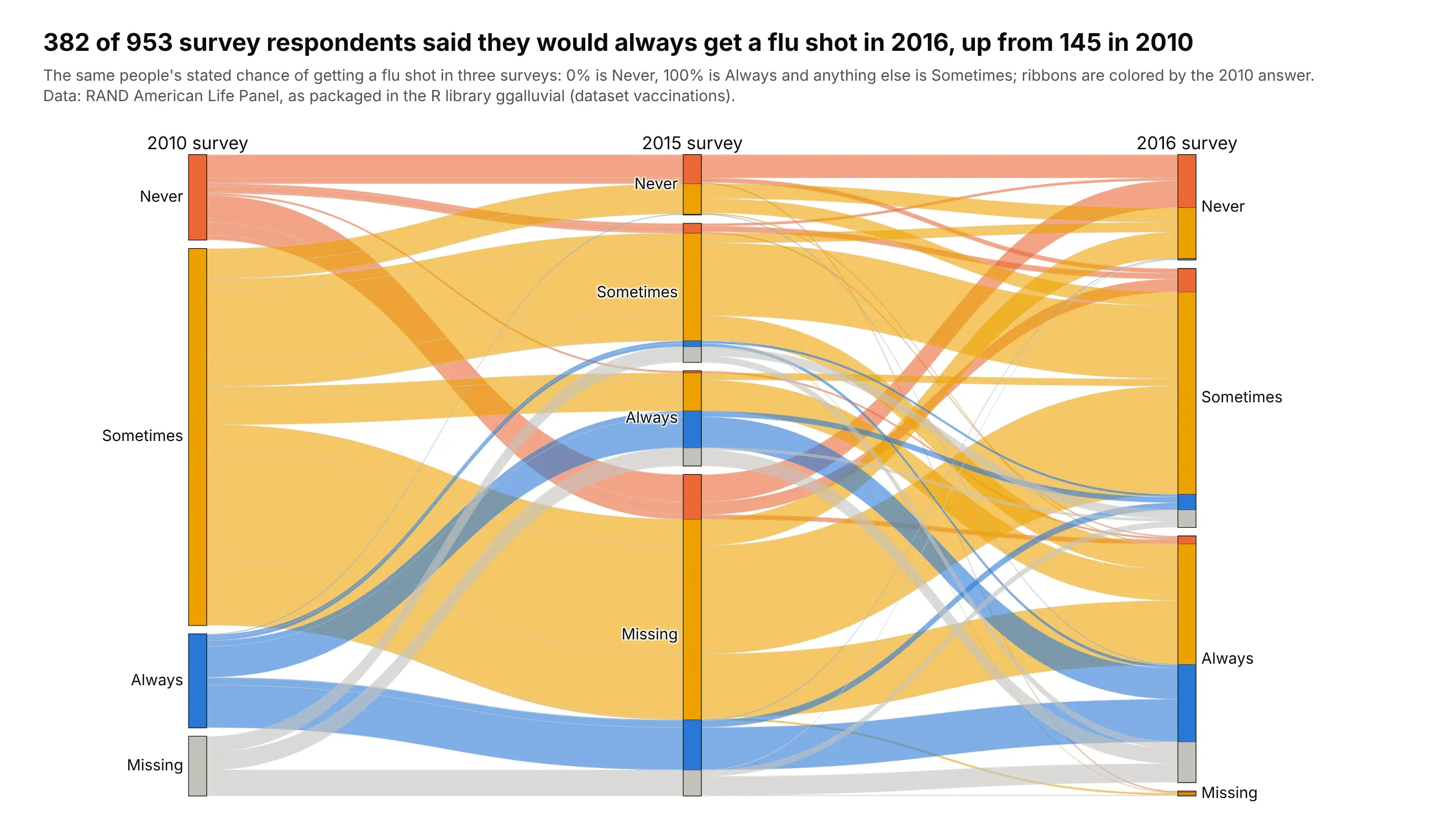
382 of 953 respondents said they would always get a flu shot in 2016, up from 145 in 2010, and the ribbons show that 187 of them had said Sometimes in 2010. Only 198 gave the same answer all three times. Data: RAND American Life Panel, via the vaccinations dataset in R's ggalluvial.

Tip: for repeated surveys, give each wave its own axis with the same category order, and color by the first wave so changes stand out.

2. The US power plant pipeline

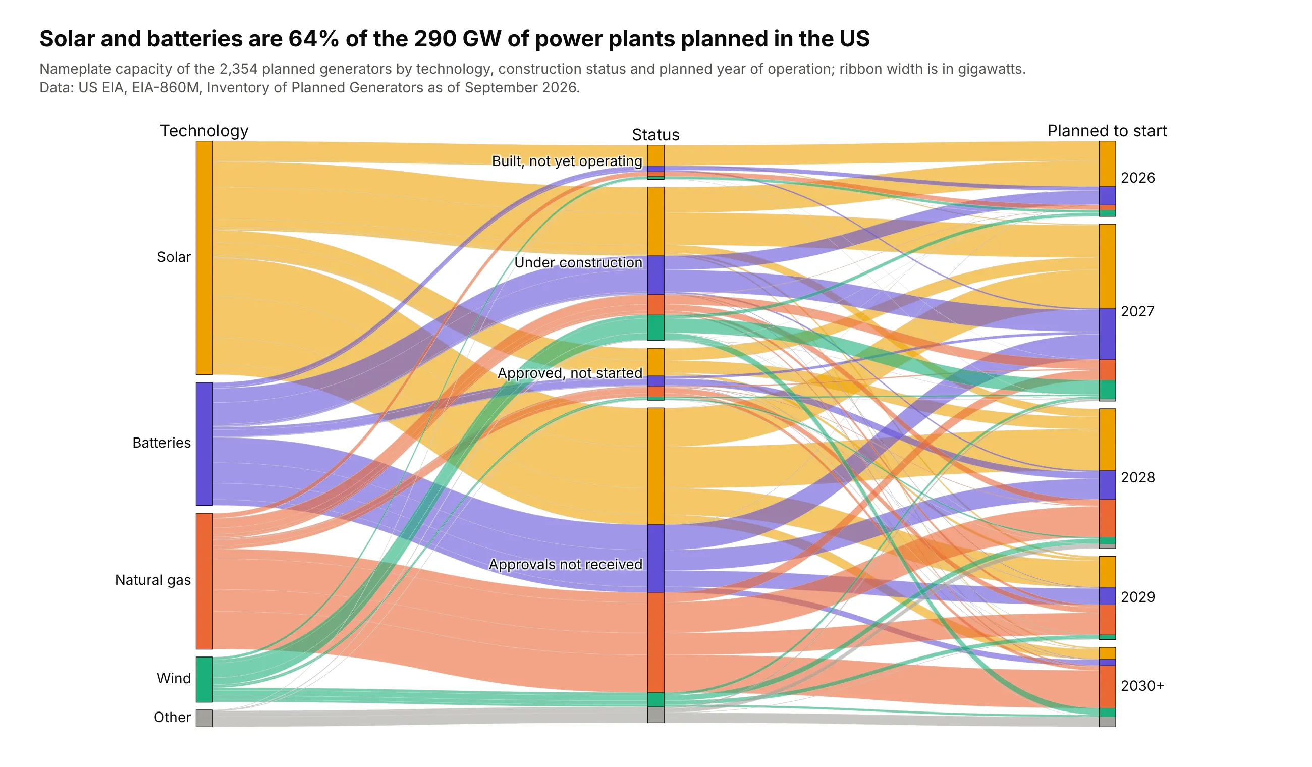
Solar and batteries are 64% of the 290 GW of generating capacity planned in the US, and 74% of the planned natural gas capacity has no regulatory approvals yet. The ribbons are sized in gigawatts, not generators. Data: US EIA, EIA-860M, September 2026.

Tip: pass a physical quantity to counts (here GW) when the number of rows would mislead, because one large gas plant outweighs many small solar farms.

3. Who reports GLP-1 side effects to the FDA

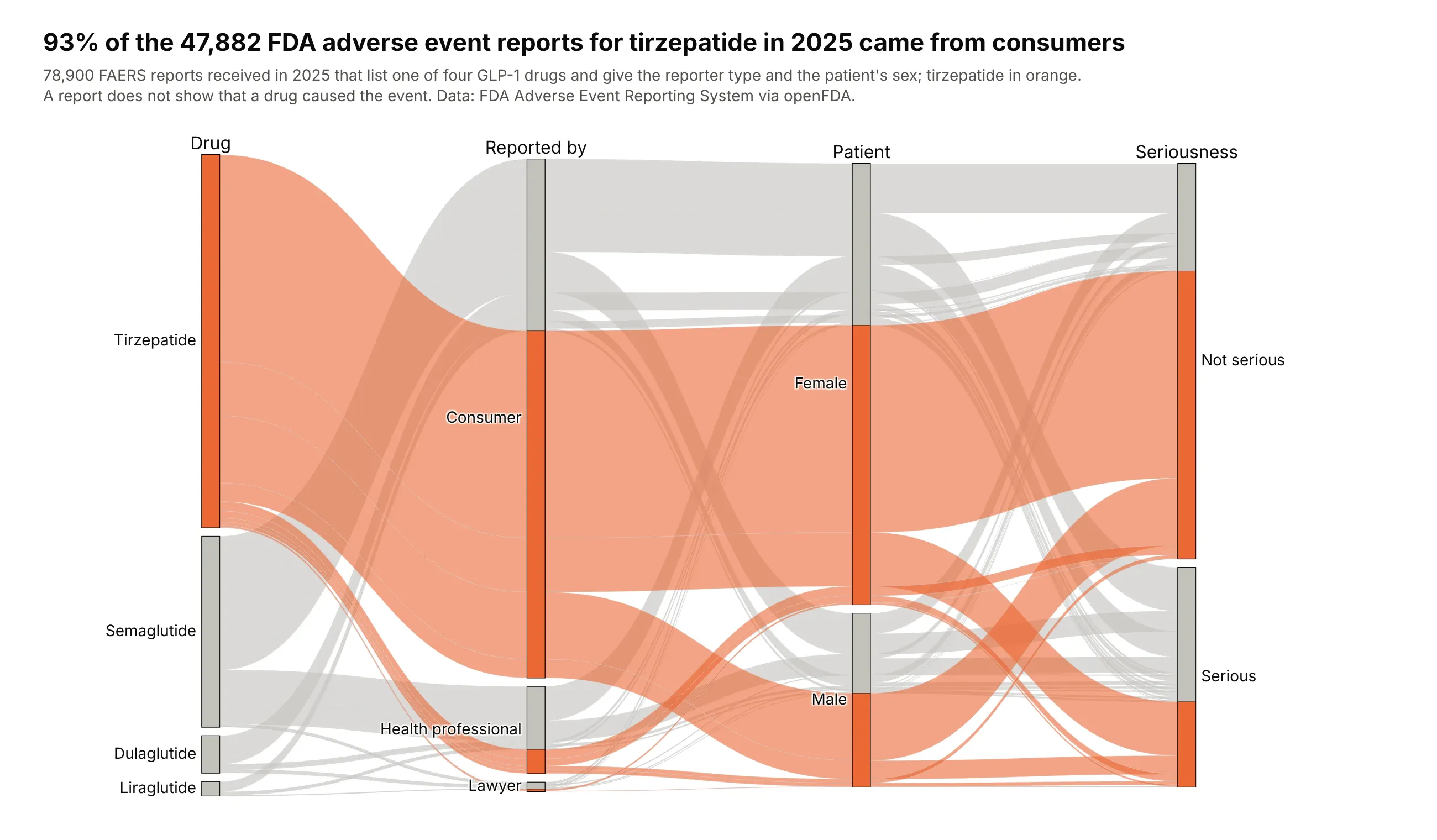
93% of the 47,882 adverse event reports for tirzepatide received in 2025 came from consumers, and 23% were marked serious, against 57% for semaglutide. A report shows that someone reported an event, not that the drug caused it. Data: FDA Adverse Event Reporting System via openFDA.

Tip: to tell one group's story, color it and leave the rest gray, and sort the data so the highlighted ribbons are drawn last.

4. A rheumatoid arthritis trial

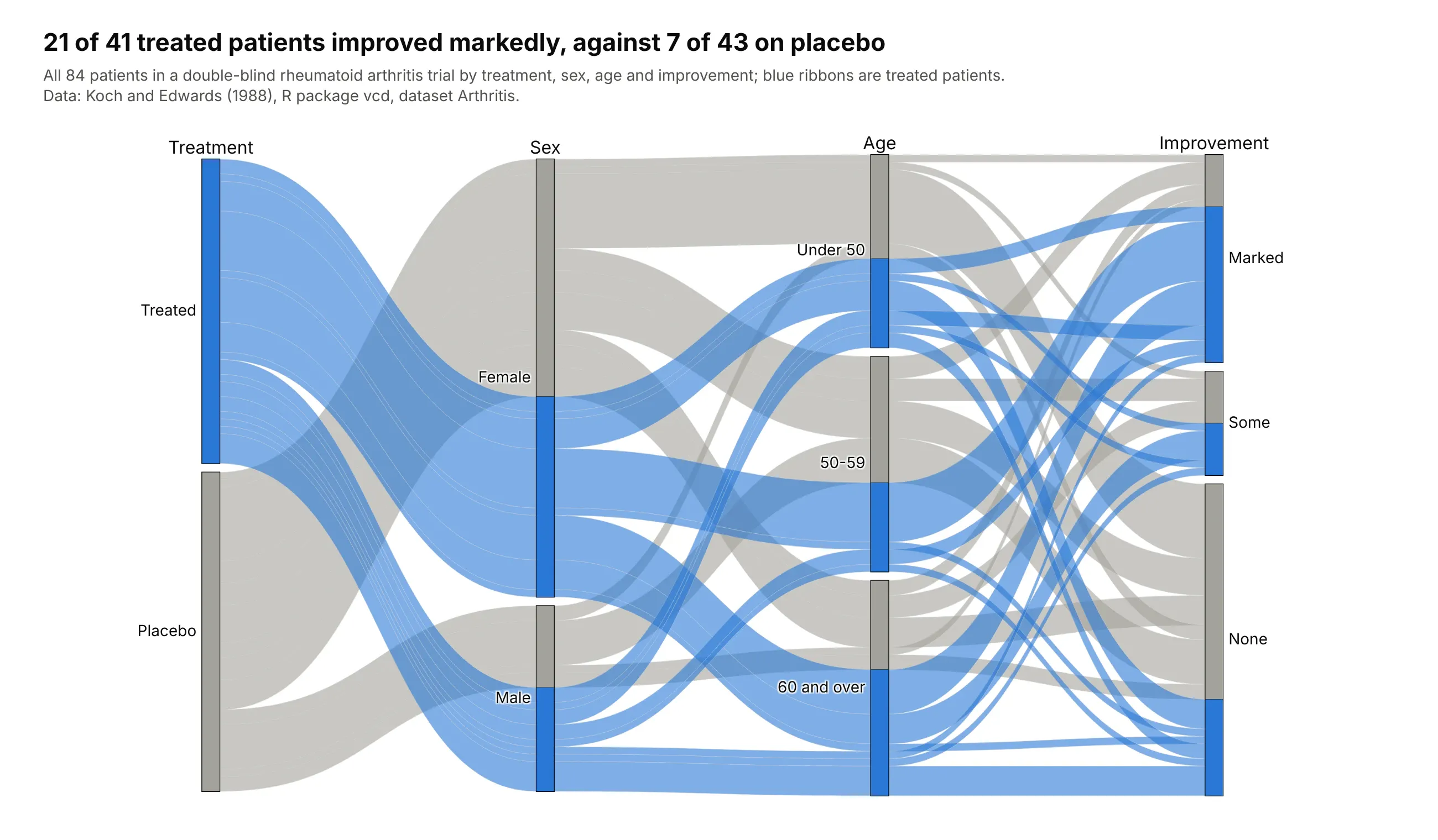
21 of 41 treated patients improved markedly, against 7 of 43 on placebo, and 29 placebo patients did not improve at all. With one row per patient, Plotly Express counts the combinations itself. Data: Koch and Edwards (1988), R package vcd, dataset Arthritis.

Tip: px.parallel_categories takes raw rows; pass a 0/1 column as color with a two-color scale and hide the colorbar.

5. Hair and eye color of 592 students

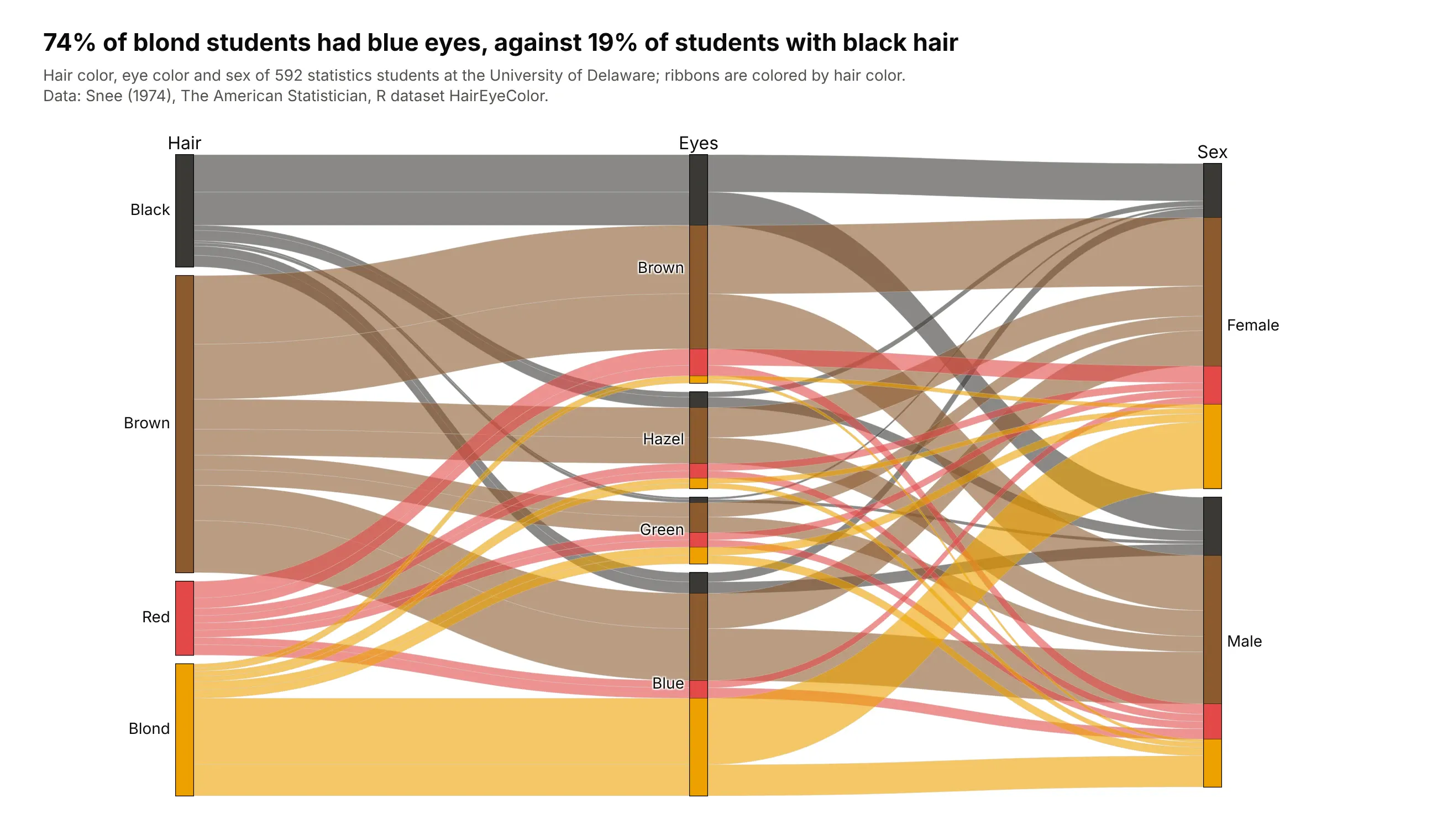
74% of blond students had blue eyes, against 19% of students with black hair, in the classic contingency table from a 1974 University of Delaware class. Brown hair with brown eyes was the largest group, 119 students. Data: Snee (1974), R dataset HairEyeColor.

Tip: when the categories have natural colors, use them for the ribbons and skip the legend.

6. The UCI mushroom dataset

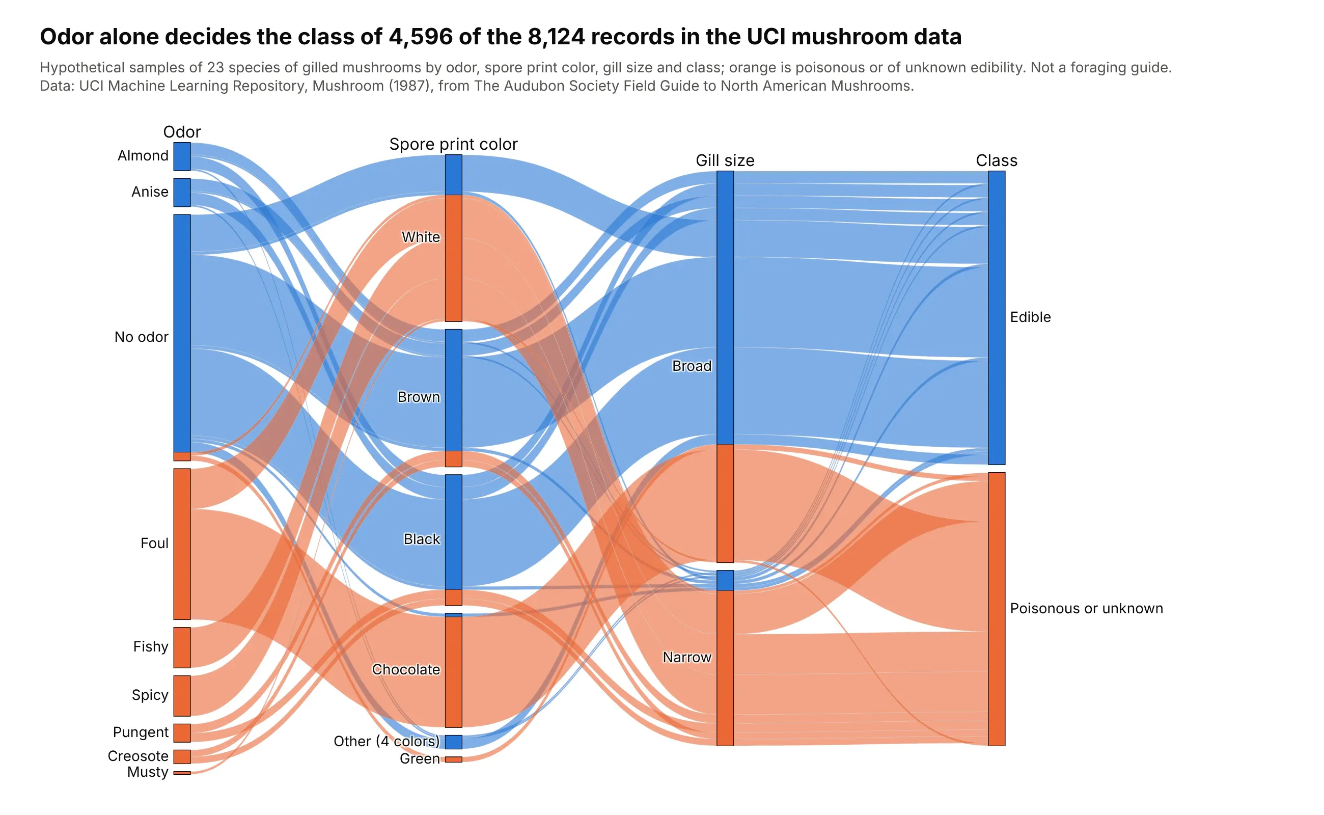
Odor alone decides the class of 4,596 of the 8,124 records: almond and anise are always edible, and any other smell is always poisonous or unknown. Of the 3,528 with no odor, 120 are poisonous or unknown, and the 72 of them with a green spore print are the only records with that color. The records are hypothetical samples, so this is not a foraging guide. Data: UCI Machine Learning Repository, Mushroom.

Tip: for a classification dataset, put the label last and color by it; any category whose ribbons are all one color decides the class by itself.

7. Who wins Nobel prizes

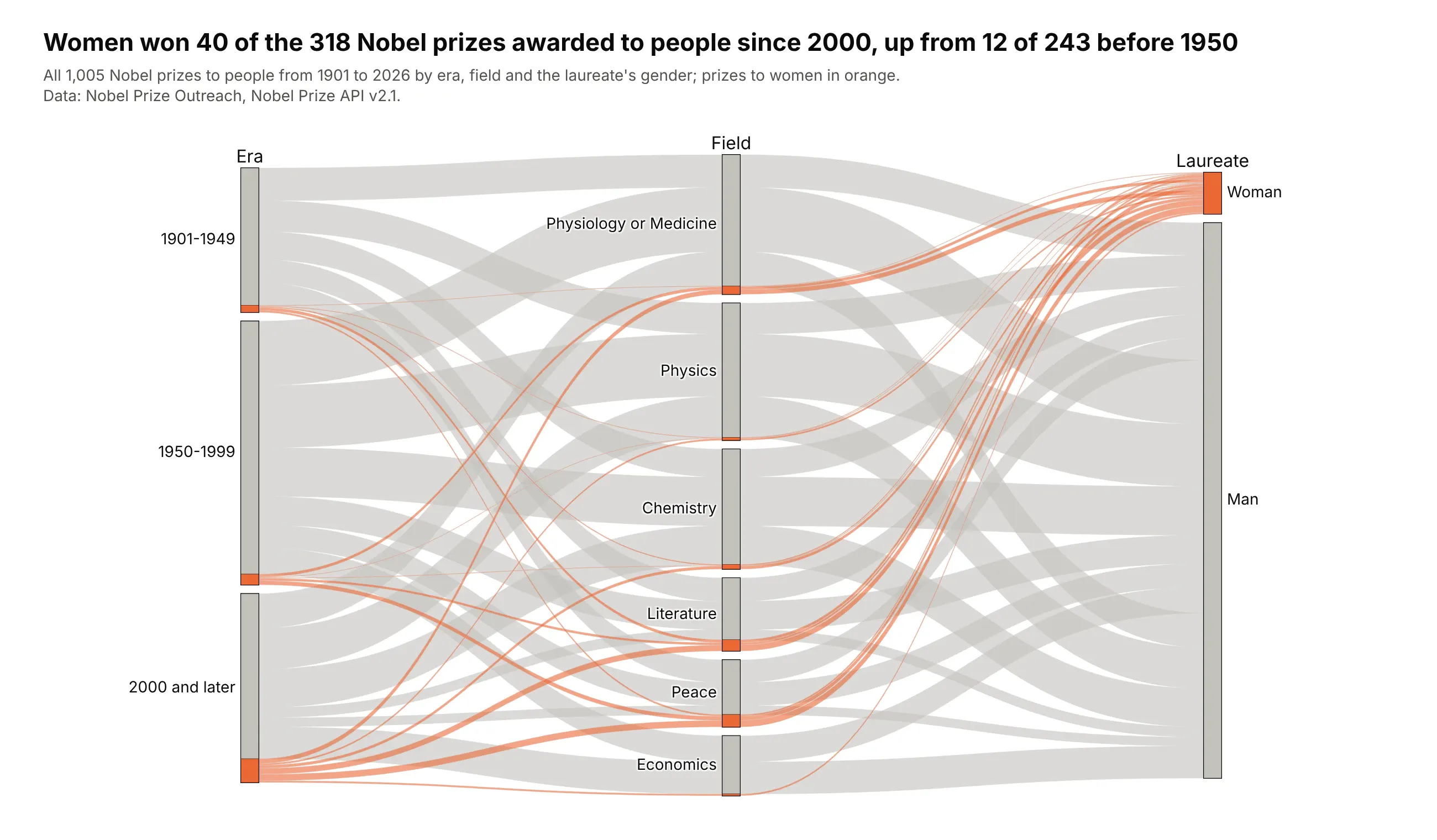
Women won 40 of the 318 Nobel prizes awarded to people since 2000, up from 12 of 243 before 1950, and 10 of the 27 literature prizes since 2000. Physics has gone to women 5 times in 231 prizes. Data: Nobel Prize Outreach, Nobel Prize API v2.1.

Tip: a small group gets lost in a bar chart of totals; color its ribbons and it stays visible on every axis.