Chris Parmer

October 24, 2026

Icicle Charts - A Complete Guide

TL;DR

An icicle chart draws a hierarchy as columns of adjacent bars: the root fills the first column, each level is one column further, and each bar's length is its share of the total.
Icicle charts are also known as icicle plots, and are similar to sunburst charts and treemaps.
A flame graph is an icicle chart of a CPU profile with the root at the bottom, which in Plotly is go.Icicle with tiling=dict(orientation="v", flip="y").
Use one when the reader follows paths through the levels (call stacks, code sets, budgets, file systems), and a sorted bar chart instead when there is only one level.
Any coding agent can make one with Plotly in a minute. In Python it's px.icicle(df, path=[...], values=...).

What is an icicle chart?

Icicle charts look like this:

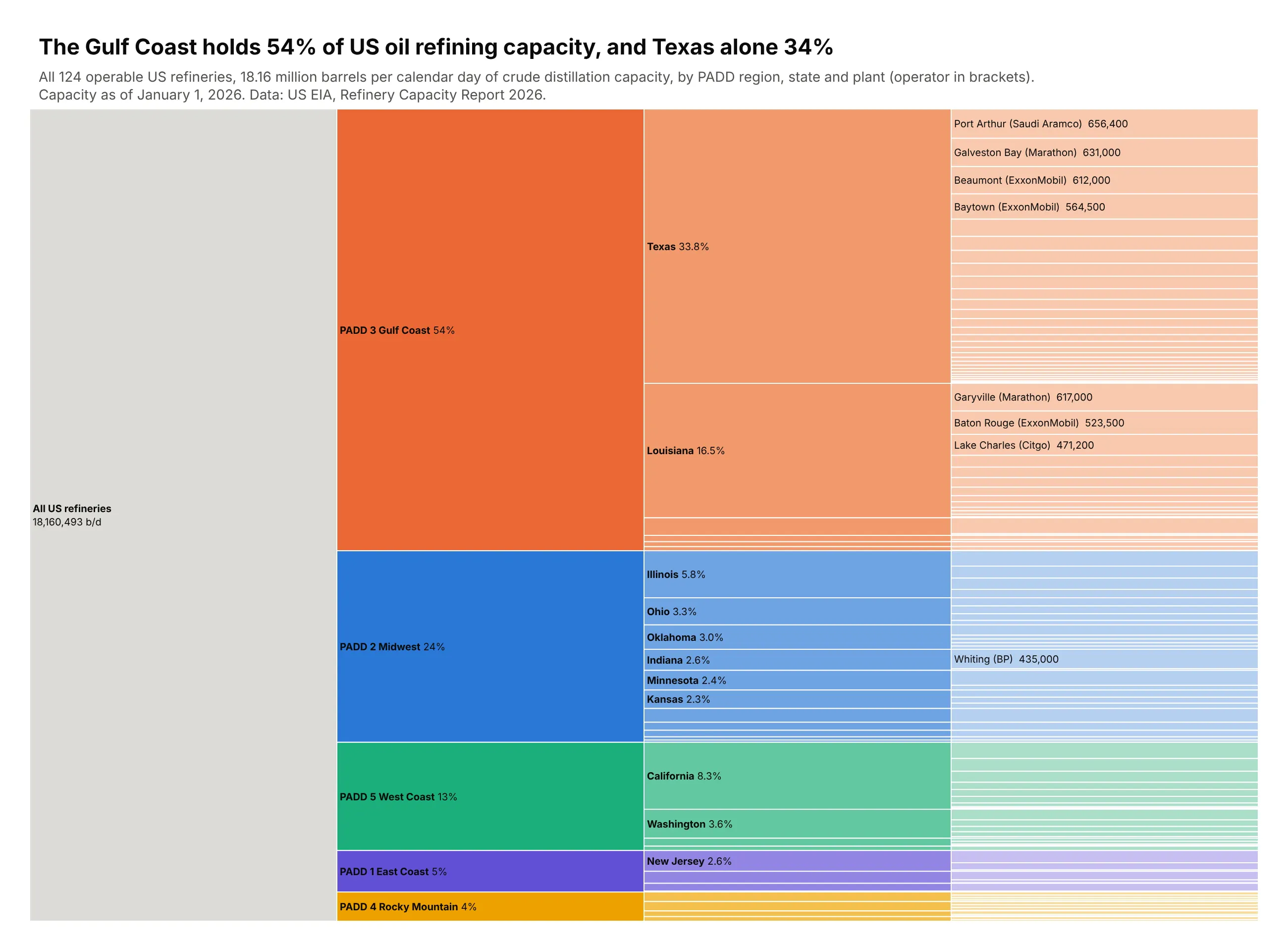
Horizontal icicle chart of all 124 US refineries by PADD region, state and plant. The Gulf Coast is 54% of the 18.16 million barrels per day, Texas 33.8%, and Port Arthur (Saudi Aramco) the largest plant at 656,400 barrels per day

Data: US EIA, Refinery Capacity Report 2026, capacity as of January 1, 2026.

How do you read an icicle chart? In the example above, notice these things:

The gray column on the left is the root, all US refining capacity, and each column to the right goes one level further down: PADD region, then state, then refinery.
A bar's height is its share of the total, so the orange Gulf Coast bar fills more than half the height of its column and Texas inside it about a third of the whole.
Every bar sits next to its parent, so you can follow a path from the total to a single plant in reading order, for example from the Gulf Coast through Texas to Port Arthur at the top right.
Each region keeps its color in lighter shades for its states and plants, and inside every parent the bars are sorted from largest at the top to smallest at the bottom, which is why the biggest plant of each state is the first one you see.
Most plant bars in the right column are too thin to label, so only the largest refineries like Whiting in Indiana are named, and you hover over a thin bar to read the rest.

It's often used for charts like these:

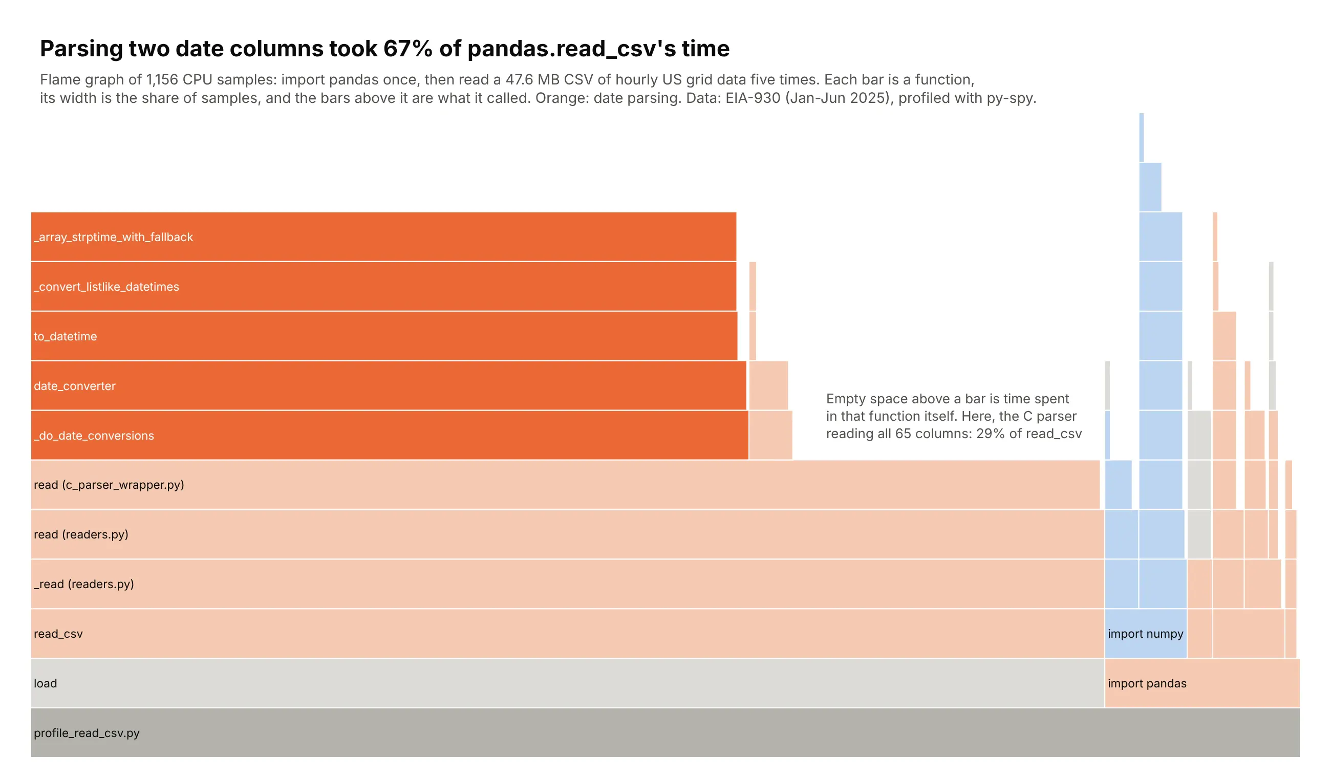
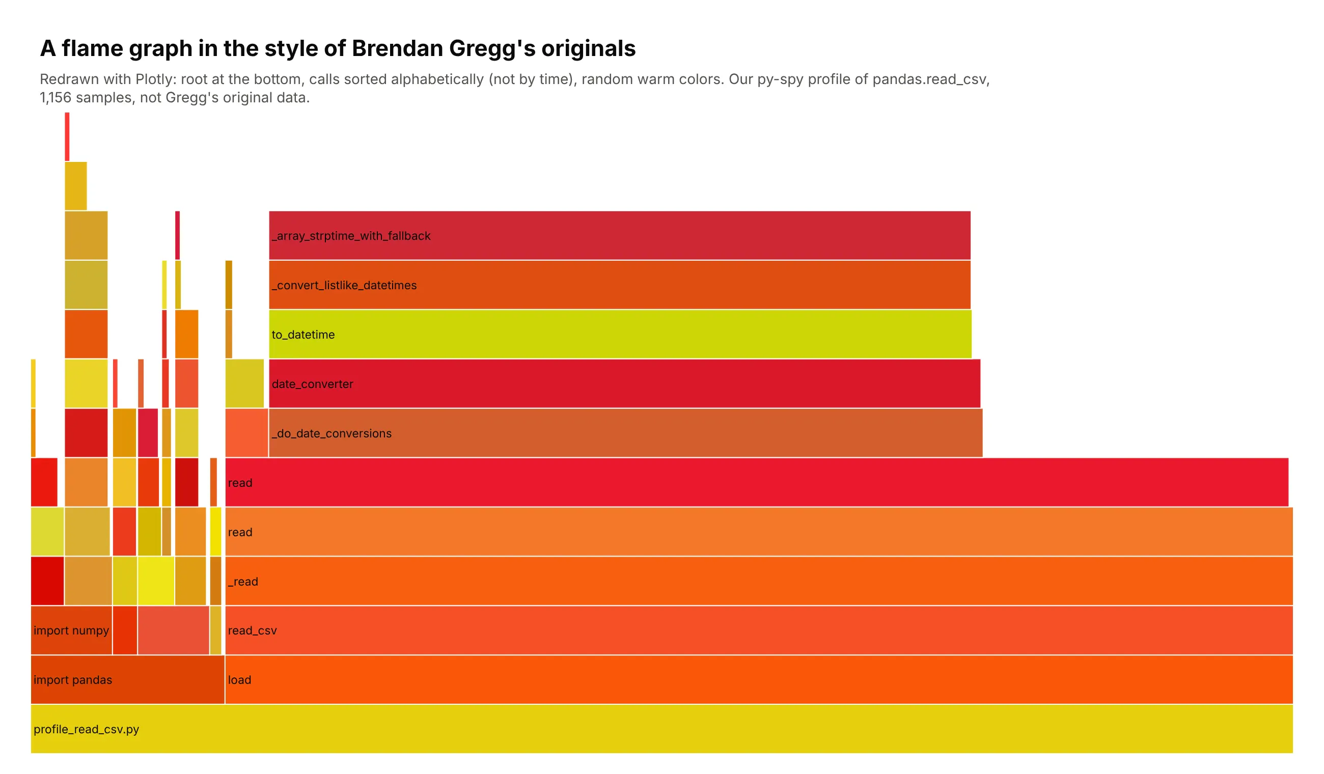
Flame graph of 1,156 CPU samples of pandas reading a 47.6 MB EIA-930 grid data CSV five times. Date conversion functions, in orange, take 67% of read_csv's time; the C parser's own time is 29%; import pandas is a narrower tower on the right

A CPU profile, drawn as a flame graph. Turned on its side with the root at the bottom, the chart shows that parsing two timestamp columns took 67% of the time pandas spent reading six months of hourly US grid data (47.6 MB, 264,934 rows). Data: EIA-930 Hourly Electric Grid Monitor, January to June 2025, profiled with py-spy.

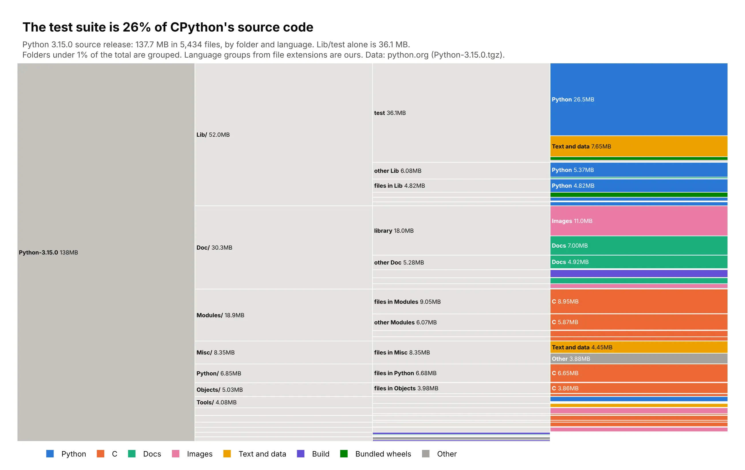
Horizontal icicle chart of the CPython 3.15.0 source release, 137.7 MB, by folder, subfolder and language. Lib/test is 36.1 MB, mostly Python in blue; Doc has 11.0 MB of images in pink; Modules is mostly C in orange

Files on a disk. The test suite is 36.1 MB of the 137.7 MB Python 3.15.0 source release, 26% of everything, and reads like a file explorer from left to right. Data: Python-3.15.0.tgz from python.org; language groups are ours.

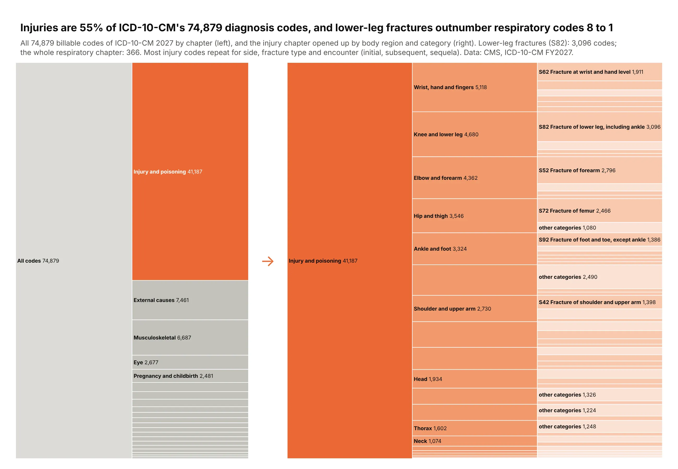
$Two icicle charts side by side: on the left, all 74,879 ICD-10-CM codes by chapter, with injury and poisoning (41,187) in orange; on the right, the injury chapter by body region and category, with lower-leg fractures (S82) at 3,096 codes$

A code set or classification. Injuries are 55% of the 74,879 billable ICD-10-CM diagnosis codes, and fractures of the lower leg alone have 3,096 codes, more than 8 times the whole respiratory chapter, because each repeats for side, fracture type and encounter. Data: CMS, ICD-10-CM FY2027 code files.

A short history

Joseph Kruskal and James Landwehr named the icicle plot in 1983, in The American Statistician, as a way to draw the results of hierarchical clustering. In 2011 Brendan Gregg drew CPU profiles the same way with the root at the bottom, sorted each level alphabetically so that identical call stacks merge, and gave the bars random warm colors, which is where the name flame graph comes from (Communications of the ACM, 2016). This is the profile above redrawn with Plotly in his original style:

Alternatives to an icicle chart

Here's the same refining capacity, by region and state, drawn six ways. Some are better for the question, some worse, some just different:

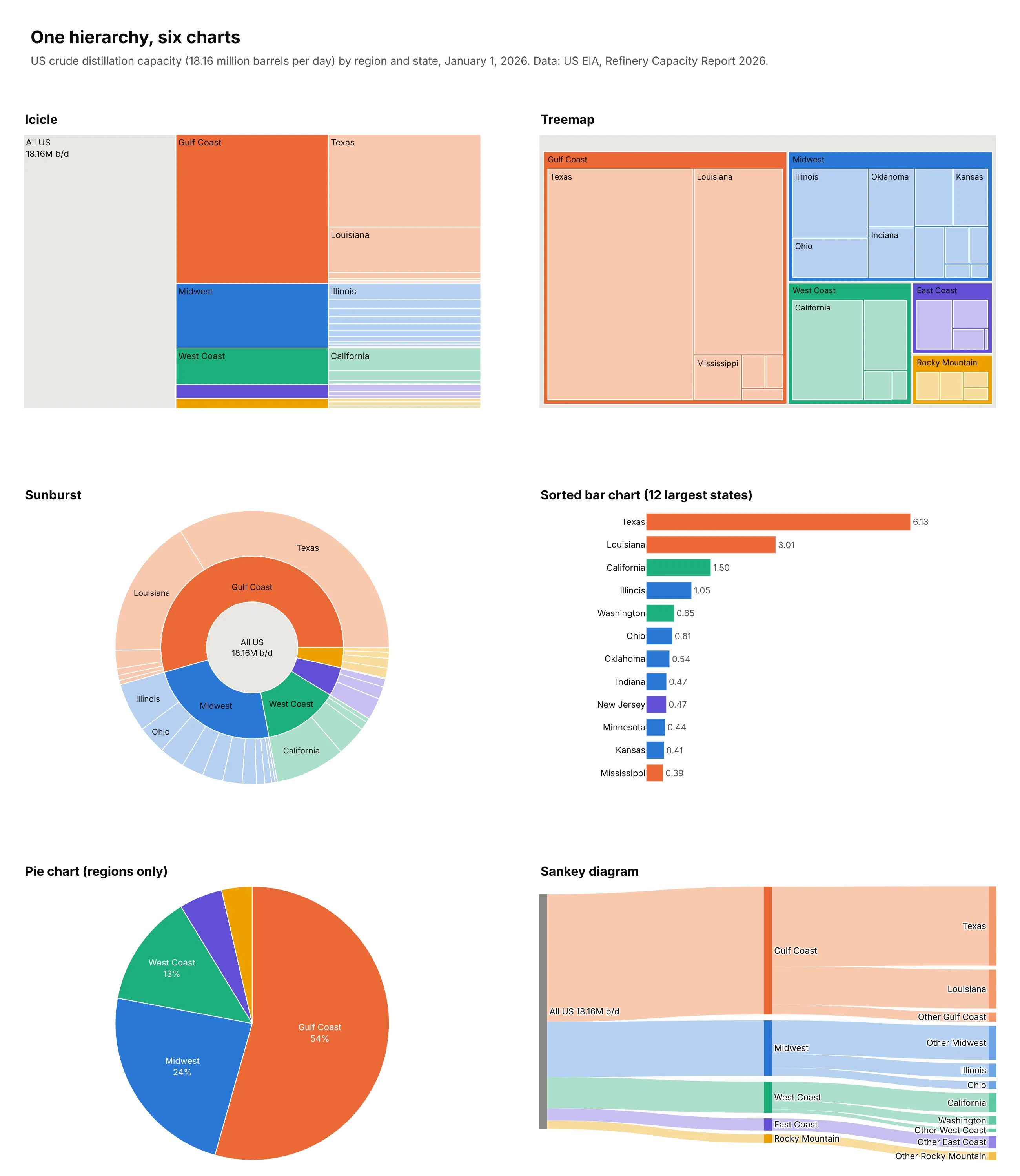
The same 18.16 million barrels per day of US refining capacity drawn six ways: an icicle chart, a treemap, a sunburst, a sorted bar chart of the 12 largest states led by Texas at 6.13, a pie chart of the five regions with the Gulf Coast at 54%, and a Sankey diagram flowing from the US total to regions to states

Sorted bar chart (better for one level). People judge lengths on a shared baseline more accurately than anything else, as Cleveland and McGill (1984) measured, and in an icicle chart only siblings share an edge. Use bars when one level answers the question. You lose the path from the total to each item.
Treemap (different). Nests each level inside its parent, so it fits the most leaves on one screen, but the levels are harder to follow. See our treemap guide.
Sunburst (different). The icicle bent into rings around the root, which is more compact but turns lengths into angles that are harder to compare and label. See our sunburst chart guide.
Pie chart (works too, for one level). Fine for the five regions sorted largest first, where the Gulf Coast is 54%, but it can't show the states inside them.
Sankey diagram (different). Draws the same split as flows from the total to regions to states, and also handles flows between stages that aren't a strict tree. See our Sankey diagram guide.

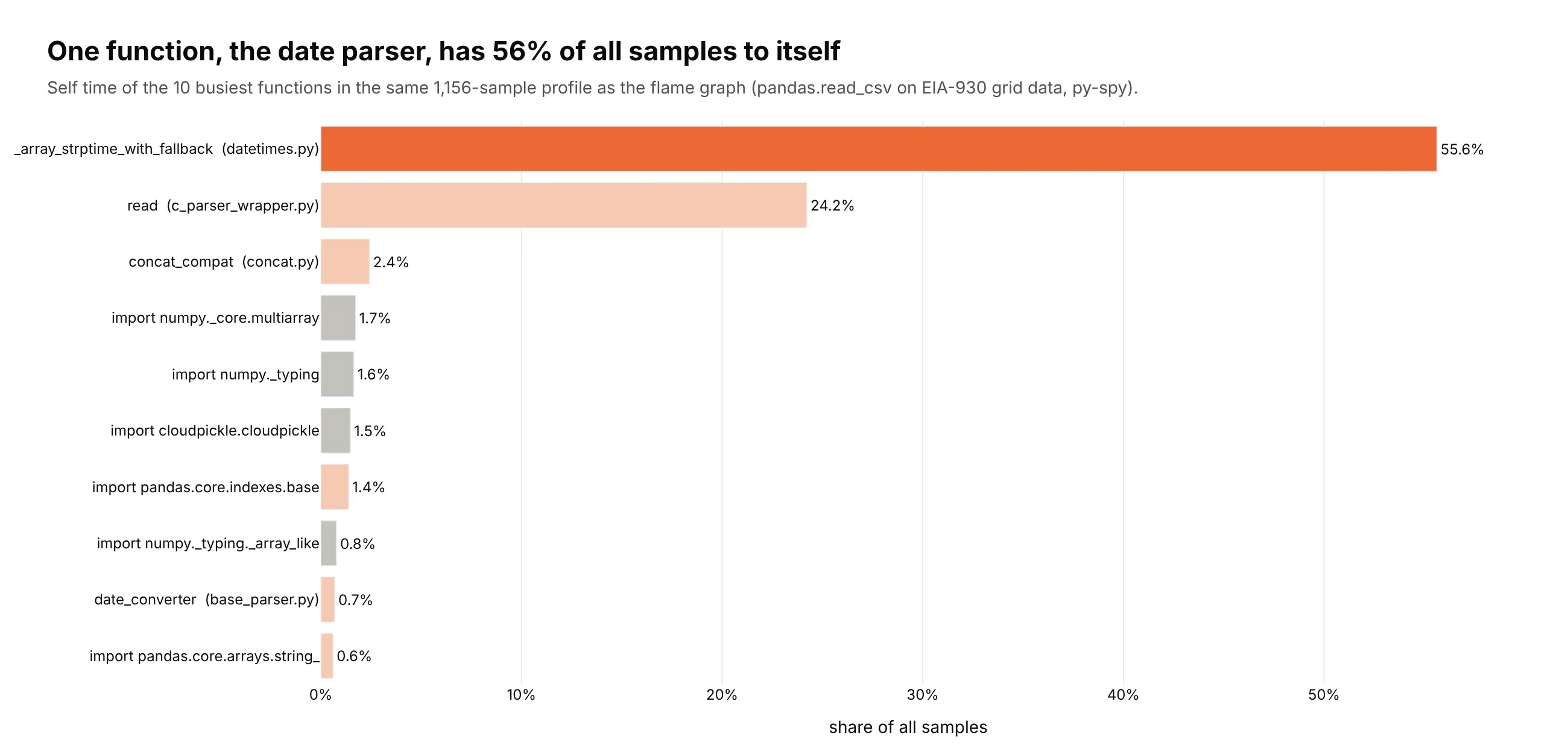
Here's where the bar chart wins. For the flame graph above, ranking functions by their own time (self time) shows at once that one function, _array_strptime_with_fallback, has 56% of all samples to itself, which you'd have to hunt for at the top of the tallest tower:

How to make an icicle chart

With AI

ChatGPT, Claude Code, GitHub Copilot, Cursor and other AI tools are excellent at writing Plotly code. Name Plotly in the prompt, describe the levels, the orientation and what color should mean, and list the checks you want:

Make a plotly flame graph from profile.txt (py-spy raw output: one call stack per line,
frames joined by ";", then a space and a sample count).

- go.Icicle with ids = the stack path, parents = the path minus the last frame,
  values = samples including callees, branchvalues="total".
- tiling orientation "v" with flip "y" (root at the bottom), leaf opacity 1.
- Drop frames under 0.4% of all samples. Label bars with the function name only;
  put the file in the hover with the share of samples.
- Color frames by library (pandas, numpy, standard library) in light tints, and the
  subtree I name in a strong orange.
- A title that states the share of time in that subtree.
- Assert that every node's value is at least the sum of its children.

With Plotly Studio

Plotly Studio is a desktop app where you point an AI at a dataset and it builds charts and a Dash app around your questions. Ask for an icicle chart the same way:

Show an icicle chart of refinery capacity by region, state and refinery, with one color per region, each bar labeled with its share of US capacity, and a dropdown to switch between operable and operating capacity.

Make an icicle chart in Python or JavaScript

This is the code AI tools write under the hood. In Python, Plotly Express builds the hierarchy from a flat table with one column per level:

import plotly.express as px

df = px.data.gapminder().query("year == 2007")
fig = px.icicle(df, path=[px.Constant("World"), "continent", "country"], values="pop")
fig.update_traces(root_color="#dcdbd6", leaf_opacity=1)
fig.show()

A flame graph starts from folded stacks, with one line per call stack, frames joined by ; and a sample count at the end. py-spy record -f raw -o profile.txt -- python your_script.py writes them, and this function draws them:

import plotly.graph_objects as go


def flame_graph(folded_path, min_share=0.004):
    """Flame graph from folded stacks ("main;load;read_csv 42" per line)."""
    nodes = {}
    for line in open(folded_path):
        stack, n = line.rsplit(" ", 1)
        frames = stack.split(";")
        for depth in range(1, len(frames) + 1):
            node_id = ";".join(frames[:depth])
            node = nodes.setdefault(node_id, {"parent": ";".join(frames[:depth - 1]),
                                              "label": frames[depth - 1].split(" (")[0], "value": 0})
            node["value"] += int(n)
    total = sum(v["value"] for k, v in nodes.items() if v["parent"] == "")
    keep = {k: v for k, v in nodes.items() if v["value"] >= min_share * total}
    return go.Figure(go.Icicle(
        ids=list(keep), parents=[v["parent"] for v in keep.values()],
        labels=[v["label"] for v in keep.values()], values=[v["value"] for v in keep.values()],
        branchvalues="total", tiling=dict(orientation="v", flip="y"),
        leaf=dict(opacity=1), hovertemplate="%{label}<br>%{percentRoot:.1%} of samples<extra></extra>",
    ))


flame_graph("profile.txt").show()

The empty space above a bar is the function's own time, and min_share drops frames too narrow to see. In a Dash app, clicking a bar zooms into it, and clickData["points"][0]["id"] tells your callback which node was clicked.

In JavaScript, plotly.js takes one entry per bar with its label, its parent and its value:

<div id="chart"></div>
<script src="https://cdn.plot.ly/plotly-4.1.1.min.js"></script>
<script>
  Plotly.newPlot("chart", [{
    type: "icicle",
    labels: ["All US refineries", "Gulf Coast", "Midwest", "Texas", "Louisiana", "Illinois", "Ohio"],
    parents: ["", "All US refineries", "All US refineries", "Gulf Coast", "Gulf Coast", "Midwest", "Midwest"],
    values: [18.16, 9.88, 4.28, 6.13, 3.01, 1.05, 0.61],
    branchvalues: "total",
    texttemplate: "<b>%{label}</b><br>%{value:.2f}M b/d"
  }]);
</script>

With branchvalues="total", a parent's value must be at least the sum of its children (the gaps here are the regions and states left out), or Plotly draws an empty chart without an error.

Share it

Every Plotly chart has a Share chart button (the cloud icon in its toolbar) that uploads it to Plotly Cloud and gives you a link. Only you can see it until you change its visibility.

For a live app, put the chart in a Dash app and publish it with the Plotly Cloud CLI. Coding agents can run these commands for you:

pip install "dash[cloud]"
plotly user login
plotly app publish

If your data has to stay in your own cloud or data center, publish to Dash Enterprise instead.

Dos and don'ts

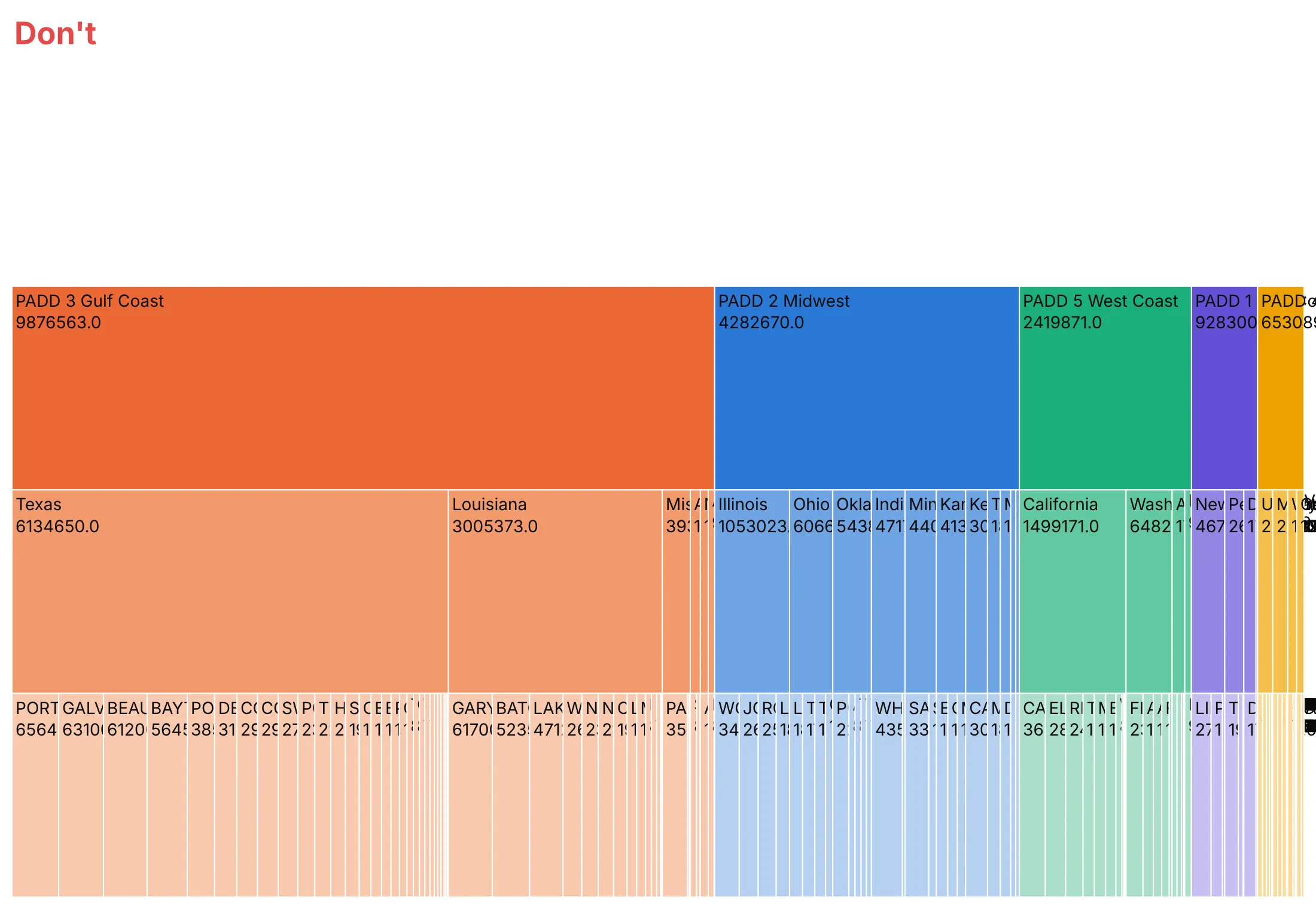
Plotly's defaults are made for exploring. For a published chart, most of the work is deciding what to leave out. Here is the same refinery data both ways.

Don't squeeze long names into a vertical layout, leave the root blank so the total is missing, print raw values straight from the data, or force a label onto every bar:

An icicle chart of the 124 US refineries in the same region colors as the next chart, but vertical, with a blank root row, raw values such as 9876563.0 and 656400.0, all-caps plant names, and labels forced onto every bar so the state and plant labels are cut off and overlap into unreadable text

Do go horizontal for long labels, label the root with the total, show formatted shares instead of raw numbers and hide the labels that don't fit. The colors are the same, one hue per region that gets lighter at each level:

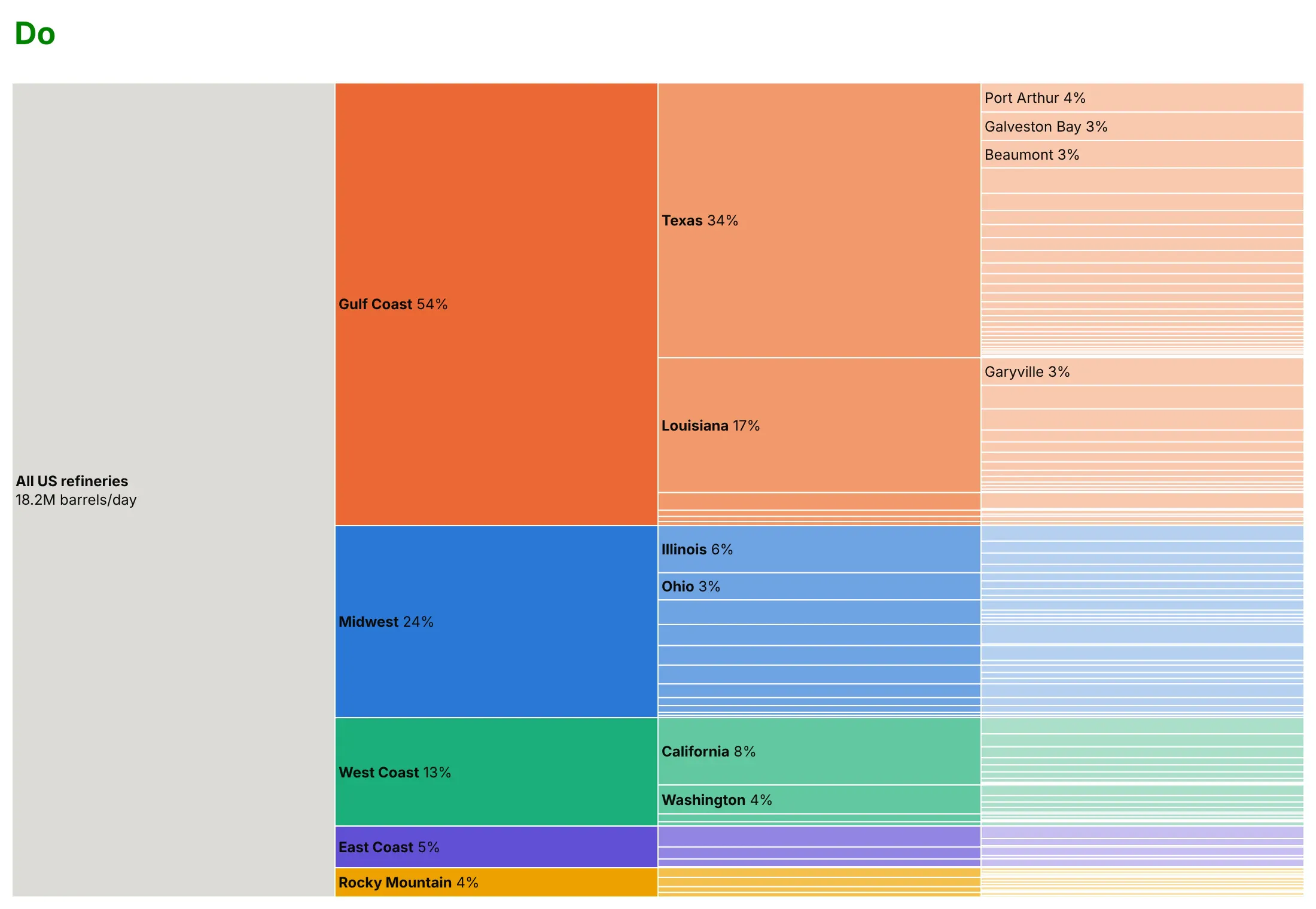
The same icicle chart designed on purpose: horizontal, a gray root labeled All US refineries 18.2M barrels/day, the Gulf Coast in orange at 54%, the Midwest in blue at 24%, the West Coast in green at 13%, states and plants in lighter shades of their region, and labels only on bars big enough to read, such as Texas 34% and Port Arthur 4%

Use color for one other thing

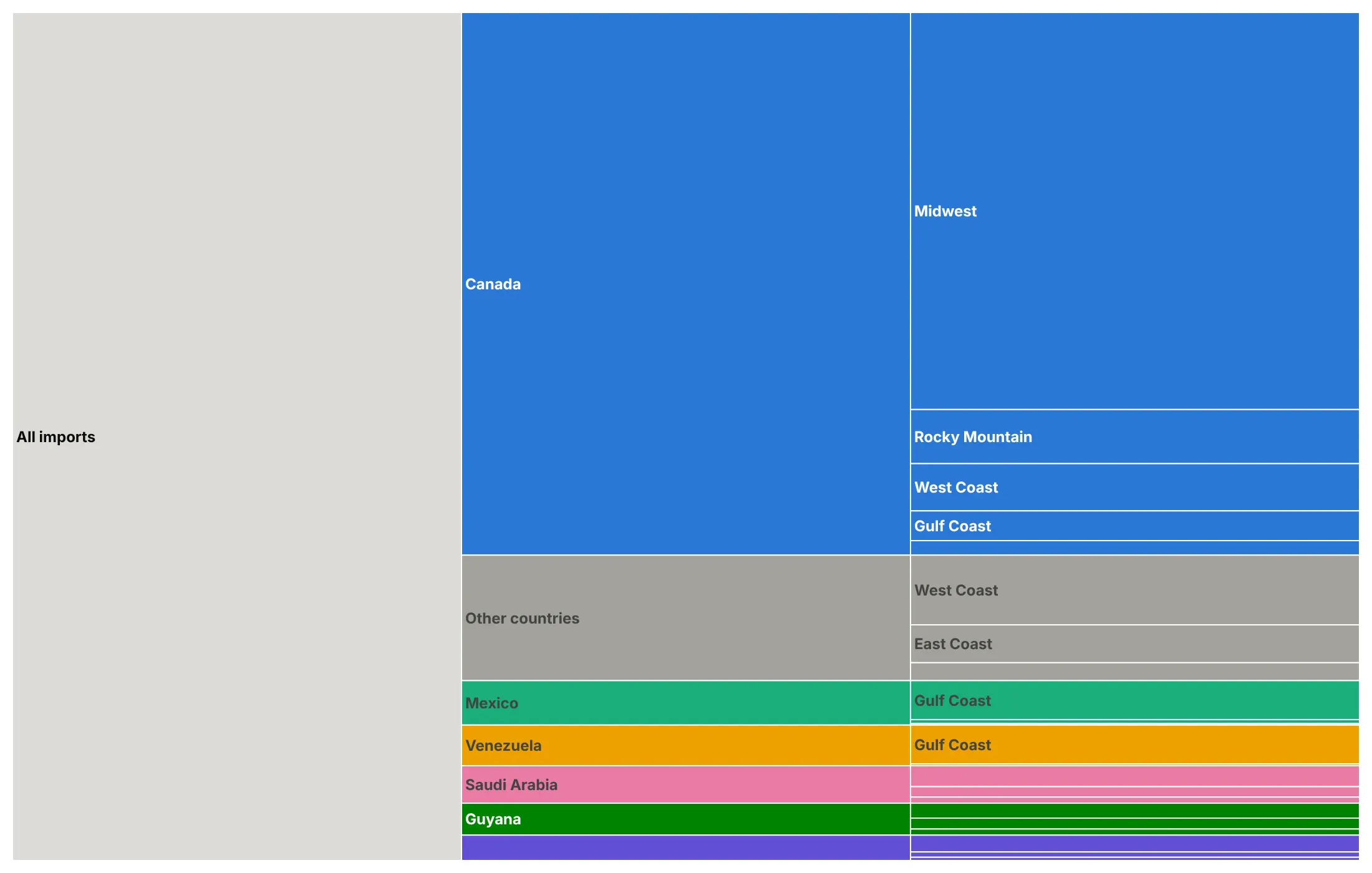
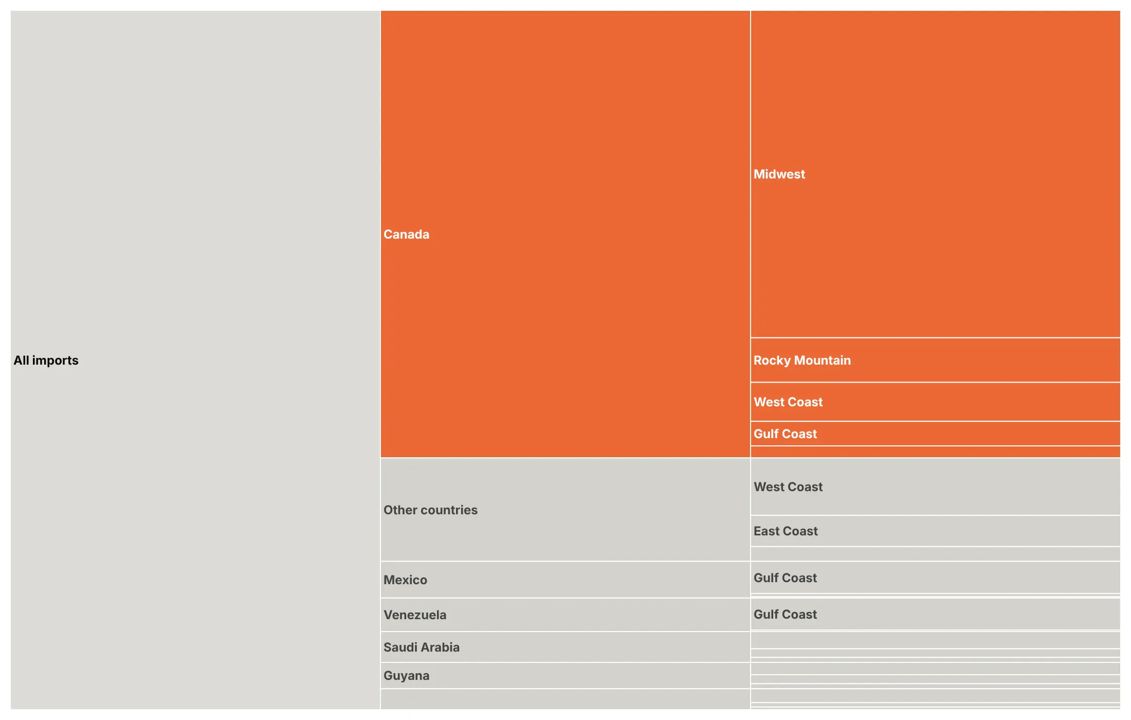
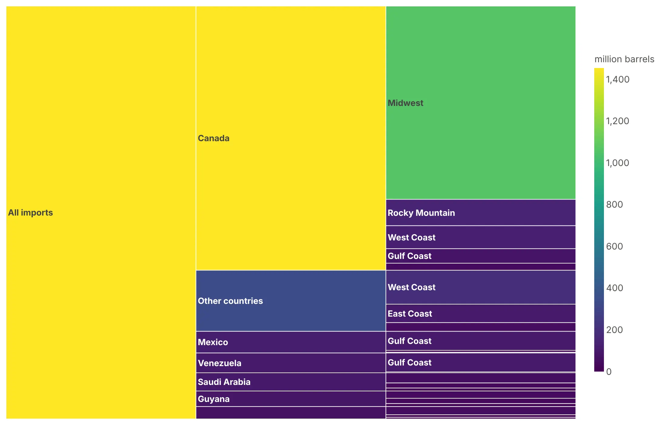
Bar length already shows size, so color is free to say something else. Here are four options on the same data, US crude oil imports from August 2025 to July 2026 by country of origin and destination region.

By group. One color per country, inherited by the regions it ships to, is a good default when the top level matters.

The crude imports icicle chart colored by country: Canada in blue, other countries in gray, Mexico in green, Venezuela in yellow, Saudi Arabia in pink, Guyana in dark green and Colombia in purple, with each country's destination regions in the same color

Highlight one story. Canada supplied 64% of the 2,272 million barrels, so it's the only color and everything else is gray.

The crude imports icicle chart with Canada and its destination regions in orange and every other bar in gray

By size (avoid). A color scale on the volume repeats what the bar heights already show, and the root takes the brightest color for no reason.

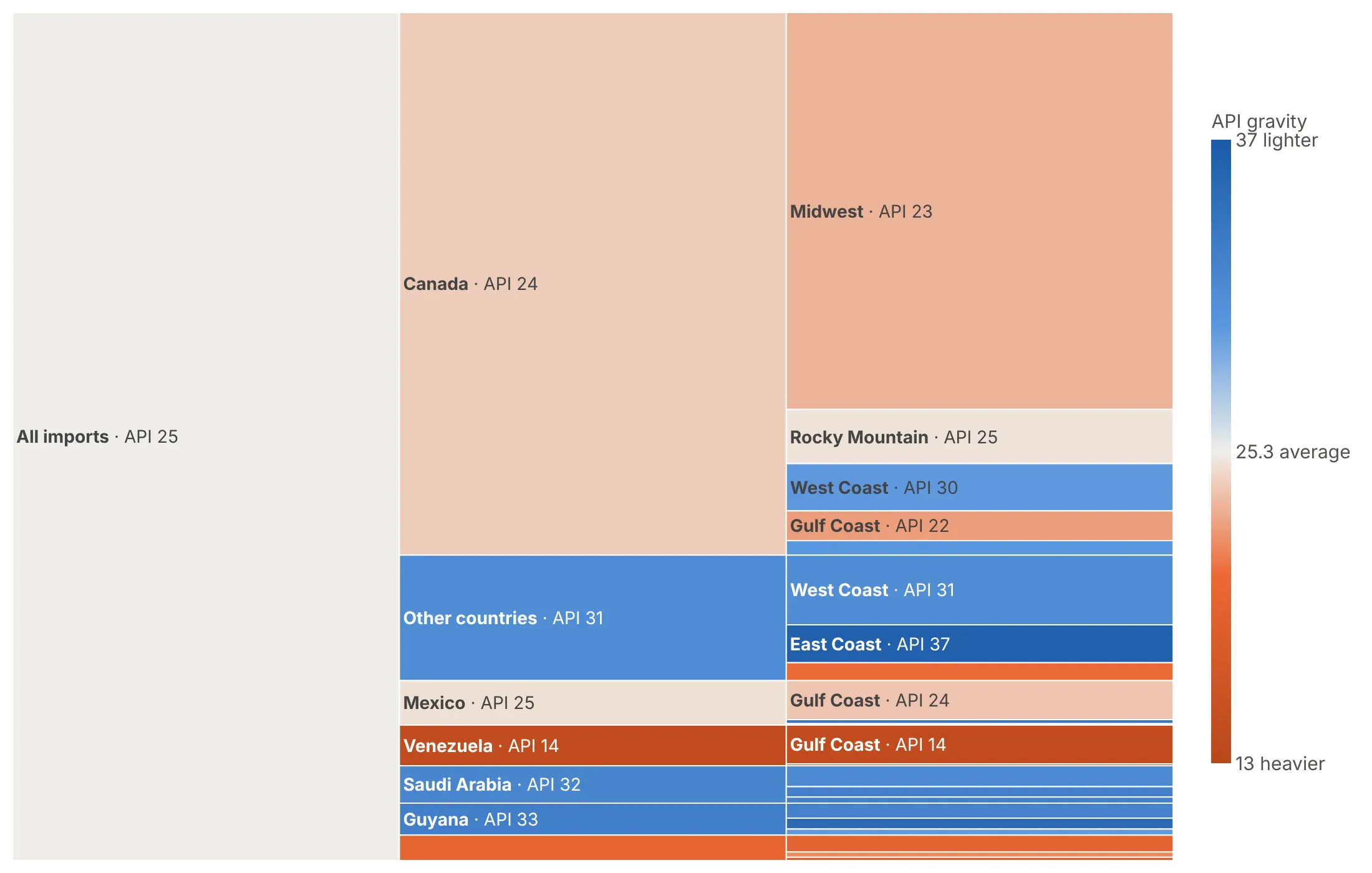
The crude imports icicle chart shaded on a Viridis scale by million barrels, so the root and Canada are bright yellow, the Midwest green and everything else nearly the same dark purple

By a second variable. Here it's API gravity, how light the crude is, on a diverging scale centered on the 25.3 average: Venezuela's crude, at API 14, is the darkest orange and the heaviest.

The crude imports icicle chart colored by volume-weighted API gravity from 13 (heavier, dark orange) through 25.3 (average, light gray) to 37 (lighter, dark blue). Canada is API 24, Venezuela 14 in dark orange, Saudi Arabia 32 and Guyana 33 in blue

Checklist

Write a title that states the takeaway, such as "Parsing two date columns took 67% of read_csv's time" instead of "CPU profile".
Go horizontal for long labels, and vertical for flame graphs and wide, shallow trees.
Label the root with the total, or start the drawing lower down with level.
Put values or shares on the bars with %{percentRoot} or %{percentParent}, and hide the rest with uniformtext=dict(minsize=10, mode="hide").
Fold the long tail into one "N more" bar per parent.

Don't

Color by size, because length already shows it.
Draw more than four levels in a static image, or force labels onto bars too thin to hold them.
Size bars by rates, averages or percentages, which don't add up.
Sort a timeline by size (use sort=False).

Options to customize

These are the go.Icicle (and px.icicle) options that matter most. The full list is in the Plotly icicle documentation.

path (px only): builds the tree from DataFrame columns, top level first.
ids, labels, parents: the tree, one row per bar. Use when labels repeat under different parents, such as function names.
values: the length of each bar.
branchvalues: total (a parent's value includes its children) or remainder (a node's own value, with its children added on top), which suits self time in a profile.
count: size by the number of "leaves" or "branches" when your records have no value column.
tiling.orientation: "h" (the default) puts levels in columns, "v" in rows.
tiling.flip: mirrors the layout with "x" or "y"; orientation="v", flip="y" makes a flame graph.
tiling.pad: the gap between bars, usually 0 for profiles.
marker.colors: one color per bar, for groups or a highlight.
marker.colorscale, cmid, cmin, cmax: map a number to color; cmid centers a diverging scale.
leaf.opacity: 0.7 by default; set it to 1 for exact colors.
texttemplate: bar text with %{label}, %{value}, %{percentRoot} and %{percentParent}.
uniformtext (layout): a minimum font size; mode="hide" drops text that won't fit.
maxdepth, level: how many levels to draw at once, and which node to start from.
pathbar.visible, root.color: a breadcrumb bar for zoomed views, and the root's color.
sort: set to False to keep your own order, for timelines and hand-ordered rows.
domain: place several icicle charts side by side.

More icicle chart examples

Nine more icicle charts built from real public data, each with its source, the technique that makes it work and a prompt to rebuild it.

1. What import plotly.express spends its time on

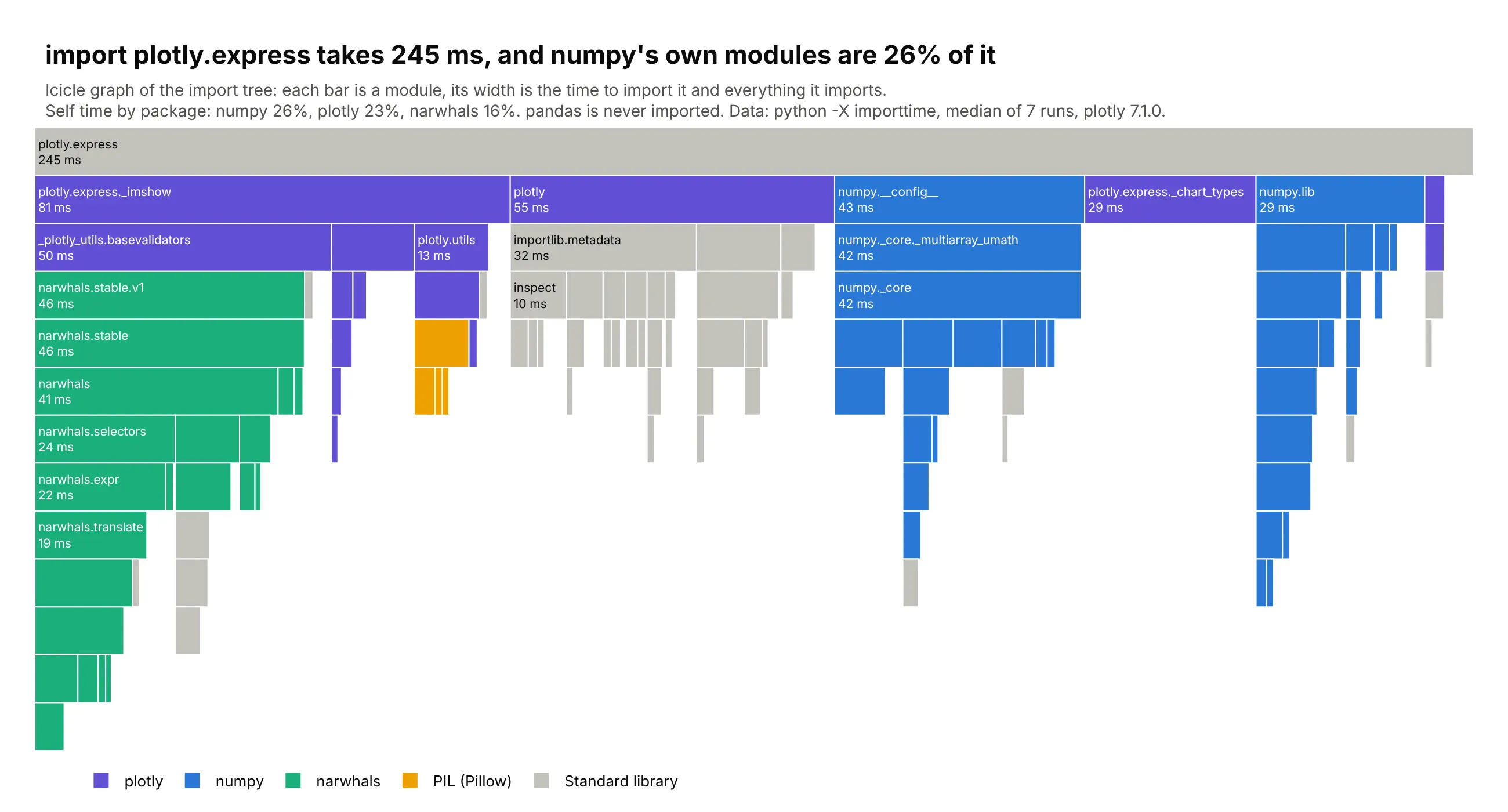
Icicle graph of the import tree of plotly.express, 245 ms in total, with the root on top. numpy modules in blue are 26% of the time, plotly in purple 23% and narwhals in green 16%

Python's -X importtime flag prints an import tree with each module's own time. import plotly.express took 245 ms (median of 7 runs), and numpy's own modules were 26% of it, plotly's 23% and narwhals' 16%, while pandas is never imported. Data: python -X importtime, plotly 7.1.0, Python 3.13.

Tip: pass each node's own time as values with branchvalues="remainder", and plotly adds the children for you.

Get the data from CPython's import profiler: run
python -X importtime -c "import plotly.express" 2> imports.txt
seven times and keep the median run. Parse the tree from the indentation into a table
(columns: id = import path, module, parent, self_us, cumulative_us, package).

Build a plotly icicle chart with the root on top (tiling orientation "v", no flip).
- values = self_us with branchvalues="remainder", so widths include imported modules.
- Drop modules under 0.4% of the total, adding their time to their parent.
- One color per top-level package (plotly, numpy, narwhals, PIL), standard library gray,
  legend from invisible scatter traces.
- Label bars "module<br>N ms"; title with the total and the biggest package's share.

2. The structure of MDN Web Docs

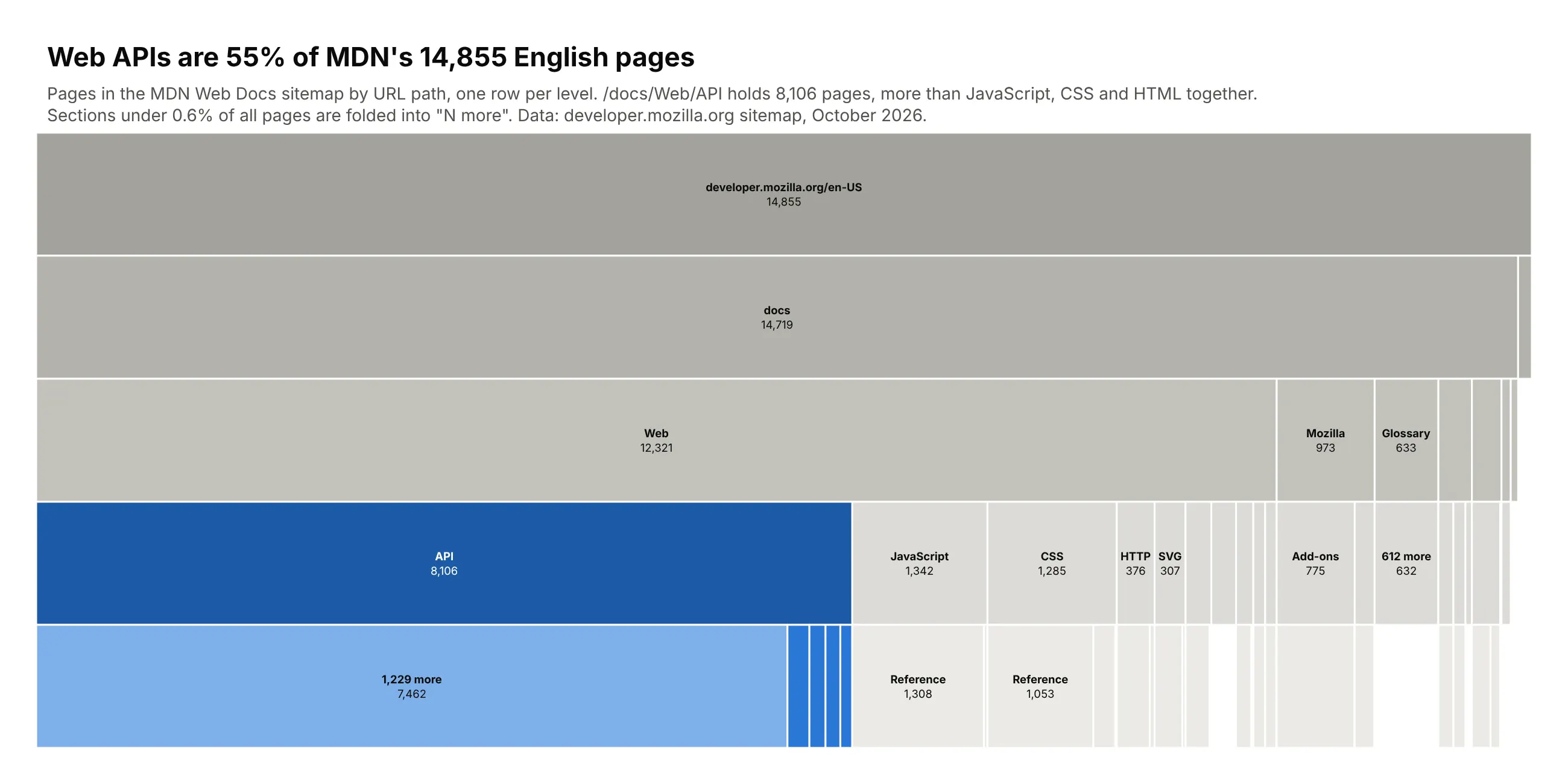
Vertical icicle chart of MDN Web Docs' 14,855 English pages by URL path. /docs/Web/API, in blue, has 8,106 pages; JavaScript has 1,342 and CSS 1,285

A sitemap is a tree of URL paths, and counting pages per path shows where a site's content lives. MDN has 14,855 English pages, and 55% of them sit under /docs/Web/API, more than JavaScript, CSS and HTML together. Data: developer.mozilla.org English sitemap, October 2026.

Tip: tiling.orientation="v" draws a classic top-down site map, which suits a wide, shallow tree.

Get the data from MDN's English sitemap (developer.mozilla.org/sitemaps/en-us/sitemap.xml.gz).
Split every URL after /en-US/ into path segments and count pages
(columns: l1, l2, l3, l4, pages).

Build a plotly icicle chart with tiling orientation "v" (home page on top, one row per level).
- Fold children under 0.6% of all pages into one "N more" bar per parent.
- Color /docs/Web/API in blue and everything else in grays, darker for higher levels.
- Center the label and page count in each bar; title with the API share.

3. Where US crude oil imports come from, and how heavy they are

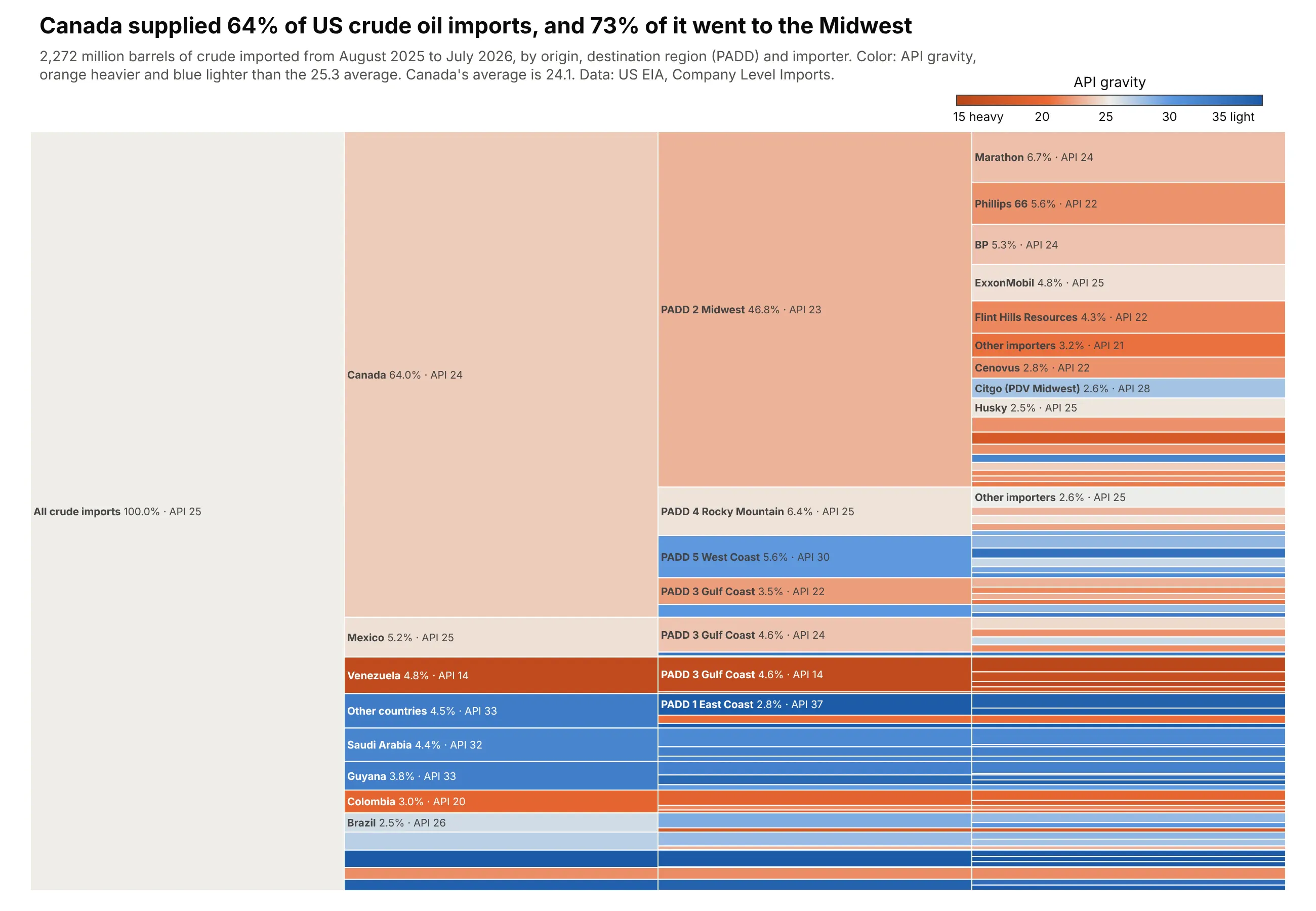
Horizontal icicle chart of 2,272 million barrels of US crude imports by origin country, destination region and importer, colored by API gravity. Canada is 64% and mostly goes to the Midwest; Venezuela, at API 14, is the darkest orange

The US imported 2,272 million barrels of crude in the 12 months to July 2026. Canada supplied 64%, and 73% of Canada's oil went to Midwest refineries. Color shows API gravity, and Venezuela's crude, at 14, is the heaviest against a 25.3 average. Data: EIA Company Level Imports, August 2025 to July 2026.

Tip: compute the color of every parent as the volume-weighted average of its children, not a plain average.

Get the data from EIA's Company Level Imports (eia.gov/petroleum/imports/companylevel),
the monthly import.xlsx files for August 2025 to July 2026, crude oil only
(columns: country, company, padd, kbbl, api_gravity and sulfur_pct volume-weighted).

Build a horizontal plotly icicle chart: all imports -> country -> destination PADD -> importer.
- Fold countries under 1.5% and importers under 0.6% into "other".
- Color every node by volume-weighted API gravity on an orange-gray-blue scale with cmid at the
  overall average, cmin/cmax 12 either side; horizontal colorbar.
- Label bars "name 64.0% · API 24". Title with Canada's share and where it goes.

4. Who holds the US public debt

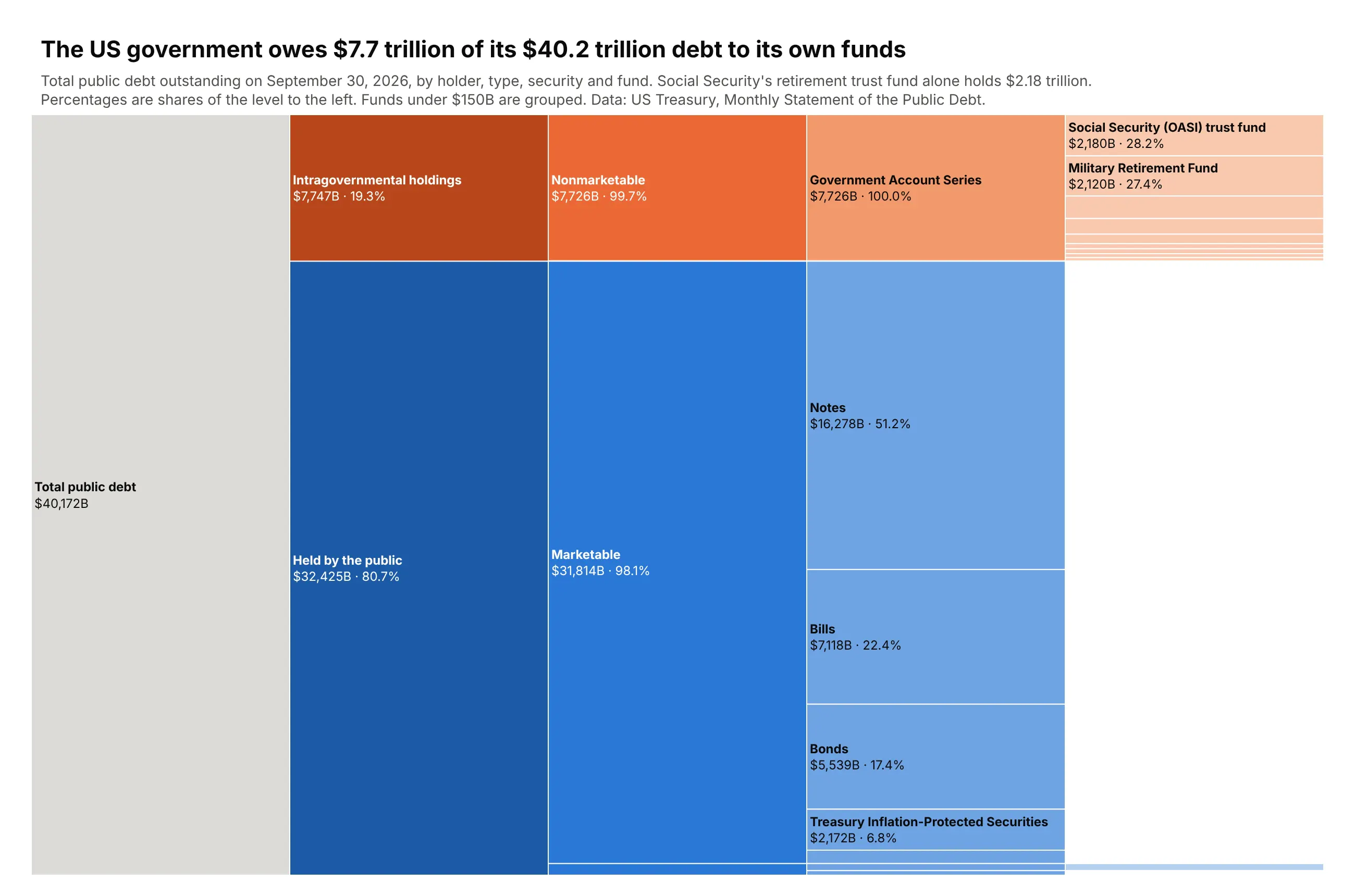
Horizontal icicle chart of the $40.2 trillion US public debt by holder, type, security and fund. Intragovernmental holdings of $7.7 trillion are on top in orange, led by the Social Security trust fund ($2.18 trillion) and the Military Retirement Fund ($2.12 trillion); the $32.4 trillion held by the public is in blue, half of it in notes

Of the $40.2 trillion of US public debt on September 30, 2026, the government owed $7.7 trillion to its own funds. Social Security's retirement trust fund alone held $2.18 trillion. Data: US Treasury, Monthly Statement of the Public Debt, September 2026.

Tip: sort=False with rows ordered by hand puts the branch that tells the story on top, even when it isn't the biggest.

Get the data from the US Treasury's Monthly Statement of the Public Debt for September 30, 2026
(Fiscal Data API tables mspd_table_1 and mspd_table_3_nonmarket)
(columns: holder, kind, security, account, amount_bn).

Build a horizontal plotly icicle chart: total -> holder -> marketable/nonmarketable -> security -> fund.
- Intragovernmental holdings in orange shades, held by the public in blue shades, darker higher up.
- sort=False, intragovernmental rows first, then by size.
- Labels "<b>name</b><br>$7,726B · 99.7%" with %{percentParent}; group funds under $150B.
- Assert the leaves add up to the total. Title with the intragovernmental total.

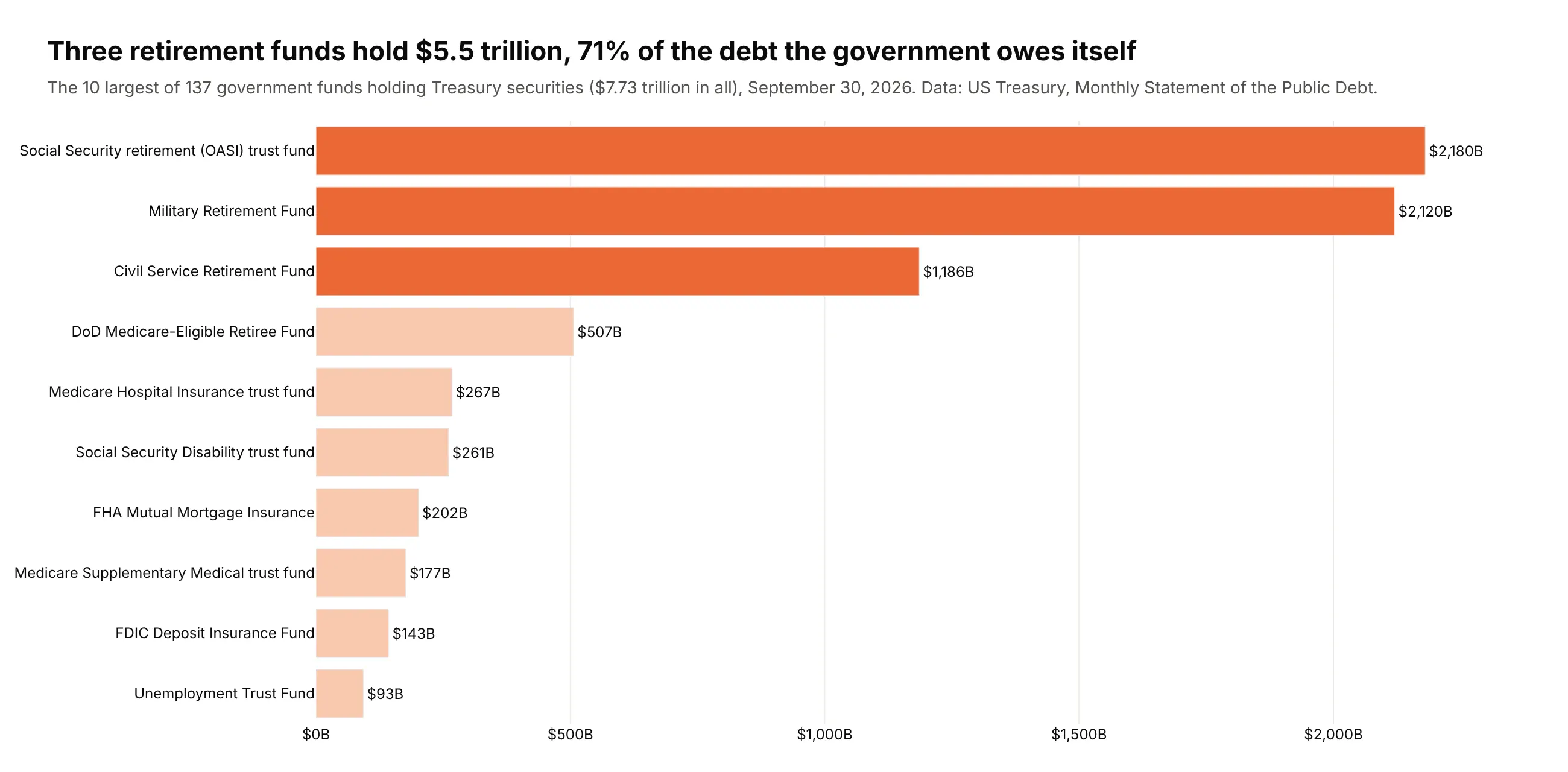
Another way to see it: a bar chart of the 10 largest funds shows that three retirement funds hold $5.5 trillion, 71% of the debt the government owes itself.

Bar chart of the 10 government funds holding the most Treasury securities: Social Security retirement $2,180B, Military Retirement $2,120B, Civil Service Retirement $1,186B, down to the Unemployment Trust Fund at $93B

5. US bank failures since 1934

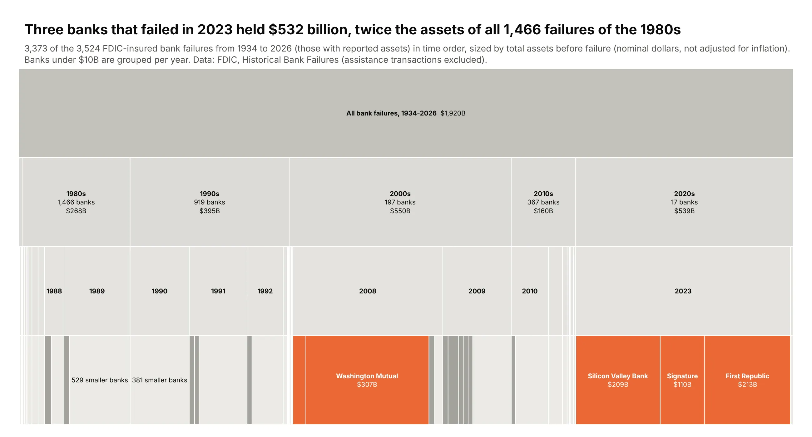
Vertical icicle chart of US bank failures from 1934 to 2026 by decade, year and bank, sized by assets. The 1980s are thousands of slivers worth $268 billion, while Washington Mutual ($307 billion) in 2008 and Silicon Valley Bank, Signature and First Republic ($532 billion together) in 2023 are wide orange bars

Sized by assets, the three banks that failed in spring 2023 held $532 billion, twice the $268 billion held by all 1,466 banks that failed in the 1980s (in nominal dollars). Counting failures would tell the opposite story. Data: FDIC Historical Bank Failures, failures only.

Tip: with sort=False and rows sorted by date, a vertical icicle becomes a timeline that reads left to right.

Get the data from the FDIC's Historical Bank Failures data (api.fdic.gov/banks/failures)
(columns: date, year, name, city, type, fund, assets_bn, deposits_bn, cost_bn, cert).

Build a plotly icicle chart with tiling orientation "v": all failures -> decade -> year -> bank,
sized by assets, failures only, sort=False with rows in date order.
- Fold banks under $10B into "N smaller banks" per year.
- Banks over $30B orange with name and assets, everything else gray.
- Note nominal dollars in the subtitle. Title comparing 2023 with the 1980s.

6. FDA drug approvals in 2025

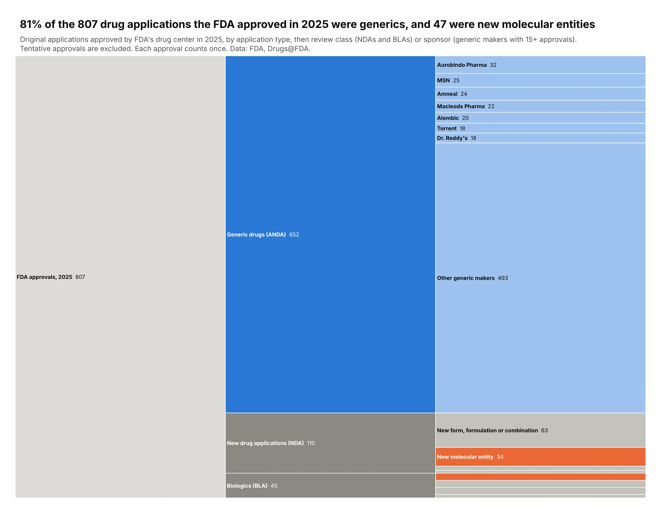
Horizontal icicle chart of 807 original drug applications FDA approved in 2025. Generic drugs (ANDA) are 652 in blue, led by Aurobindo, MSN and Amneal; new drug applications 110 and biologics 45 in gray, with 47 new molecular entities in orange

FDA's drug center approved 807 original applications in 2025, and 81% of them were generics. Only 47 were new molecular entities, 34 drugs and 13 biologics. Data: FDA Drugs@FDA data files; tentative approvals excluded.

Tip: count="leaves" sizes every node by its number of records, so you pass no values, and maxdepth=3 hides the 807 leaf rows in the static image.

Get the data from FDA's Drugs@FDA data files (fda.gov/media/89850/download), original
applications approved in 2025 (columns: appl_no, appl_type, submission_class, sponsor, drug, date).

Build a horizontal plotly icicle chart: all approvals -> application type -> review class
(for NDAs and BLAs) or sponsor (for generics, sponsors with 15+ approvals, the rest grouped).
- One leaf per approved application; count="leaves", maxdepth=3, sort=False.
- New molecular entities orange, generics blue, everything else gray.
- Pass the counts as customdata for the labels. Title with the generic share and the NME count.

7. Software in FDA 510(k) radiology clearances

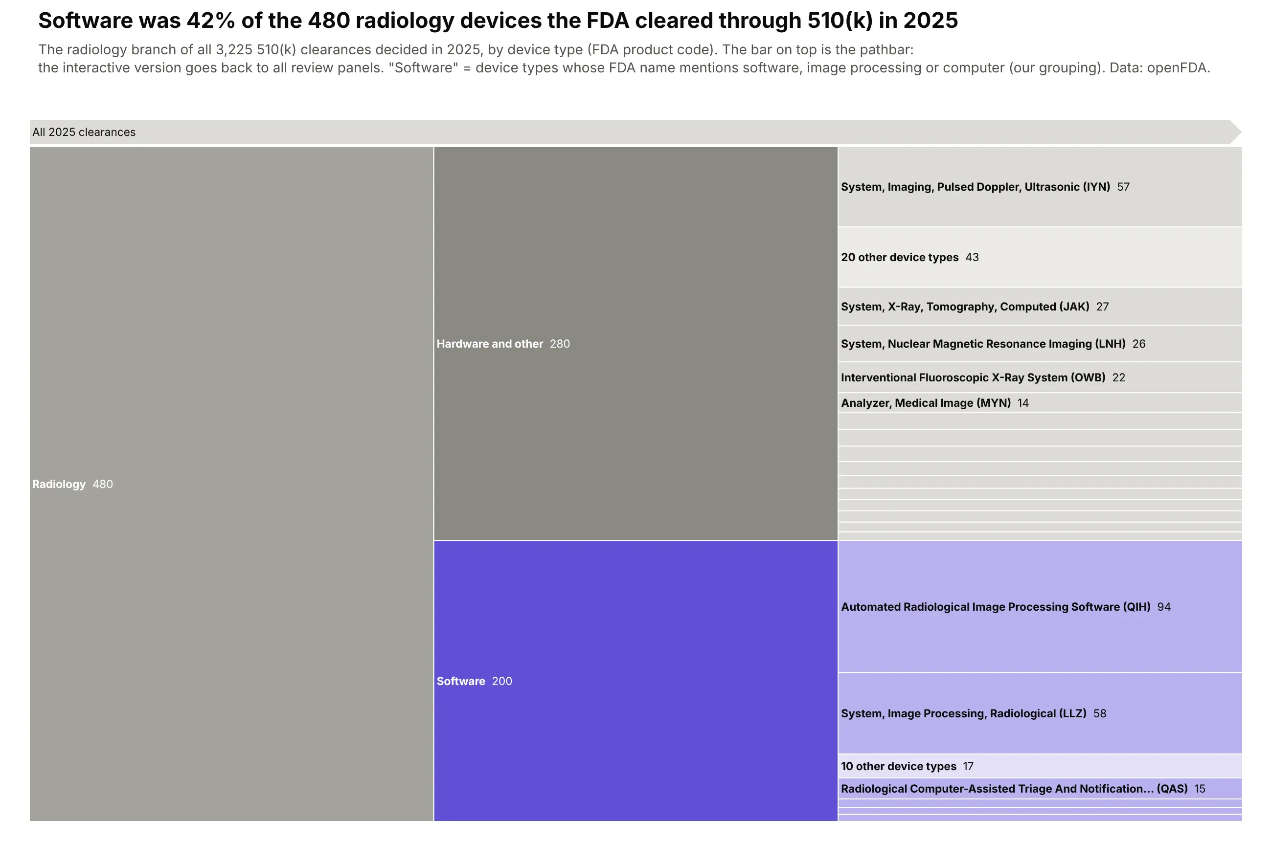
Horizontal icicle chart of the 480 radiology devices cleared through 510(k) in 2025, with a pathbar on top reading All 2025 clearances. Software device types in purple are 200 of them, led by automated radiological image processing software (94)

The FDA decided 3,225 510(k) clearances in 2025, and radiology was the largest panel with 480. Software device types, such as automated radiological image processing (94), made up 200 of them, 42%. Data: openFDA device 510(k) endpoint; the software grouping is ours.

Tip: level="All 2025 clearances/Radiology" starts the drawing at one branch, and pathbar=dict(visible=True) keeps the way back to the whole tree.

Get the data from openFDA's device 510(k) endpoint (api.fda.gov/device/510k.json),
decisions dated 2025 (columns: k_number, decision_date, panel, product_code, device_name, country).

Build a horizontal plotly icicle chart: all clearances -> review panel -> software vs hardware
(device names mentioning software, image processing or computer) -> product code.
- level set to the Radiology node and a visible pathbar on top.
- Software purple, hardware gray; product codes under 5 clearances grouped as "N other device types".
- Title with the software share of radiology.

8. The geologic time scale, to scale

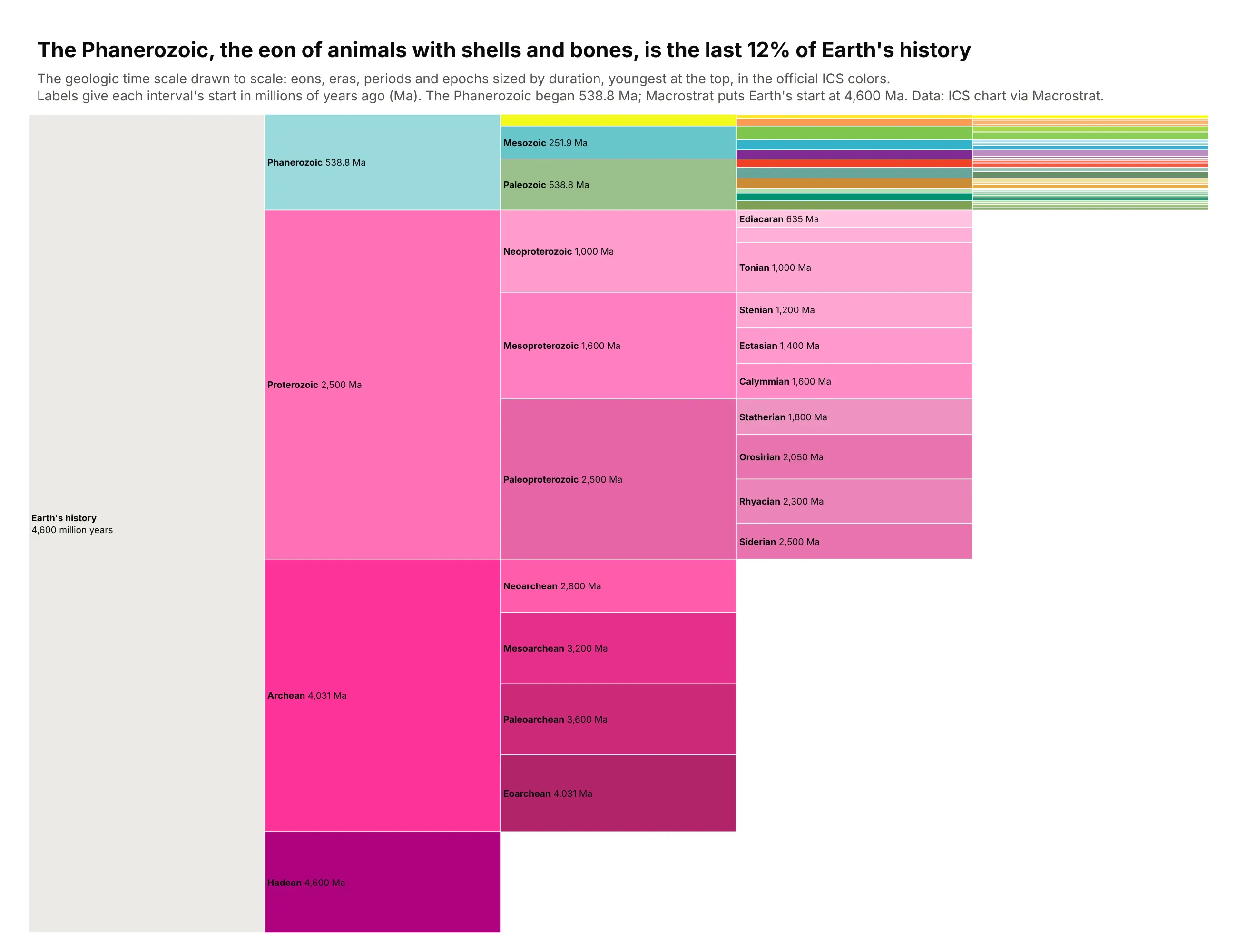
Horizontal icicle chart of the geologic time scale sized by duration, in ICS colors, youngest at the top. The Phanerozoic is the top 12% of the 4,600 million years; the Proterozoic and Archean fill most of the chart

The official chart of geologic time draws every interval at the same height. Drawn to scale, the Phanerozoic, the eon of animals with shells and bones, is only the last 12% of Earth's history. Data: ICS International Chronostratigraphic Chart via the Macrostrat API.

Tip: sort=False keeps time in order, and marker.colors takes the official ICS color of every interval.

Get the data from the Macrostrat API's international intervals
(macrostrat.org/api/v2/defs/intervals?timescale_id=11, plus the Hadean)
(columns: name, rank, parent, top_ma, base_ma, duration_my, color).

Build a horizontal plotly icicle chart: Earth's history -> eon -> era -> period -> epoch,
sized by duration, sort=False with the youngest interval at the top.
- marker.colors = the ICS color of each interval; root light gray.
- Label "<b>name</b> 538.8 Ma" with the start age; hide labels that don't fit.
- Title with the Phanerozoic's share.

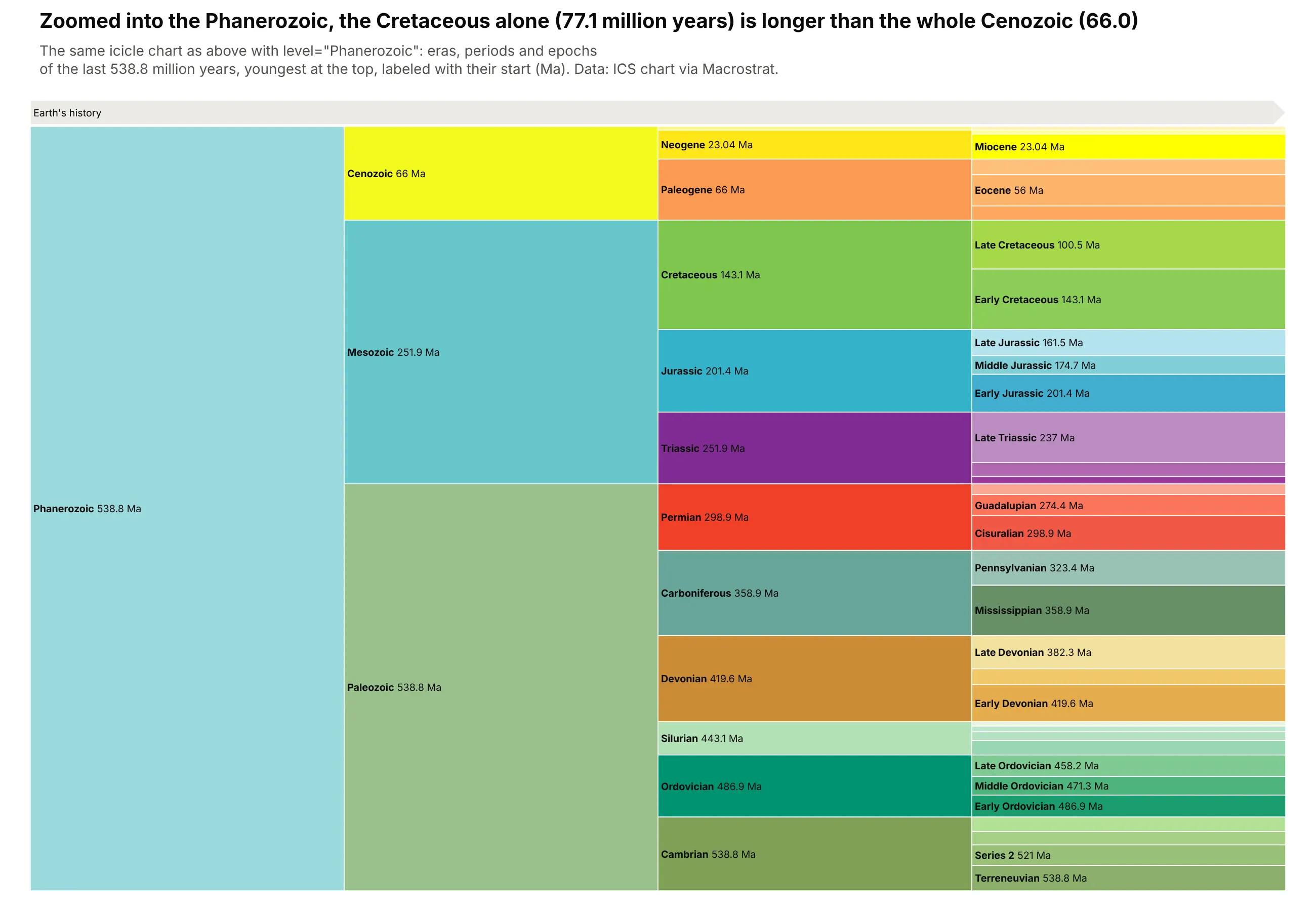
Another way to see it: the same chart with level="Phanerozoic" gives the last 538.8 million years the full height. The Cretaceous alone (77.1 million years) is longer than the whole Cenozoic (66.0).

The geologic time scale icicle chart zoomed into the Phanerozoic with a pathbar back to Earth's history: Cenozoic, Mesozoic and Paleozoic eras with their periods and epochs, in ICS colors

9. Every character in Unicode

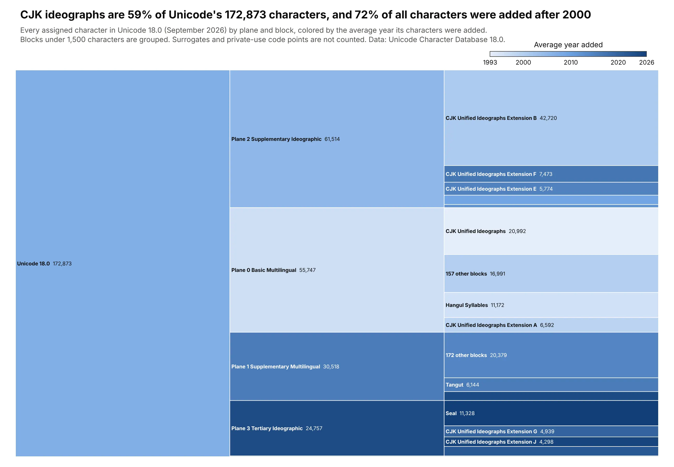
Horizontal icicle chart of Unicode 18.0's 172,873 characters by plane and block, colored by the average year added. CJK Unified Ideographs Extension B (42,720) is the largest block; plane 3 and the new Seal block are the darkest blue

Unicode 18.0 assigns 172,873 characters, and 59% are CJK ideographs. Color shows when they arrived, and 72% of all characters were added after 2000. Data: Unicode Character Database 18.0 and unicode.org release dates.

Tip: a sequential color scale for a second measure (here the average year added) adds a time dimension that the lengths can't show.

Get the data from the Unicode Character Database (unicode.org/Public/UCD/latest/ucd:
UnicodeData.txt, Blocks.txt, DerivedAge.txt) and the release years on unicode.org
(columns: plane, block, category, version, year, characters).

Build a horizontal plotly icicle chart: Unicode 18.0 -> plane -> block, sized by characters.
- Fold blocks under 1,500 characters into "N other blocks" per plane.
- Color every node by its character-weighted average year on a light-to-dark blue scale
  (1993-2026) with a colorbar.
- Title with the CJK share and the share added after 2000.