Chris Parmer

October 24, 2026

Parallel Coordinates Plots - A Complete Guide

TL;DR

A parallel coordinates plot draws each variable as a vertical axis and each record as a line that crosses every axis at its value, so hundreds or thousands of records across 4 to 10 measures fit in one chart.
Parallel coordinates plots are also known as parallel coordinate plots or PCPs, and are similar to scatter plot matrices and radar charts.
Its strength is brushing: drag a range on one or more axes and only the lines inside every range stay in color. In Plotly that's constraintrange, which also shows the brushed state in a static image.
Only neighboring axes can be compared, so the axis order decides what readers see. Use a scatterplot matrix for exact pairwise relationships and a parallel categories diagram for categorical columns.
Any coding agent can make one with Plotly in a minute. In Python it's px.parallel_coordinates(df, color=...), or go.Parcoords for fixed ranges and brushes.

What is a parallel coordinates plot?

Parallel coordinates plots look like this:

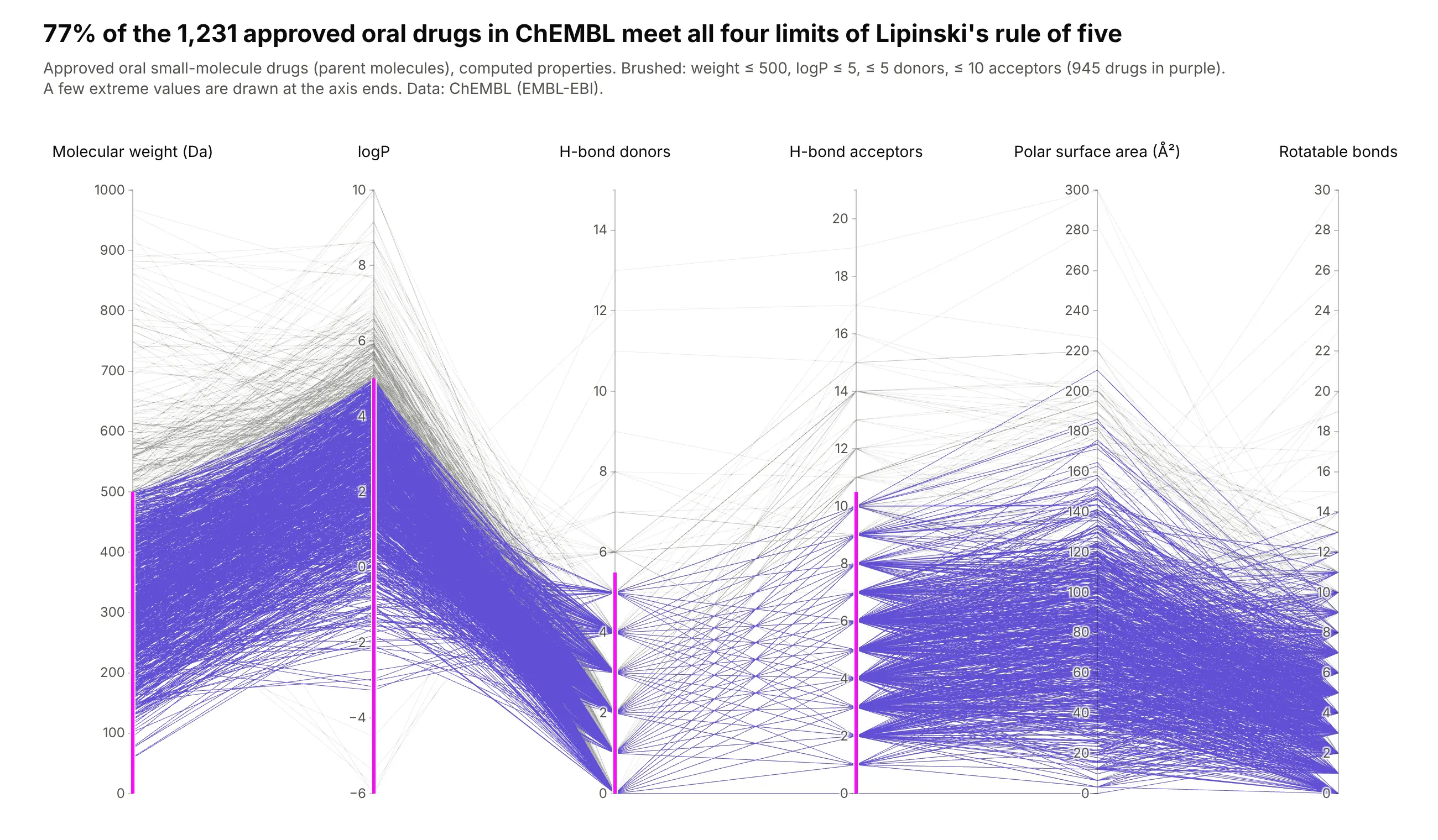
Parallel coordinates of 1,231 approved oral drugs across molecular weight, logP, H-bond donors, H-bond acceptors, polar surface area and rotatable bonds, with four brushes for Lipinski's limits: 945 purple lines pass

Data: ChEMBL (EMBL-EBI), approved oral small-molecule drugs.

How do you read a parallel coordinates plot? In the example above, notice these things:

Each line is one approved oral drug, and each of the six vertical axes is one of its computed properties, from molecular weight on the left to rotatable bonds on the right. The point where a line crosses an axis is that drug's value for that property.
Every axis has its own scale, so the same height means a different value on each axis. A line that climbs from logP to H-bond donors only reflects the change of scale, so compare positions on one axis at a time.
The pink bars are brushes, one for each of the four limits in Lipinski's rule of five (Lipinski et al., 1997). The 945 drugs whose lines pass through all four bars stay purple, and the rest turn gray.
The gray lines show which limit a drug breaks. Most of them leave the purple band at the top of the molecular weight or logP axis, while far fewer rise above the bars for H-bond donors and acceptors.
The zigzags around the H-bond donors and acceptors axes come from whole-number counts, where hundreds of drugs share the same value. Read those crossings as ties instead of a pattern, and hover or brush to pick out single drugs.

It's often used for charts like these:

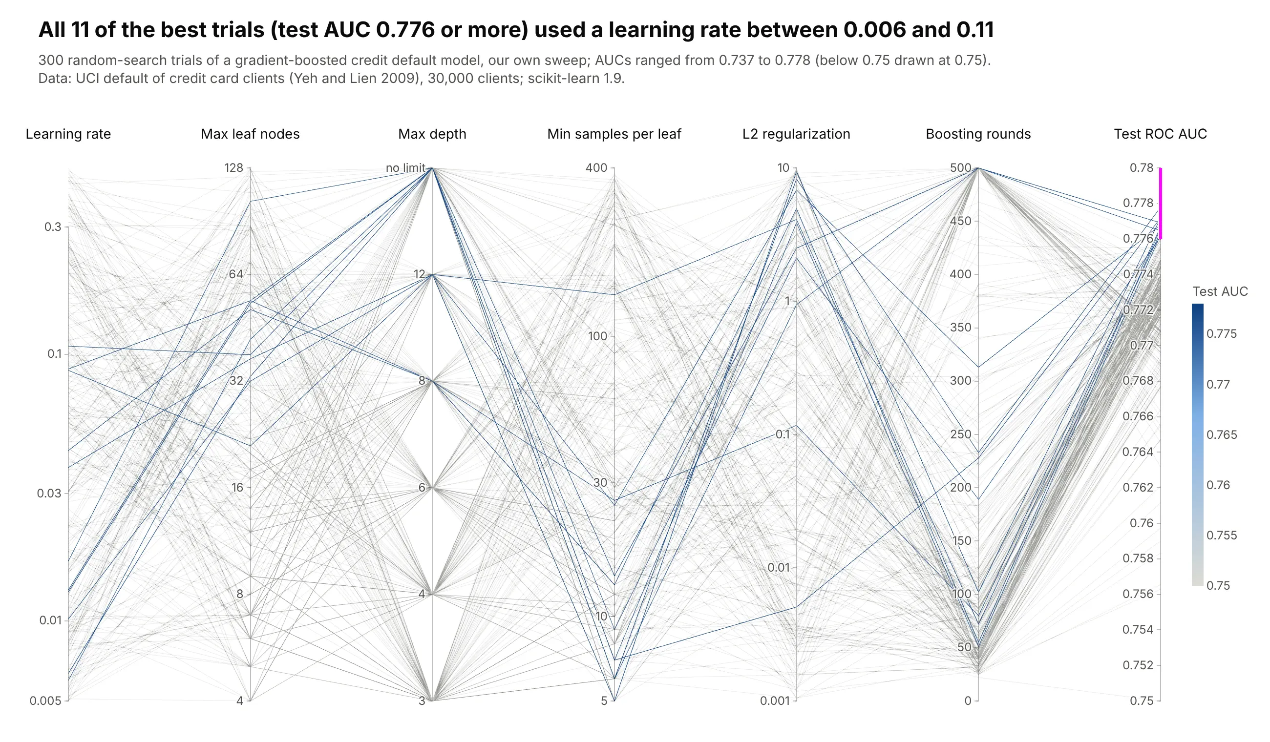
Parallel coordinates of 300 hyperparameter trials across learning rate, max leaf nodes, max depth, min samples per leaf and L2 (log axes), boosting rounds and test AUC, brushed to AUC of 0.776 or more: 11 blue lines

A hyperparameter search. In our 300-trial random search of a gradient-boosted credit default model, the 11 best trials (test AUC 0.776 or more) all used a learning rate between 0.006 and 0.11. Data: our sweep with scikit-learn on UCI's default of credit card clients (Yeh and Lien 2009).

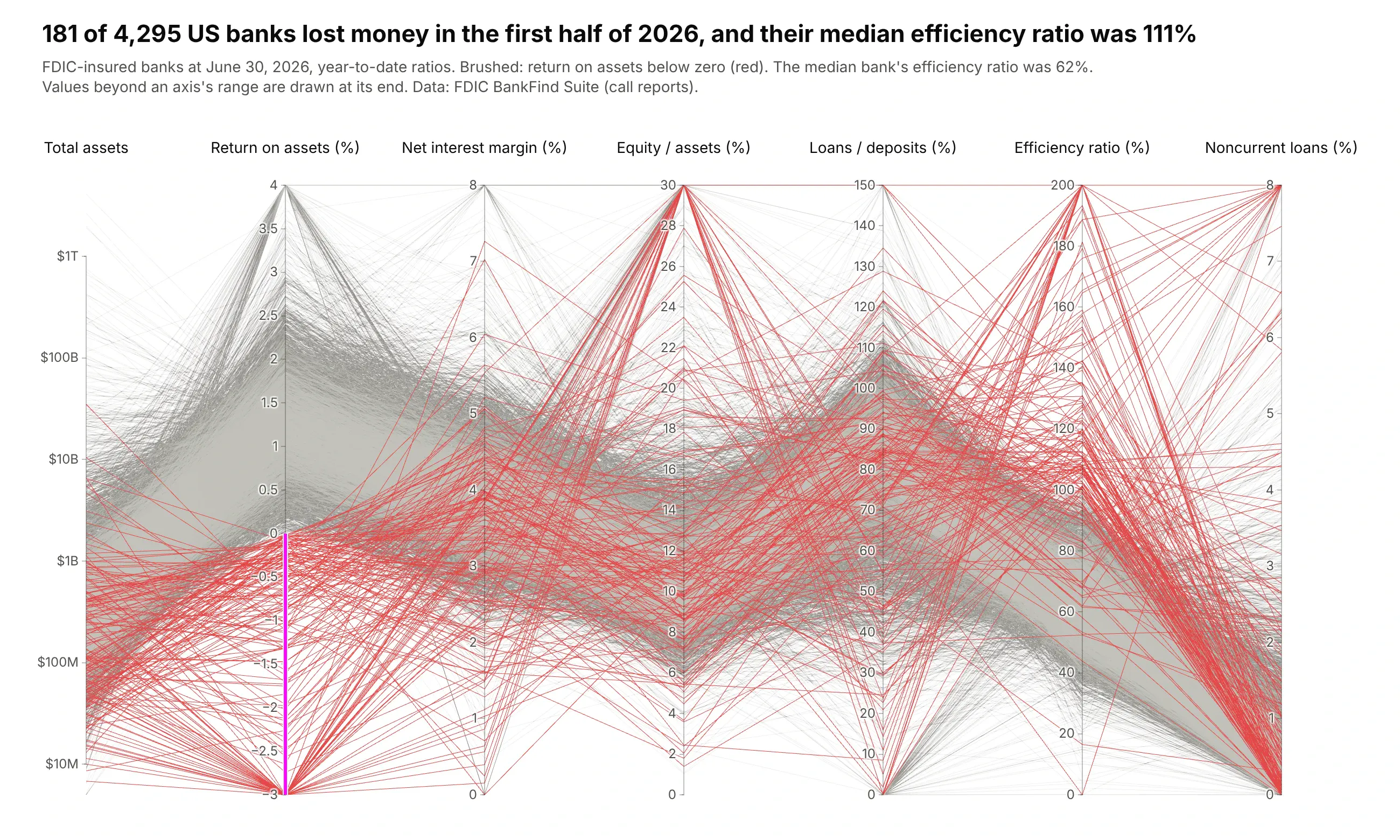
Parallel coordinates of 4,295 US banks across assets, return on assets, margin, capital, loans to deposits, efficiency ratio and noncurrent loans, brushed to negative return on assets: 181 red lines, most with efficiency ratios above 100%

A screen of financial ratios. 181 of 4,295 US banks lost money in the first half of 2026, and their median efficiency ratio was 111% (costs above revenue) against 62% for all banks. Data: FDIC BankFind Suite (call reports), June 30, 2026.

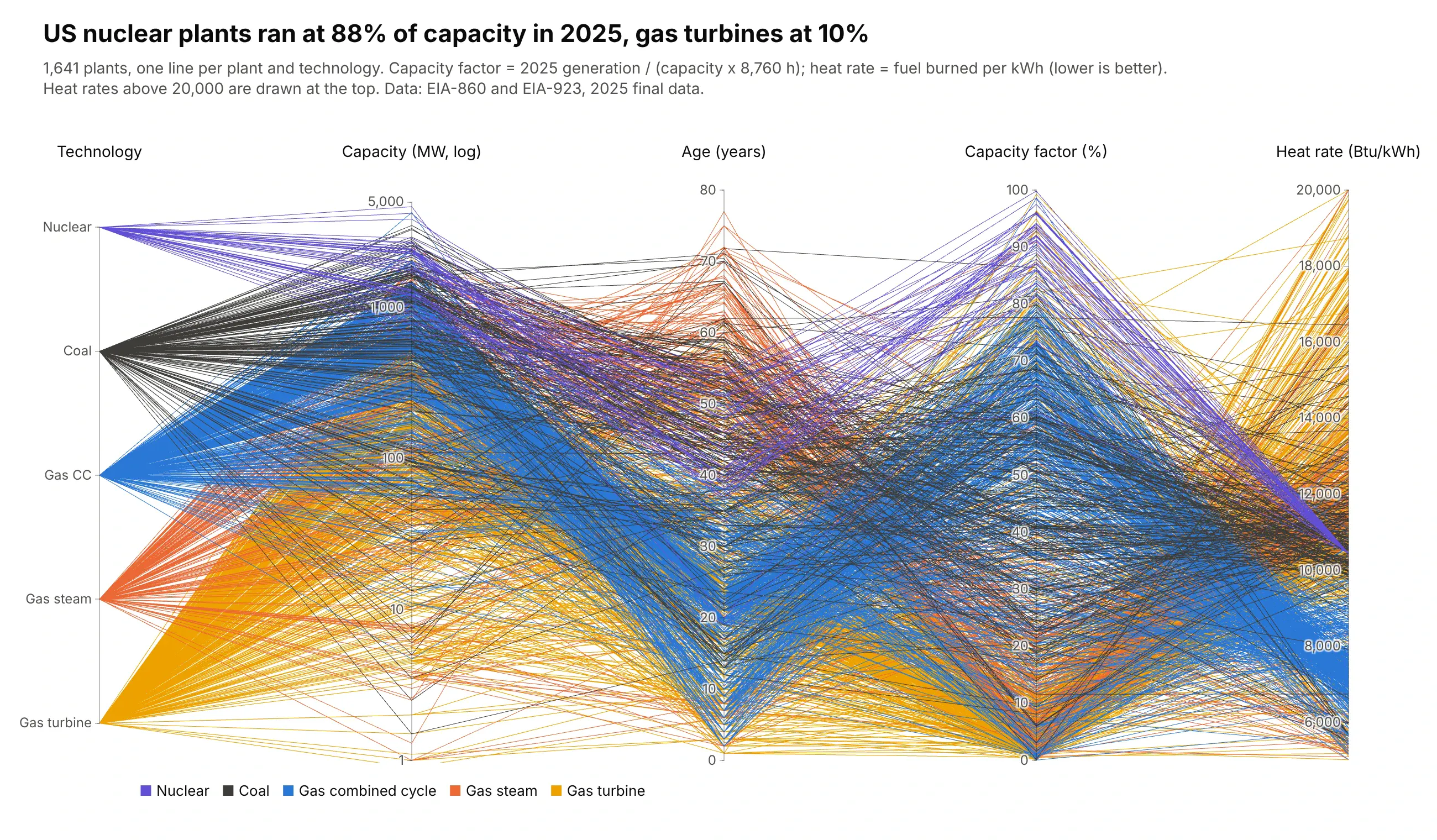
Parallel coordinates of 1,641 US nuclear, coal and gas plants across technology, capacity, age, capacity factor and heat rate. Nuclear plants (purple) run at 80-100% capacity factor; gas turbines (yellow) mostly below 20%

A fleet of assets compared on several measures. In 2025, the 53 US nuclear plants ran at 88% of their capacity and the 679 simple-cycle gas turbine plants at 10%. Data: EIA-860 and EIA-923, 2025 final data.

A short history

Alfred Inselberg made parallel coordinates a tool for multidimensional geometry in "The plane with parallel coordinates" (The Visual Computer, 1985). The paper starts from a duality: the points of a straight line in ordinary x-y coordinates become lines that all pass through one point in parallel coordinates.

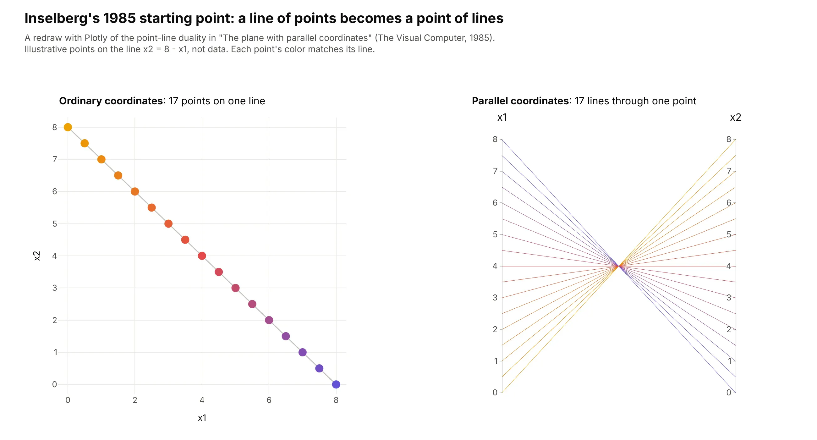
Left, 17 points on the straight line x2 = 8 - x1 in ordinary coordinates, colored from orange to purple. Right, the same 17 points as lines between two parallel axes x1 and x2, all crossing at one point halfway between the axes at the value 4

Edward Wegman brought the method into statistics in "Hyperdimensional data analysis using parallel coordinates" (JASA, 1990), with brushing and the observation that axis order matters. Kosara, Bendix and Hauser adapted it to categorical data as Parallel Sets in 2006, which is what Plotly's go.Parcats draws.

Alternatives to a parallel coordinates plot

Here's the same table of 20 years of risk and return for 49 US industries drawn six ways. Some are better for the question, some worse, some just different:

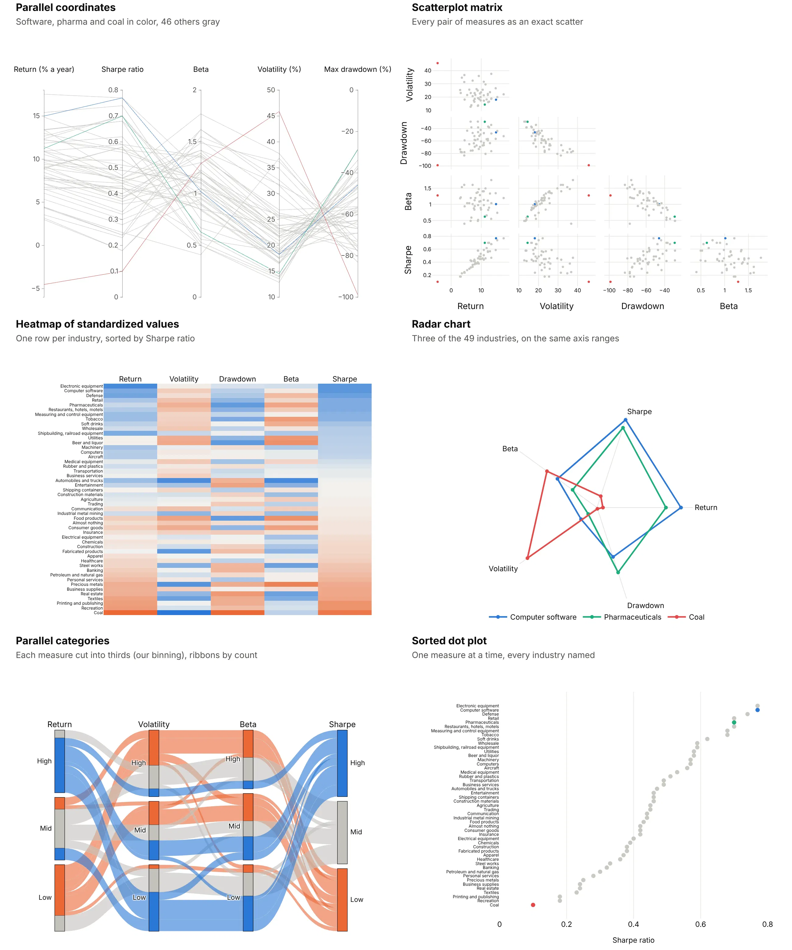
The same 49 US industries drawn six ways: a parallel coordinates plot with software, pharma and coal in color; a scatterplot matrix of the five measures; a heatmap of standardized values sorted by Sharpe ratio; a radar chart of software, pharma and coal; a parallel categories diagram of each measure cut into thirds; and a dot plot of Sharpe ratios with every industry named

Scatterplot matrix (better for exact pairwise relationships). Every pair of measures gets its own scatter, and people read correlation from a scatter more accurately than from lines between parallel axes (Harrison et al., 2014). One industry becomes ten dots, though, so you can't follow it across all five measures. See our scatter plot matrix guide.
Heatmap of standardized values (better when names matter). One row per industry keeps every name readable, but each value becomes a shade, so exact levels are hard to compare. See our heatmap guide.
Radar chart (works too, for a few records). It's parallel coordinates bent into a circle. Three industries are clear, with coal's 46% volatility pulling its shape out to one side, but 49 overlapping shapes would not be. See our radar chart guide.
Parallel categories diagram (different). It's the version for categorical columns, with ribbons sized by counts instead of one line per record. Cutting numbers into bins (here thirds, our binning) throws away detail, so use it when the columns really are categories.
Sorted dot plot (better for one measure). It names every industry and compares one measure precisely, with coal's Sharpe ratio of 0.10 at the bottom and software and electronic equipment tied at 0.77 at the top. It can't show how the five measures relate.

How to make a parallel coordinates plot

With AI

ChatGPT, Claude Code, GitHub Copilot, Cursor and other AI tools are excellent at writing Plotly code. Name Plotly in the prompt, list the axes in the order you want, and say what to brush and what to check:

Make a plotly parallel coordinates plot from screen.csv
(columns: compound_id, mw, logp, hbd, hba, psa, potency_nm).

- Axes in this order: potency (log10, ticks 1-10,000 nM), mw, logp, hbd, hba, psa.
- Fixed ranges; clip outliers to the axis ends and say so in the subtitle.
- constraintrange on mw 0-500 and logp up to 5; no tickvals on brushed axes.
- Selected lines in #6250d6, unselected lines light gray with opacity 0.3.
- Inter font, white background, a title that states how many compounds pass.
- Save it as HTML and as a 2x PNG (draw it in a browser page and screenshot it if kaleido is slow).

With Plotly Studio

Plotly Studio is a desktop app where you point an AI at a dataset and it builds charts and a Dash app around your questions. Ask for a parallel coordinates plot by naming the measures, the order and what to brush:

Show a parallel coordinates plot of every bank in this call report file with total assets (log scale), return on assets, net interest margin, equity to assets, loans to deposits and efficiency ratio. Brush return on assets below zero and gray out the other banks. Add a table below that lists the banks inside the brush.

Make a parallel coordinates plot in Python or JavaScript

This is the code AI tools write under the hood. In Python, px.parallel_coordinates(df, color="petal_length") draws every numeric column in one line, and go.Parcoords gives you fixed ranges, units and a brush:

import plotly.express as px
import plotly.graph_objects as go

df = px.data.iris()
fig = go.Figure(go.Parcoords(
    line=dict(color=df["species_id"], colorscale=[[0, "#2a78d6"], [0.5, "#eb6834"], [1, "#1baf7a"]]),
    dimensions=[
        dict(label="Sepal length (cm)", values=df["sepal_length"], range=[4, 8]),
        dict(label="Sepal width (cm)", values=df["sepal_width"], range=[2, 4.5]),
        dict(label="Petal length (cm)", values=df["petal_length"], range=[1, 7], constraintrange=[4.5, 7]),
        dict(label="Petal width (cm)", values=df["petal_width"], range=[0, 2.5]),
    ],
    unselected=dict(line=dict(color="#c3c2bc", opacity=0.3)),
))
fig.show()

In JavaScript, plotly.js takes one entry per axis, each with its values for every record:

<div id="chart"></div>
<script src="https://cdn.plot.ly/plotly-4.1.1.min.js"></script>
<script>
  Plotly.newPlot("chart", [{
    type: "parcoords",
    line: {color: [0.77, 0.70, 0.58, 0.32, 0.10], colorscale: [[0, "#c3c2bc"], [1, "#2a78d6"]]},
    dimensions: [
      {label: "Return (% a year)", values: [14.99, 11.23, 9.00, 6.54, -4.53], range: [-6, 18]},
      {label: "Volatility (%)", values: [18.24, 14.54, 13.93, 23.30, 45.87], range: [10, 50]},
      {label: "Max drawdown (%)", values: [-45.92, -28.88, -37.91, -75.23, -98.68], range: [-100, 0]},
      {label: "Sharpe ratio", values: [0.77, 0.70, 0.58, 0.32, 0.10], range: [0, 0.8], constraintrange: [0.5, 0.8]}
    ]
  }]);
</script>

The five lines are software, pharmaceuticals, utilities, banking and coal from the alternatives figure above.

Share it

Every Plotly chart has a Share chart button (the cloud icon in its toolbar) that uploads it to Plotly Cloud and gives you a link. Only you can see it until you change its visibility.

For a live app, put the chart in a Dash app and publish it with the Plotly Cloud CLI. In Dash, the graph's restyleData reports every brush change, so a callback can filter a table to the selected rows. Coding agents can run these commands for you:

pip install "dash[cloud]"
plotly user login
plotly app publish

If your data has to stay in your own cloud or data center, publish to Dash Enterprise instead.

Dos and don'ts

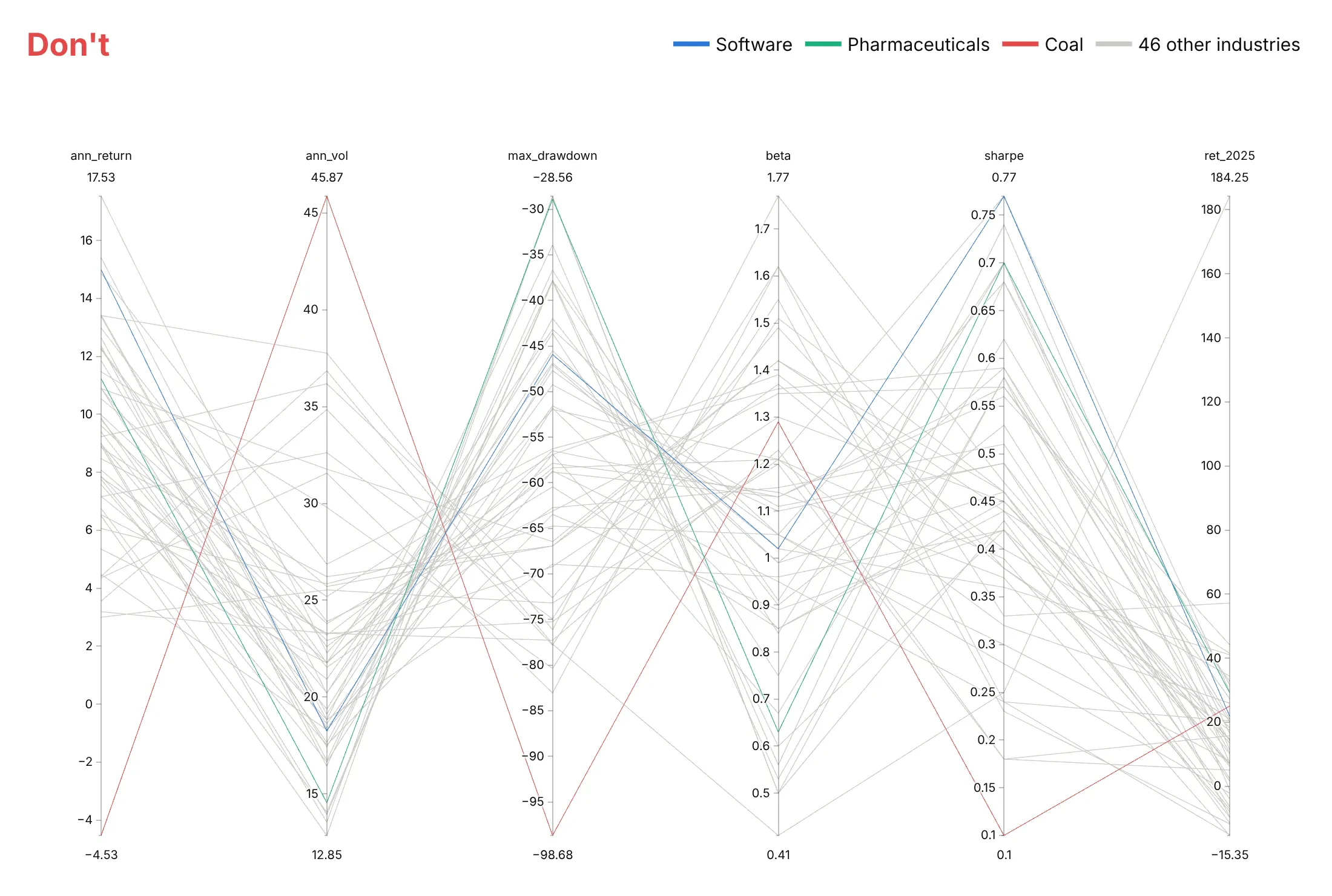
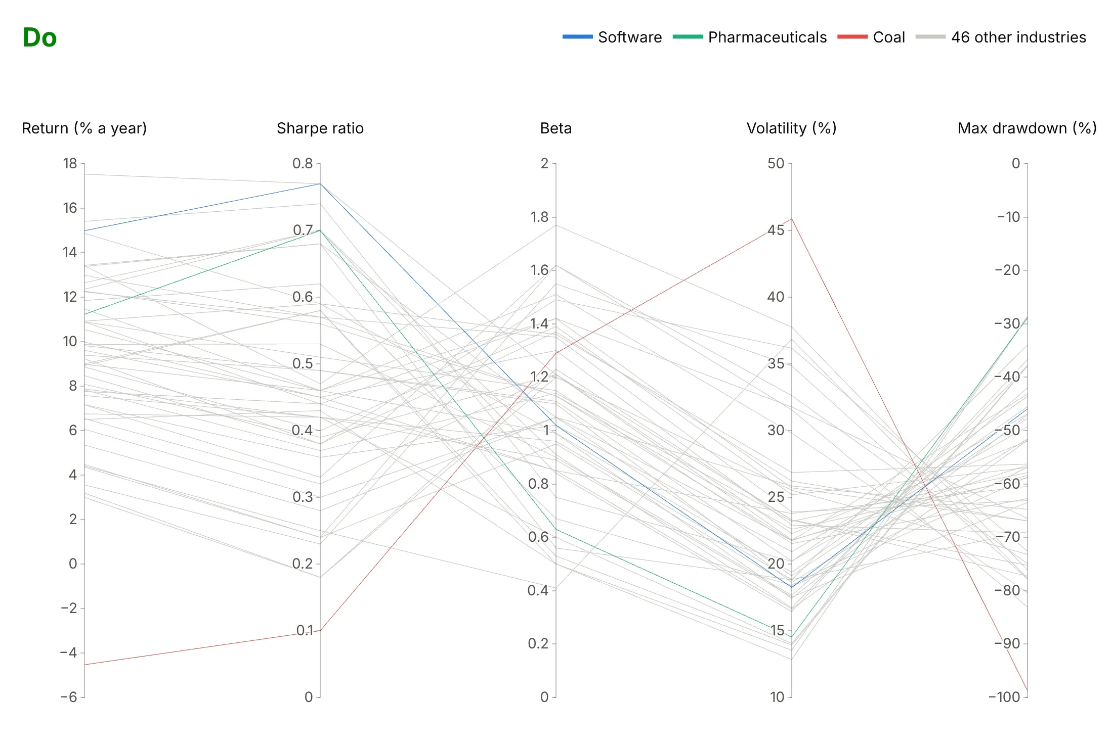
Plotly's defaults are made for exploring a file. For a published chart, most of the work is choosing the axes, their order and their ranges. Here are the same 49 industries both ways, with the same colors in both.

Don't keep every column in file order with raw column names and autoranged axes. Each axis then stretches to its own minimum and maximum, so the drawdown axis runs from -28.56 to -98.68 instead of from 0, the min and max labels crowd the axis titles, and a column that doesn't answer the question (the 2025 return, stretched to 184 by precious metals) takes a sixth of the width:

A parallel coordinates plot of 49 US industries with software in blue, pharmaceuticals in green, coal in red and the rest gray, but with raw column names such as ann_return and max_drawdown, small fonts, min and max labels such as -98.68 above and below every axis, autoranged axes, and a last ret_2025 axis stretched to 184

Do put units in the labels, fix the ranges, put return next to Sharpe ratio, drop the column that doesn't answer the question, and use fonts that can be read on a phone:

The same 49 industries and the same colors designed on purpose: axes labeled Return (% a year), Sharpe ratio, Beta, Volatility (%) and Max drawdown (%) with fixed ranges such as -100 to 0 for drawdown, larger fonts and no min and max labels

Use color for one thing

Parallel coordinates lines can't carry labels, so color is how readers follow a line across the chart. Here are four options on the same data.

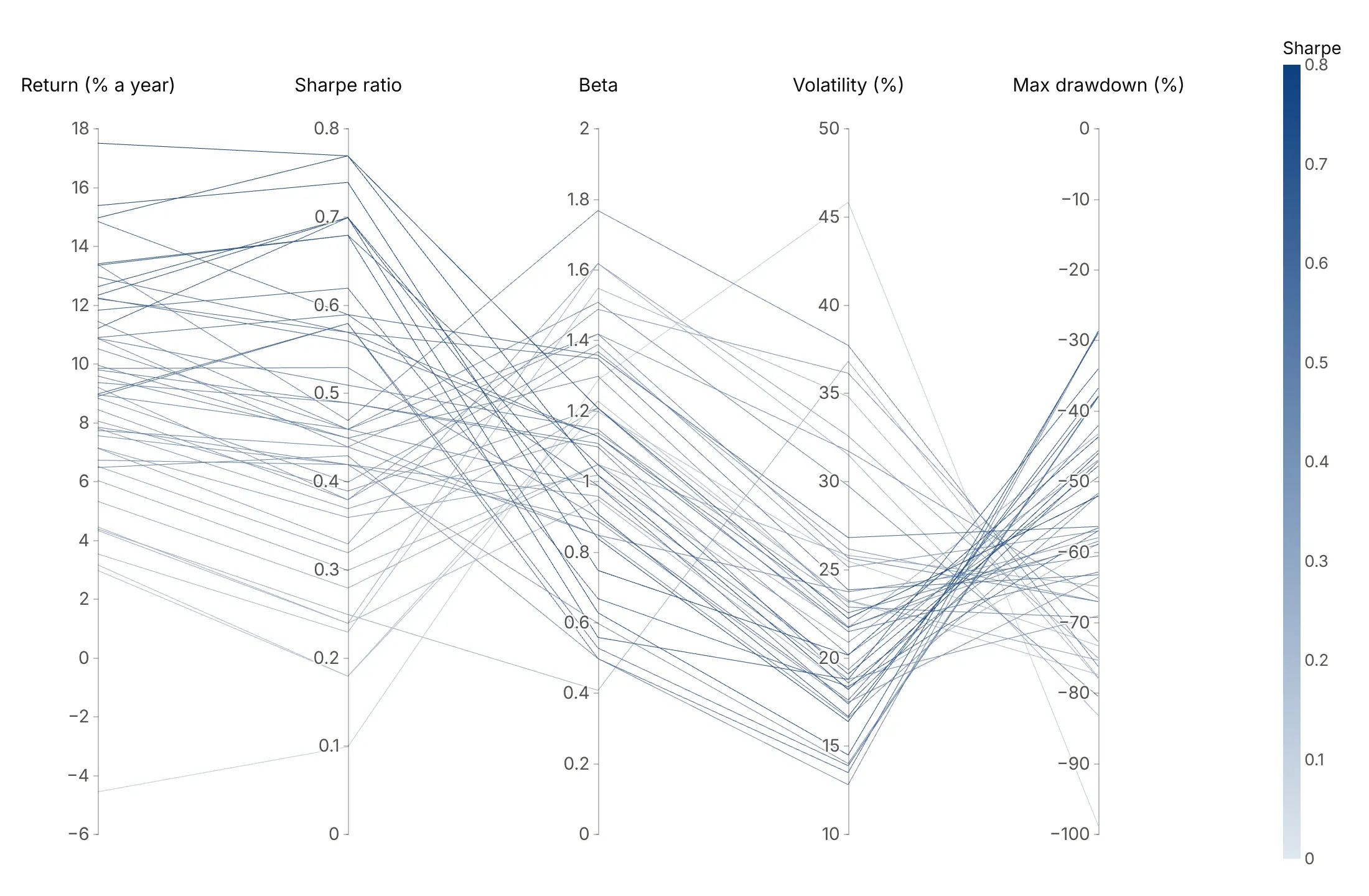
A measure. Light to dark blue by Sharpe ratio shows how the best risk-adjusted industries sit on every other axis.

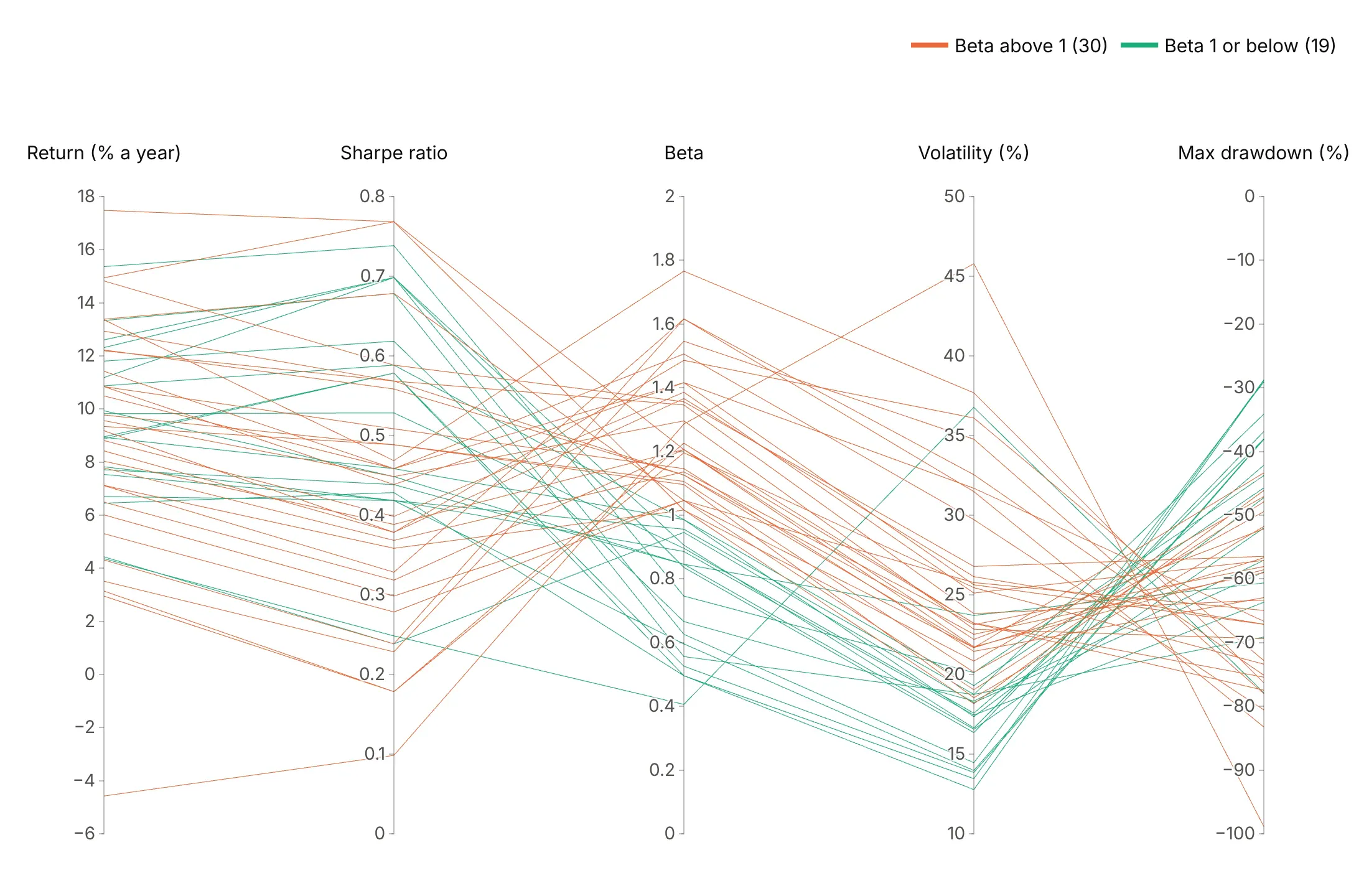
The 49 industries colored from light to dark blue by Sharpe ratio, with a colorbar from 0 to 0.8

A group. Two colors split the 30 industries with a beta above 1 from the 19 at or below it.

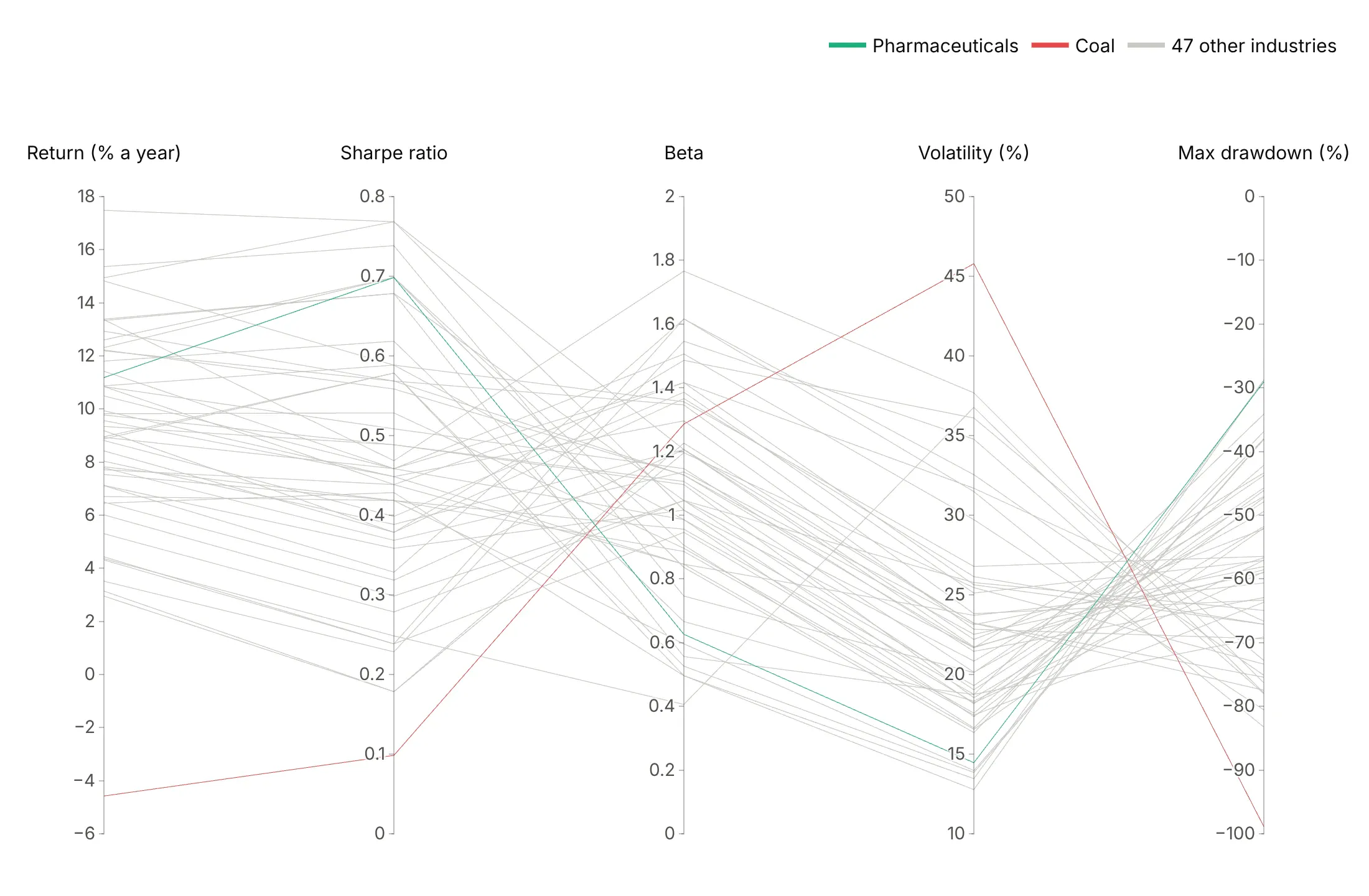
The 49 industries with 30 orange lines for a beta above 1 and 19 green lines for a beta of 1 or below

A highlight. Coal and pharmaceuticals in color and the other 47 in gray tell one story, a 99% drawdown against a 29% one.

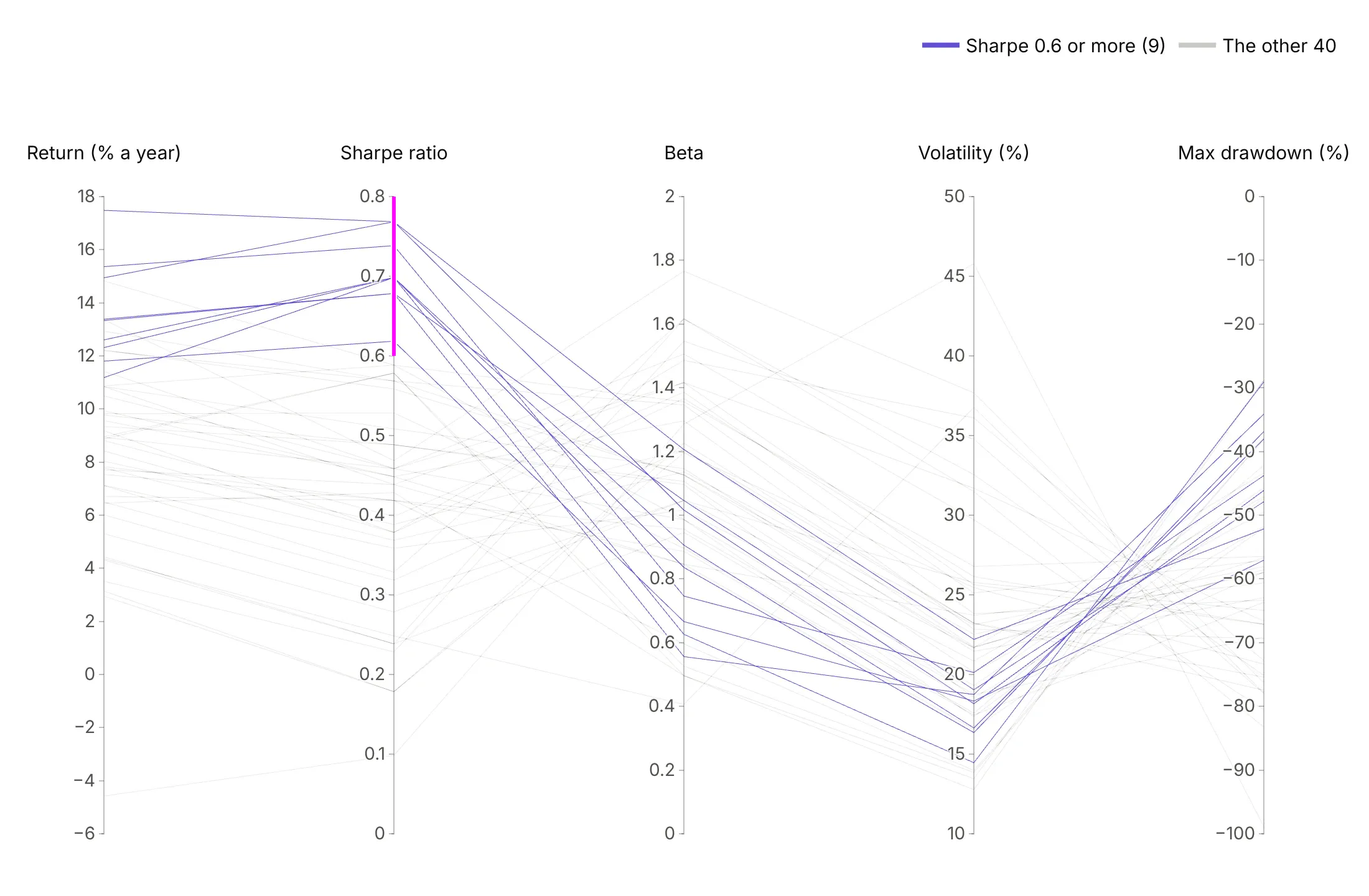
The 49 industries in light gray with coal in red and pharmaceuticals in green

A brush. A brush on the Sharpe axis keeps the 9 industries at 0.6 or more in purple, and in the interactive chart readers can move it.

The 49 industries with a brush on Sharpe ratio from 0.6 to 0.8: 9 purple lines and 40 light gray lines

Checklist

Write a title that states the takeaway, usually the result of a brush.
Order axes on purpose: the filter axis first or last, and pairs you want compared next to each other.
Fix the ranges with range, and use one range for axes in the same units.
Flip axes where lower is better (range=[high, low]) so better is up everywhere.
Show the brushed state in static images with constraintrange, and gray the rest with unselected.line.
Put units in the axis labels and hide the min and max labels when the ticks show the range.

Don't

Keep the default column order, which is the order of your file, not of your question.
Let one outlier set an axis. Clip to a fixed range and say so in the subtitle.
Use a rainbow for groups or for a measure.
Rely on hover, because parcoords has no per-line hover. Name the records that matter in the text.
Use parcoords for categories, because integer-coded categories pile onto a few ticks. Use go.Parcats.

Options to customize

These are the go.Parcoords (and px.parallel_coordinates) and go.Parcats options that matter most. The full references are the parallel coordinates and parallel categories docs.

dimensions (px: a list of columns): the axes and their order, the main design decision.
dimensions[].label, .values: the axis title and data. Put units in the label.
dimensions[].range: a fixed axis range; [high, low] flips the axis so better is up.
dimensions[].constraintrange: a brush, or a list of ranges, for static brushed images and initial filters.
dimensions[].multiselect: allows several brushes on one axis, for OR filters.
dimensions[].tickvals, .ticktext: custom ticks for log10 axes and categories. Keep them off brushed axes.
dimensions[].tickformat: a d3 number format such as $, or .0%.
dimensions[].visible: hides an axis but keeps its brush, to filter on a column you don't show.
line.color, colorscale, cmin, cmax: line color from a number, for a measure, a group (stepped scale) or a highlight.
line.showscale, colorbar: the color legend, when color is a continuous measure.
unselected.line.color, .opacity: the style of lines outside a brush, usually faint gray.
labelangle, labelside: the axis title angle and position, for long labels.
labelfont, tickfont, rangefont: fonts; rangefont styles the min and max labels.
domain: where the plot sits in the figure, to leave room for titles and notes.
Parcats dimensions[].categoryorder, categoryarray: the category order on an axis, for ordinal categories such as age bands.
Parcats counts: the ribbon size per row, for pre-aggregated data.
Parcats line.color, line.shape: ribbon color, and hspline for curved ribbons.
Parcats arrangement, sortpaths, bundlecolors: drag behavior, ribbon order and color bundling, for fewer crossings.

More parallel coordinates examples

Ten more parallel coordinates plots and parallel categories diagrams built from real public data, each with its source, the technique that makes it work and a prompt to rebuild it.

1. Which generators are scheduled to retire

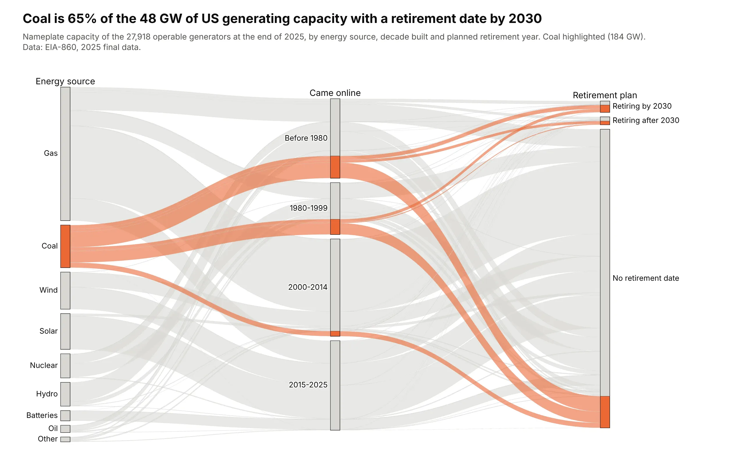
Parallel categories diagram of 1,377 GW of US generating capacity by energy source, decade built and retirement plan, with coal ribbons in orange: most coal came online before 2000 and most of it has no retirement date

Of the 48 GW of US capacity with a retirement date by 2030, 31 GW (65%) is coal. Most coal still has no retirement date: 137 of its 184 GW. Data: EIA-860, 2025 final data.

Tip: go.Parcats with counts= sizes ribbons by gigawatts instead of generator counts, and a two-color colorscale highlights one source.

Get the data from EIA-860 2025 (eia.gov), sheet "Operable" of the generator file, and shape it
into a table (columns: source, era [before 1980, 1980-1999, 2000-2014, 2015-2025],
retirement [by 2030, after 2030, no date], capacity_mw).

Build a plotly go.Parcats with counts=capacity in GW and categoryorder="array" on every axis.
- Coal ribbons orange, everything else light gray; hspline ribbons.
- Title with coal's share of capacity retiring by 2030.

2. Rich countries with clean electricity

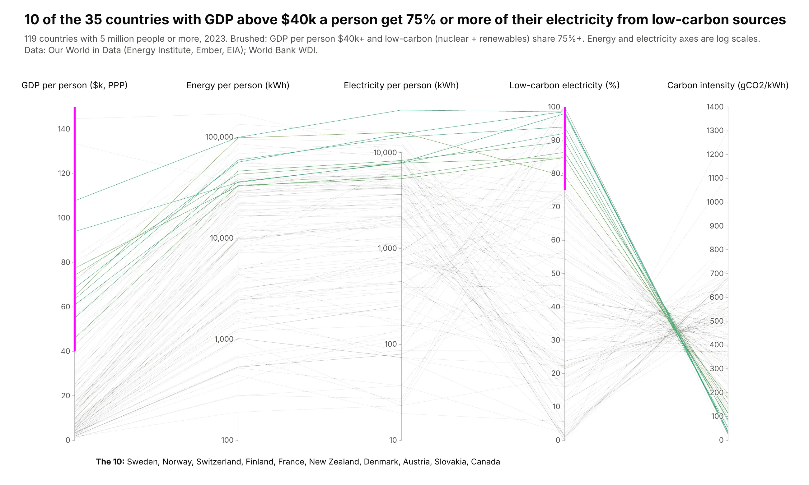
Parallel coordinates of 119 countries with GDP per person, energy and electricity per person on log scales, low-carbon share and carbon intensity, brushed to GDP above $40,000 and low-carbon share above 75%: 10 green lines remain

Of 35 countries with GDP above $40,000 a person, 10 get 75% or more of their electricity from nuclear and renewables, from Norway and Sweden to France and Slovakia. Their lines all end below 200 gCO2/kWh. Data: Our World in Data (Energy Institute, Ember, EIA) and World Bank, 2023.

Tip: two constraintrange brushes make an AND filter, and the brushed GDP axis stays linear because a brush on an axis with tickvals snaps to the ticks.

Get the data from Our World in Data's energy dataset (github.com/owid/energy-data) and World Bank
GDP per person, PPP (NY.GDP.PCAP.PP.CD), 2023, and shape it into a table (columns: country,
gdp_pc_ppp, energy_pc_kwh, elec_pc_kwh, low_carbon_share, carbon_intensity), countries with 5M+ people.

Build a plotly go.Parcoords with GDP ($k, linear), energy and electricity per person (log10 with
tickvals), low-carbon share and carbon intensity.
- constraintrange on GDP >= 40 and low-carbon share >= 75; unselected lines light gray.
- List the matching countries under the chart; title with the count.

3. Every Treasury yield curve since 1982

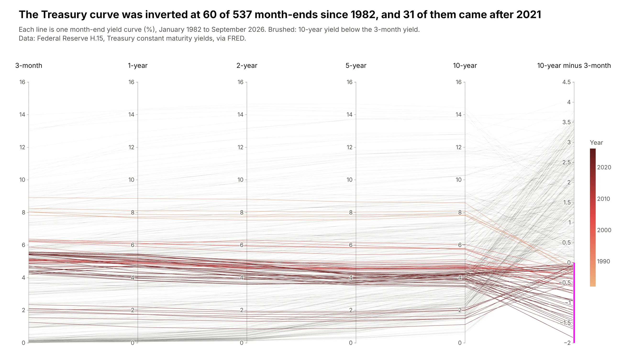
Parallel coordinates of 537 month-end Treasury yield curves from 3-month to 10-year plus the 10-year minus 3-month spread, brushed to inverted curves: 60 colored lines, the darkest from 2022-2024

With maturities as axes, each line is a yield curve. Brushing the spread below zero leaves 60 inverted month-ends since 1982, and 31 of them came after 2021. Data: Federal Reserve H.15 via FRED.

Tip: the five yield axes share one 0-16% range, so the slope of a line between axes is the real slope of the curve.

Get the data from FRED (Federal Reserve H.15): DGS3MO, DGS1, DGS2, DGS5, DGS10, month-end
values from 1982, and shape it into a table (columns: date, year, y3m, y1, y2, y5, y10,
spread_10y_3m).

Build a plotly go.Parcoords: five yield axes with the same 0-16 range, then the spread.
- Color by year (light orange to dark red) with a colorbar.
- constraintrange on the spread below 0; faint gray unselected lines. Title with the count.

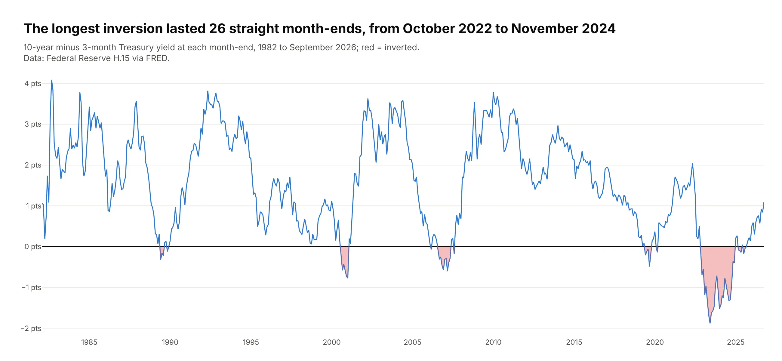
Another way to see it: a line chart of the spread over time shows when the inversions happened, including the longest, 26 straight month-ends from October 2022 to November 2024.

Line chart of the 10-year minus 3-month Treasury spread at each month-end from 1982 to 2026, with inversions shaded red; the longest ran from October 2022 to November 2024

4. NHANES adults with diabetes-range HbA1c

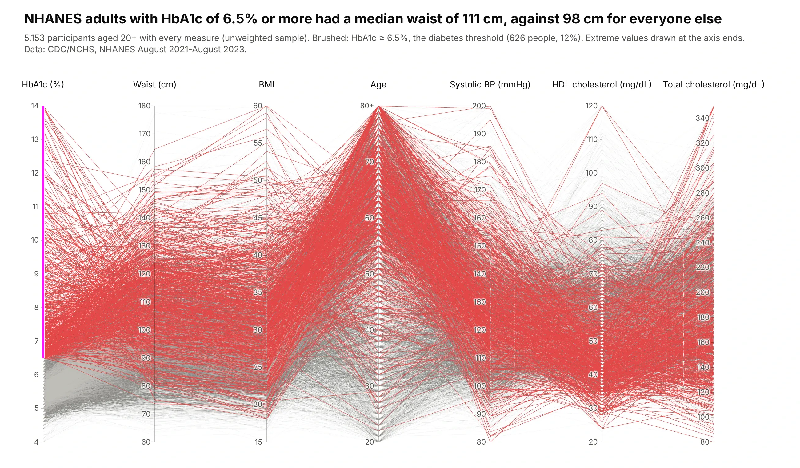
Parallel coordinates of 5,153 NHANES adults across HbA1c, waist, BMI, age, blood pressure, HDL and total cholesterol, brushed to HbA1c of 6.5% or more: 626 red lines, higher on waist and BMI

Brushing HbA1c at 6.5% and above leaves 626 of 5,153 adults (12%). Their median waist is 111 cm against 98 cm for everyone else, and their lines sit high on BMI and low on HDL. Data: CDC/NCHS, NHANES August 2021-August 2023, unweighted.

Tip: the brushed axis goes first and the axes most related to it (waist, BMI) next to it, so the eye reads the filter and then its effect.

Get the data from NHANES August 2021-August 2023 (wwwn.cdc.gov/nchs/nhanes): DEMO_L, BMX_L,
BPXO_L, TCHOL_L, HDL_L, GHB_L, and shape it into a table (columns: age, bmi, waist_cm, sys,
hdl, total_chol, hba1c), adults 20+.

Build a plotly go.Parcoords with HbA1c first, then waist, BMI, age, systolic BP, HDL, total
cholesterol. constraintrange HbA1c >= 6.5; red selected lines, unselected opacity 0.12.
Say "unweighted sample" in the subtitle.

5. From BMI to HbA1c, as categories

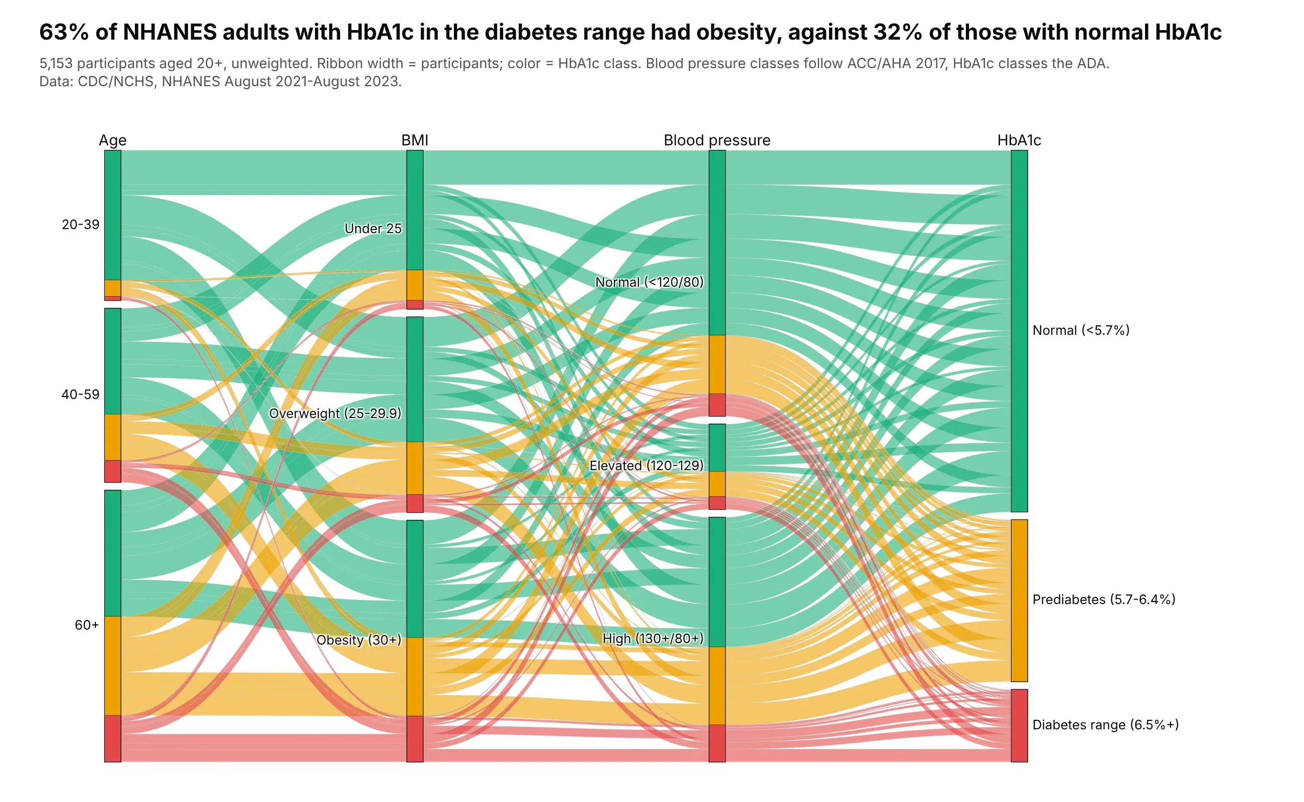
Parallel categories diagram of 5,153 NHANES adults by age group, BMI class, blood pressure class and HbA1c class, ribbons colored by HbA1c class from green to red

As categories, the same NHANES adults show that 63% of those with diabetes-range HbA1c had obesity, against 32% of those with normal HbA1c. Data: CDC/NCHS, NHANES August 2021-August 2023, unweighted.

Tip: ribbons are colored by the last axis, so each outcome can be traced back to the left.

Get the data from NHANES August 2021-August 2023 (as in the previous example) and shape it into
a table of counts (columns: age_group, bmi_class, bp_class [ACC/AHA 2017], hba1c_class [ADA],
participants).

Build a plotly go.Parcats with counts=participants, categories in clinical order, ribbons
colored by HbA1c class (green, amber, red). Title with the obesity share by HbA1c class.

6. Who posts clinical trial results

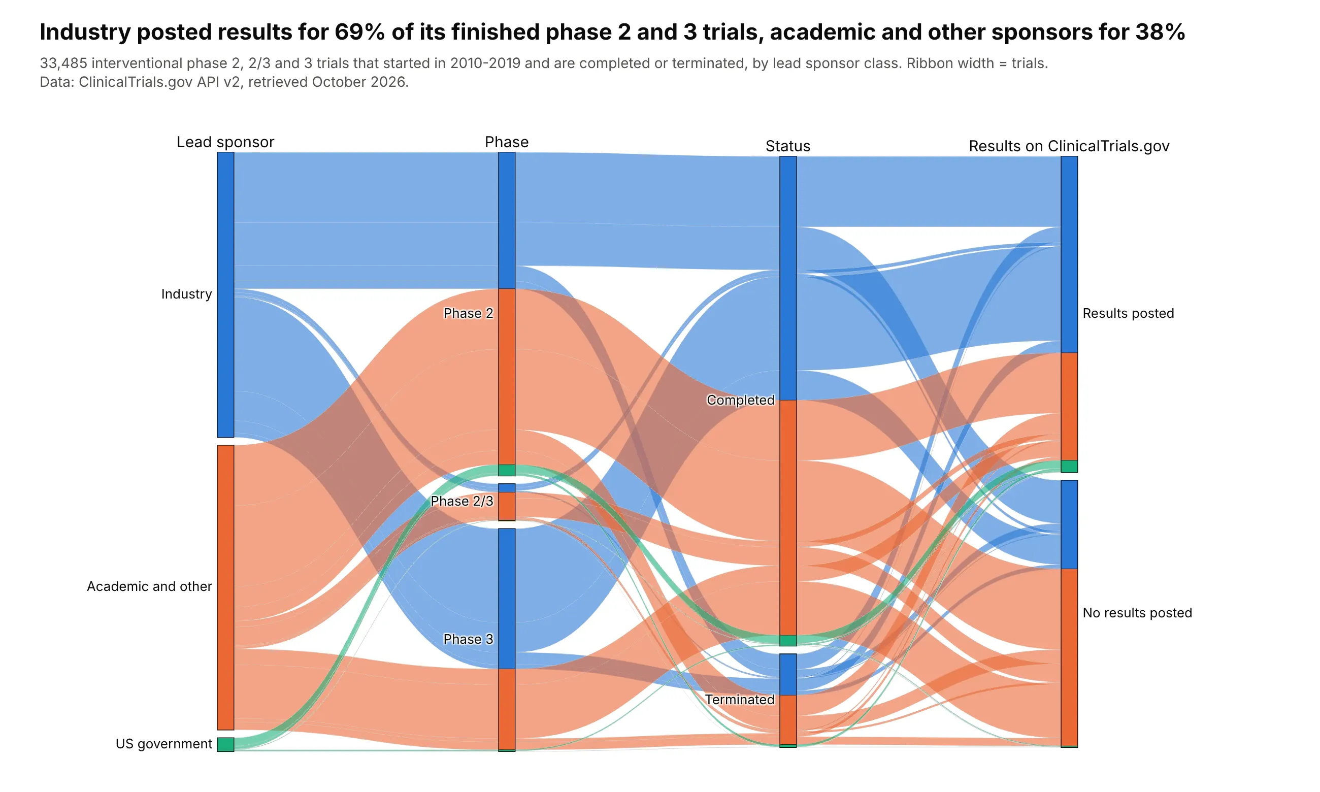
Parallel categories diagram of 33,485 finished phase 2 and 3 trials by lead sponsor, phase, status and whether results are on ClinicalTrials.gov; industry ribbons (blue) mostly end in results posted, academic ribbons (orange) mostly in no results

Of 33,485 phase 2 and 3 trials that started in 2010-2019 and have ended, industry posted results on ClinicalTrials.gov for 69% and academic and other sponsors for 38%. Data: ClinicalTrials.gov API v2.

Tip: color follows the first axis, so each sponsor class can be traced to the outcome on the right.

Get the data from the ClinicalTrials.gov API v2 (clinicaltrials.gov/api/v2/studies): interventional
phase 2 and 3 trials that started 2010-2019, completed or terminated, and shape it into a table of
counts (columns: sponsor [Industry, Academic and other, US government], phase, status,
results [posted or not], trials).

Build a plotly go.Parcats with counts=trials, colored by sponsor, sortpaths="forward".
Title with the results-posted rate for industry and academic sponsors.

7. Six LLM benchmarks for 4,565 open models

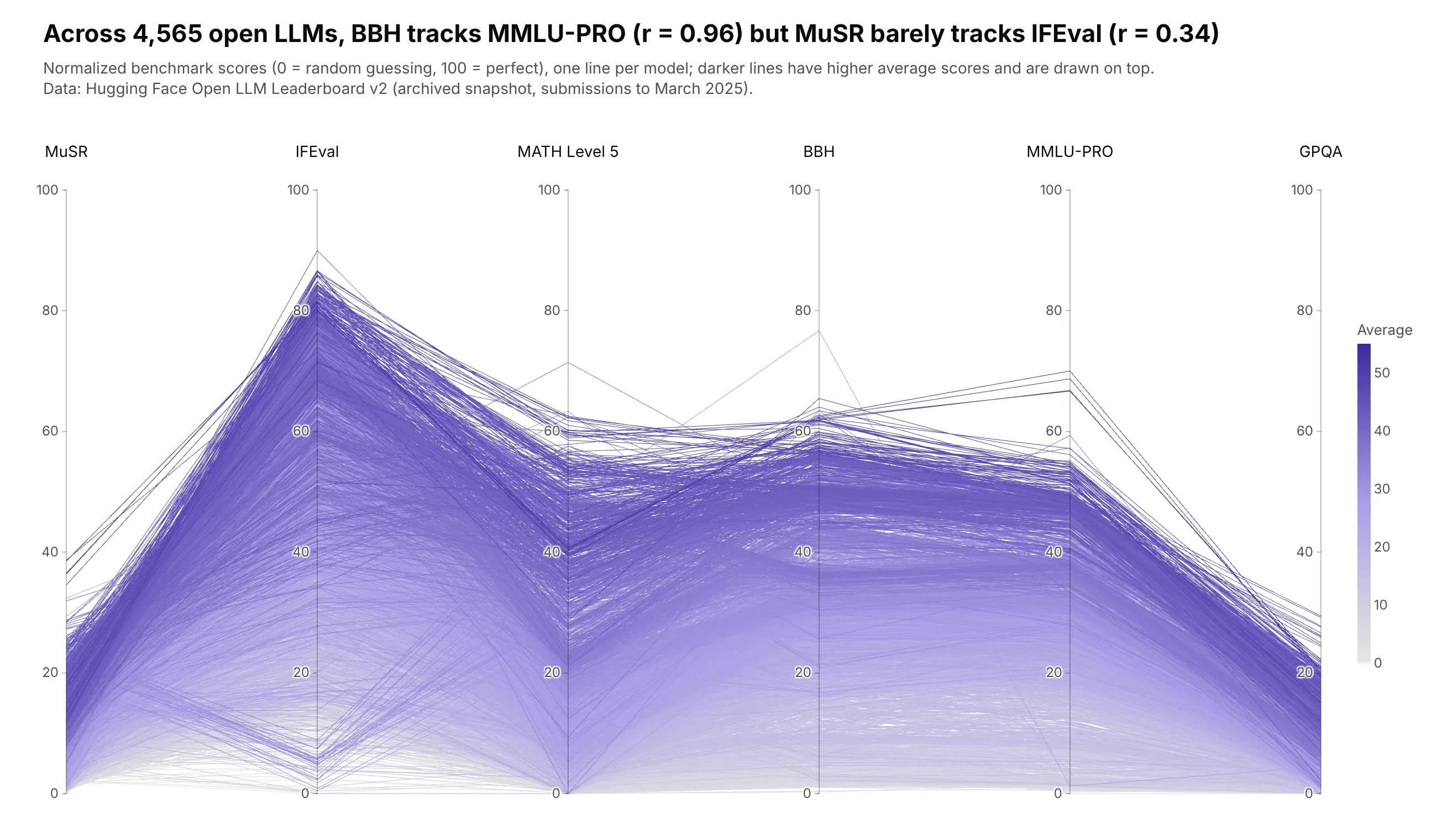
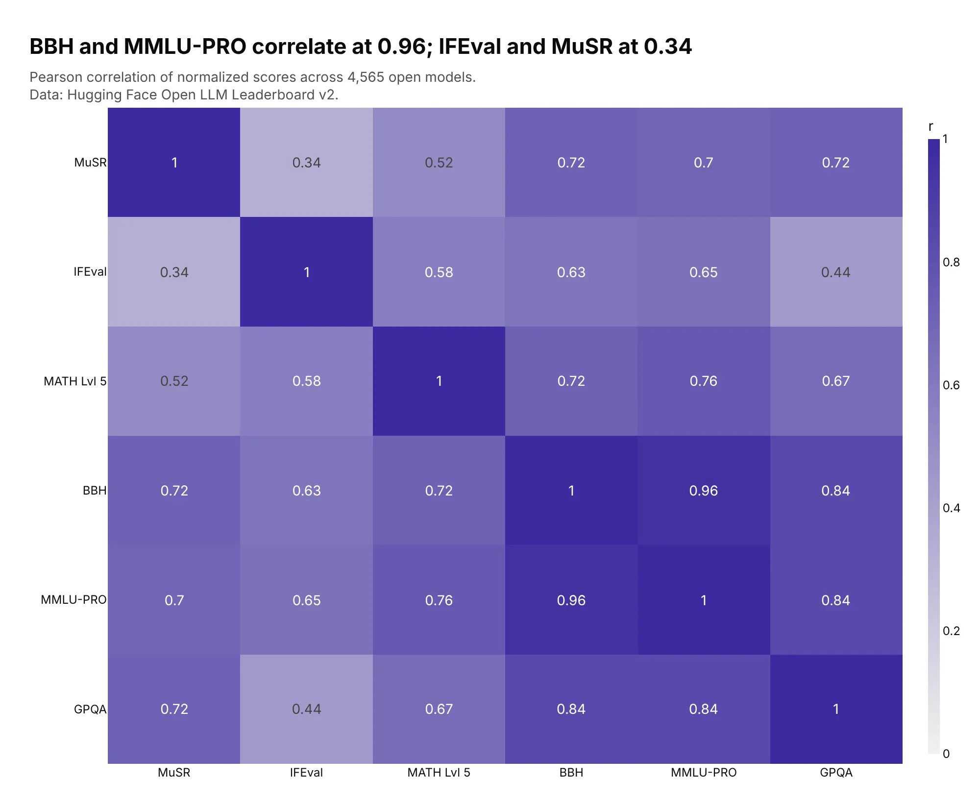
Parallel coordinates of 4,565 open LLMs across MuSR, IFEval, MATH, BBH, MMLU-PRO and GPQA, colored by average score; lines run nearly parallel between BBH and MMLU-PRO and cross heavily between MuSR and IFEval

Axis order decides what you see. BBH and MMLU-PRO scores move together across 4,565 open models (r = 0.96), so lines between them run parallel, while MuSR and IFEval barely relate (r = 0.34), so lines between them cross. Data: Hugging Face Open LLM Leaderboard v2 (archived).

Tip: a sequential colorscale on the average puts the best models on top, because parcoords draws higher color values last.

Get the data from the Hugging Face Open LLM Leaderboard v2 contents dataset (huggingface.co,
open-llm-leaderboard/contents) and shape it into a table (columns: model, musr, ifeval, math,
bbh, mmlu_pro, gpqa, average).

Build a plotly go.Parcoords with all six score axes on 0-100, ordered so BBH and MMLU-PRO are
neighbors and MuSR and IFEval are neighbors. Color by average. Title with both correlations.

Another way to see it: a correlation heatmap gives every pair's r exactly, but not the spread of individual models.

Heatmap of correlations between six LLM benchmarks: BBH and MMLU-PRO 0.96, IFEval and MuSR 0.34

8. Fast 300-pound players at the NFL Combine

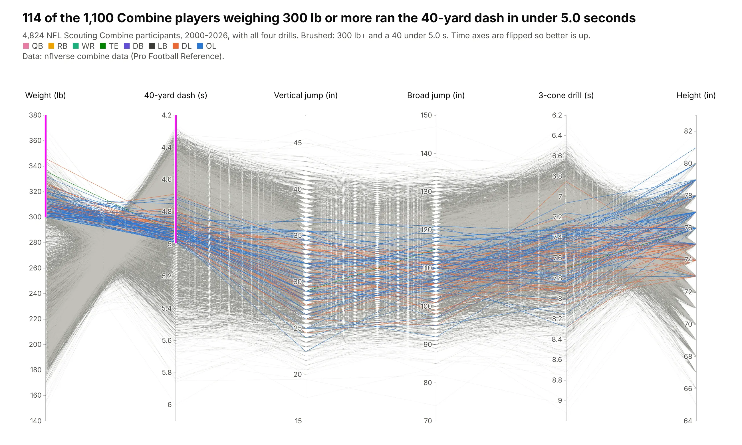
Parallel coordinates of 4,824 NFL Combine players across weight, 40-yard dash, vertical, broad jump, 3-cone and height, brushed to 300 lb or more and a 40 under 5.0 s: 114 lines, mostly offensive and defensive linemen

Of 1,100 Combine players weighing 300 lb or more since 2000, 114 ran the 40-yard dash in under 5.0 seconds, almost all of them linemen. The fastest was Tank Johnson in 2004, 304 lb in 4.69 s. Data: nflverse combine data (Pro Football Reference).

Tip: time axes are flipped with range=[high, low] so better is up on every axis.

Get the data from nflverse's combine.csv (github.com/nflverse/nflverse-data, release "combine")
and shape it into a table (columns: player_name, season, group, weight_lb, forty, vertical,
broad_jump, cone, height_in).

Build a plotly go.Parcoords with the 40 and 3-cone axes reversed; constraintrange weight >= 300
and forty < 5.0; color by position group.

9. Earth-sized, temperate exoplanets

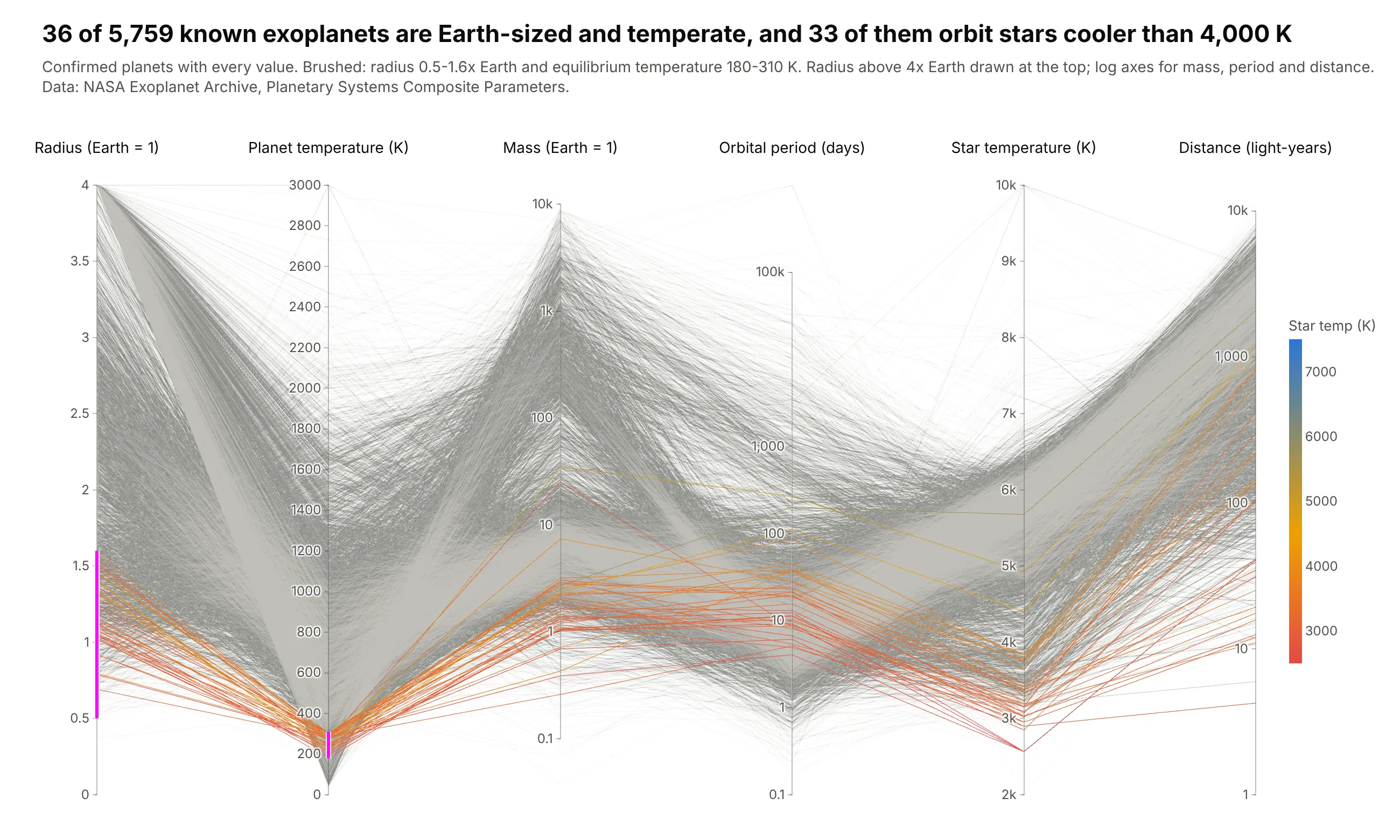
Parallel coordinates of 5,759 exoplanets across radius, temperature, mass, period, star temperature and distance, brushed to 0.5-1.6 Earth radii and 180-310 K: 36 lines, mostly red for cool stars

Of 5,759 confirmed exoplanets with full data, 36 are Earth-sized and temperate, and 33 of those orbit stars cooler than 4,000 K, with a median orbit of 17 days. Data: NASA Exoplanet Archive.

Tip: the brushed radius axis is linear and clipped at 4 Earth radii, while the unbrushed mass, period and distance axes are log10 with tickvals.

Get the data from the NASA Exoplanet Archive (exoplanetarchive.ipac.caltech.edu), table pscomppars,
and shape it into a table (columns: pl_name, pl_rade, pl_eqt, pl_bmasse, pl_orbper, st_teff, sy_dist).

Build a plotly go.Parcoords: radius (linear, clipped at 4), equilibrium temperature, mass,
period and distance (log10 with tickvals), star temperature. constraintrange radius 0.5-1.6
and temperature 180-310; color by star temperature.

10. Fuel cost for every 2026 vehicle

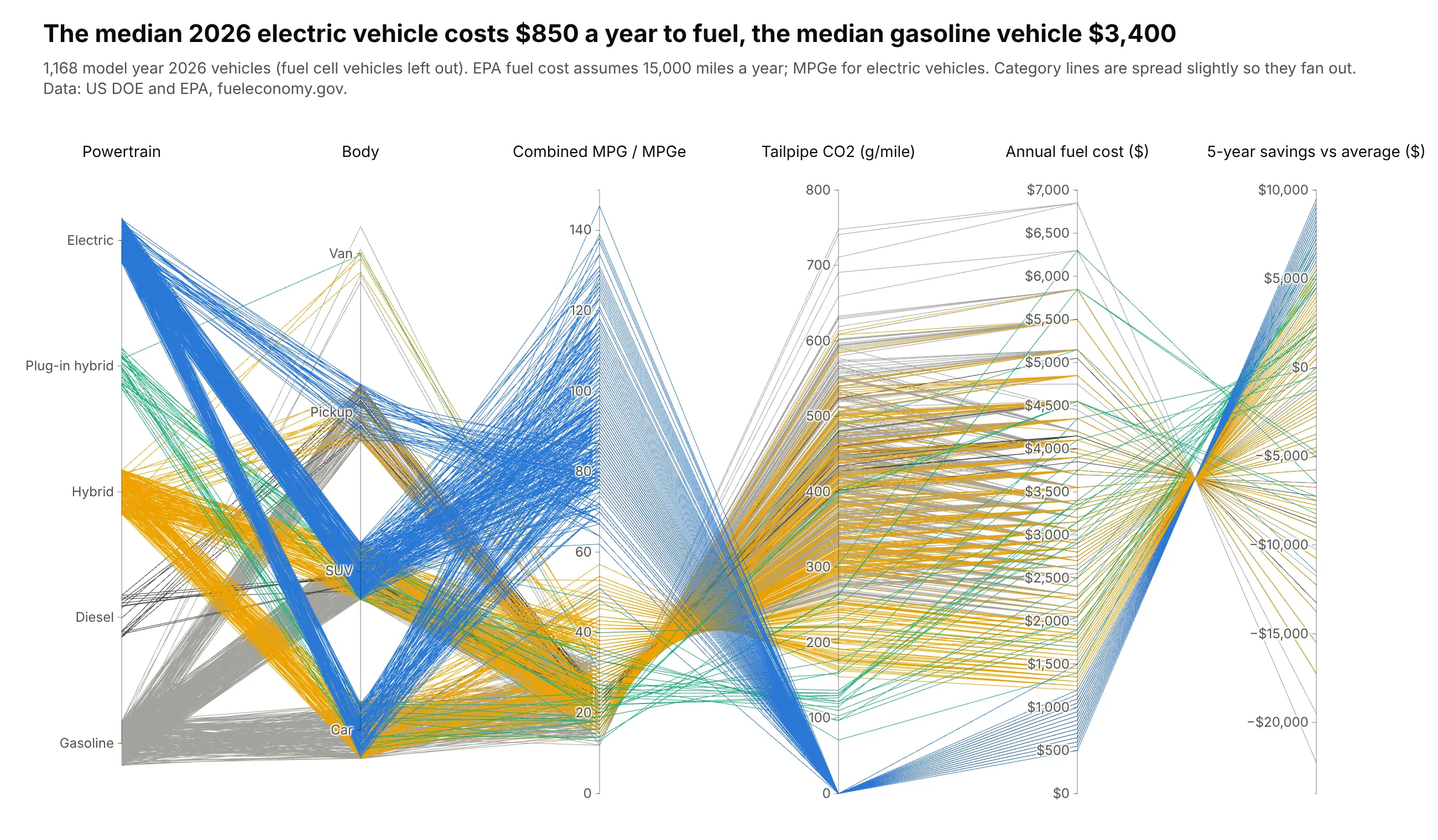
Parallel coordinates of 1,168 model year 2026 vehicles across powertrain, body, MPG or MPGe, CO2, annual fuel cost and five-year savings; electric vehicles (blue) run from zero CO2 to the lowest fuel costs

The median 2026 electric vehicle costs $850 a year to fuel and the median gasoline vehicle $3,400. Because EPA's five-year savings is computed from the fuel cost, every line crosses at one point between those two axes, the same duality Inselberg described in 1985. Data: US DOE and EPA, fueleconomy.gov.

Tip: categorical axes with a little jitter fan lines out instead of meeting at a single point.

Get the data from fueleconomy.gov vehicles.csv (fueleconomy.gov/feg/epadata), model year 2026,
and shape it into a table (columns: make, model, powertrain, body, mpg_combined, co2_g_per_mile,
annual_fuel_cost, five_year_savings).

Build a plotly go.Parcoords with powertrain and body as jittered categorical axes, then MPG,
CO2, fuel cost and savings ($ tickformat). Color by powertrain.