Sunburst Charts - A Complete Guide

TL;DR

• A sunburst chart draws a hierarchy as rings around a center: the total in the middle, each level one ring further out, and each wedge's angle proportional to its value.
• Sunburst charts are also known as ring charts, multi-level pie charts and radial treemaps, and are similar to treemaps and icicle charts.
• Use one when the depth of the tree matters as much as the sizes, as in taxonomies, budgets, balance sheets, file systems or trial phases split by sponsor.
• Use a treemap when size is the main question and a sorted bar chart for one level or close values, and keep a static sunburst to two or three rings.
• Any coding agent can make one with Plotly in a minute. In Python it's px.sunburst(df, path=[...], values=...).

What is a sunburst chart?

Sunburst charts look like this:

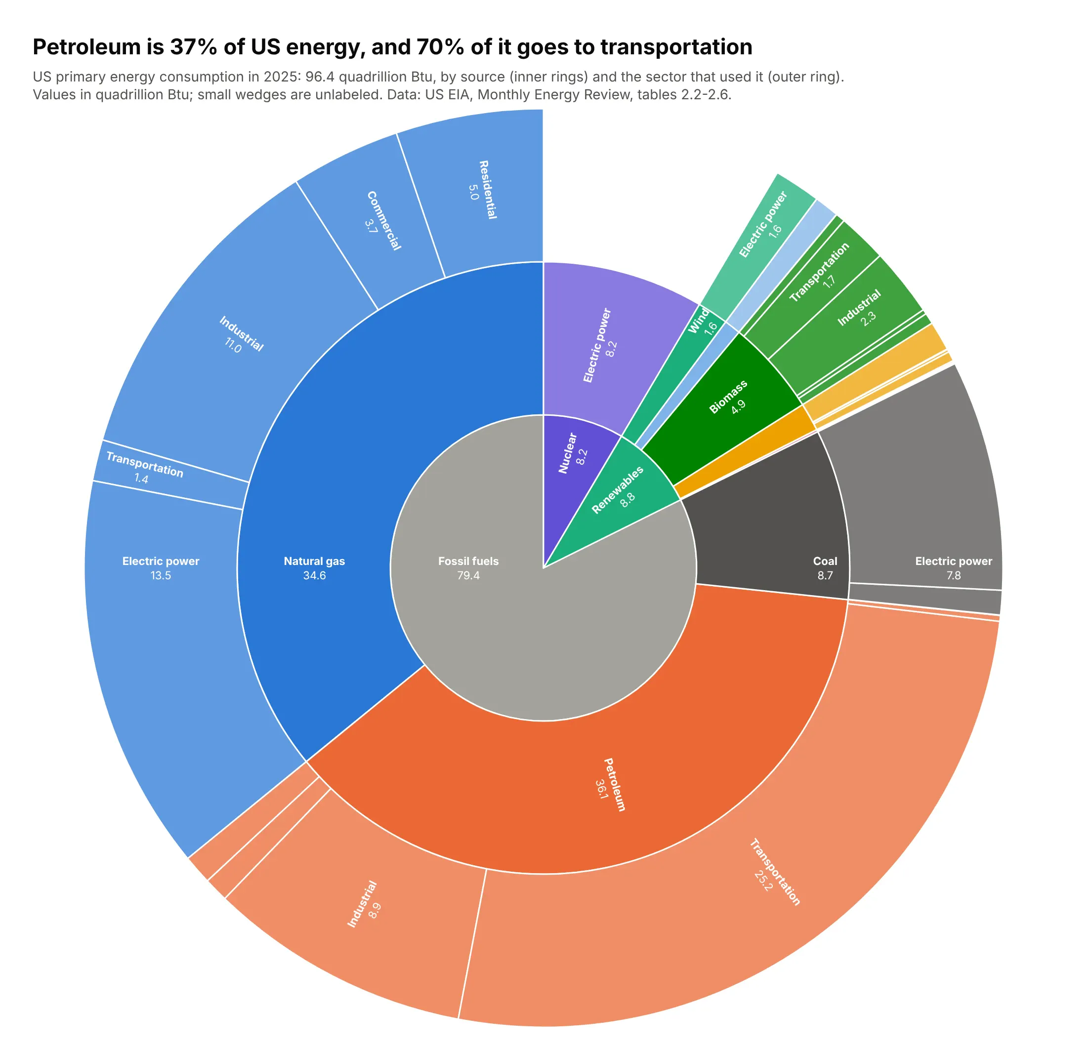
Data: US EIA, Monthly Energy Review, tables 2.2-2.6.

How do you read a sunburst chart? In the example above, notice these things:

• Start in the middle, where the inner ring splits all US primary energy into three fuel families. The gray fossil fuels wedge takes most of the circle, and nuclear and renewables are two thin slices at the top right.
• Each ring further out goes one level deeper, and a wedge's angle is its share of the total. Petroleum and natural gas fill most of the middle ring, while wind and solar are slivers inside renewables.
• A parent's children exactly fill its angle, so you can follow one source outwards. The orange petroleum wedge splits into the sectors that used it, and transportation takes about 70% of it.
• The outer wedges keep a lighter shade of their source's color, so they stay grouped by source and the same sector shows up in several places. Electric power appears under all nine sources, and comparing sectors means adding those wedges up yourself.
• Outer wedges cover more area than inner wedges with the same angle, which makes the outer ring look bigger than it is. Compare angles instead, and hover over the unlabeled slivers to read their values.

It's often used for charts like these:

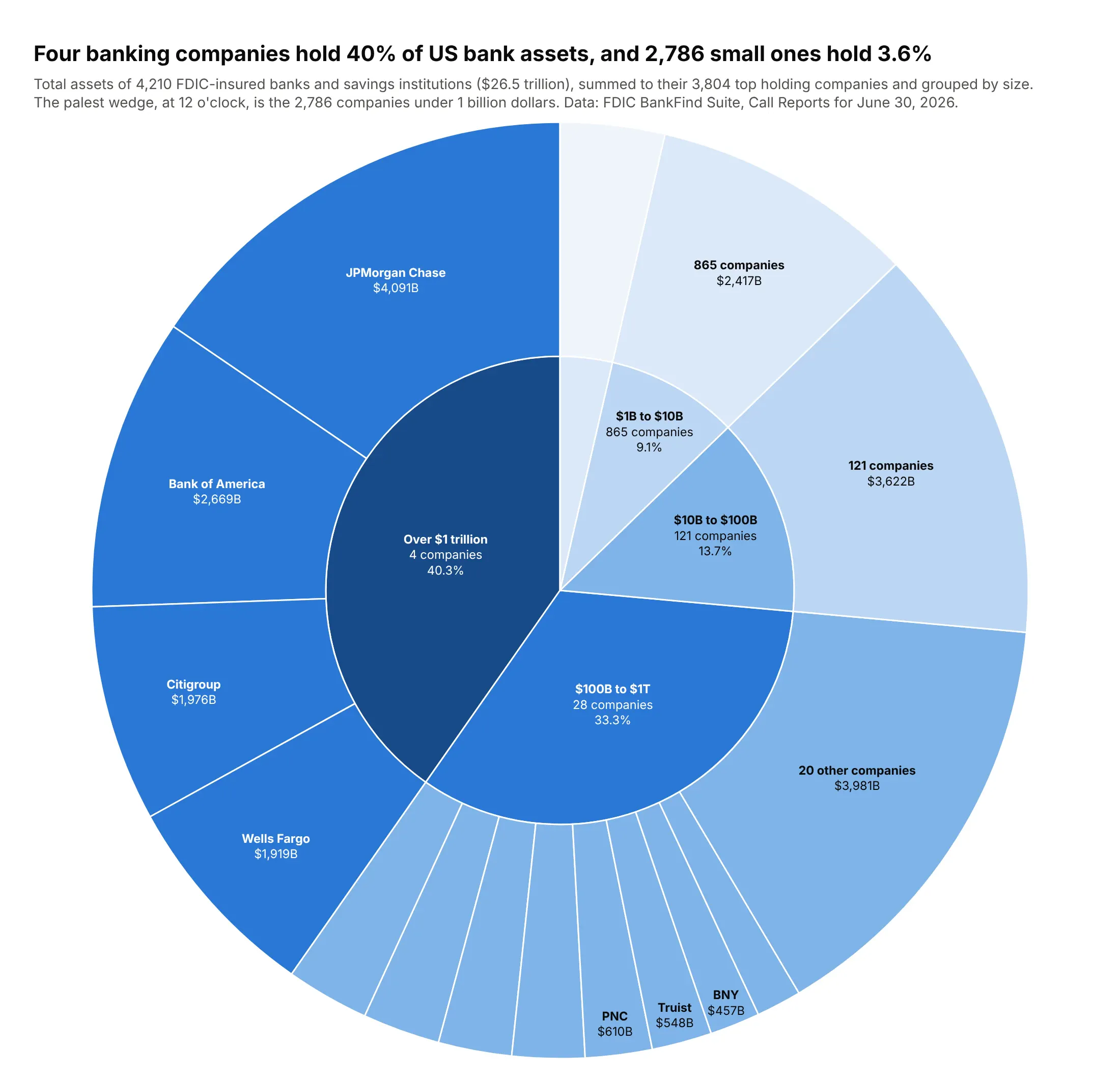
Who holds the money. The 4,210 FDIC-insured banks hold $26.5 trillion, and four companies (JPMorgan Chase, Bank of America, Citigroup and Wells Fargo) hold 40% of it, while 2,786 companies under $1 billion hold 3.6%. Data: FDIC BankFind Suite, June 30, 2026.

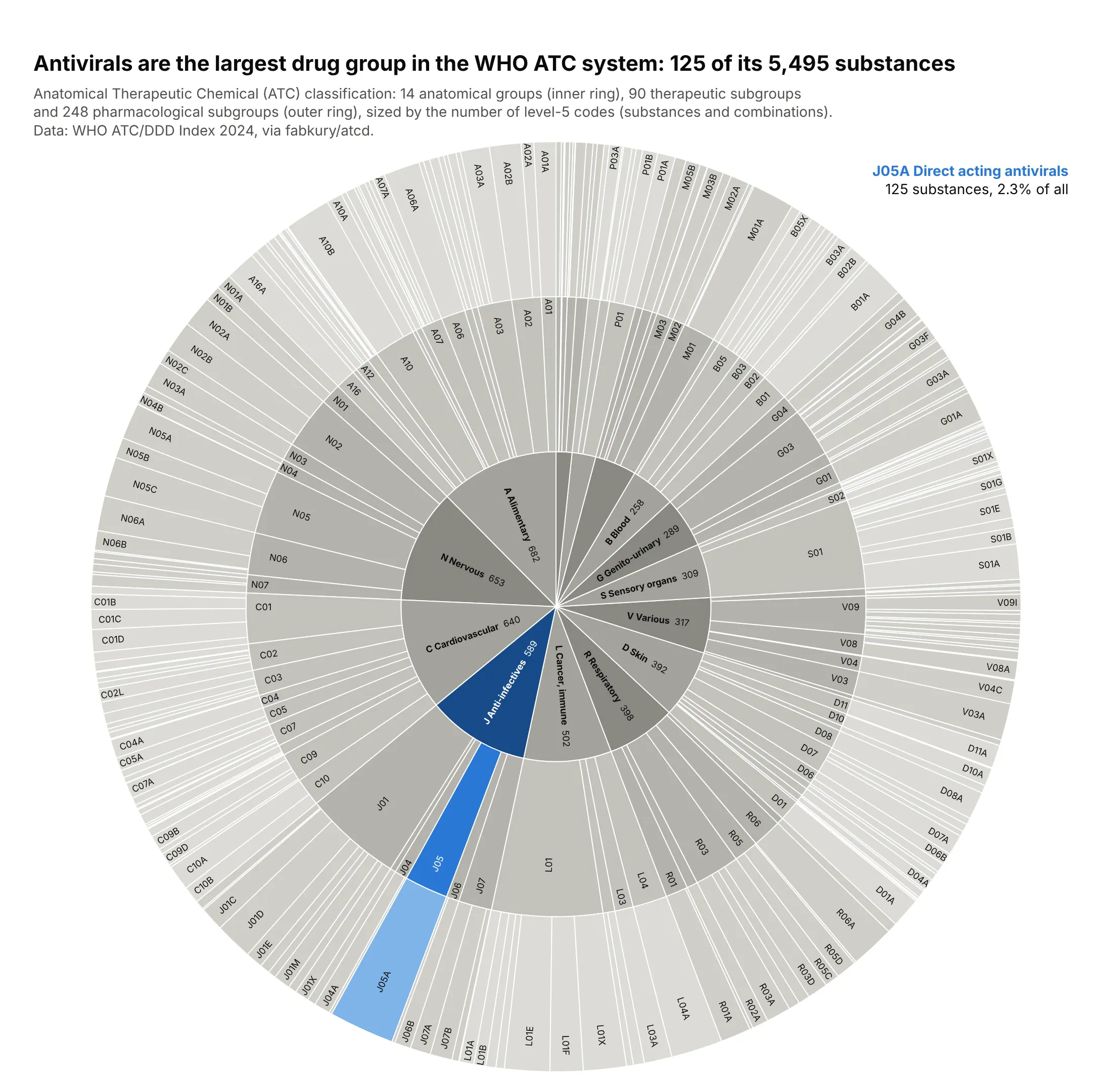
A taxonomy. The WHO Anatomical Therapeutic Chemical system sorts 5,495 drug substances into 14 anatomical groups, 90 therapeutic and 248 pharmacological subgroups, and the largest pharmacological group is J05A, direct acting antivirals, with 125 substances. Data: WHO ATC/DDD Index 2024, via fabkury/atcd.

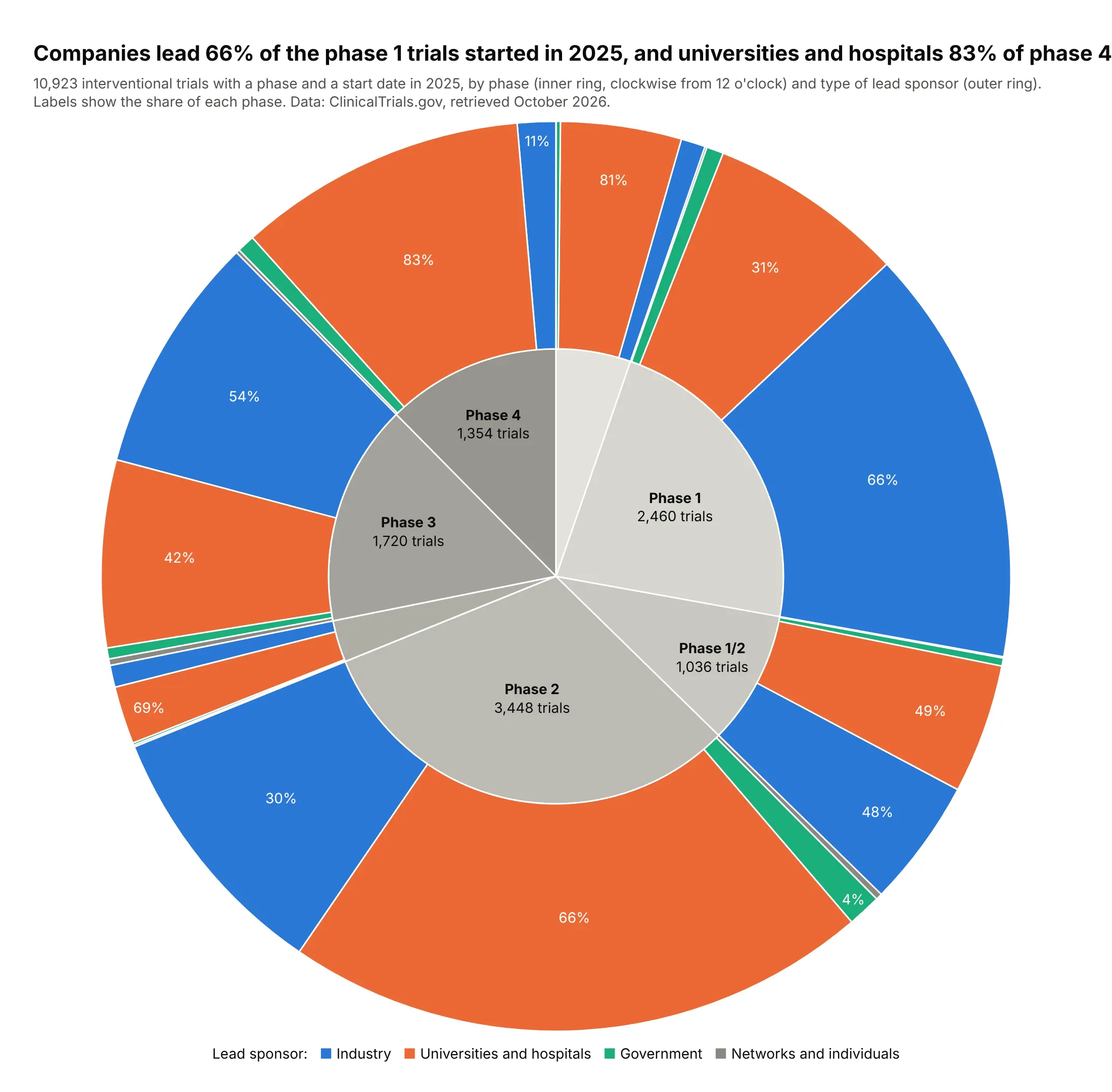
One category split by another. With the same sponsor colors under every phase, the outer ring shows that companies led 66% of the phase 1 trials started in 2025 and universities and hospitals led 83% of phase 4 trials. Data: ClinicalTrials.gov API, retrieved October 2026.

A short history

John Stasko's group at Georgia Tech built the Sunburst tool around 2000 to browse file systems, and Stasko and Eugene Zhang described it in a 2000 IEEE InfoVis paper; Keith Andrews and Helmut Heidegger ("Information Slices") and Mark Chuah had built similar radial layouts in 1998. In a study published the same year, people doing file and directory tasks preferred the sunburst to a treemap because it showed the structure of the hierarchy better. Here is that original idea, a directory tree as rings, redrawn with Plotly on the Linux source code:

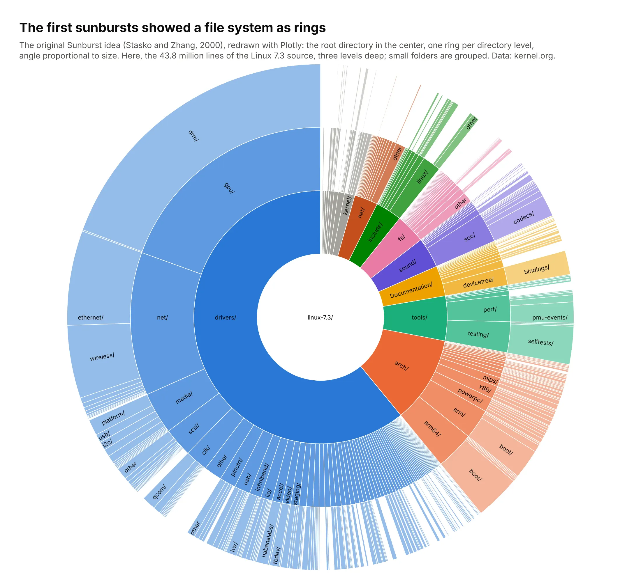
Disk usage tools such as Filelight and GNOME's Disk Usage Analyzer still draw ring charts for the same reason.

Alternatives to a sunburst chart

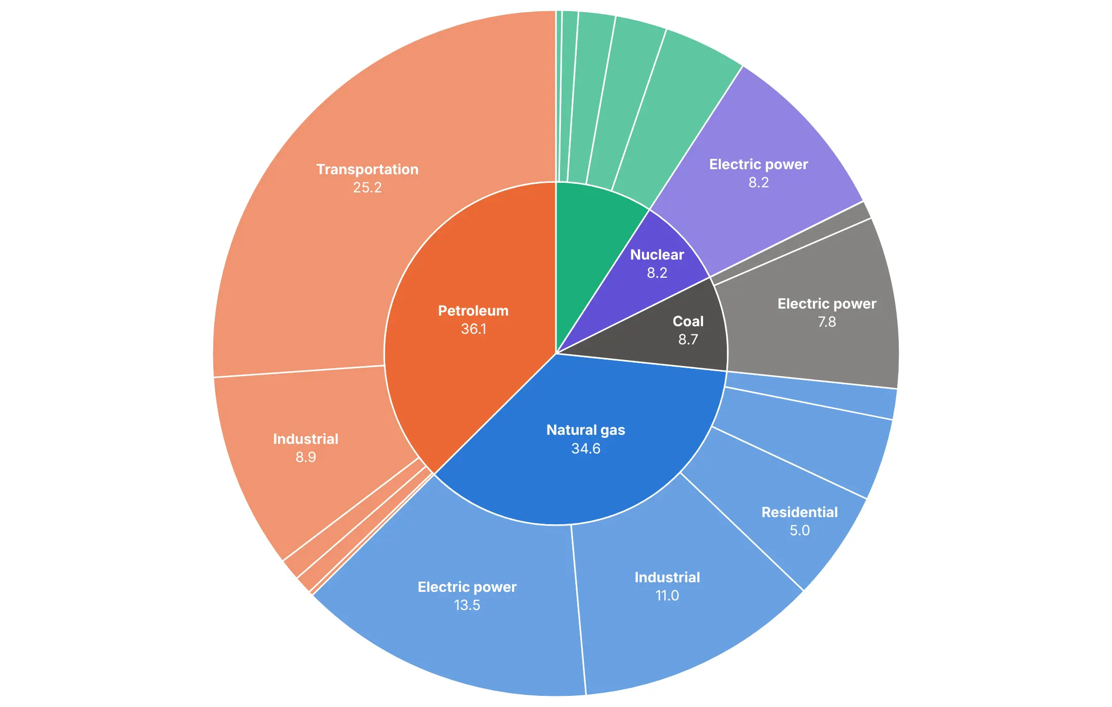
Here's the same US energy hierarchy drawn six ways. Some are better for the question, some worse, some just different:

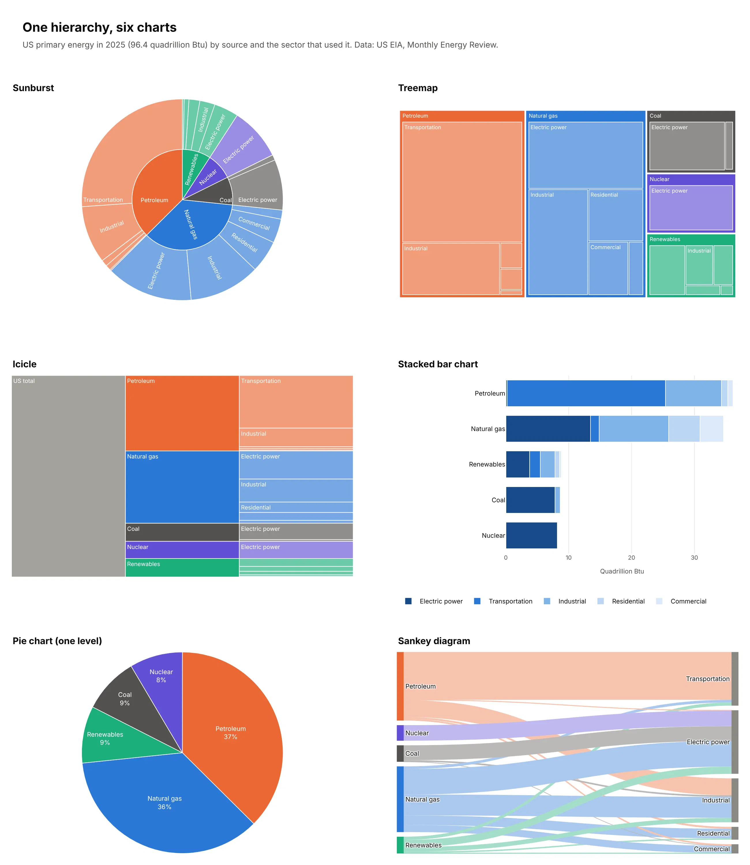
• Treemap (better for comparing sizes). Nested rectangles use every pixel and make sizes easier to compare, so they hold hundreds of items, but depth is only visible as nesting. People judge angles and curved areas less accurately than lengths and rectangles, as Cleveland and McGill (1984) measured. See our treemap guide.
• Icicle (different). The sunburst unrolled into columns, so depth reads left to right and outer levels don't get extra space for being further out. See our icicle chart guide.
• Stacked bar chart (better for precise comparisons, with two levels). Bars on a shared baseline show that natural gas (34.6 quads) is close to petroleum (36.1) more clearly than any of the radial charts, but a third level doesn't fit.
• Pie chart (works too, for one level). A sunburst with one ring is a pie chart, and for a single level the pie is simpler. Here petroleum is 37% of the total.
• Sankey diagram (different). Shows the same split as flows from sources to sectors, and also handles flows that merge, which a strict tree can't. See our Sankey diagram guide.

How to make a sunburst chart

With AI

ChatGPT, Claude Code, GitHub Copilot, Cursor and other AI tools are excellent at writing Plotly code. Name Plotly in the prompt, describe the levels and what color should mean, and list the checks you want:

With Plotly Studio

Plotly Studio is a desktop app where you point an AI at a dataset and it builds charts and a Dash app around your questions. Ask for a sunburst the same way:

Show a sunburst of NHS prescription costs by BNF chapter, section and drug. Color by chapter, fold drugs under 2% of their section into "Other", put the cost on every wedge and hide labels that don't fit. Add a dropdown to size by cost or by number of items.

Make a sunburst chart in Python or JavaScript

This is the code AI tools write under the hood. In Python, Plotly Express builds the hierarchy from a flat table with one column per level, and px.Constant adds a root:

In JavaScript, plotly.js takes one entry per wedge with its label, its parent and its value:

Ids must be unique, which is why both "Industry" wedges get an id built from their path. With branchvalues="total", each parent's value must equal the sum of its children, or Plotly draws an empty chart without an error.

Share it

Every Plotly chart has a Share chart button (the cloud icon in its toolbar) that uploads it to Plotly Cloud and gives you a link. Only you can see it until you change its visibility.

For a live app, put the chart in a Dash app and publish it with the Plotly Cloud CLI. In a Dash app, clicking a wedge zooms into it, and the clickData of the dcc.Graph tells your callback which wedge was clicked, so the sunburst can filter a table or another chart. Coding agents can run these commands for you:

If your data has to stay in your own cloud or data center, publish to Dash Enterprise instead.

Dos and don'ts

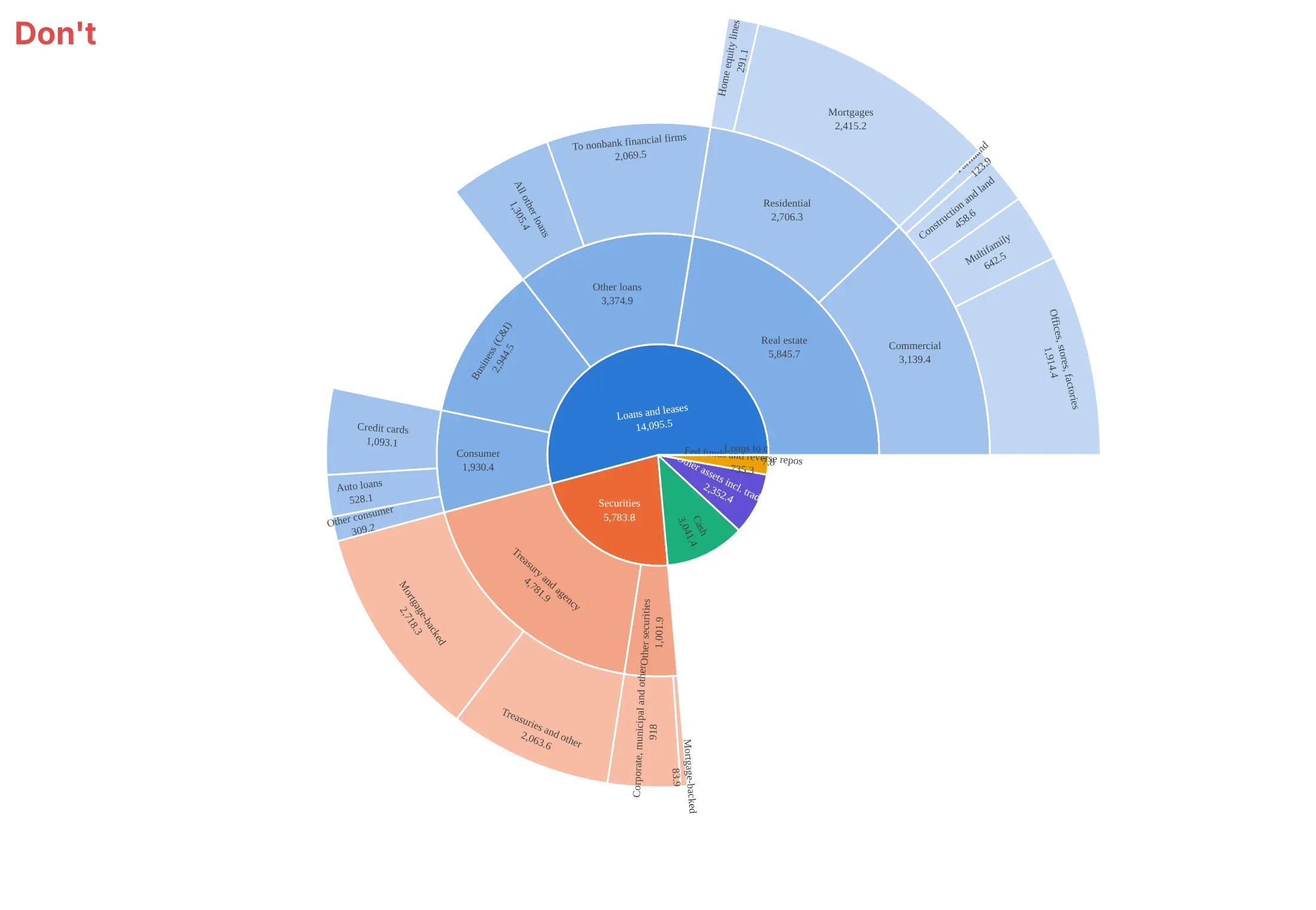
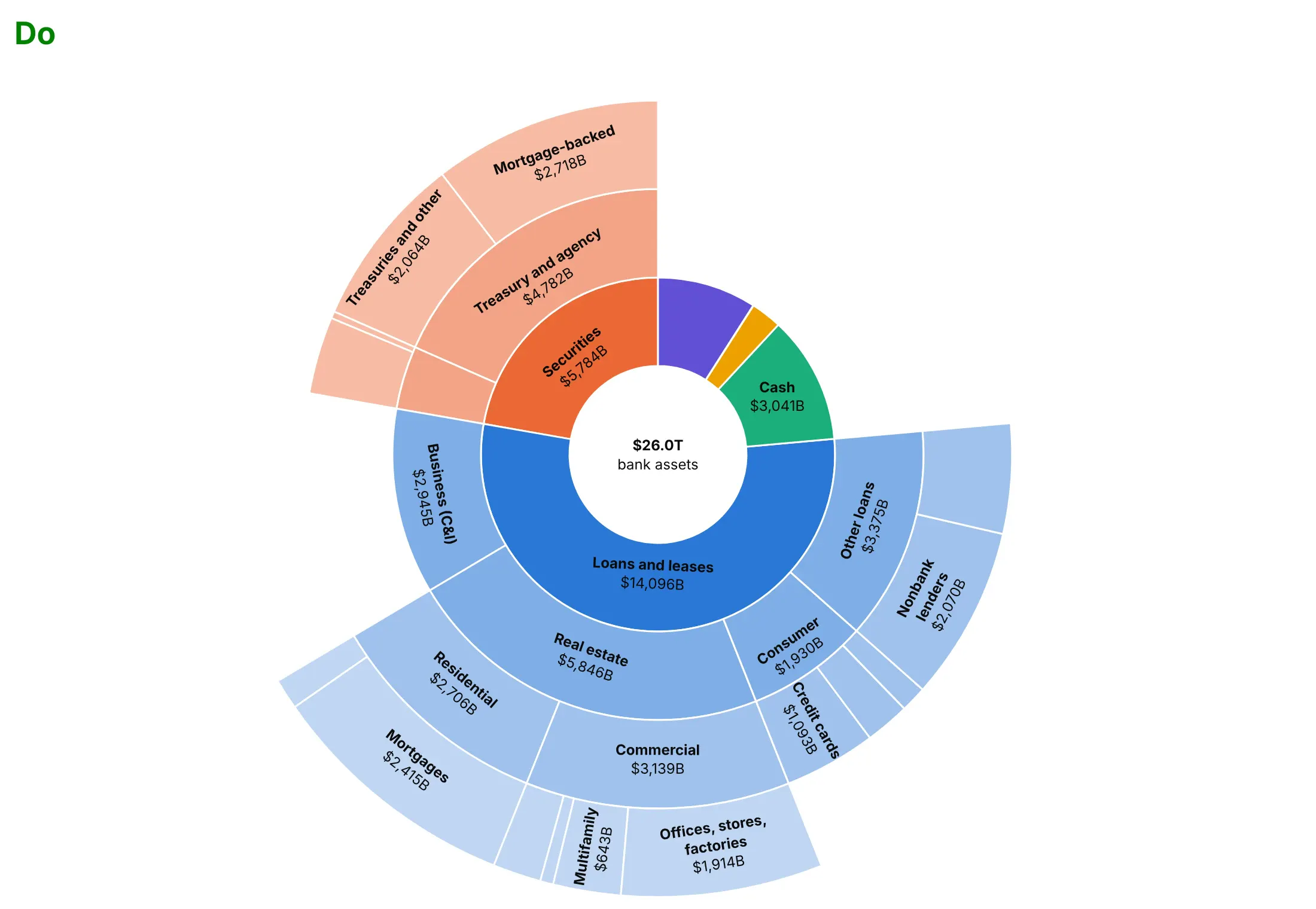
Plotly's defaults are made for exploring. For a published chart, most of the work is deciding what to leave out. Here are the assets of US commercial banks in September 2026, $26.0 trillion, both ways.

Don't print raw unformatted numbers, force a label into every wedge or leave the center empty:

Do use the same colors, but format the values as dollars, hide labels that don't fit and put the total in the center:

Use color for one other thing

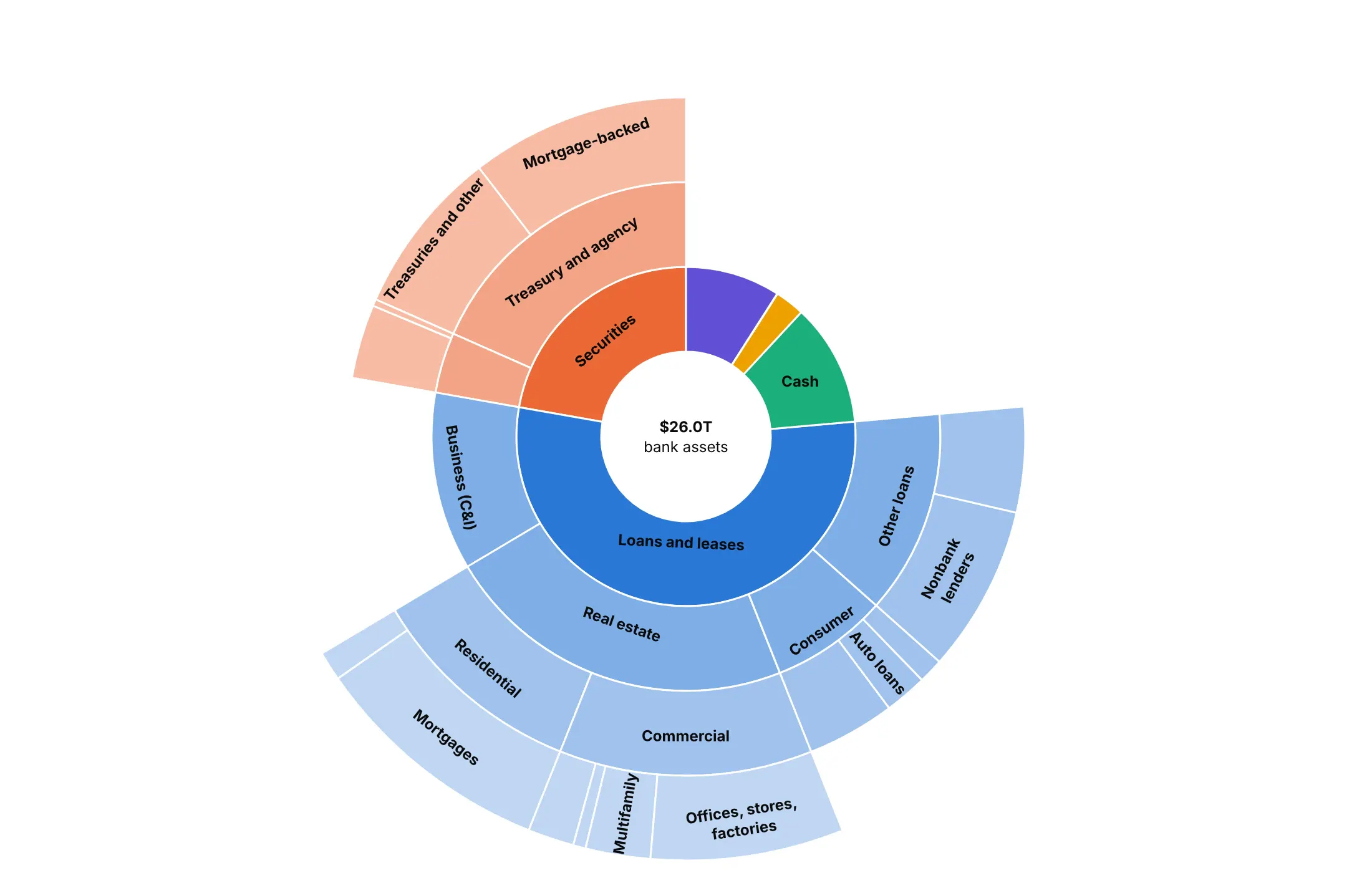
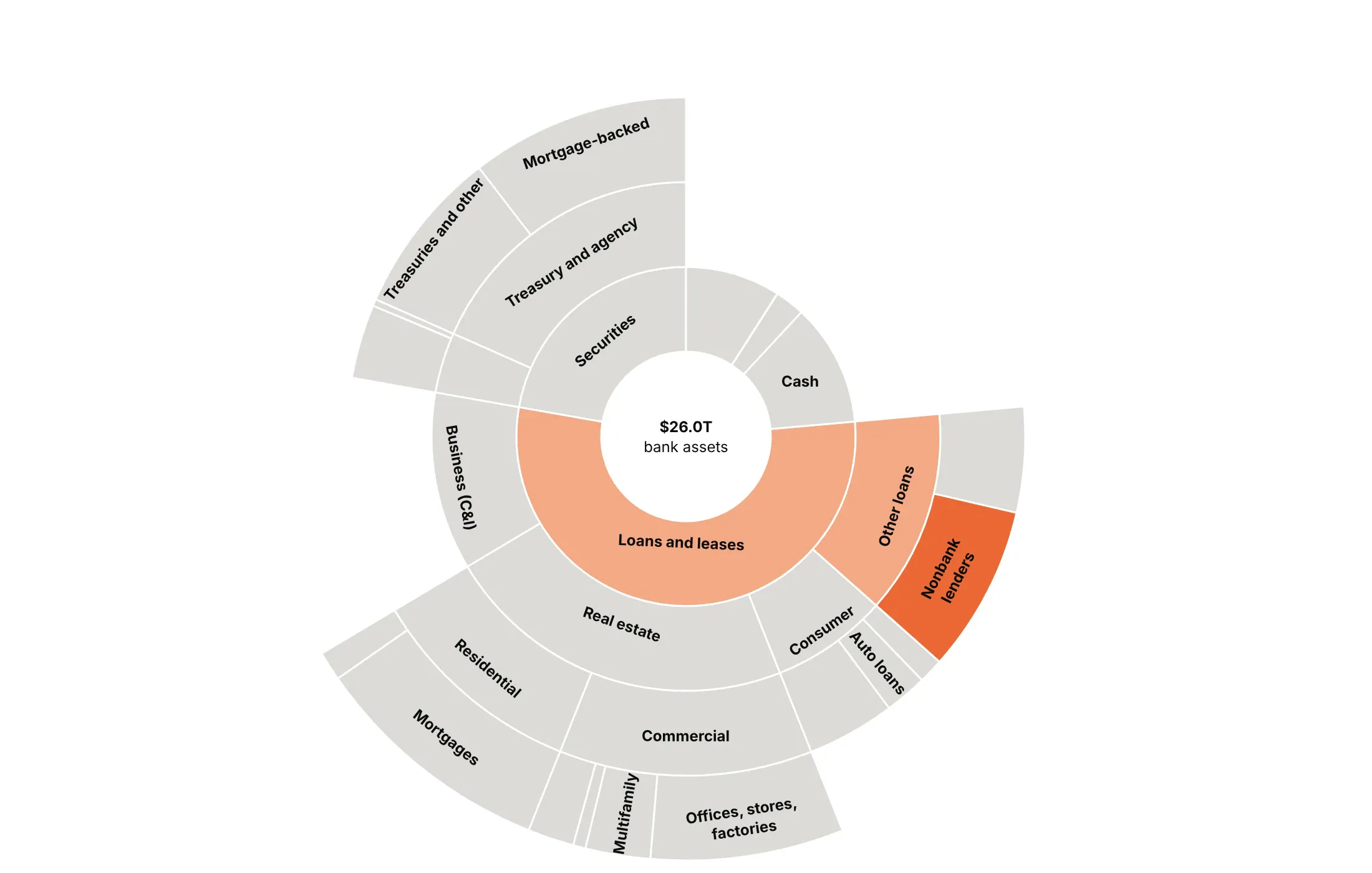
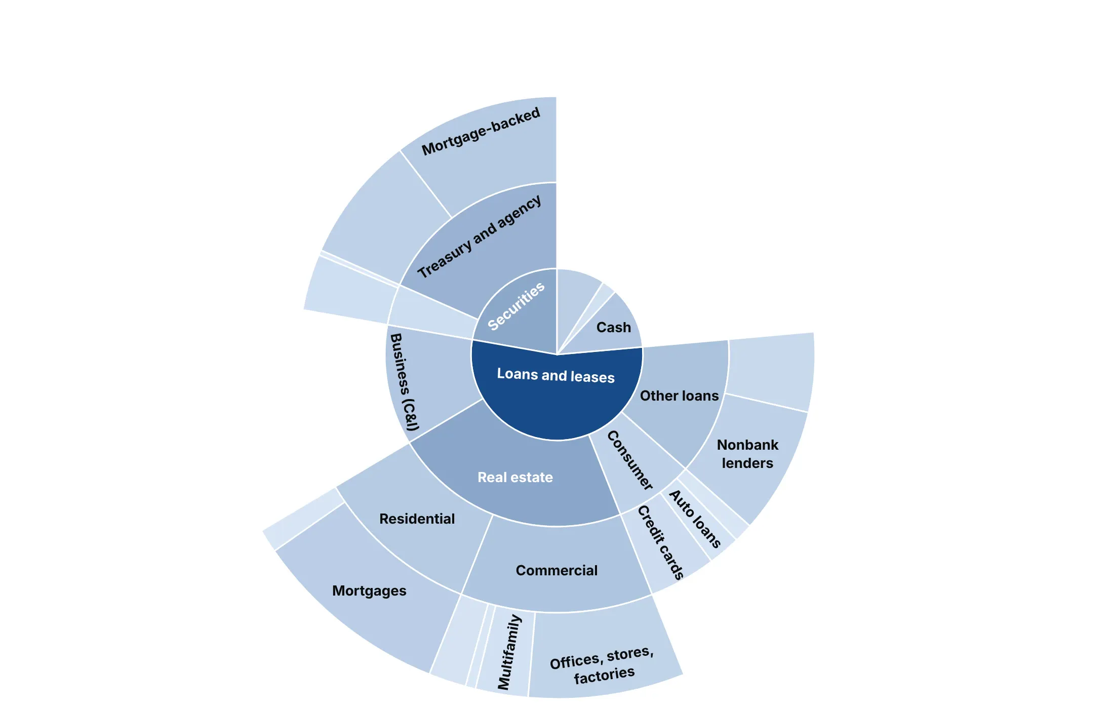
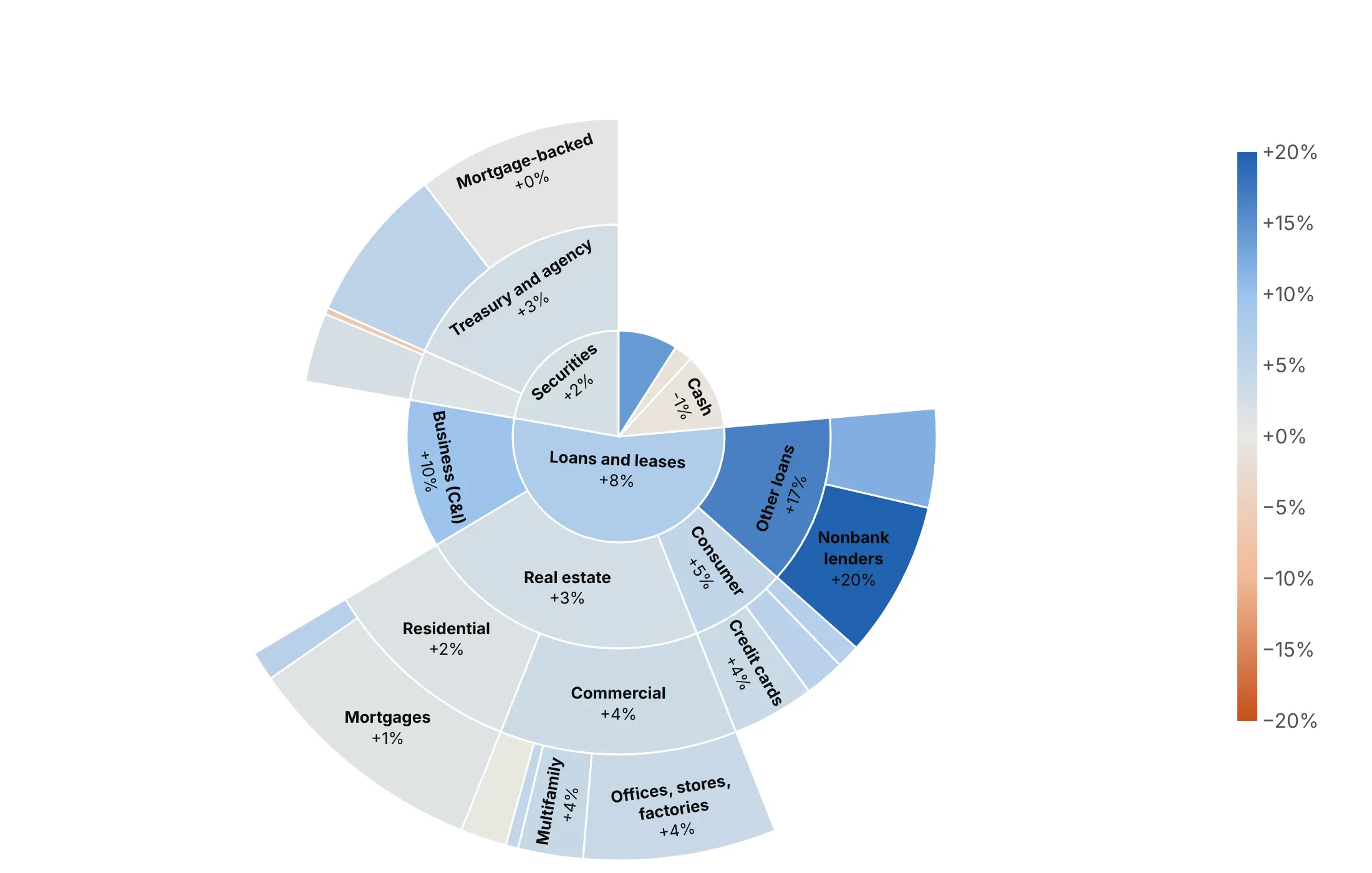
Angle already shows size, so color is free to say something else. Here are four options on the same balance sheet.

By group. Shows the structure, and it's a good default when the top-level groups matter.

Highlight one story. Loans to nonbank financial firms grew fastest, so only their path is in color and everything else is gray.

By size (avoid). Color repeats what the angle already shows, so it adds nothing.

By a second variable. Here it's the change since September 2025: loans to nonbank lenders (+20%) are the darkest blue, and cash (-0.9%) is close to gray.

Fit the labels to the wedges

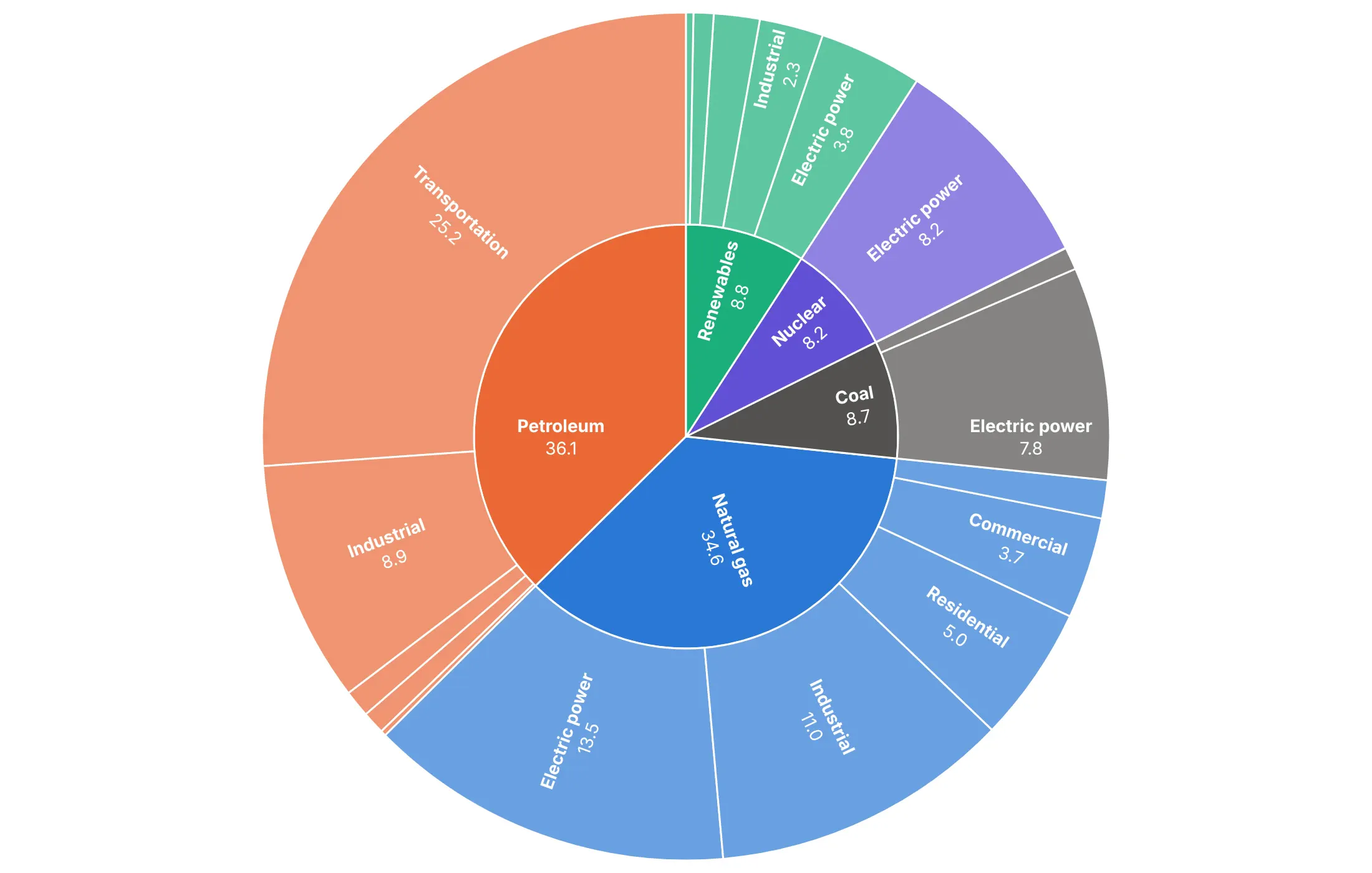
insidetextorientation controls how text sits in a wedge. horizontal is the easiest to read when the wedges are big enough:

radial runs the text along the radius, so thin outer wedges keep their labels:

Checklist

Do

• Write a title that states the takeaway, such as "Petroleum is 37% of US energy, and 70% of it goes to transportation".
• Put numbers on the wedges with texttemplate, using %{percentRoot} for the share of the total or %{percentParent} for the share within a branch.
• Hide labels that don't fit with uniformtext=dict(minsize=10, mode="hide").
• Control the order with sort=False and start at 12 o'clock with rotation=90. Wedges run counterclockwise, so pass ordered categories (years, phases) in reverse to read clockwise.
• Set leaf.opacity=1 when you chose the colors yourself, because the default fades the leaves.
• Use the center for the total by adding an explicit root node.
• Fold the long tail into "Other" wedges and keep two or three rings in static images.

Don't

• Color by size, because the angle already shows it.
• Use more than about eight hues. Color the top-level groups or one story, and gray the rest.
• Show every level of a deep tree in a static image; use maxdepth.
• Use a sunburst for one level. That's a pie chart, and bars are more precise.
• Rely on hover in a static image. Print the numbers that matter.

Options to customize

These are the go.Sunburst (and px.sunburst) options that matter most. The full list is in the Plotly sunburst documentation.

1. path (px only): builds the tree from DataFrame columns, top level first.
2. ids, labels, parents: the tree, one row per wedge. Ids must be unique, so build them from the path when labels repeat.
3. values: the size of each wedge.
4. branchvalues: total (a parent's value is the sum of its children) or remainder (added on top).
5. marker.colors: one color per wedge, for groups or a highlight.
6. marker.colorscale, cmid, cmin, cmax: map a number to color; cmid centers a diverging scale.
7. marker.line: wedge borders, usually thin white lines.
8. marker.pattern: hatching for a second category; set pattern.bgcolor too, or hatched wedges are transparent.
9. leaf.opacity: opacity of the outermost wedges (0.7 by default); set it to 1 when you pick the colors.
10. insidetextorientation: auto, horizontal, radial or tangential; radial suits thin outer wedges.
11. texttemplate: wedge text with %{label}, %{value}, %{percentRoot}, %{percentParent}, %{percentEntry}.
12. uniformtext (layout): a minimum font size; mode="hide" drops text that won't fit.
13. maxdepth, level: how many rings to show, and which wedge to start from.
14. rotation: the angle of the first wedge; 90 starts at 12 o'clock.
15. sort: set to False to keep your own order.
16. root.color: the color of the center; white or the background color makes a hole.
17. count: size by the number of leaves or branches when there's no value column.
18. hovertemplate, customdata: hover content, such as growth rates.
19. domain: place several sunbursts side by side.

More sunburst examples

Ten more sunbursts built from real public data, each with its source, the technique that makes it work and a prompt to rebuild it.

1. The power plants being planned in the US

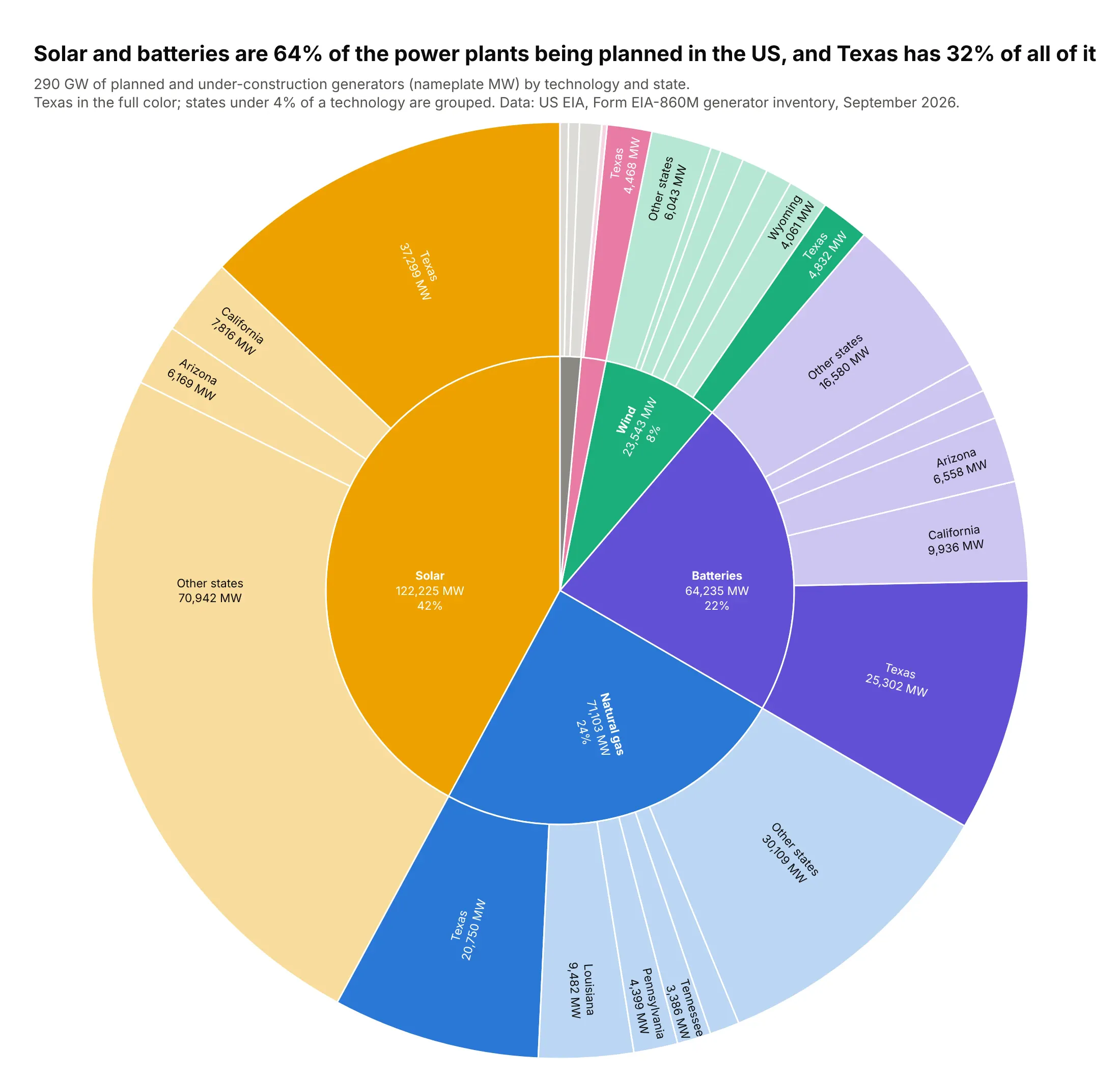
EIA's inventory lists 290 GW of generators planned or under construction. Solar and batteries are 64% of it, and Texas alone has 32%, including 37 GW of solar and 25 GW of batteries. Data: US EIA, Form EIA-860M, September 2026.

Tip: highlight one entity that appears under every parent (Texas) in the full hue and tint the rest, so the reader can add it up around the ring.

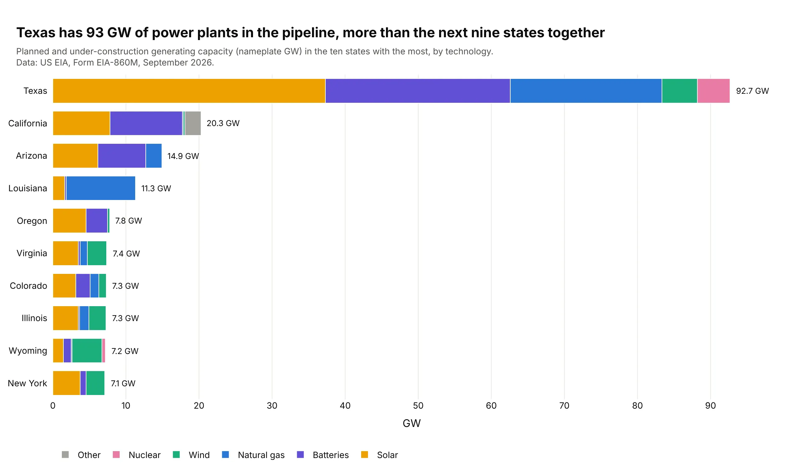
Another way to see it: a stacked bar per state ranks the states exactly. Texas's 92.7 GW is more than the next nine states together.

2. Where US crude oil comes from

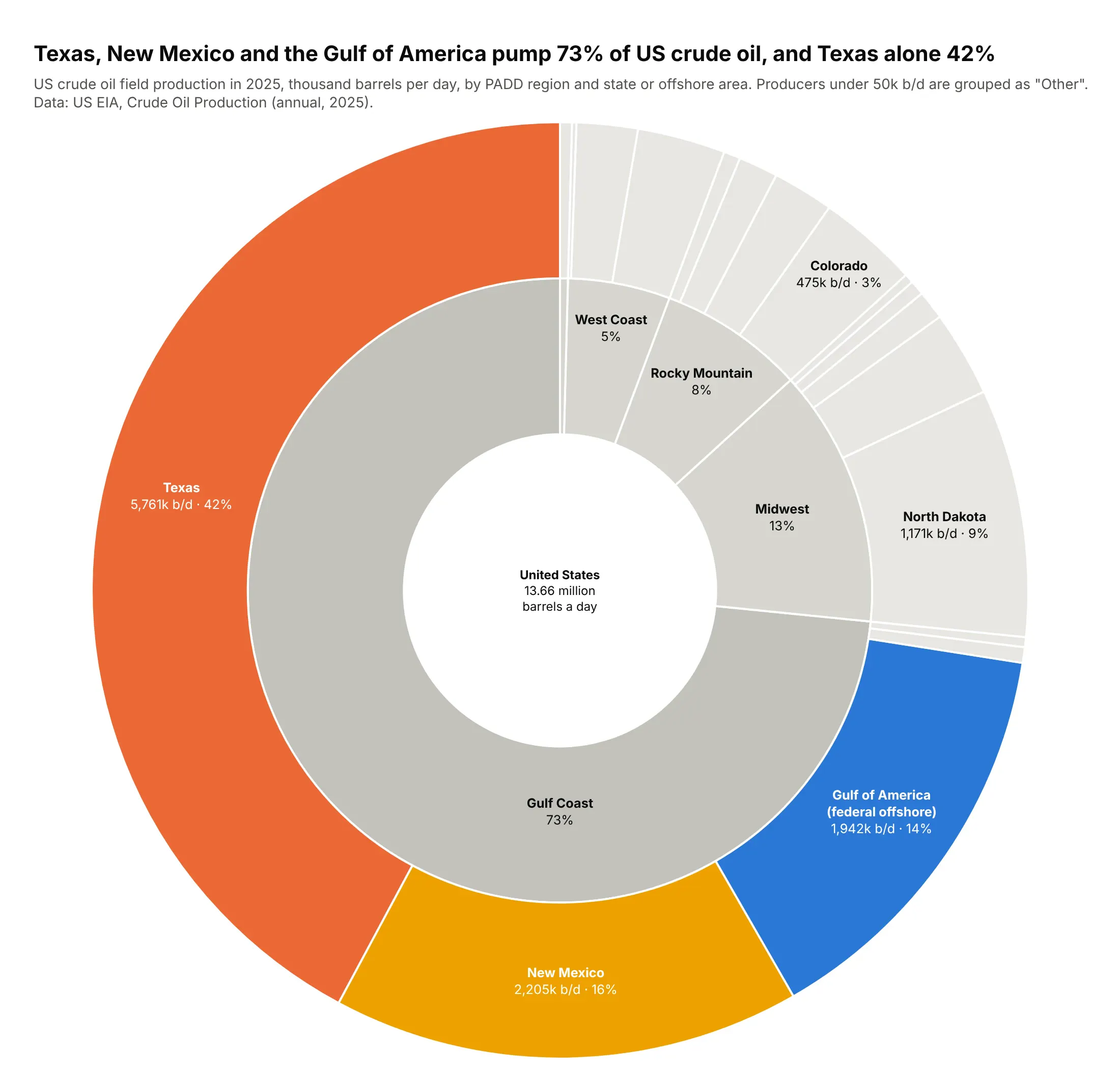
The US produced 13.66 million barrels a day in 2025, and the Gulf Coast region produced 73% of it. Three producers did most of the work: Texas (42%), New Mexico (16%) and federal offshore Gulf of America (14%). Data: US EIA, Crude Oil Production, annual 2025.

Tip: add an explicit root node drawn in white and put the total in its label, so the center carries the headline number.

3. What happened to every well drilled in the Gulf

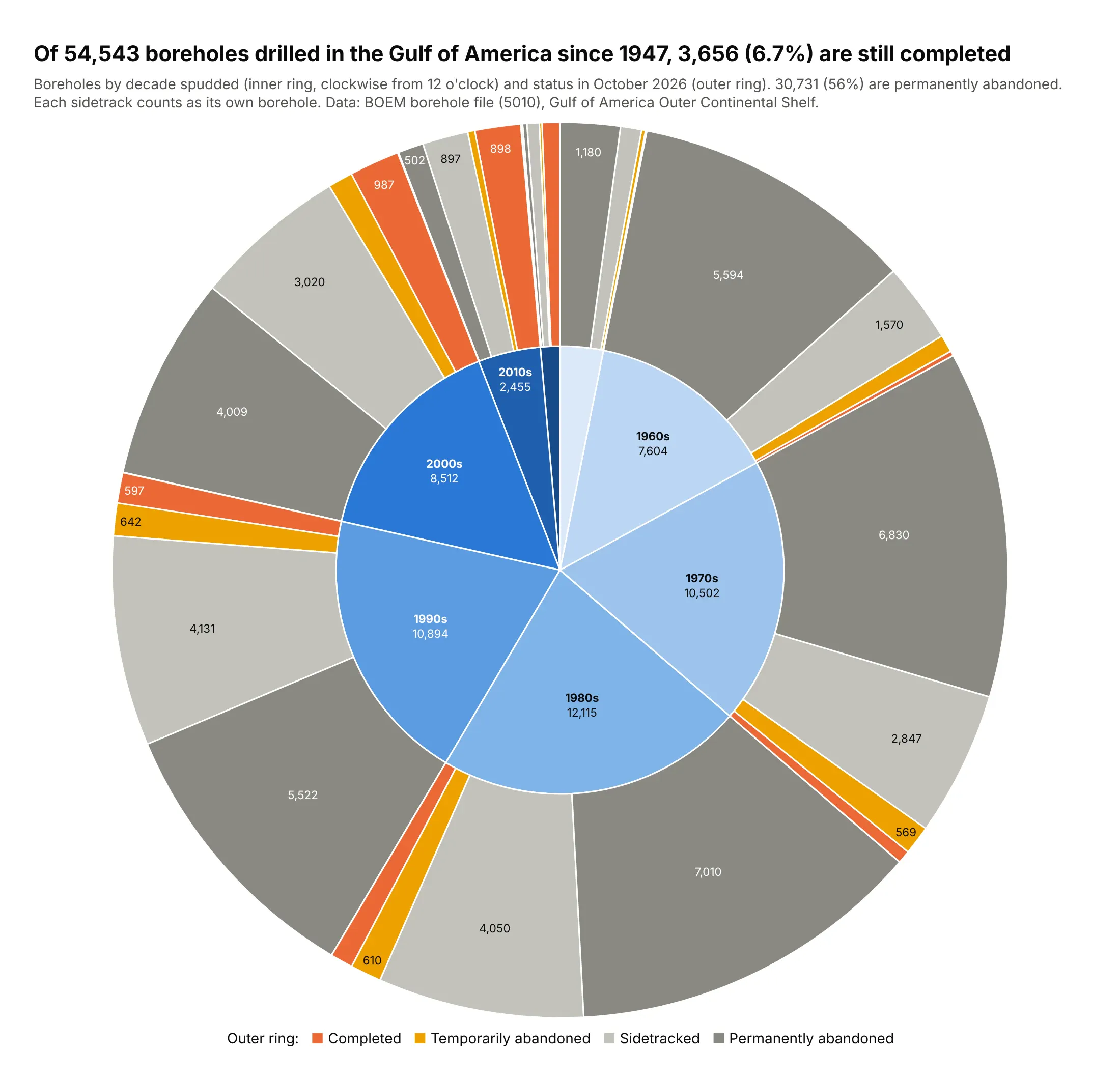
BOEM lists 54,543 boreholes drilled on the federal Gulf shelf and slope since 1947, with the peak in the 1980s (12,115). Only 3,656 (6.7%) are still completed, and 56% are permanently abandoned. Data: BOEM borehole file (5010), October 2026.

Tip: a ring read clockwise is a timeline. Use sort=False, rotation=90 and pass the decades newest first, because wedges run counterclockwise.

4. Where the world's greenhouse gases come from

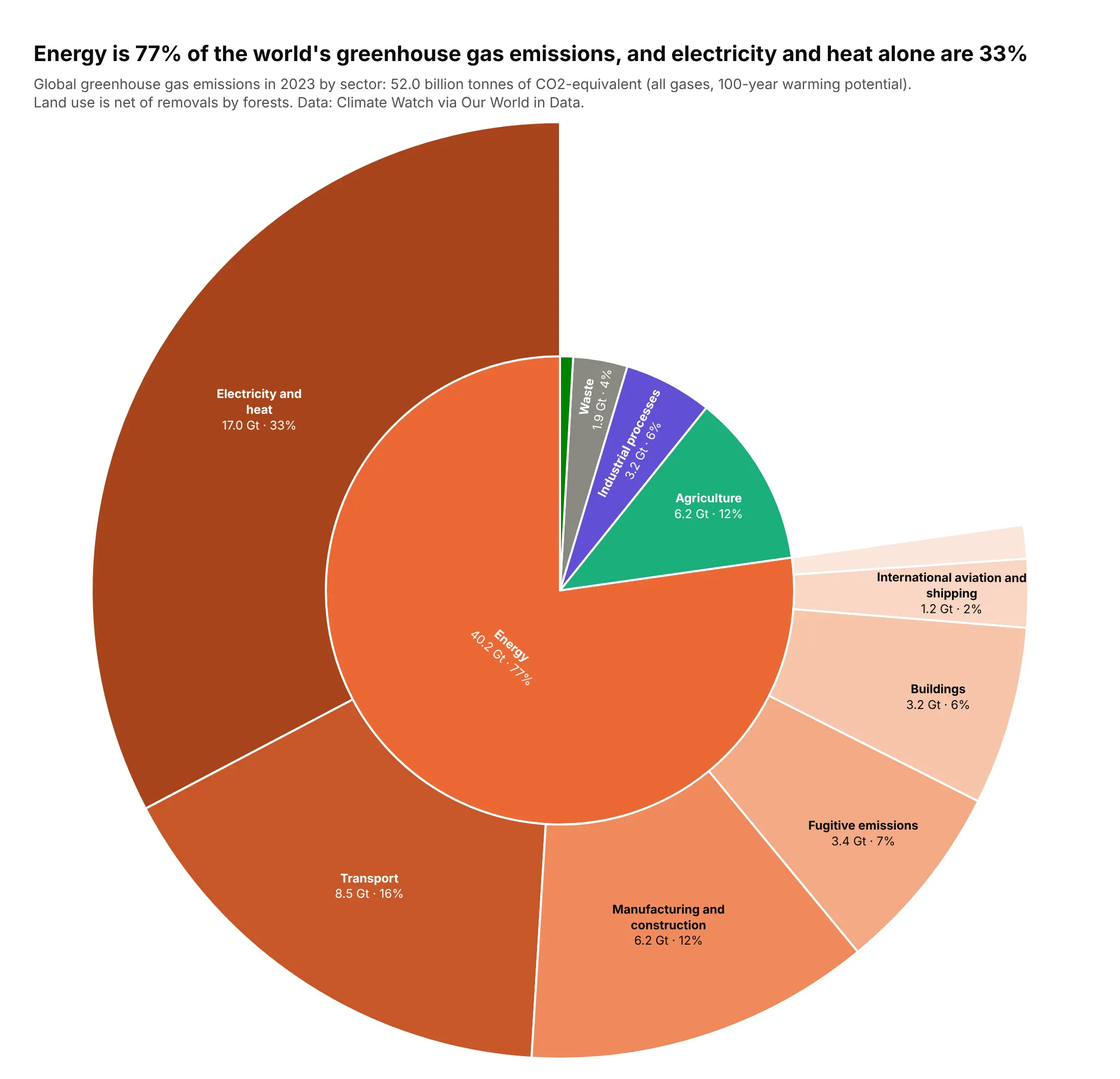
The world emitted 52.0 billion tonnes of CO2-equivalent in 2023. Energy was 77% of it, and electricity and heat alone 33%. Agriculture (12%) is the largest sector outside energy. Data: Climate Watch via Our World in Data, 2023.

Tip: a ragged tree is fine: only energy has children, so the other sectors stay single wedges and the extra ring shows where the detail is.

5. What Norway's oil fund owns

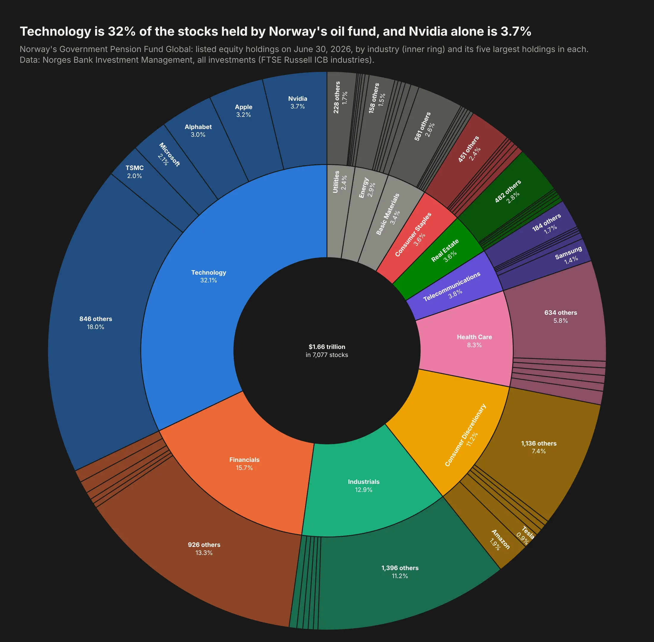
Norway's Government Pension Fund Global held $1.66 trillion of stocks in 7,077 companies in June 2026. Technology is 32% of it, and Nvidia alone is 3.7%, followed by Apple and Alphabet. Data: Norges Bank Investment Management, all investments, June 30, 2026.

Tip: on a dark background, let companies inherit their industry's hue at leaf.opacity=0.55 and leave the center as a hole that holds the total.

6. New York City's budget

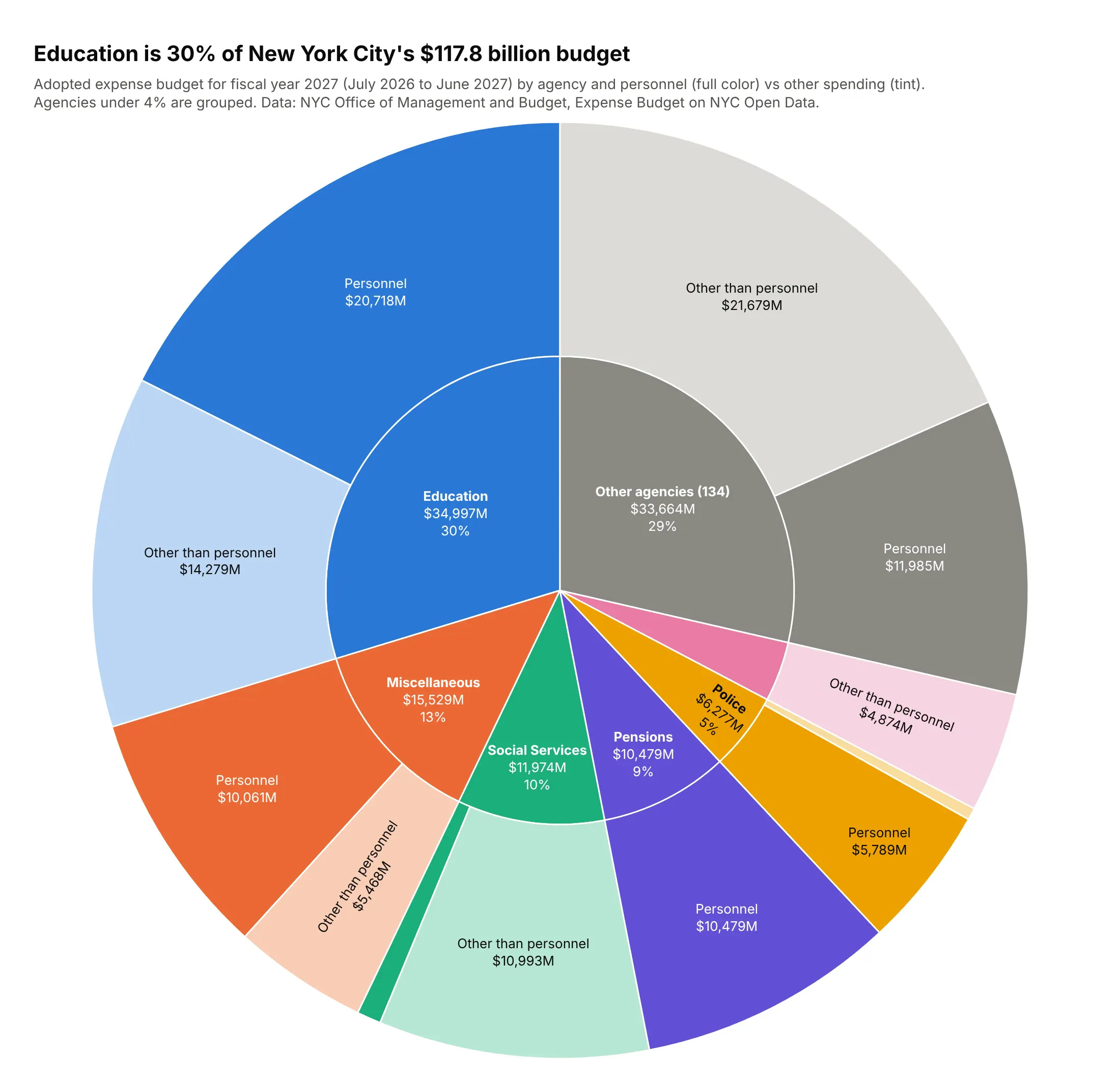
New York City adopted a $117.8 billion budget for fiscal 2027. Education is 30% of it ($35.0 billion), followed by citywide "miscellaneous" costs, mostly fringe benefits (13%), and social services (10%). Data: NYC Office of Management and Budget, Expense Budget on NYC Open Data.

Tip: maxdepth=2 keeps the static chart to two rings while the HTML version holds a third level (object class) for drill-down.

7. What the NHS pays for prescriptions

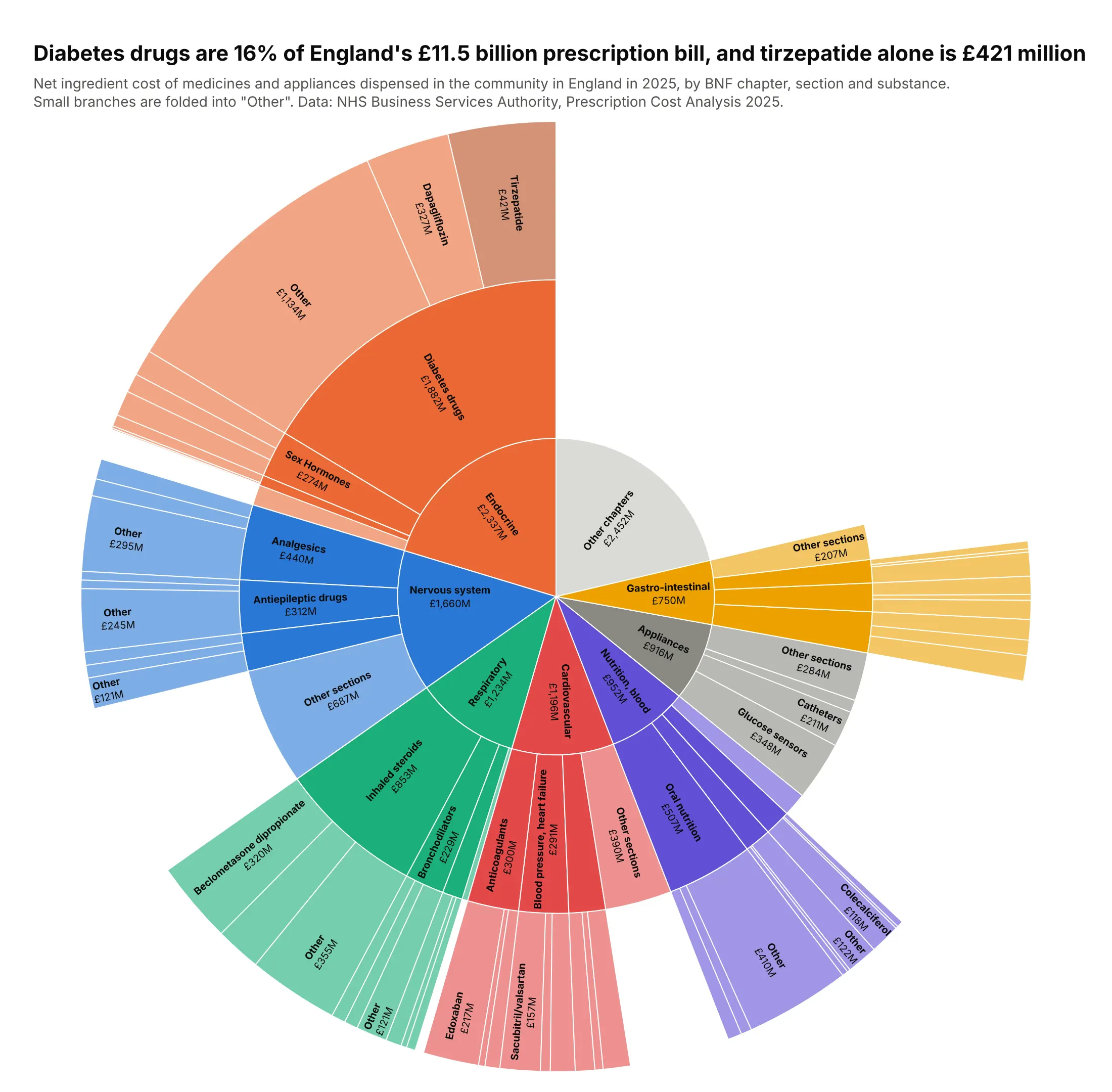
Medicines dispensed in the community in England cost £11.5 billion in 2025. Diabetes drugs were 16% of it, and tirzepatide (Mounjaro) was the most expensive single drug at £421 million, ahead of glucose sensors and dapagliflozin. Data: NHS Business Services Authority, Prescription Cost Analysis 2025.

Tip: three rings answer three questions (chapter, section, drug); fold the tail at each level so the outer ring stays readable.

8. Who pays for US health care

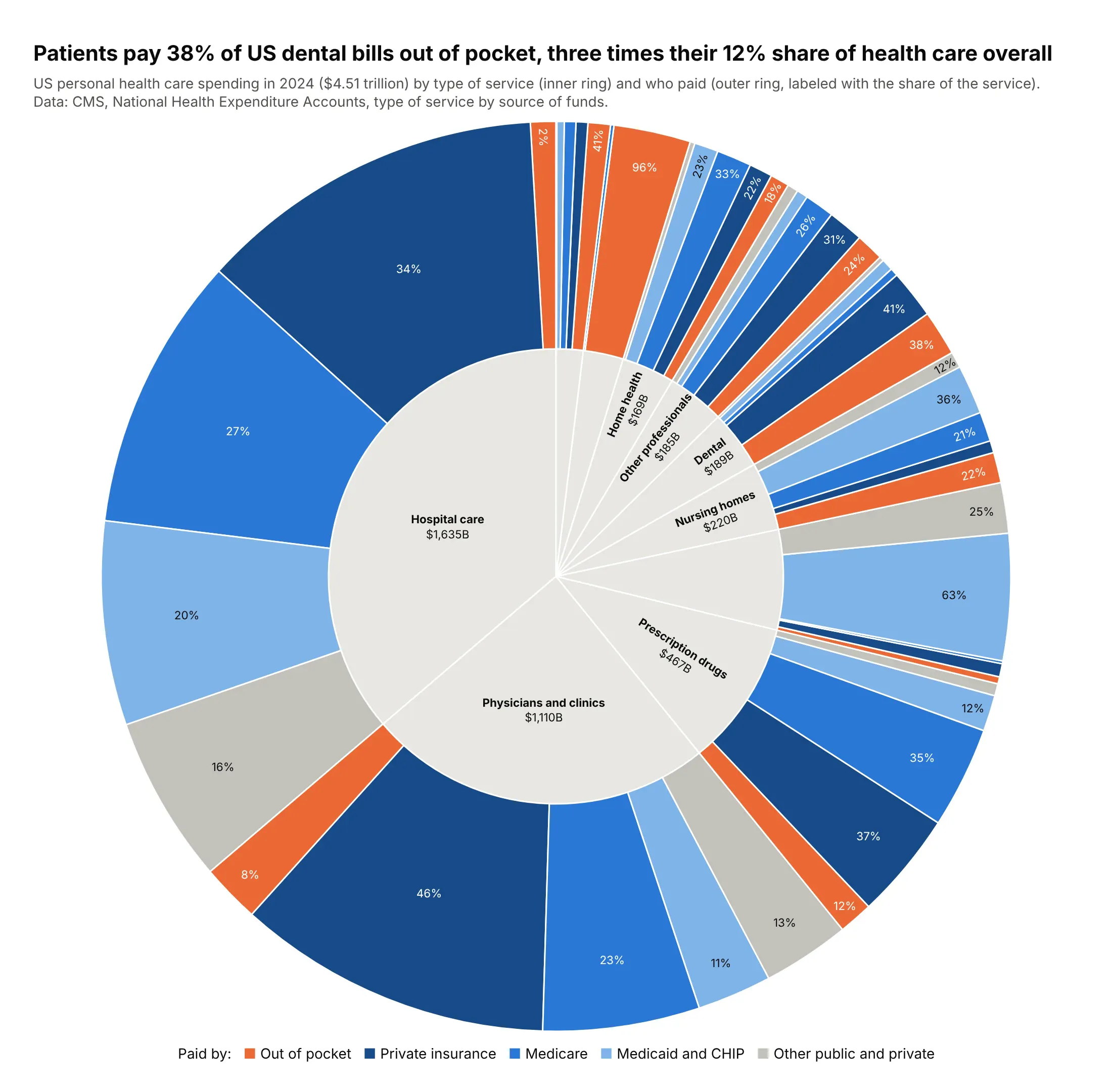
Americans spent $4.51 trillion on personal health care in 2024, and patients paid 12% out of pocket. For dental care the share is 38%, three times as much, while for hospital care it is 2.5%. Data: CMS, National Health Expenditure Accounts, 2024.

Tip: the same five payer colors under every service turn the outer ring into ten small distributions you can compare.

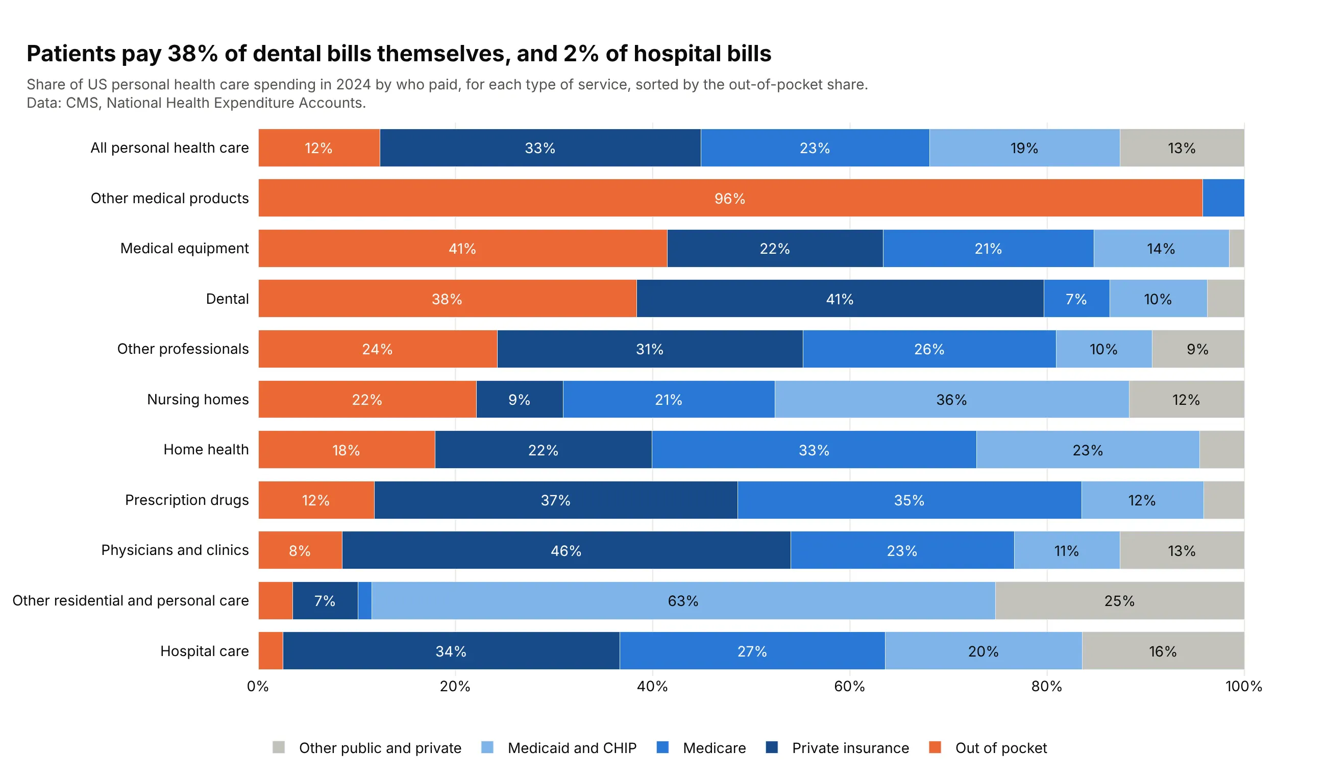
Another way to see it: 100% stacked bars sorted by the out-of-pocket share show that other medical products (96%) and medical equipment (41%) rank above dental.

9. Where the code is in the Linux kernel

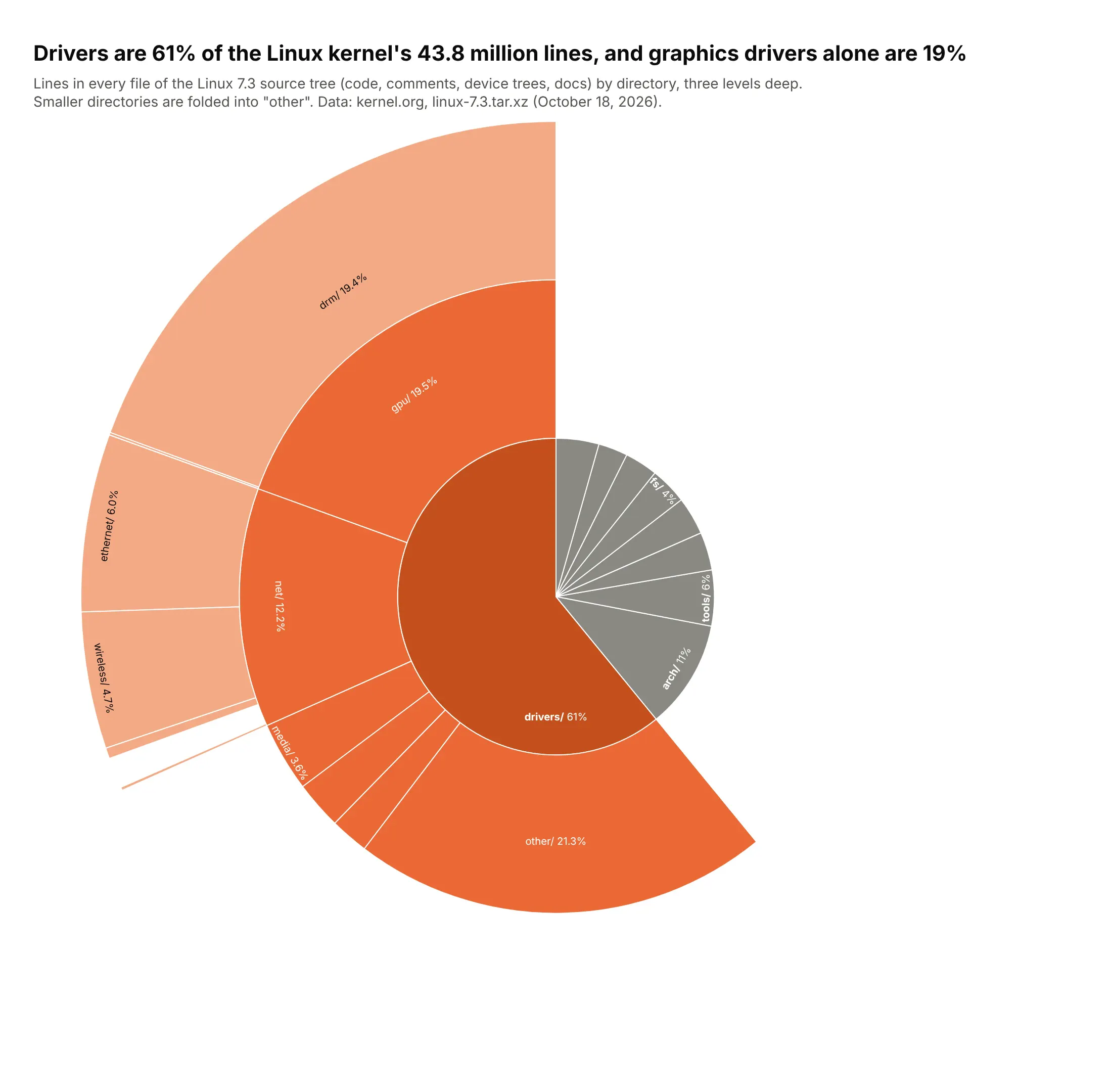
Linux 7.3 has 95,978 files and 43.8 million lines. Drivers are 61% of them, and graphics drivers alone are 19%, more than the whole arch/ directory (11%). Data: kernel.org, linux-7.3.tar.xz, October 18, 2026.

Tip: open only the branch that carries the story and leave every other directory as one gray wedge.

10. Formula 1 wins by team and driver

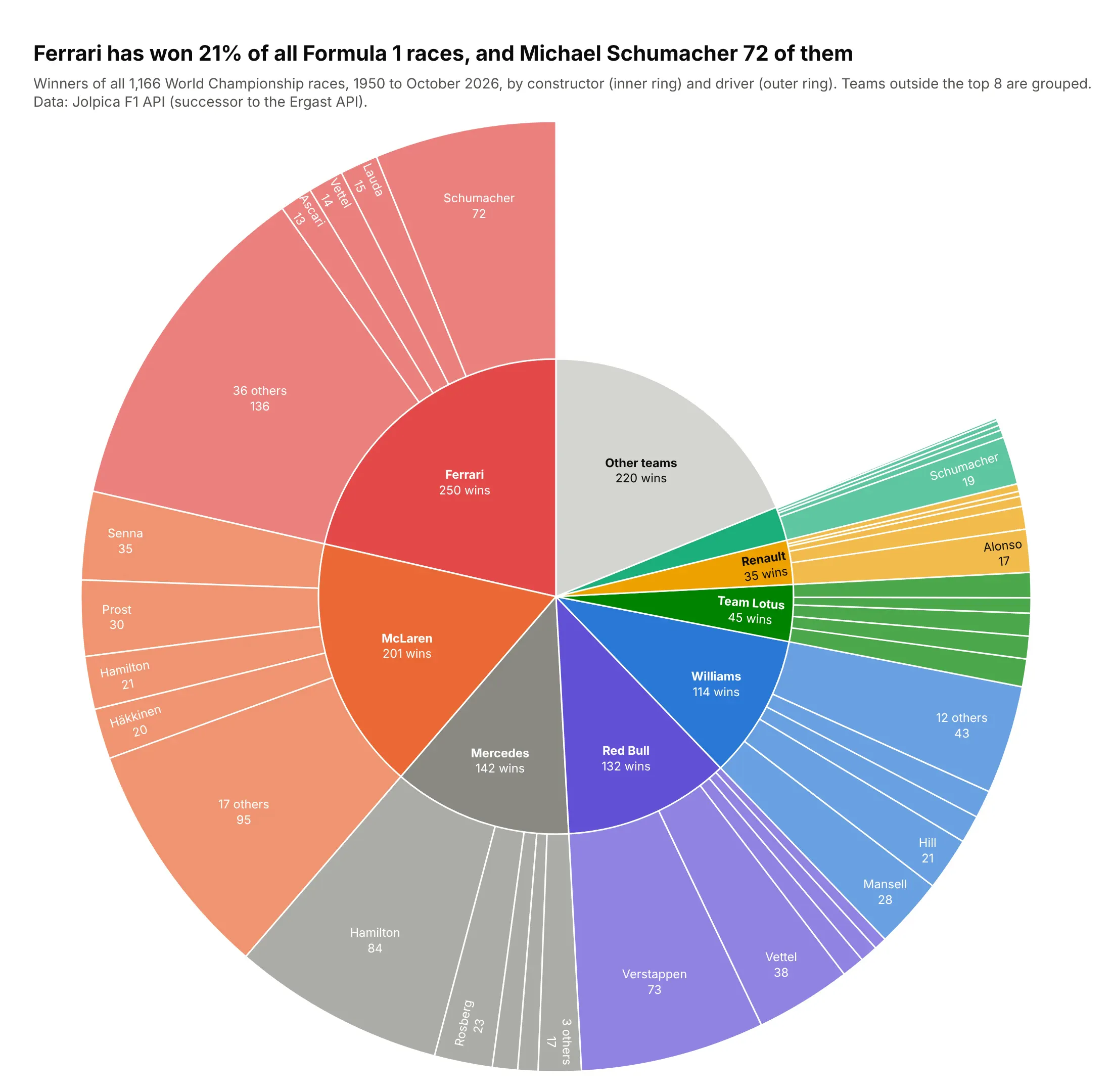
Ferrari has won 250 of 1,166 World Championship races (21%), and Michael Schumacher won 72 of them. Mercedes' 142 wins lean on Lewis Hamilton (84), and Red Bull's 132 on Max Verstappen (73). Data: Jolpica F1 API, 1950 to October 2026.

Tip: build ids from the path (team/driver), because drivers who won for two teams appear twice.