Chris Parmer

November 12, 2026

Load Duration Curves - A Complete Guide

TL;DR

A load duration curve takes every hour of a year of electricity demand, 8,760 of them, and sorts them from highest to lowest, so the x axis counts the hours the load was at least that high and the y axis shows the load in megawatts (MW) or gigawatts (GW, 1,000 MW). It shows how much capacity a grid needs for how many hours.
Load duration curves are also known as load-duration curves, LDCs and duration curves, and the same chart is called a flow duration curve in hydrology, a price duration curve for power prices and a net load duration curve when wind and solar are subtracted first. They are similar to empirical cumulative distribution function (ECDF) plots turned around, and to histograms of the same values.
Planners read it in bands: base load that runs all 8,760 hours, intermediate load and peak load that runs only a few hundred. In 2025 the Electric Reliability Council of Texas (ERCOT) needed 38.4 GW in every hour, but its top 11.7 GW in only 876 hours, at a capacity factor of 3.6%.
You can make a load duration curve with Plotly in Python by sorting the values with np.sort(load)[::-1] and drawing a go.Scatter line, or in one call with px.ecdf(df, y="load", ecdfmode="reversed", ecdfnorm=None). Code and prompts are below.

What is a load duration curve?

Load duration curves look like this:

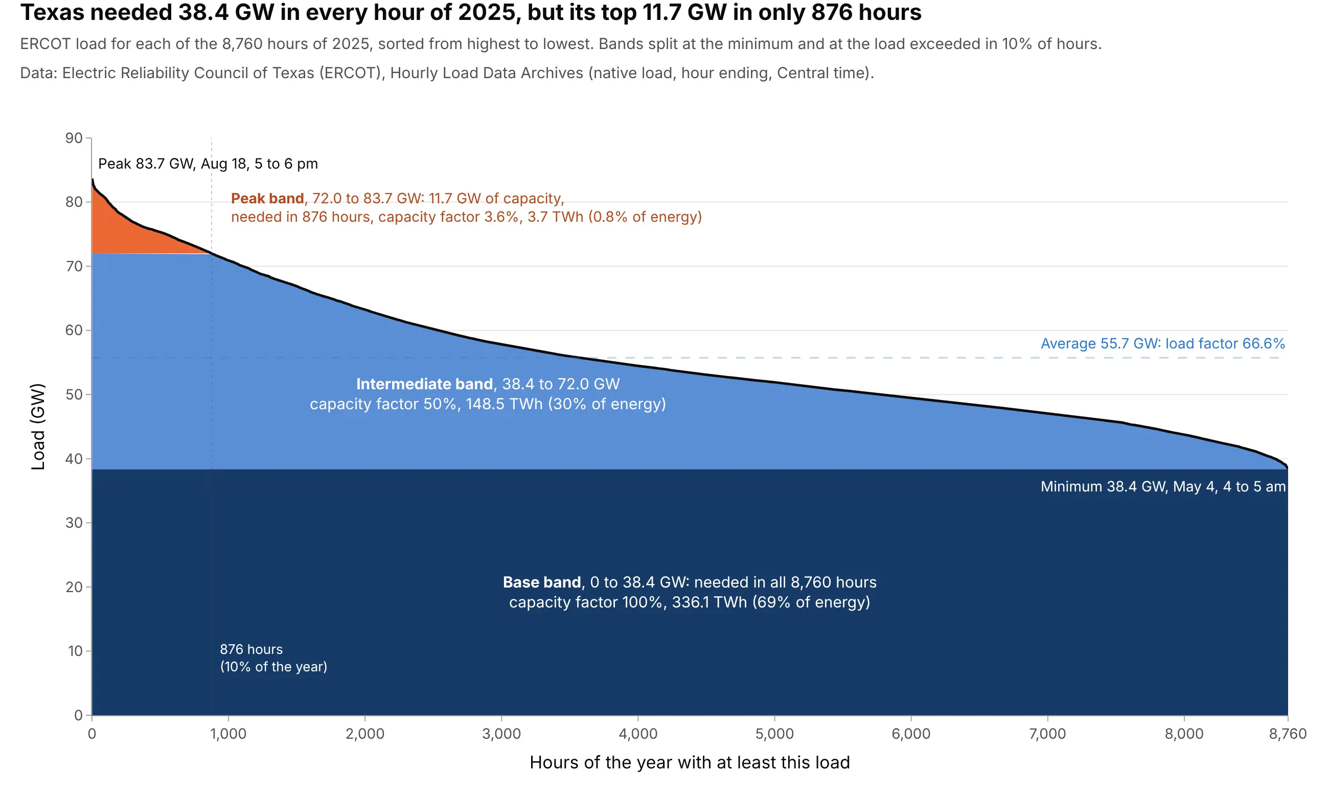
Load duration curve of ERCOT's 8,760 hourly loads in 2025, sorted from 83.7 GW at the left to 38.4 GW at the right, with the area underneath split into a dark blue base band up to 38.4 GW (all 8,760 hours, 336.1 TWh, 69% of energy), a lighter intermediate band from 38.4 to 72.0 GW (capacity factor 50%, 148.5 TWh) and an orange peak band from 72.0 to 83.7 GW needed in 876 hours (capacity factor 3.6%, 3.7 TWh, 0.8% of energy); a dashed line marks the average of 55.7 GW, a load factor of 66.6%

Data: Electric Reliability Council of Texas (ERCOT), Hourly Load Data Archives, native load for 2025.

How do you read a load duration curve? In the example above, notice these things:

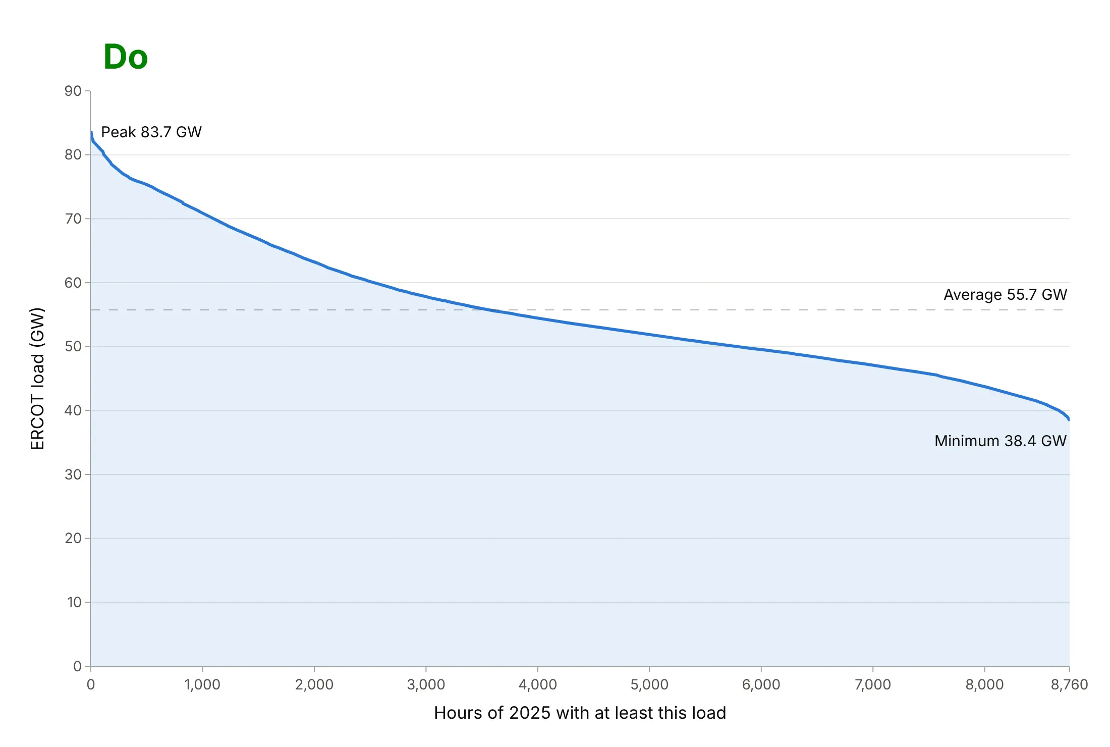
Every hour of 2025 is on the chart once, sorted from the highest load at the left to the lowest at the right. A point at 1,000 hours and 71 GW means the load was 71 GW or more in 1,000 hours of the year. The left end is the peak, 83.7 GW from 5 to 6 pm on August 18; the right end is the minimum, 38.4 GW from 4 to 5 am on May 4.
The y axis starts at zero, so the area under the curve is energy: 488.2 terawatt-hours (TWh, a million MWh) for the year. The dark base band, the 38.4 GW needed in every hour, holds 336.1 TWh of it, 69%.
The steep orange tip is the peak band. Capacity above 72.0 GW was needed in only 876 hours, 10% of the year, and delivered 3.7 TWh, 0.8% of the energy. A power plant sized for that slice would run at a capacity factor of 3.6%, its average output divided by its size.
The dashed line is the average load, 55.7 GW. Divided by the peak it gives the load factor, 66.6%: the flatter the curve, the closer the average is to the peak and the better a grid uses the capacity it has built.

It's often used for charts like these:

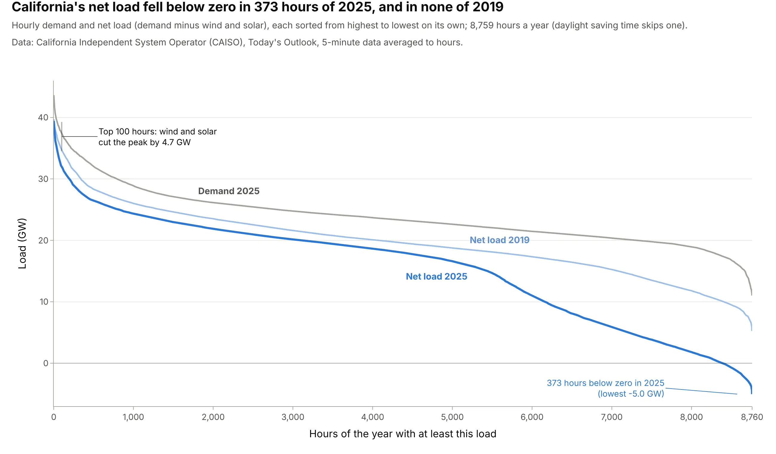
Load duration curves for California in two years: gray demand for 2025 from 43.6 GW down to about 11 GW, light blue net load (demand minus wind and solar) for 2019 that never falls below 5.3 GW, and blue net load for 2025 that falls below zero for its last 373 hours, to -5.0 GW; at the left, a bar shows that wind and solar cut the top 100 hours by 4.7 GW

Net load duration curves for renewable planning. Subtracting wind and solar before sorting shows what the rest of California's fleet has to cover: net load was below zero in 373 hours of 2025 and in none of 2019, while the top 100 hours fell by only 4.7 GW, a gap that planning models such as NREL's use as the capacity value of wind and solar (Cole et al. 2017). Data: California Independent System Operator (CAISO), Today's Outlook.

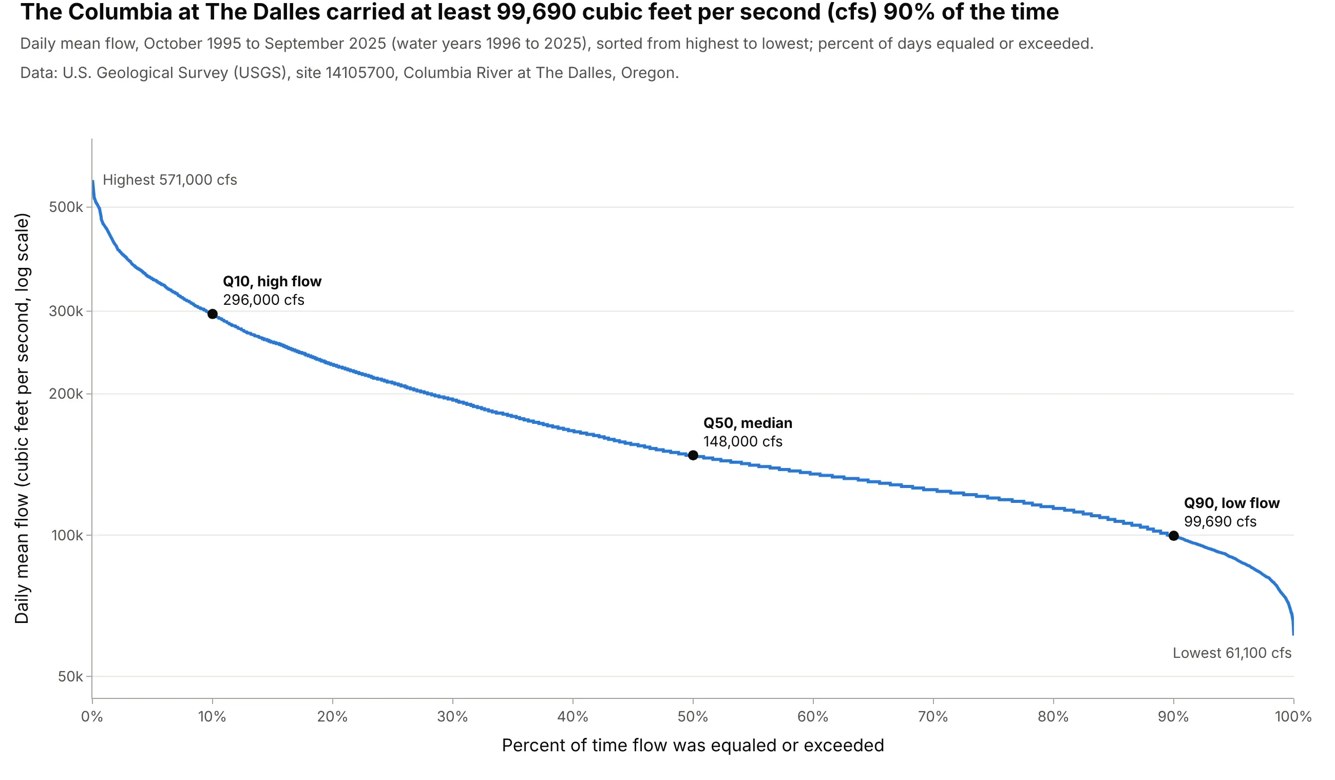
Flow duration curve of the Columbia River at The Dalles, Oregon: 10,958 daily mean flows from October 1995 to September 2025 on a log scale against the percent of time each was equaled or exceeded, falling from 571,000 cubic feet per second (cfs) to 61,100 cfs, with Q10 at 296,000 cfs, Q50 at 148,000 cfs and Q90 at 99,690 cfs marked

Flow duration curves in hydrology and hydropower, the classic use outside power systems. The Columbia at The Dalles carried at least 99,690 cubic feet per second (cfs) 90% of the time over 30 years, the flow hydrologists call Q90 and use for minimum flows and for sizing turbines. Data: U.S. Geological Survey (USGS), site 14105700.

A short history

Duration curves started with water. Hydrologists credit Clemens Herschel with the first flow duration curve around 1880 (Vogel and Fennessey 1994, citing Foster's 1934 paper "Duration curves"), and by 1959 the U.S. Geological Survey's manual said they had "been in general use since about 1915" (Searcy 1959). Hydropower engineers used them to decide how much water a plant could count on, and electric utilities sorted their hourly load the same way to decide how much of each kind of plant to build. The U.S. Energy Information Administration (EIA) still builds load duration curves from base, middle and peak periods in the models behind its long-term projections (EIA Handbook, section B3). Searcy's manual opens with the duration curve of Bouie Creek (he spells it Bowie) in Mississippi, and says the creek's daily flow "was at least 144 cubic feet per second during 90 percent of the time". Here it is redrawn from the same USGS record:

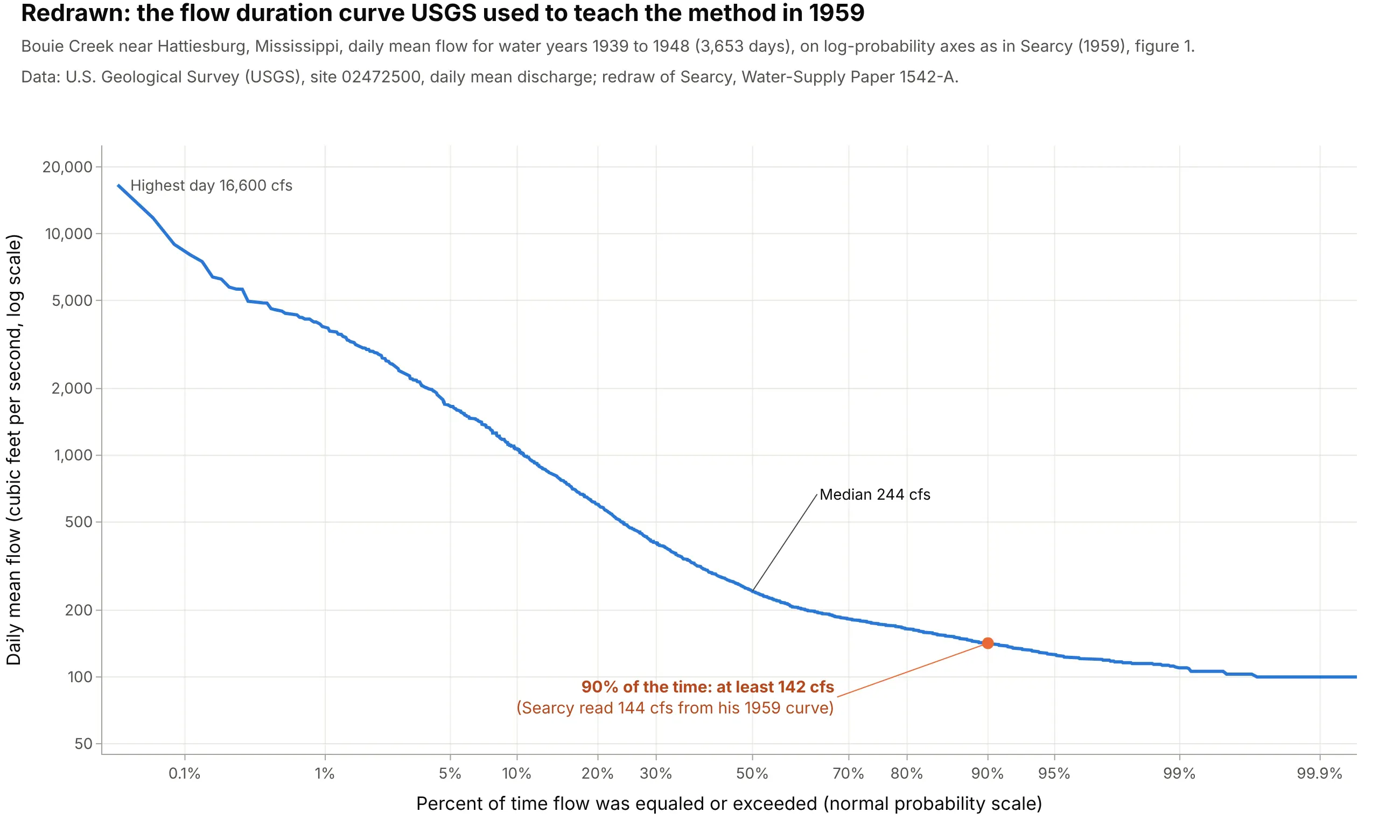
Redraw of Searcy's 1959 figure 1: the flow duration curve of Bouie Creek near Hattiesburg, Mississippi, for water years 1939 to 1948, 3,653 daily flows on log-probability axes, from 16,600 cfs on the highest day to 100 cfs, with the median of 244 cfs and the 90% point at 142 cfs marked, next to Searcy's reading of 144 cfs

Data: USGS, site 02472500, daily mean discharge; redraw of Searcy (1959), figure 1. Searcy built his curve from class intervals, the record read directly gives 142 cfs at 90%, and 89% of the days were at or above his 144 cfs. The x axis is a normal probability scale, which spreads out the rare high and low flows at both ends, as on the paper he used.

How a load duration curve works

A load duration curve throws away the time of day and the date and keeps only how often each level happened. These are the ideas behind it, in the order a grid planner uses them.

Sorting turns a year into a duration curve

Take the 8,760 hourly loads of a year in time order, sort them from highest to lowest, and number them from 1 to 8,760. That number is the duration: how many hours the load was at least this high. The peak hour becomes hour 1, the quietest hour becomes hour 8,760, and a typical hour lands in the middle:

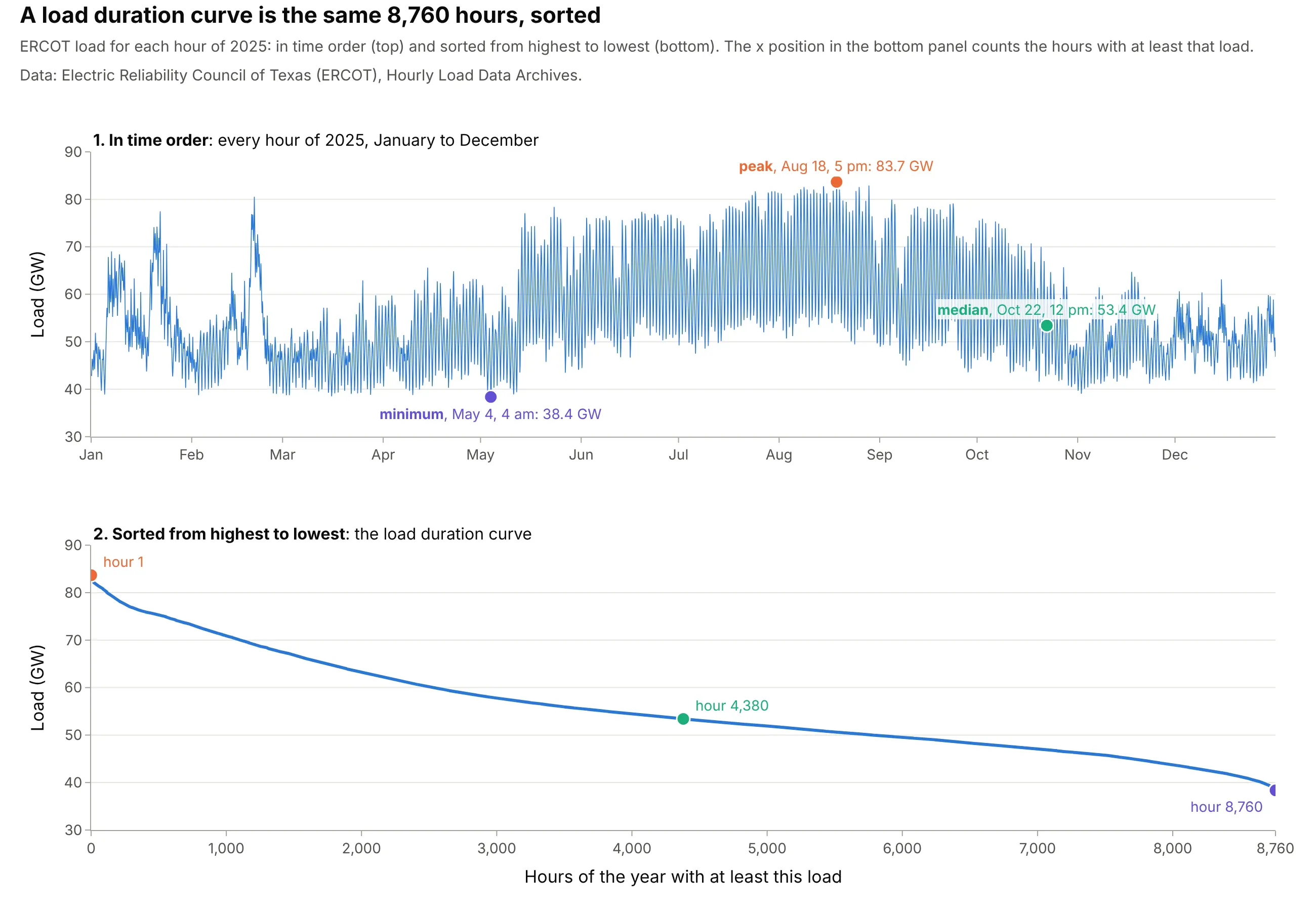
Two panels of ERCOT's 2025 hourly load: on top the 8,760 hours in time order from January to December, with the peak on August 18 at 83.7 GW, a median hour on October 22 at 53.4 GW and the minimum on May 4 at 38.4 GW marked in orange, green and purple; below, the same values sorted from highest to lowest, where the three marked hours land at hour 1, hour 4,380 and hour 8,760

Data: ERCOT, Hourly Load Data Archives, 2025.

Because sorting forgets the order, the curve doesn't care about time stamps, daylight saving time or hour-ending conventions, so the messy clocks of grid data can't shift it. It also means two hours at the same position on two curves are usually different hours, which matters when you compare demand and net load (the FAQ explains why).

It's an ECDF turned around

Statisticians would call a load duration curve a complementary cumulative distribution function (Wikipedia; Vogel and Fennessey 1994 say the same of flow duration curves). An ECDF plot shows the share of values at or below each level; a duration curve shows the share at or above it, with the axes swapped so the load is on the y axis:

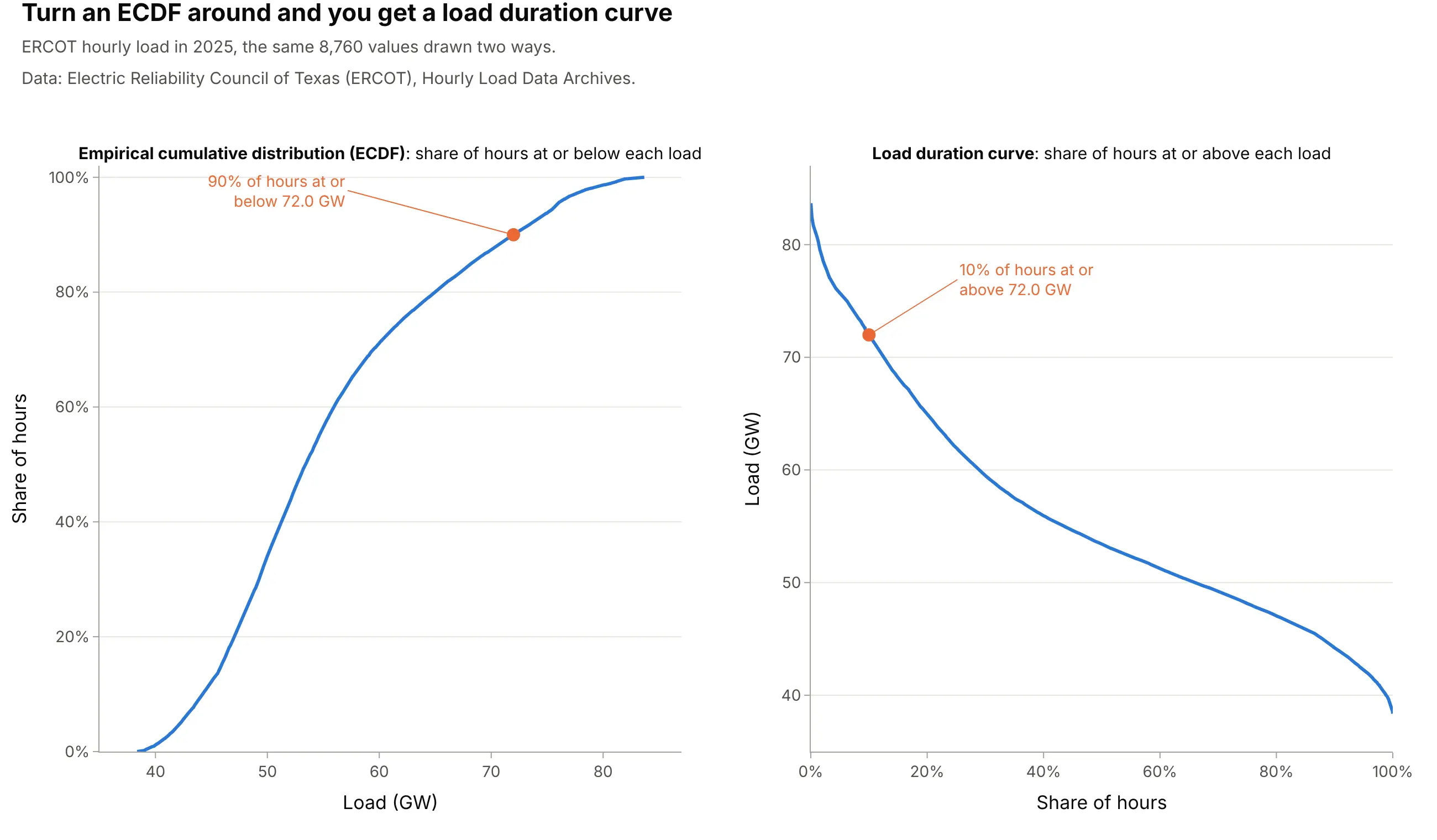
Two panels of ERCOT's 2025 hourly load: on the left an empirical cumulative distribution (ECDF) rising from 0% at 38 GW to 100% at 84 GW, with 90% of hours at or below 72.0 GW marked; on the right the load duration curve falling from 84 GW to 38 GW against the share of hours, with 10% of hours at or above 72.0 GW marked at the same point

Data: ERCOT, Hourly Load Data Archives, 2025.

That's why Plotly's px.ecdf can draw one directly (see the code below), and why hydrologists label points by the percent of time a flow was equaled or exceeded: Q90 is the flow exceeded 90% of the time, a low flow, and Q10 a high one.

Base, intermediate and peak load

Power plants differ in what they cost to build and to run. A plant that is expensive to build but cheap to run pays off only if it runs most of the year, while one that is cheap to build but expensive to run makes sense for the few hours when the load is highest; EIA notes that suppliers "often use different generating technologies for peak load generation than they use for the continuous base load generation". A load duration curve shows how much capacity falls in each group, and EIA's models split the year into base, middle and peak periods for the same reason. The base load is the level the load never drops below, needed all year; the peak load is the slice at the top needed only in the highest hours; intermediate load is in between. Where to draw the line between intermediate and peak depends on the plants' costs, so this guide draws it at the load exceeded in 10% of the hours and says so on the chart.

Load factor and capacity factor

Two ratios come straight off the curve. The load factor is the average load divided by the peak: 55.7 / 83.7 GW = 66.6% for ERCOT in 2025. The capacity factor of a plant is its energy over a year divided by what it would produce running at full output all year. For a slice of the curve, it's the area of the slice divided by its height times 8,760 hours, which is why the thin orange tip of the main example has a capacity factor of only 3.6% while the base band's is 100%.

Alternatives to a load duration curve

Here's the same year of Texas load drawn six ways. Some are better for the question, some worse, some just different:

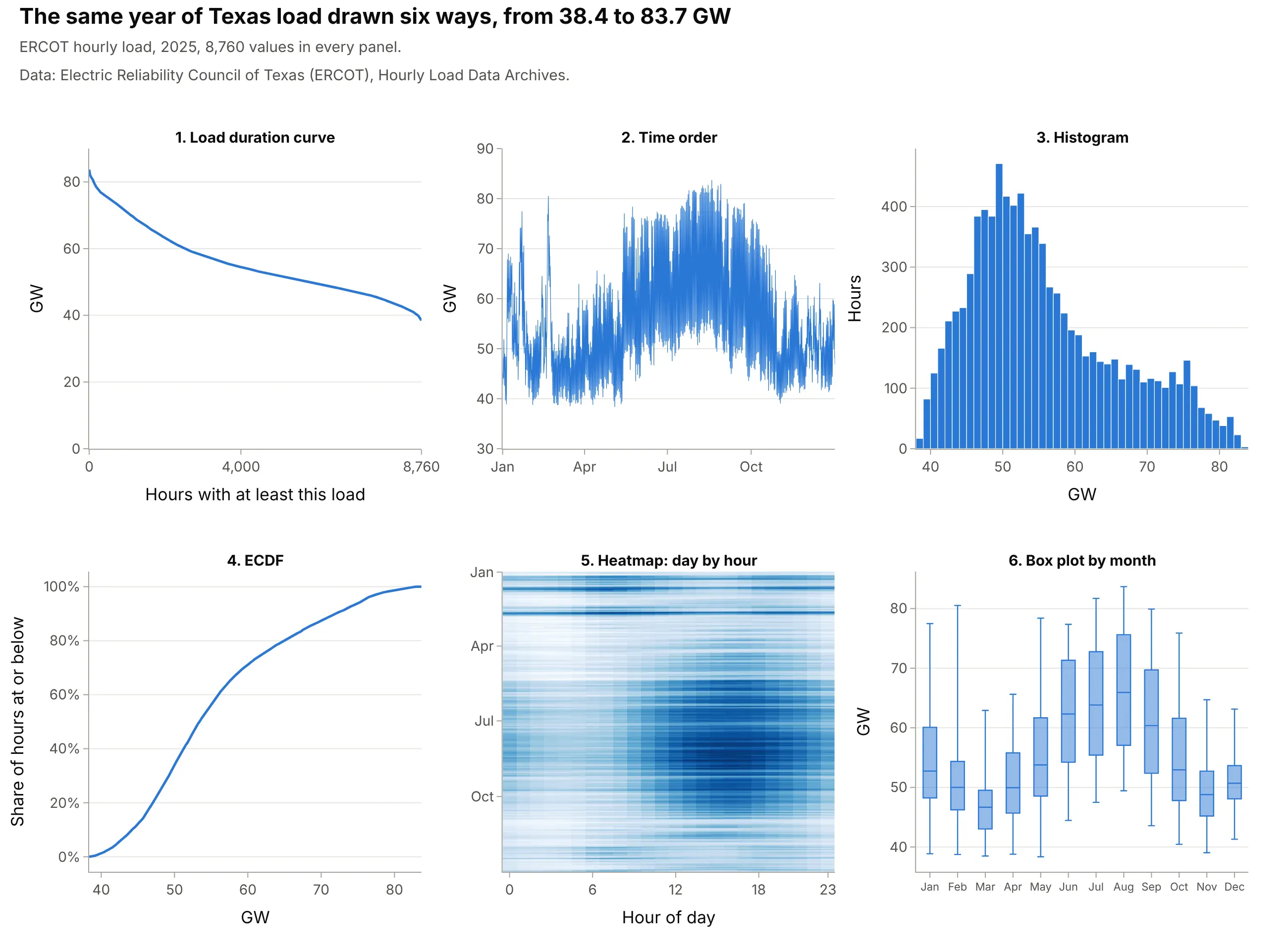
ERCOT 2025 hourly load in six panels: 1, the load duration curve; 2, the 8,760 hours in time order, a dense line peaking in August; 3, a histogram with most hours between 45 and 55 GW and a long tail to 83 GW; 4, an ECDF rising from 38 to 84 GW; 5, a heatmap of days by hour of day, darkest on summer afternoons; 6, box plots by month, highest in August

Line chart in time order (different). It shows when the peaks happened (August afternoons, 80.5 GW on a cold February morning) but you can't read how many hours were above 72 GW from it. Use a line chart for when, and the duration curve for how long.
Histogram (worse for sizing capacity). It shows the most common loads, 45 to 55 GW, but the hours above a level are the area of the tail, which is hard to read off bars.
ECDF (works too). The same information with the axes swapped; statisticians read it more easily, power and water engineers expect the duration curve.
Heatmap of day by hour (better for when). It keeps the time of day and the season that the duration curve throws away, so it shows that the peak hours are summer afternoons. The duck curve guide uses the same view for net load.
Box plot by month (different). It compares seasons, but the extremes become whiskers and the hours above a level disappear.

How to make a load duration curve

With AI

ChatGPT, Claude Code, GitHub Copilot, Cursor and other AI tools are excellent at writing Plotly code. Name Plotly in the prompt, and say how to sort, which units to use and where the y axis starts:

Make a plotly load duration curve from ercot_2025.csv (columns: hour_ending, ERCOT = hourly load in MW).

- Sort the 8,760 loads from highest to lowest and plot them against hours 1 to 8,760 as a line, in GW.
- x axis: "Hours of the year with at least this load", 0 to 8,760; y axis: "Load (GW)" starting at zero.
- Shade three bands: base (below the minimum), intermediate, and peak (above the load exceeded in 876 hours).
- Label the peak, the minimum and the average, and print the load factor and each band's capacity factor.

With Plotly Studio

Plotly Studio is a desktop app where you point an AI at a dataset and it builds charts and a Dash app around your questions. Ask for a load duration curve the same way:

Show a load duration curve of hourly load for the selected year, sorted from highest to lowest in GW, with a dropdown for the weather zone, a toggle to divide by the zone's peak, and the load factor in the title.

Make a load duration curve in Python or JavaScript

This is the code AI tools write under the hood. Plotly has no special duration curve trace, and it doesn't need one: sort the values from highest to lowest and draw them as a line against their rank.

import numpy as np
import pandas as pd
import plotly.graph_objects as go

df = pd.read_csv("ercot_2025.csv")                     # one row per hour: hour_ending, ERCOT load in MW
load = np.sort(df["ERCOT"].to_numpy())[::-1] / 1000    # GW, highest first
hours = np.arange(1, len(load) + 1)                    # hour 1 is the peak

fig = go.Figure(go.Scatter(x=hours, y=load, mode="lines", fill="tozeroy"))
fig.update_xaxes(title="Hours of the year with at least this load", range=[0, 8760])
fig.update_yaxes(title="Load (GW)", rangemode="tozero")
fig.show()

You can make the same curve in one line of code with Plotly Express, which counts the hours at or above each value for you: px.ecdf(df, y="ERCOT", ecdfmode="reversed", ecdfnorm=None). For a flow duration curve, use percent of time on x (100 * rank / (n + 1)) and fig.update_yaxes(type="log").

In JavaScript, plotly.js draws it from any array once it's sorted:

<div id="chart"></div>
<script src="https://cdn.plot.ly/plotly-4.1.1.min.js"></script>
<script>
  // ERCOT load (MW) for the 24 hours of August 18, 2025, the day of the 2025 peak; use all 8,760 hours for a year
  const load = [61762, 58836, 57000, 56038, 55715, 56628, 58273, 58694, 61491, 65702, 70581, 75552,
                79962, 82402, 82792, 83098, 83674, 83679, 82858, 80518, 78502, 74366, 70056, 66269];
  const sorted = [...load].sort((a, b) => b - a);   // highest first
  const hours = sorted.map((_, i) => i + 1);          // hour 1 is the peak

  Plotly.newPlot("chart", [{x: hours, y: sorted.map(v => v / 1000), mode: "lines", fill: "tozeroy"}], {
    width: 900, height: 500,
    xaxis: {title: {text: "Hours with at least this load"}},
    yaxis: {title: {text: "Load (GW)"}, rangemode: "tozero"}
  });
</script>

Share it

Every Plotly chart has a Share chart button (the cloud icon in its toolbar) that uploads it to Plotly Cloud and gives you a link. Only you can see it until you change its visibility.

For a live app, put the chart in a Dash app and publish it with the Plotly Cloud command-line interface (CLI). Coding agents can run these commands for you:

pip install "dash[cloud]"
plotly user login
plotly app publish

If your data has to stay in your own cloud or data center, publish to Dash Enterprise instead.

Dos and don'ts

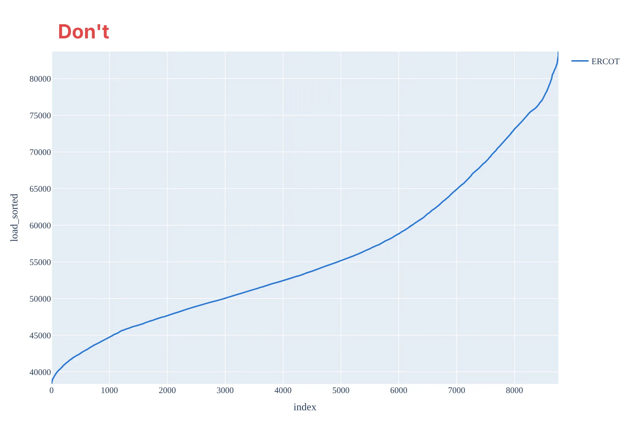
Most mistakes on a load duration curve come from treating it like any other sorted line: the wrong direction, an axis that starts at the minimum and raw column names.

Don't sort from lowest to highest, label the x axis with row numbers, start the y axis at the minimum load, which makes the peak look more than twice the base and stops the area from meaning energy, or keep raw megawatts without separators, a one-line legend, a gray background and a serif font:

ERCOT 2025 load sorted from lowest to highest, rising from 38,363 at the left to 83,679 at the right, on a gray background with a serif font, an x axis titled index from 0 to 8000, a y axis titled load_sorted that starts at 38,363 with raw tick labels like 80000, and a legend with one entry, ERCOT

Do sort from highest to lowest, count hours from 0 to 8,760, start the y axis at zero, use GW and label the peak, the minimum and the average:

The same data sorted from highest to lowest, 83.7 GW at the left down to 38.4 GW at the right, with the area under the curve lightly shaded, an x axis of hours of 2025 from 0 to 8,760, a y axis of ERCOT load in GW from 0 to 90, and labels for the peak of 83.7 GW, the minimum of 38.4 GW and a dashed average of 55.7 GW

Checklist

Sort from highest to lowest and say what one step on the x axis is (an hour, a day, a 5-minute interval).
Start the y axis at zero when the area matters, so bands and energy read honestly.
Say how many values went in and what was missing (8,736 hours, not 8,760, when a day is missing).
Divide by each grid's peak, or use the percent of time, when you compare grids or years of different size.
Use a log y axis and percent of time for streamflow, the hydrology convention.

Don't

Expect the hours on two curves to line up: the 100th hour of demand and the 100th hour of net load are usually different hours.
Call the bands facts; where peak ends and intermediate begins is a choice, so say how you drew it.
Average many years into one curve without saying so; one curve per year shows the dry or hot years.
Read the time of day off a duration curve; it has none, so pair it with a heatmap when the timing matters.

Options to customize

A load duration curve in Plotly is a sorted line chart, so these are the options that matter most. The full lists are in the scatter trace reference, the px.ecdf reference and the axes documentation.

np.sort(values)[::-1] with np.arange(1, n + 1): the curve itself, highest value first and the hour count on x.
px.ecdf(df, y="load", ecdfmode="reversed", ecdfnorm=None): the same curve in one call, with the count of hours at or above each value on x; ecdfnorm="percent" gives the percent of time instead.
fill="tozeroy": shades the area under the curve, which is the energy.
fill="tonexty" on a second trace: shades bands between two levels, such as base, intermediate and peak.
fig.update_yaxes(rangemode="tozero"): keeps zero on the axis so areas compare honestly.
fig.update_yaxes(type="log"): the hydrology convention for flow duration curves, which span several orders of magnitude.
tickvals and ticktext: hour ticks such as 0, 2,000 ... 8,760, or normal-probability ticks (0.1%, 1%, 10%, 50% ...) placed with scipy.stats.norm.ppf.
fig.add_hline(y=...) and fig.add_vline(x=...): the average load, a band boundary or the 876-hour line.
facet_col="grid" in Plotly Express: small multiples of several grids or zones on shared axes.
go.Scattergl: WebGL for millions of points, though a sorted curve rarely needs them (see the FAQ).

More load duration curve examples

Eight more duration curves built from real public data, each with its source, the technique that makes it work, and a prompt to rebuild it.

1. A price duration curve: below zero in 976 hours

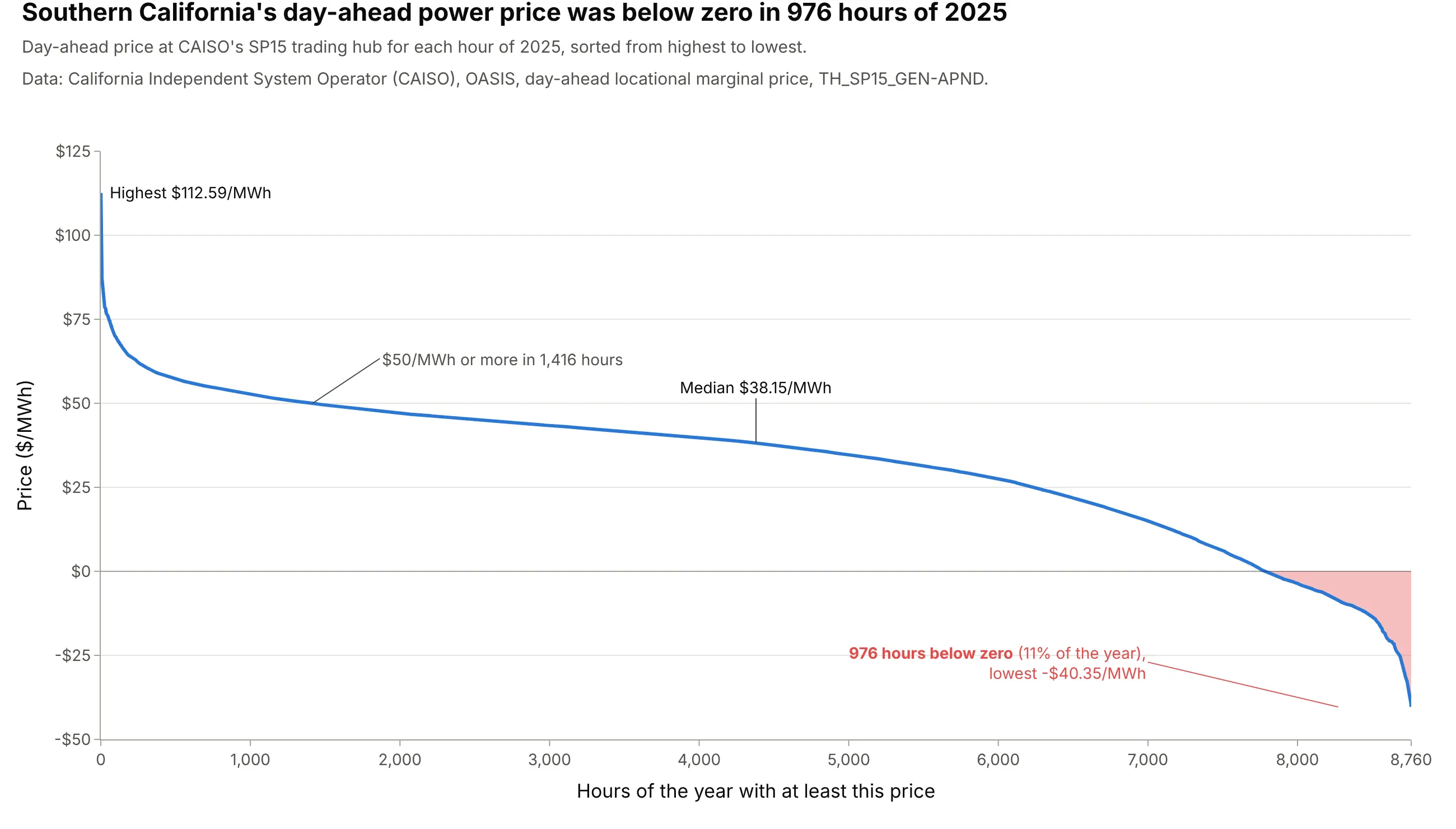
Price duration curve of the day-ahead price at CAISO's SP15 trading hub for each hour of 2025, sorted from $112.59/MWh at the left to -$40.35/MWh at the right, with a median of $38.15/MWh, 1,416 hours at $50/MWh or more, and the last 976 hours, 11% of the year, below zero and shaded red

A price duration curve sorts hourly prices the way a load duration curve sorts load. At CAISO's SP15 trading hub for Southern California, the day-ahead price was below zero in 976 hours of 2025, 11% of the year, and $50 per megawatt-hour (MWh) or more in 1,416. A battery or power plant developer can count from it how many hours a year are worth selling in. Data: CAISO, Open Access Same-time Information System (OASIS), day-ahead locational marginal price (LMP), TH_SP15_GEN-APND.

Tip: fill the area below zero in a warning color so the negative hours read as a count, not a dip.

Get the data from CAISO's OASIS API (oasis.caiso.com/oasisapi, query PRC_LMP, market DAM, node TH_SP15_GEN-APND,
hourly day-ahead price in $/MWh, at most 31 days per request) for 2025 (columns: date, hour_ending, price).

Build a plotly price duration curve: prices sorted from highest to lowest against hours 1 to 8,760, a zero line,
the part below zero filled red and labeled with its number of hours, and the median labeled.

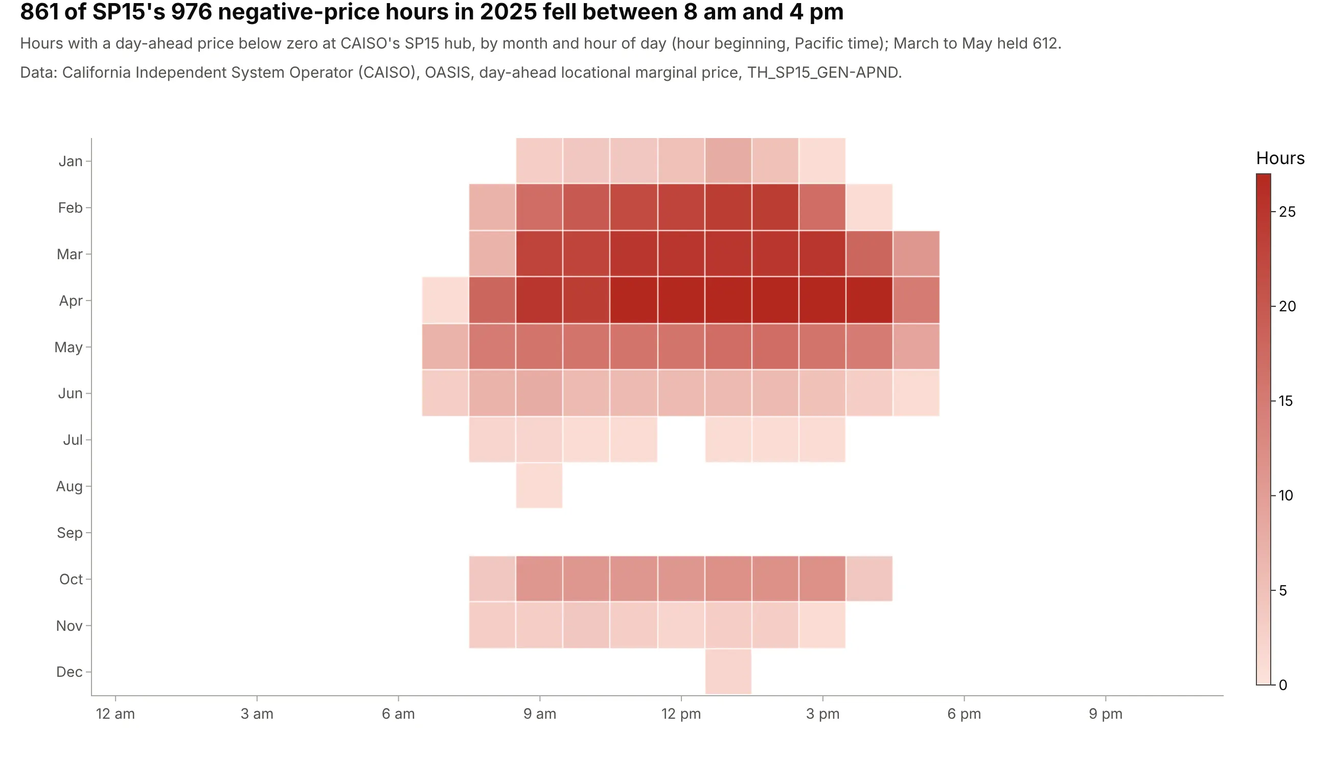
Another way to see it: a heatmap of the negative hours by month and hour of day puts the time back. 861 of the 976 fell between 8 am and 4 pm, and 612 between March and May, when solar output is high and demand is mild:

Heatmap of the number of negative-price hours at SP15 in 2025 by month (rows) and hour of day (columns): all between about 7 am and 6 pm, darkest from February to May around noon, with up to 27 hours per cell in April, lighter in June and October, and almost none from July to September

2. Texas over two decades: the bottom of the curve rose fastest

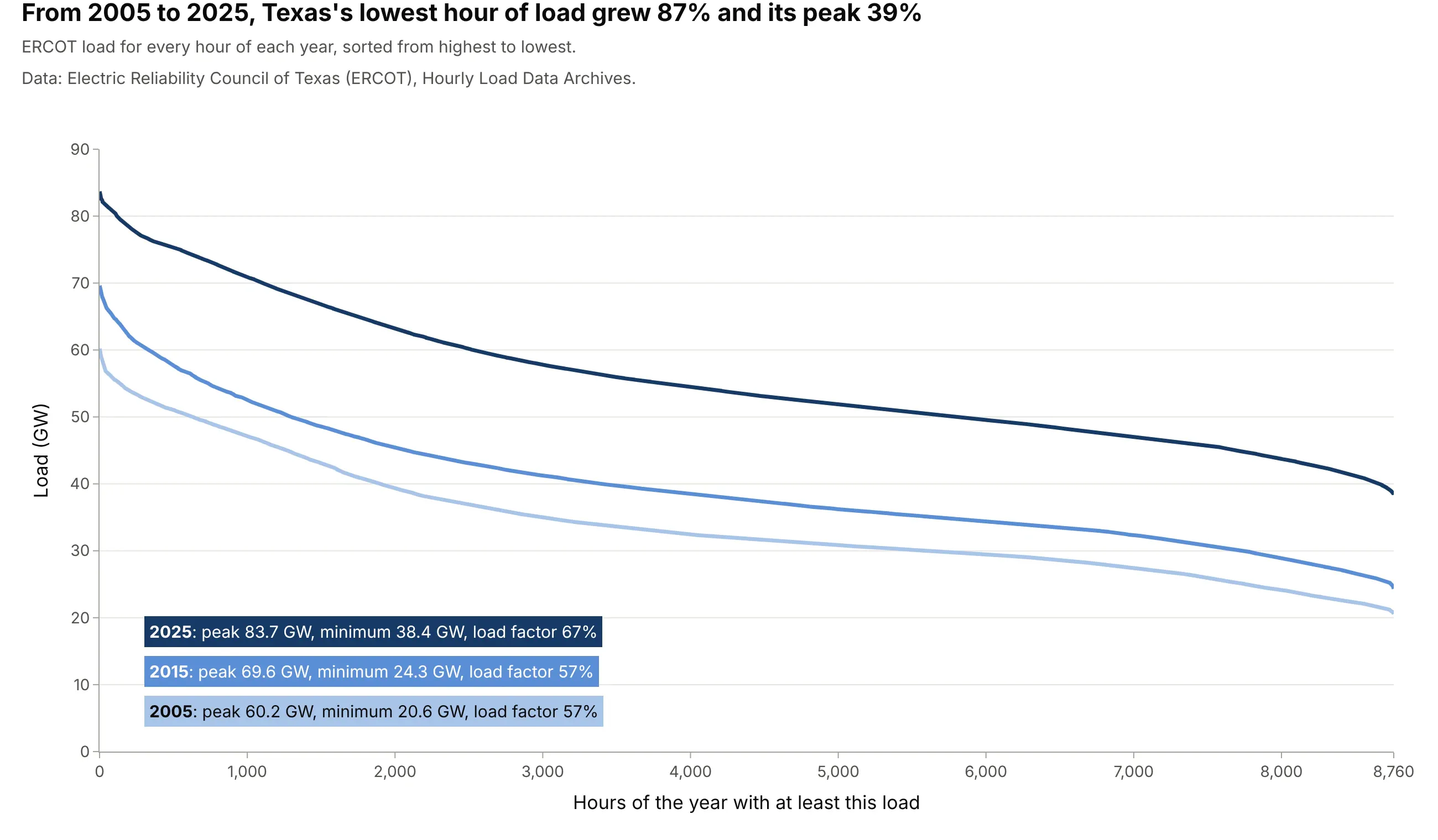
ERCOT load duration curves for 2005, 2015 and 2025 in light to dark blue: 2005 from 60.2 GW down to 20.6 GW with a load factor of 57%, 2015 from 69.6 to 24.3 GW (57%), and 2025 from 83.7 to 38.4 GW (67%), the 2025 curve higher and flatter than the others

From 2005 to 2025 ERCOT's lowest hour grew 87%, from 20.6 to 38.4 GW, while its peak grew 39%, from 60.2 to 83.7 GW. The curve flattened and the load factor rose from 57% to 67%, which means the growth came from load that runs around the clock. Data: ERCOT, Hourly Load Data Archives.

Tip: use one hue from light to dark so the years read in order, and put the key numbers in a colored key instead of a legend.

Get the data from ERCOT's Hourly Load Data Archives (ercot.com/gridinfo/load/load_hist, one workbook per year with
hourly load in MW by weather zone and an ERCOT total) for 2005, 2015 and 2025 (columns: year, hour_ending, ERCOT).

Build a plotly chart with one load duration curve per year in light to dark blues, y axis in GW from zero, and a
key that gives each year's peak, minimum and load factor.

3. Far West Texas runs almost flat out

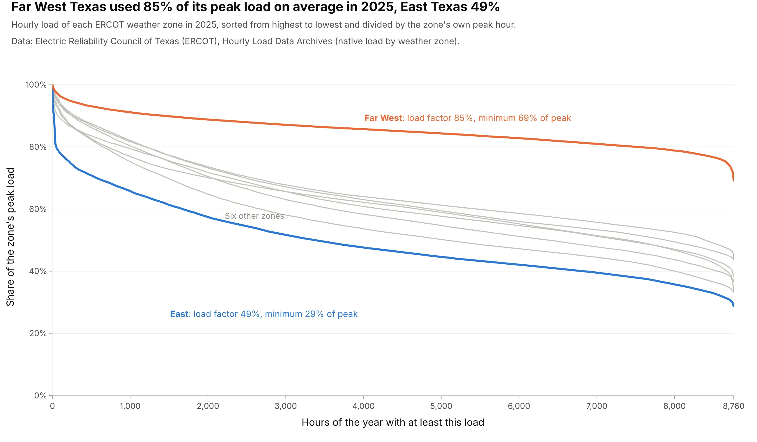
Load duration curves of ERCOT's eight weather zones in 2025, each divided by its own peak: Far West in orange stays between 100% and 69% of its peak with a load factor of 85%, East in blue drops quickly to about 70% and ends at 29% with a load factor of 49%, and six other zones in light gray in between

Dividing each zone by its own peak puts zones of very different size on one axis. In 2025 Far West Texas averaged 85% of its peak load and never fell below 69% of it, while East Texas averaged 49%. ERCOT puts the Far West's peak growth at about 11% a year over the last decade, "driven by the significant growth in oil and natural gas industry demand" in the Permian Basin (ERCOT 2024). Data: ERCOT, Hourly Load Data Archives, native load by weather zone.

Tip: highlight the two zones you're comparing and leave the rest in light gray as context.

Get the data from ERCOT's Hourly Load Data Archives (ercot.com/gridinfo/load/load_hist, Native_Load_2025: hourly
load in MW for eight weather zones) (columns: hour_ending, Coast, East, Far West, North, North Central, South,
South Central, West).

Build a plotly chart of each zone's load duration curve divided by its own peak, Far West in orange and East in
blue with their load factors labeled, the other zones light gray.

4. The top of the curve: 179 hours for the last 5 GW

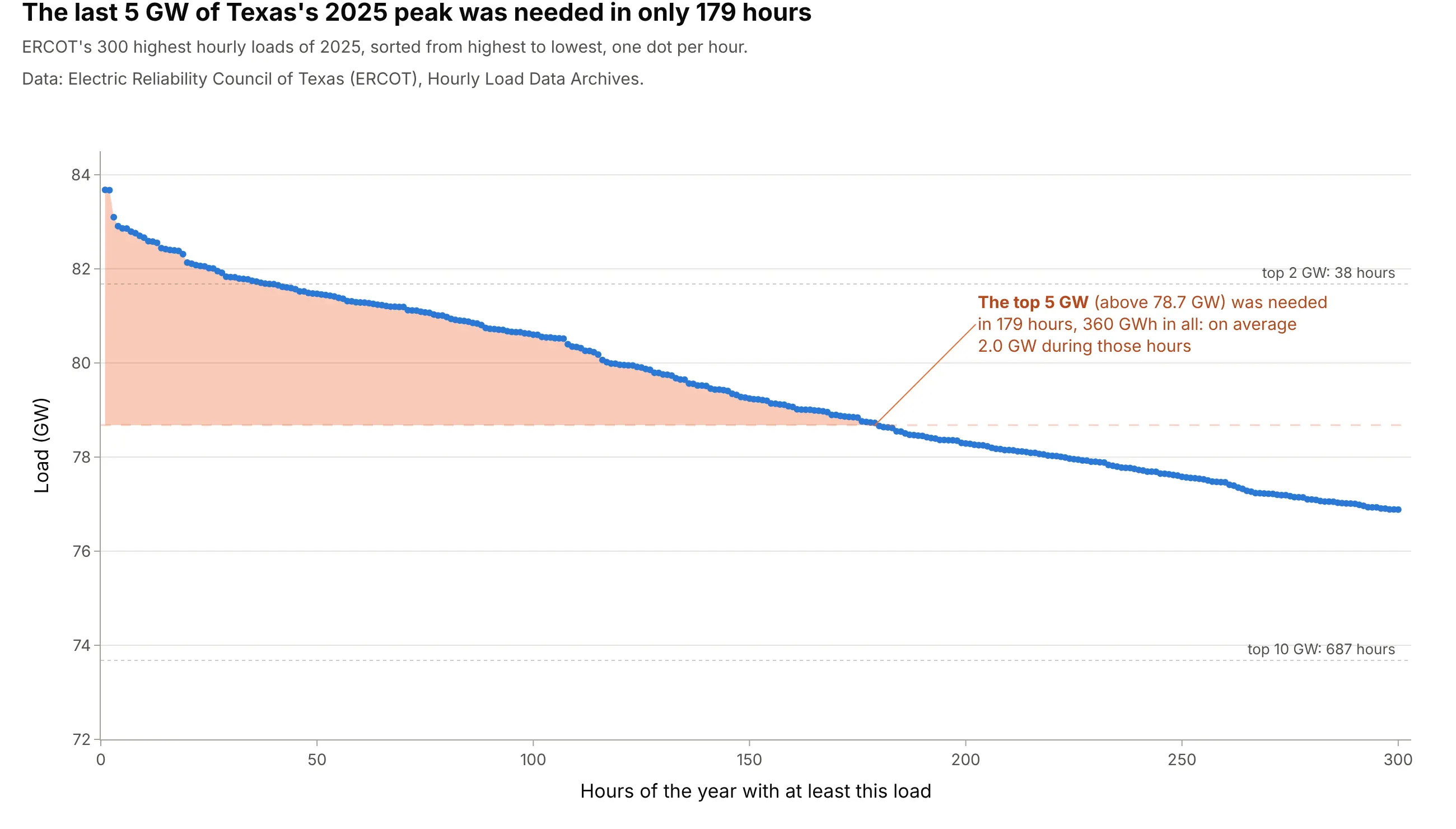
ERCOT's 300 highest hourly loads of 2025 as dots from 83.7 GW down to 76.9 GW, with the area above 78.7 GW shaded orange: the top 5 GW was needed in 179 hours and 360 GWh in all; dotted lines mark the top 2 GW at 38 hours and the top 10 GW at 687 hours

Zooming into the steep left end shows how little energy the last few gigawatts carry. ERCOT's top 5 GW in 2025 was needed in 179 hours and delivered 360 gigawatt-hours (GWh), an average of 2.0 GW during those hours; the top 2 GW was needed in 38 hours. That slice is what demand response, paying large customers to use less, and peaking plants are sized for. Data: ERCOT, Hourly Load Data Archives.

Tip: draw one dot per hour when you zoom in, so readers can count the hours above a line.

Get the data from ERCOT's Hourly Load Data Archives (ercot.com/gridinfo/load/load_hist, Native_Load_2025: hourly
ERCOT load in MW) (columns: hour_ending, ERCOT).

Build a plotly chart of the 300 highest hours sorted from highest to lowest as dots, in GW, with the area above
"peak minus 5 GW" shaded and labeled with its number of hours and its energy in GWh.

5. Generation duration curves: wind and solar in Texas

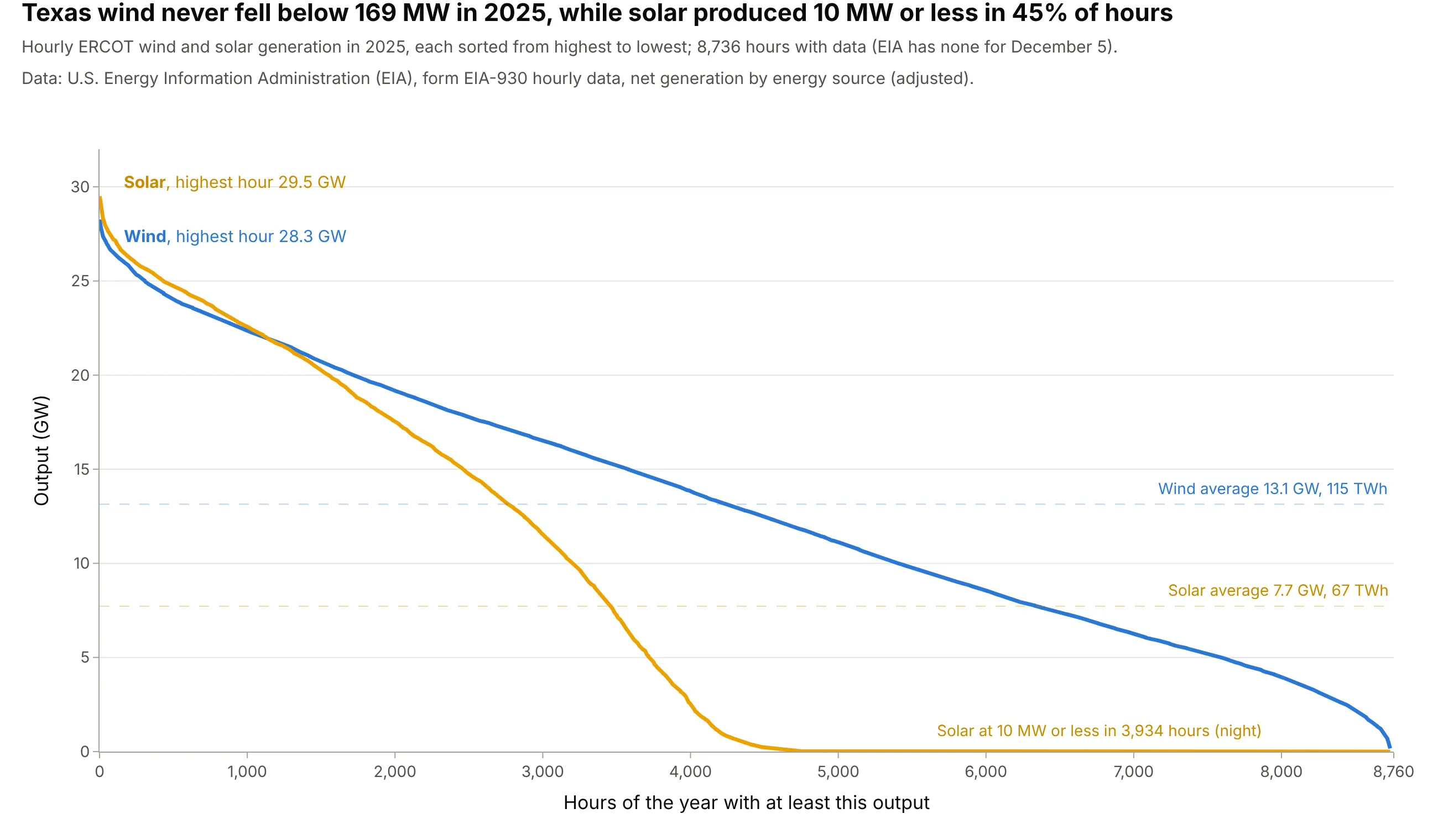
Duration curves of ERCOT's hourly wind and solar output in 2025: wind in blue falls from 28.3 GW to 169 MW with an average of 13.1 GW and 115 TWh, while solar in yellow starts higher at 29.5 GW, crosses below wind after about 1,200 hours and sits at zero for its last 3,934 hours, the night, with an average of 7.7 GW and 67 TWh

The same sort works for a power source's output. Texas solar reached a higher hour than wind in 2025, 29.5 GW against 28.3 GW, but produced 10 MW or less in 3,934 hours, the nights, so it delivered 67 TWh against wind's 115. Wind never fell below 169 MW. Data: EIA, Hourly Electric Grid Monitor (form EIA-930), ERCOT net generation by energy source; 8,736 hours, since EIA has no data for December 5.

Tip: draw each source's average as a dashed line in its color; the area under each curve is its year's energy.

Get the data from EIA's Hourly Electric Grid Monitor six-month files (eia.gov/electricity/gridmonitor/sixMonthFiles,
form EIA-930: hourly net generation in MW by energy source for every balancing authority) for ERCOT in 2025
(columns: local_start, solar, wind).

Build a plotly chart of a duration curve for wind and for solar, each sorted on its own, in GW, with each average
as a dashed line and the hours of near-zero solar labeled.

6. Six US grids on one scale

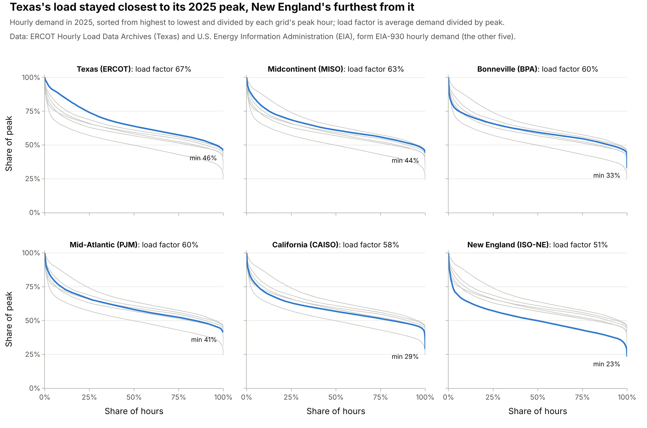
Six small panels of 2025 load duration curves divided by each grid's peak, each highlighting one grid over the others in gray: Texas (ERCOT) load factor 67% and minimum 46% of peak, Midcontinent (MISO) 63% and 44%, Bonneville (BPA) 60% and 33%, Mid-Atlantic (PJM) 60% and 41%, California (CAISO) 58% and 29%, and New England (ISO-NE) 51% and 23%

With both axes in percent, grids of 11 to 160 GW share one scale. ERCOT had the flattest curve in 2025, a load factor of 67%, and ISO New England (ISO-NE) the steepest, 51%, with its quietest hour at 23% of its peak. The other grids are the Midcontinent Independent System Operator (MISO), the Bonneville Power Administration (BPA), PJM, which runs much of the Mid-Atlantic and Midwest, and CAISO. Data: ERCOT Hourly Load Data Archives (Texas) and EIA-930 hourly demand (the other five).

Tip: in small multiples, draw every other grid in light gray behind the highlighted one, so each panel is a comparison.

Get the data from EIA's Hourly Electric Grid Monitor six-month files (eia.gov/electricity/gridmonitor/sixMonthFiles,
form EIA-930: hourly demand in MW for every balancing authority) for CISO, PJM, MISO, ISNE and BPAT in 2025
(columns: ba, utc_end, demand).

Build plotly small multiples, one panel per grid sorted by load factor, each a load duration curve with x as the
share of hours and y as the share of the grid's peak, the other grids in light gray, load factor in the panel title.

7. One flow duration curve per year: the Columbia in a dry year

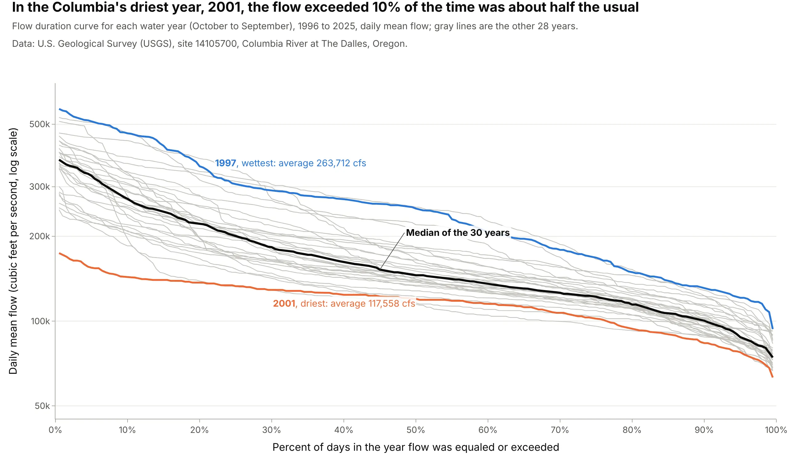
Thirty annual flow duration curves of the Columbia River at The Dalles, water years 1996 to 2025, in light gray on a log scale, with the median of the 30 in black, the wettest year 1997 in blue (average 263,712 cfs) and the driest year 2001 in orange (average 117,558 cfs), whose high flows stay below about 180,000 cfs

A curve over 30 years hides how a single year behaves, so hydrologists also draw one per year and take the median across them (Vogel and Fennessey 1994). In 2001, the Columbia's driest year in the record shown, the flow exceeded 10% of the time was 143,400 cfs, 53% of the median year's 271,800, while its low flow, Q90, was 83% of the median year's. Data: USGS, site 14105700, daily mean discharge.

Tip: interpolate each year's curve onto the same percent grid before you take the median across years.

Get the data from the USGS daily values service (waterservices.usgs.gov/nwis/dv, site 14105700, parameter 00060:
daily mean discharge in cubic feet per second) for October 1995 to September 2025 (columns: date, flow_cfs).

Build a plotly chart with one flow duration curve per water year (October to September) in light gray, on a log y
axis against the percent of days exceeded, the median of the yearly curves in black, and the driest and wettest
years in color.

8. A measured signal: wind at a buoy off Long Island

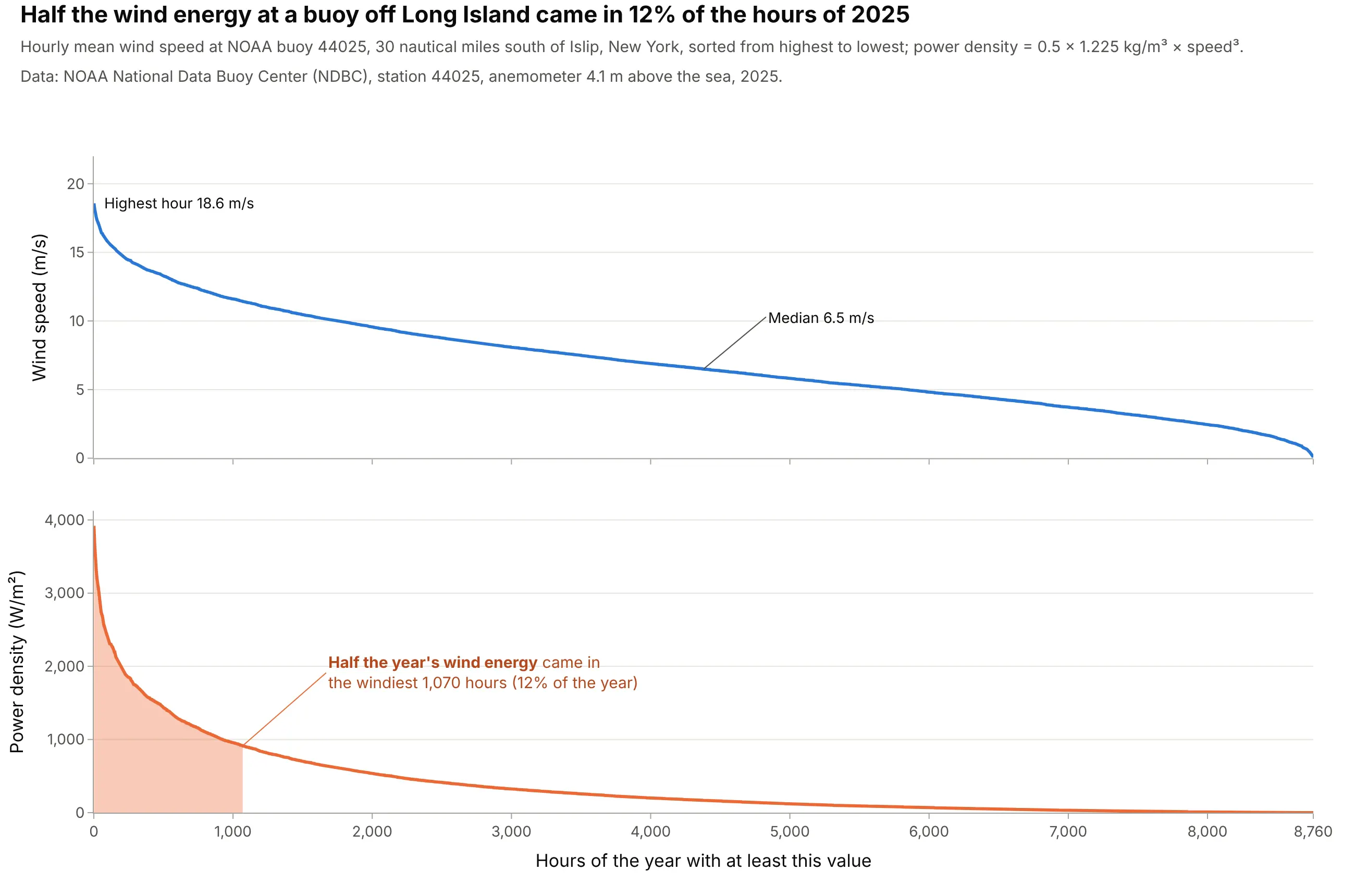
Two panels for NOAA buoy 44025 south of Long Island in 2025: hourly mean wind speed sorted from 18.6 m/s down to near zero with a median of 6.5 m/s, and below it wind power density, 0.5 times air density times speed cubed, from about 3,900 W/m² down to zero, with the first 1,070 hours shaded as half the year's wind energy

Any sensor log can be sorted the same way. At National Oceanic and Atmospheric Administration (NOAA) buoy 44025, 30 nautical miles south of Islip, New York, the median hourly wind speed in 2025 was 6.5 meters per second (m/s). Because the power in the wind grows with the cube of speed, half the year's wind energy came in the windiest 1,070 hours, 12% of the year. Data: NOAA National Data Buoy Center (NDBC), station 44025, anemometer 4.1 m above the sea, so speeds are lower than at a turbine's hub height.

Tip: put the measured value and a quantity derived from it on two panels with a shared x axis, so the same hour lines up in both.

Get the data from NOAA's National Data Buoy Center (ndbc.noaa.gov, station 44025, historical standard meteorological
data for 2025: 10-minute wind speed WSPD in m/s, 99.0 = missing) and average it to hours (columns: hour_utc,
wind_speed).

Build plotly subplots sharing the x axis: the wind speed duration curve on top and the power density duration
curve (0.5 x 1.225 x speed^3, W/m2) below, with the hours holding half the year's energy shaded.