Yield Curves - A Complete Guide

TL;DR

• A yield curve plots the interest rate (yield) on bonds from the same borrower against how long they run (their maturity), usually US Treasury bonds from 1 month to 30 years, so you can see in one line what it costs to borrow for every length of time.
• Yield curves are also known as the term structure of interest rates, Treasury yield curves, and par yield curves, and are similar to line charts. Their history through time is drawn as a heatmap or a 3D surface.
• The shape is the message: a normal curve slopes up, a flat curve says short and long rates are equal, and an inverted curve, with short rates above long ones, has come before each of the last six US recessions, but not always: the 2022-2024 inversion has had no recession after it as of October 2026.
• You can make a yield curve with Plotly from px.line or go.Scatter with maturities on a category or log axis, add animation_frame to play it over dates, and use go.Heatmap or go.Surface for decades of curves.

What is a yield curve?

Yield curves look like this:

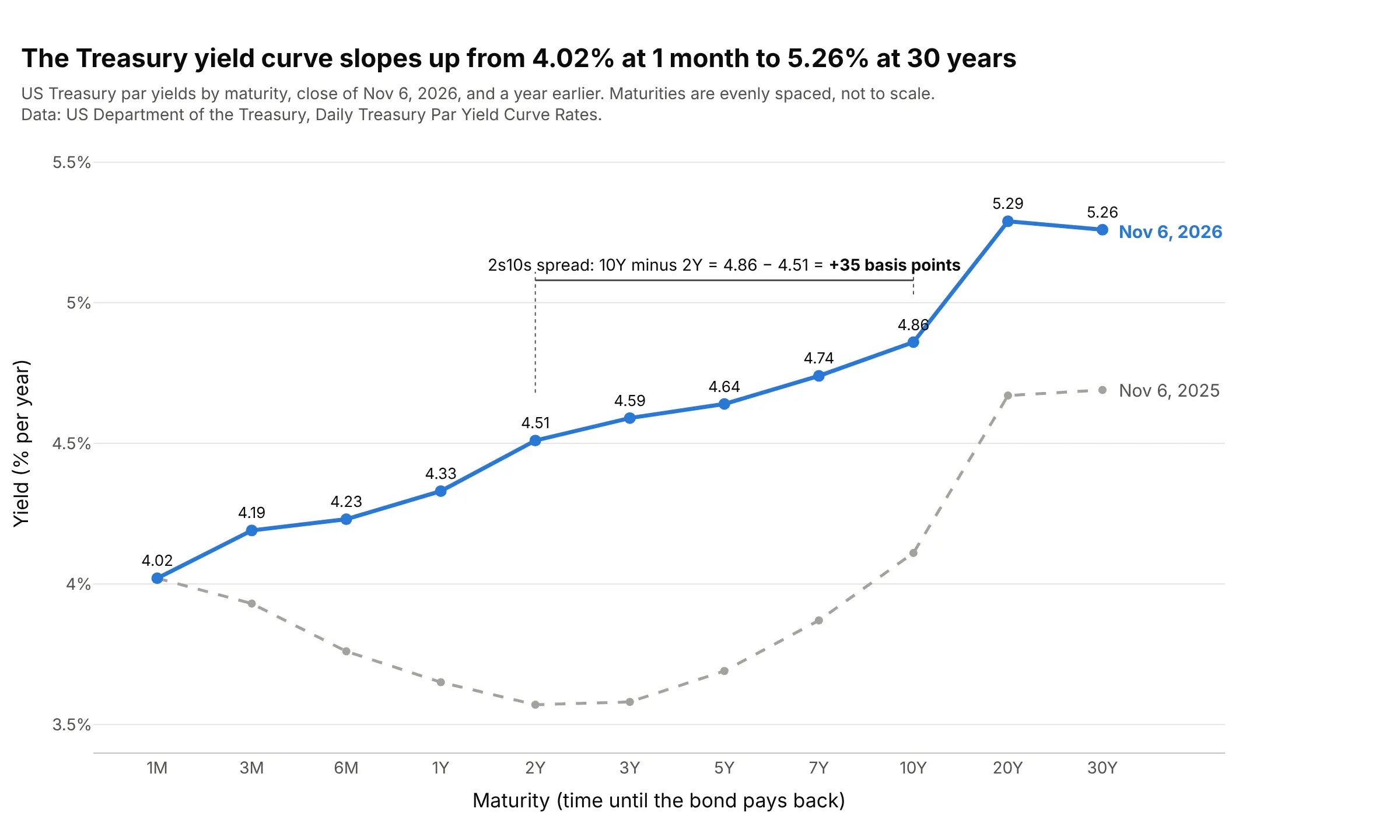
Data: US Department of the Treasury, Daily Treasury Par Yield Curve Rates.

How do you read a yield curve? In the example above, notice these things:

• Each point is the yield, in percent per year, that the US government paid to borrow for one length of time on November 6, 2026, from 1 month (1M) on the left to 30 years (30Y) on the right. The maturities are evenly spaced, so the axis is not to scale.
• The blue curve slopes up, from 4.02% at 1 month to 5.26% at 30 years. That is the normal shape: lenders usually ask for more to tie their money up for longer.
• The bracket marks the 2s10s spread, the 10-year yield minus the 2-year yield: 4.86 minus 4.51 is +35 basis points (bp), where 1 bp is 0.01 percentage point. This one number is the most quoted summary of the slope.
• The gray curve, a year earlier, dipped from 4.02% at 1 month to 3.57% at 2 years before rising, so short rates were above medium ones. Since then the 10-year rose 0.75 points and the 2-year 0.94.
• The 20-year yields a little more than the 30-year (5.29% against 5.26%), which has been true on 62% of days since June 2020, so a curve doesn't have to rise at every step.

It's often used for charts like these:

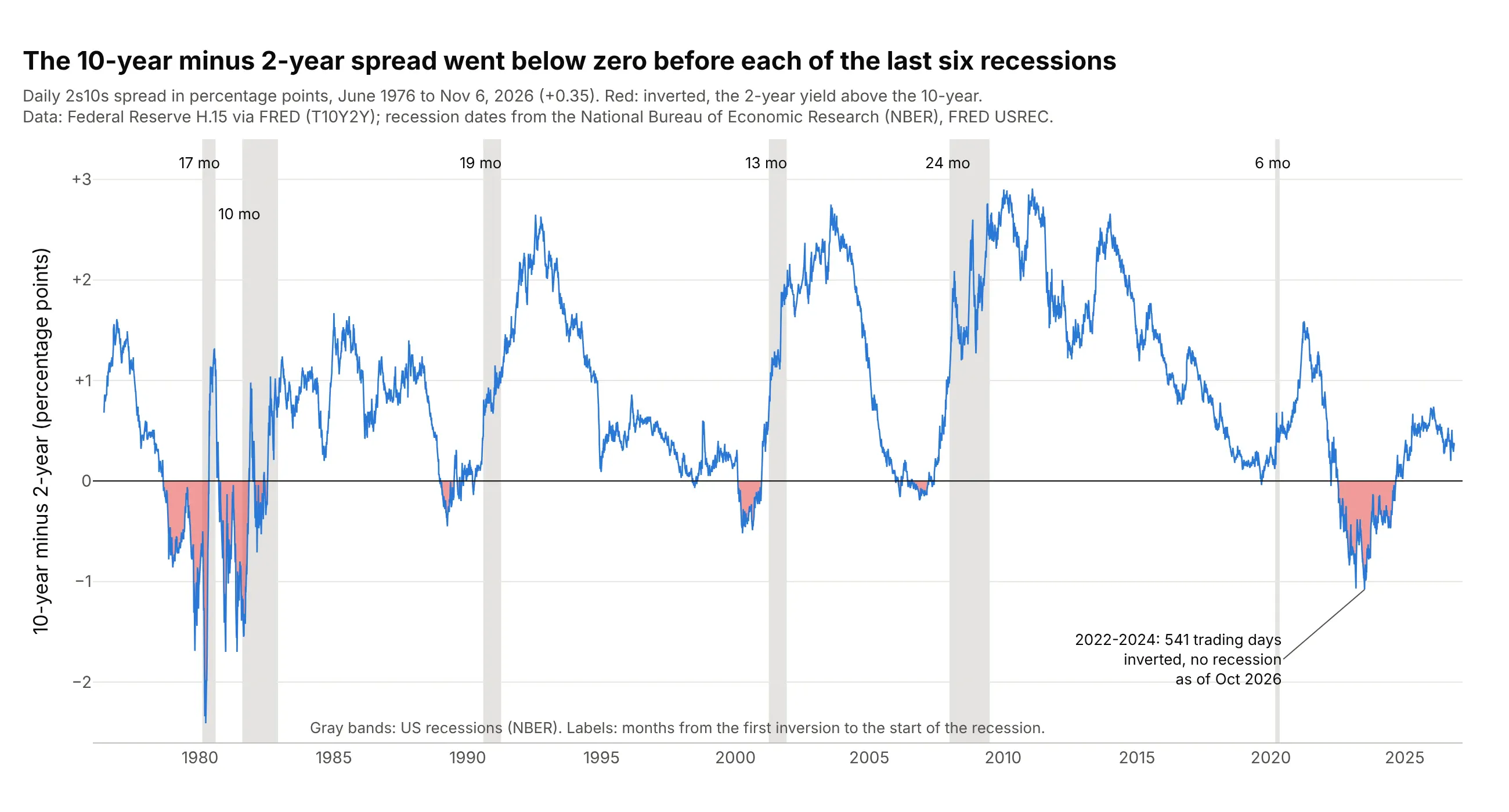
Watching for recessions. The 2s10s spread went below zero 6 to 24 months before each of the six recessions since 1976, which is why economists track it. Data: Federal Reserve H.15 release via FRED (Federal Reserve Economic Data, series T10Y2Y); recession dates from the National Bureau of Economic Research (NBER), FRED USREC.

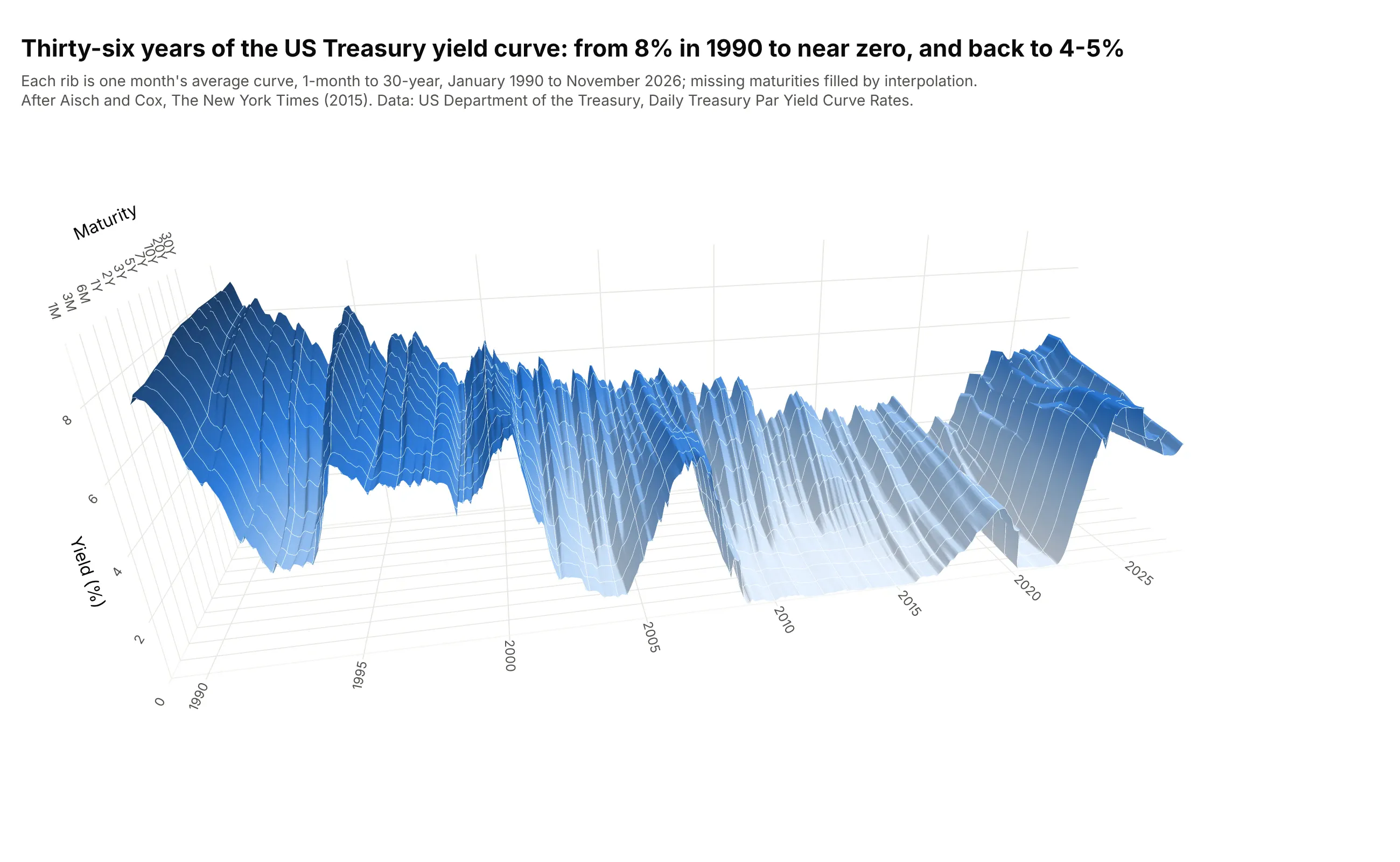
Showing decades of curves at once. Each of 443 monthly curves becomes one rib of a surface, the view Gregor Aisch and Amanda Cox drew for The New York Times in 2015. Data: US Treasury, Daily Treasury Par Yield Curve Rates, monthly averages.

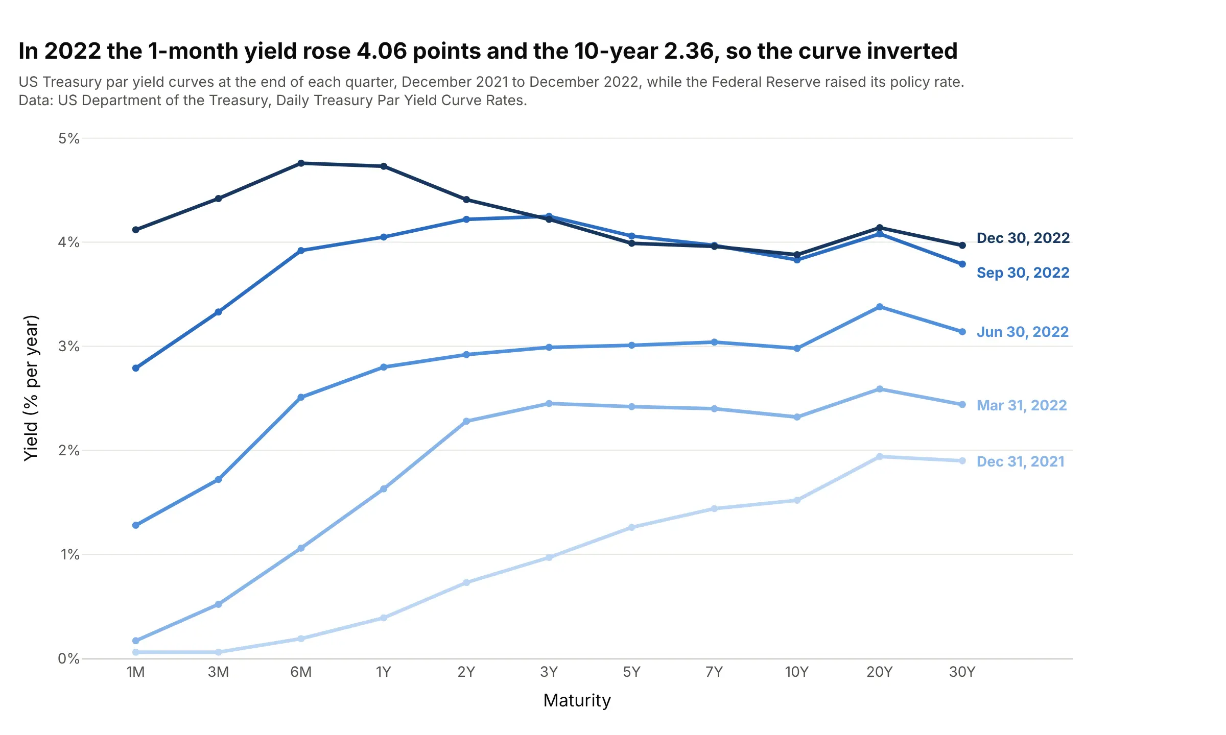
Comparing dates on a bond desk. Overlaying curves from several dates shows which maturities moved: in 2022 the 1-month yield rose 4.06 points and the 10-year 2.36, so the curve inverted. Data: US Treasury, Daily Treasury Par Yield Curve Rates.

A short history

In 1942 the National Bureau of Economic Research (NBER) published David Durand's "basic yield curves" for high-grade US corporate bonds, one for the first quarter of each year from 1900 to 1942 (Durand 1942). Durand plotted each bond's yield against its years to maturity and drew the curve by hand through the lowest yields, and his 1947 follow-up with Willis Winn tabulated the curves for 1943 to 1947 (Durand and Winn 1947). Here are those curves redrawn from their Table 1:

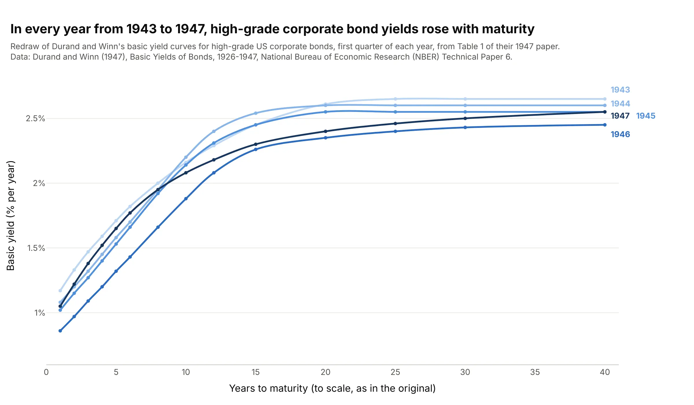
Data: Durand and Winn (1947), Basic Yields of Bonds, 1926-1947, NBER Technical Paper 6, Table 1 (redrawn with Plotly).

The link to recessions came later. Campbell Harvey's 1986 University of Chicago dissertation linked the slope of the curve to future consumption growth (Harvey 1988), and Estrella and Hardouvelis (1991) and Estrella and Mishkin (1998) tested the gap between long and short rates as a predictor of real activity and of recessions. In 2015 Gregor Aisch and Amanda Cox turned decades of daily Treasury curves into an interactive 3D chart for The Upshot (The New York Times), and FlowingData called it a fine exception to the usual case against 3D charts.

Yields, maturities, and the maturity axis

A bond is a loan you can buy and sell: the borrower pays interest and returns the money on a set date, its maturity. The yield is the return per year you get if you buy the bond at today's price and hold it to maturity, so it moves the opposite way to the price. The US Treasury borrows at every maturity from 1 month (bills) to 30 years (bonds), and because the borrower is the same, the only difference between the points on its curve is time.

The Treasury publishes its curve every business day from bid prices of the most recently auctioned securities, taken at about 3:30 PM, and fits a smooth curve through them (a monotone convex interpolation since December 6, 2021, according to its methodology page). The yields are par yields, the coupon at which a new bond of that maturity would sell for exactly its face value. Other curves you will meet are spot (zero-coupon) curves, used by the European Central Bank and by pension actuaries, and forward curves.

The maturities are the awkward part. Of the Treasury's 14 published maturities, 8 are under 3 years, so the axis needs a decision. These are the same 14 yields on three axes:

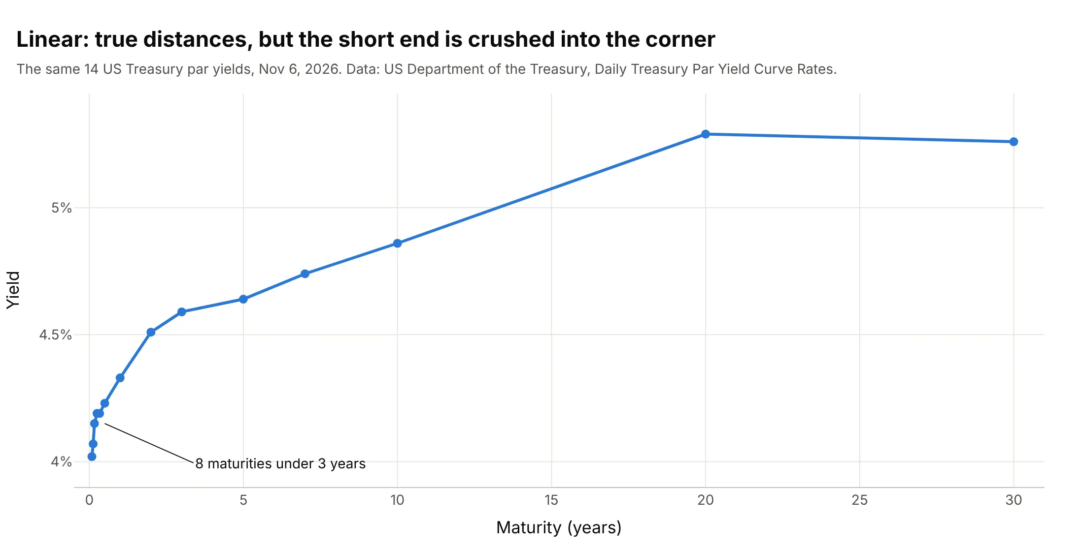
Linear axis (true distances). The 20 years between 10Y and 30Y get two thirds of the width, and the short end, where central bank policy shows up first, is crushed into a corner. Use it when distance in years matters, as in the corporate bond example below.

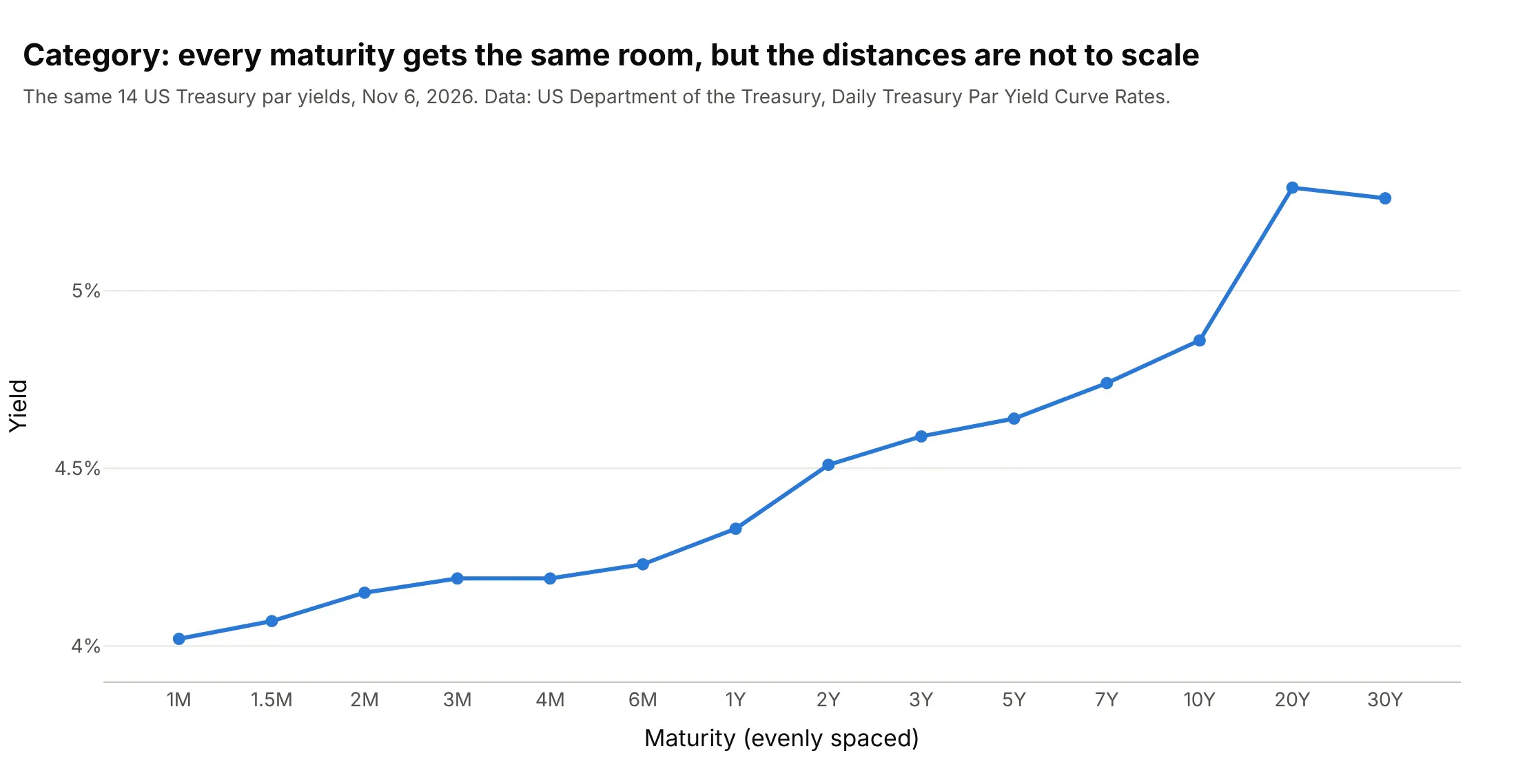
Category axis (evenly spaced). Every published maturity gets the same room, in the order the Treasury lists them in its tables. The cost is that 1M to 2M looks as long as 20Y to 30Y, so say "not to scale" in the subtitle.

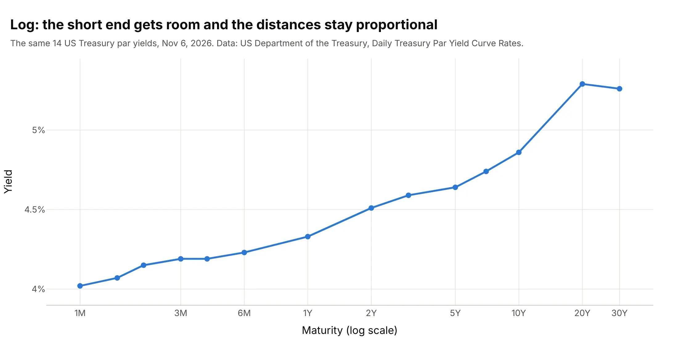
Log axis (proportional). Each doubling of maturity gets the same width, so the short end has room and the gaps stay honest. It is the best choice when curves from different sources use different maturities, as in the US, euro area, and Japan example below.

Normal, flat, inverted, and humped yield curves

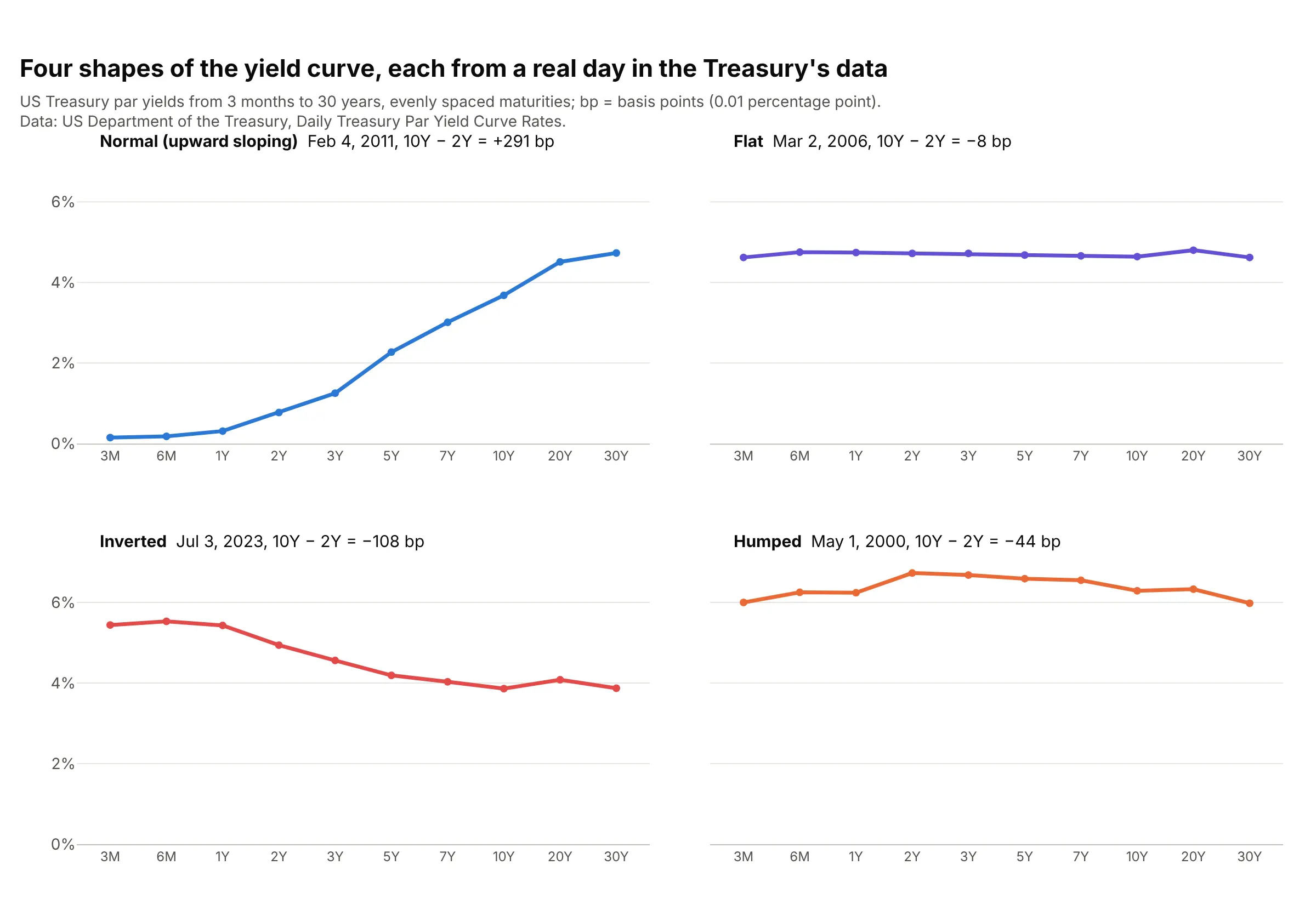
Lenders usually want a higher yield to lend for longer, because more can go wrong with inflation and interest rates over 30 years than over 3 months, and that extra return is called the term premium. Long yields also carry what investors expect short rates to do in the future, so the shape of the curve says something about where people think the central bank's rate is headed. These four days are the most extreme examples of each shape in the Treasury data since 1990:

Data: US Treasury, Daily Treasury Par Yield Curve Rates.

• Normal (upward sloping). Short rates are low and investors expect them to rise, as in February 2011, when the 3-month bill yielded 0.15% and the 30-year bond 4.73%. The 2s10s spread was +291 bp, the largest since 1990.
• Flat. Short and long yields are about equal, as in March 2006, when every maturity was between 4.62% and 4.80%. Investors expect short rates to stay about where they are, and lending for 30 years pays no more than lending for 3 months.
• Inverted. Short yields are above long ones, as on July 3, 2023, when the 6-month yielded 5.53% and the 10-year 3.86%. It means investors expect short rates to fall, typically after the central bank has raised them and when they expect the economy to slow.
• Humped. Medium maturities yield more than both ends, as in May 2000, when the 2-year was at 6.73% and the 3-month and 30-year near 6%.

The 2s10s spread and recessions

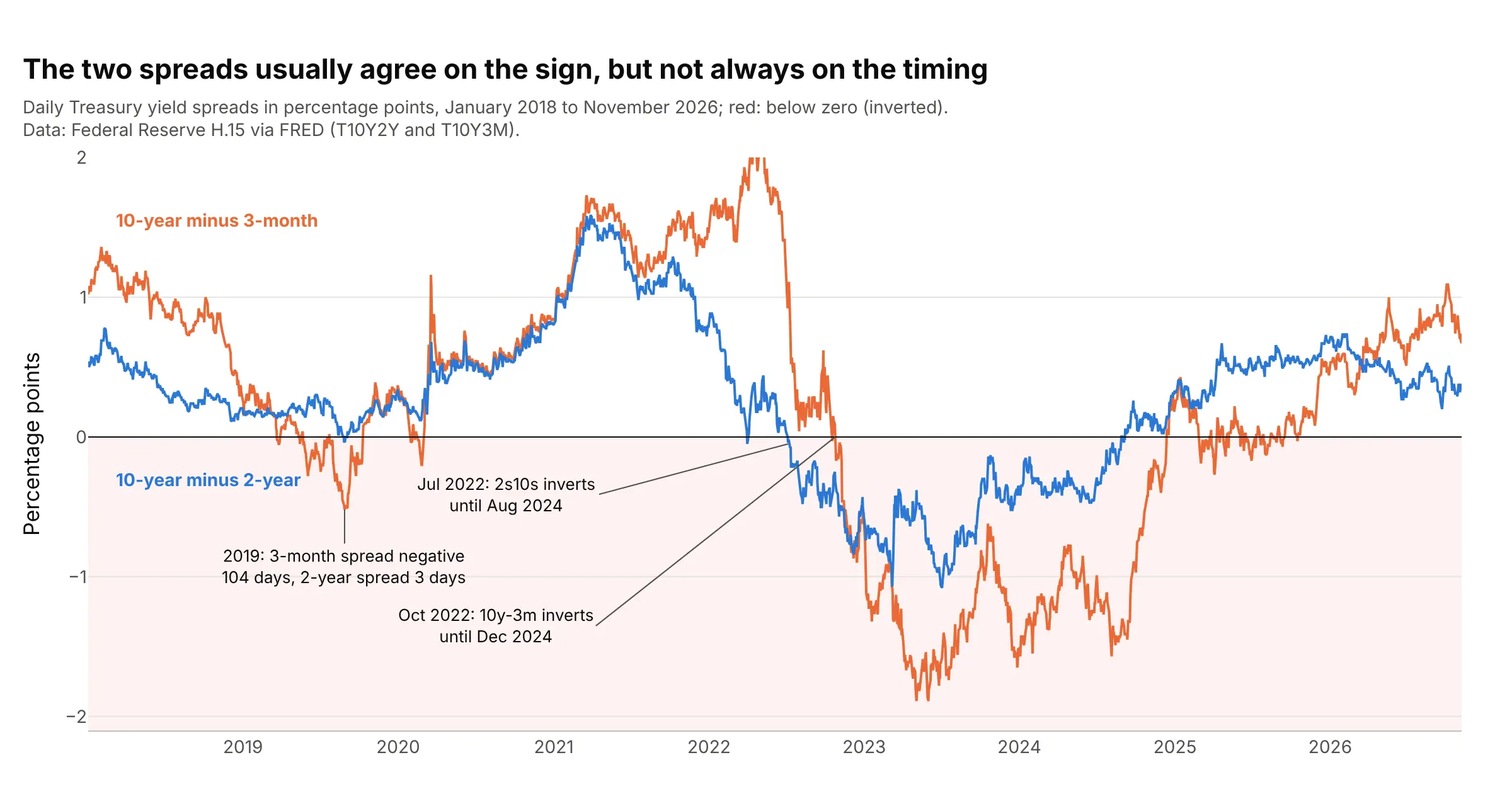
Bond traders name spreads by their two maturities: "2s10s" is the 10-year yield minus the 2-year, and "10y-3m" is the 10-year minus the 3-month. A negative value means the curve is inverted between those two points. The Federal Reserve Bank of New York (the New York Fed) uses the 10-year minus 3-month spread, which its economists found "provides a reasonable combination of accuracy and robustness in predicting U.S. recessions", and noted that the 2s10s "tends to turn negative earlier and more frequently" (Estrella and Trubin 2006). The two usually agree on the sign but not on the timing:

Data: Federal Reserve H.15 via FRED (T10Y2Y and T10Y3M).

The record since 1976 is in the second chart of this guide. The 2s10s spread went below zero before each of the six recessions, between 6 and 24 months ahead, which is the record behind the common claim that an inversion comes before a recession. Three caveats come with it:

• The lead time varies. It was 17 months before the 1980 recession, 10 before 1981, 19 before 1990, 13 before 2001, 24 before 2007, and 6 before 2020, so an inversion doesn't say when.
• Some inversions had no recession after them. The 2s10s was briefly negative in mid-1998, and from July 2022 to August 2024 it stayed below zero for the longest stretch in the data, reaching -1.08 on July 3, 2023, the most negative since 1981. The NBER had dated no recession after it as of October 2026.
• The 2020 signal was weak. The 2s10s was negative on only 3 days in August 2019 (the 10y-3m on 104 days), and the 2020 recession was set off by the COVID-19 pandemic.

The New York Fed turns the 10-year minus 3-month spread into a probability of a recession twelve months ahead, shown in example 9 below, and as of November 2026 it puts that probability at 12.4% for October 2027.

Alternatives to a yield curve

Here's the same set of Treasury curves, January 2019 to November 2026, drawn six ways. Some are better for the question, some worse, some just different:

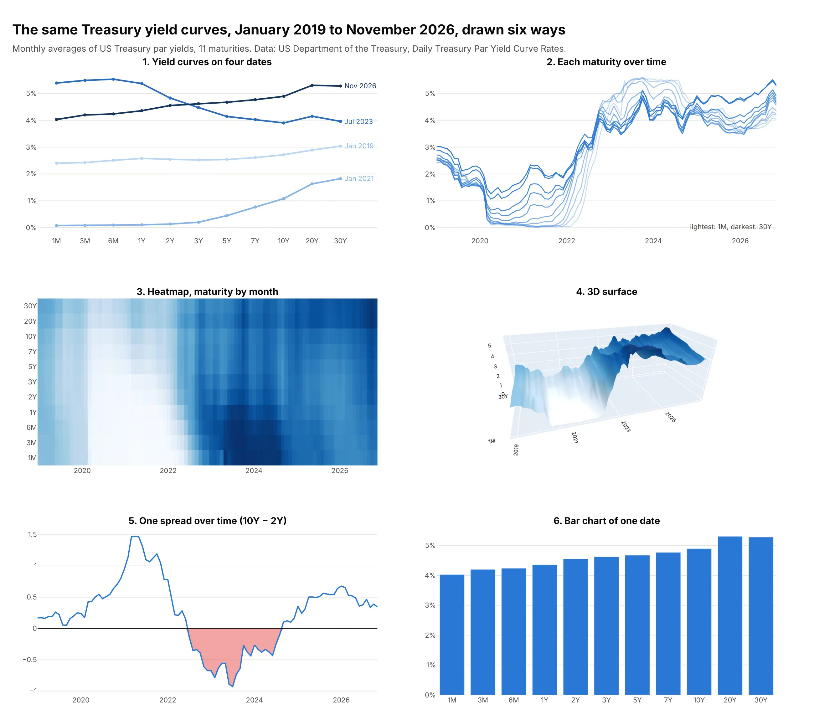
• Yield curves on a few dates (the chart itself). The shape on each date is readable, and two to five dates compare well, much like a before-and-after slope chart. Beyond about five dates the lines tangle.
• Each maturity over time (different). A line chart of yields by date answers "how did the 10-year move?" better, but the shape of the curve on any one day disappears among 11 lines.
• Heatmap (better for decades). Every month and maturity is visible at once with no hidden areas, and a diverging color scale on the spread to the 10-year makes inversions stand out (example 3 below). Reading exact values needs hover.
• 3D surface (works too, for the big picture). The surface shows the decades-long fall and rise of rates and is memorable, which is why the New York Times used it, but parts of it hide others and exact values are hard to read from a static image.
• One spread over time (better for the recession question). The 2s10s or 10y-3m spread as a line, with zero marked, answers "is it inverted?" precisely, but it reduces the whole curve to one number.
• Bar chart of one date (worse). Bars start at zero, so the differences between 4.0% and 5.3% look small, and bars break the idea of a continuous curve. Bars do work for the change in yield by maturity (example 2 below).

How to make a yield curve

With AI

ChatGPT, Claude Code, GitHub Copilot, Cursor, and other AI tools are excellent at writing Plotly code. Name Plotly in the prompt, and say how the maturities should be spaced and which dates to compare:

With Plotly Studio

Plotly Studio is a desktop app where you point an AI at a dataset and it builds charts and a Dash app around your questions. Ask for a yield curve the same way:

Show the Treasury yield curve for a date I pick, with maturities evenly spaced from 1M to 30Y, a second date to compare as a dashed line, the 10-year minus 2-year spread below it as a line over time with inversions in red, and a slider to play the curve week by week.

Make a yield curve in Python or JavaScript

This is the code AI tools write under the hood. In Python, px.line draws the curves straight from the Treasury's CSV, one line per date. The category_orders argument matters: without it the maturities would be sorted as text ("1 Mo", "1 Yr", "10 Yr", "2 Yr", ...):

To play the curve over dates, pass animation_frame="Date" instead of color and set range_y, because the axes don't rescale between frames (the line chart guide animates month-end curves this way, and example 1 below does it week by week). For a log axis, use the maturity in years as x and fig.update_xaxes(type="log"). For decades of curves, pivot to a grid of dates by maturities and pass it as z to go.Heatmap or go.Surface.

In JavaScript, plotly.js draws the same chart with one scatter trace per date on a category axis:

Share it

Every Plotly chart has a Share chart button (the cloud icon in its toolbar) that uploads it to Plotly Cloud and gives you a link. Only you can see it until you change its visibility.

For a live app, put the chart in a Dash app and publish it with the Plotly Cloud CLI. Coding agents can run these commands for you:

If your data has to stay in your own cloud or data center, publish to Dash Enterprise instead.

Dos and don'ts

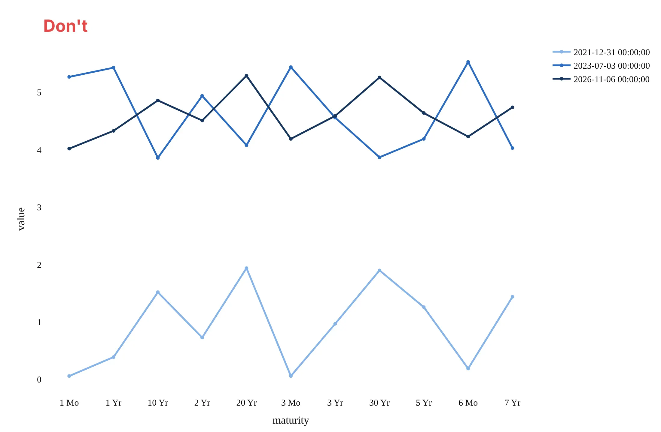
Most mistakes in published yield curves come from the maturity column, which arrives as text, and from comparing dates without saying which is which. Here are three Treasury curves both ways, in the same blues.

Don't let the maturities sort as text, which puts 10 Yr before 2 Yr and scrambles every curve into a zigzag, leave the legend as raw timestamps, drop the percent unit, or keep a serif font and raw column names:

Do keep the maturities in order from shortest to longest, label each curve with its date at the end of the line, show yields in percent, and use a sequential color, light for older and dark for newer:

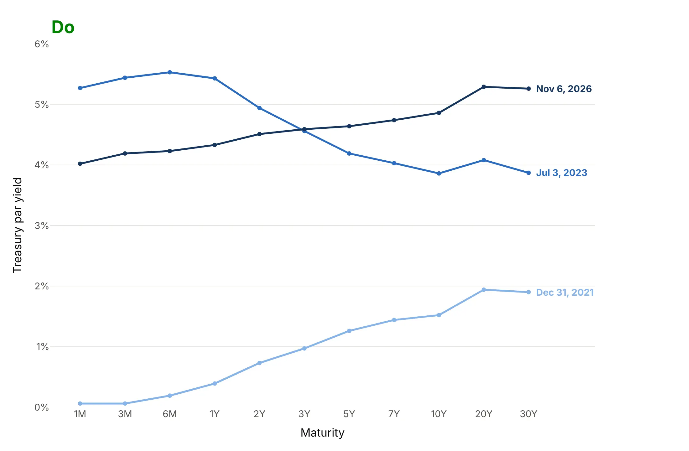
Checklist

Do

• Order maturities by length and say whether the axis is evenly spaced, log, or to scale.
• Put the date of every curve on the chart, and the time of day if you compare intraday curves.
• Quote spreads in basis points and say which two maturities (2s10s, 10y-3m).
• Use the same y range when you compare charts or animation frames.
• Say which curve you plot (par, spot, or forward), because they differ by up to tens of basis points.
• Shade recessions from an official source (NBER in the US) when you plot a spread over time.

Don't

• Mix par yields and spot yields on one chart without saying so.
• Draw a curve through maturities that weren't published on that date without marking the gap or the interpolation.
• Describe an inversion as a forecast of a recession on a date; the lead time has ranged from 6 to 24 months.
• Use bars for yield levels; use them for changes.

Options to customize

A yield curve in Plotly is a go.Scatter trace on a category or log axis, and its history is a heatmap or a surface, so these are the options that matter most. The full lists are in the scatter trace reference, the axes documentation, and the animations documentation.

1. xaxis.type="category" with categoryorder="array", categoryarray=[...] (or category_orders in Plotly Express): evenly spaced maturities in the right order.
2. xaxis.type="log" with tickvals and ticktext: proportional spacing, labeled 1M, 3M, 1Y, 10Y, 30Y.
3. mode="lines+markers+text" with texttemplate: the yield printed at each maturity.
4. line.dash and a muted line.color: an earlier date as a reference curve.
5. fig.add_annotation(xanchor="left", xshift=...): direct labels at the end of each curve instead of a legend.
6. animation_frame and range_y in px.line: one frame per date with fixed axes.
7. fill="tozeroy" on a clipped copy of the spread: inversions filled red below zero.
8. fig.add_vrect: recession bands behind a spread chart.
9. go.Heatmap(zmid=0) with a diverging colorscale: spreads by maturity and date, inversions in red.
10. go.Surface with scene.aspectratio and scene.camera.eye: the 3D view of curves through time.

More yield curve examples

Nine more yield curve charts built from real public data, each with its source, the technique that makes it work, and a prompt to rebuild it. They go deeper than the line chart guide's animation, into changes, heatmaps, other markets, and the models that analysts fit to the curve.

1. Week by week through the 2022-2023 rate hikes

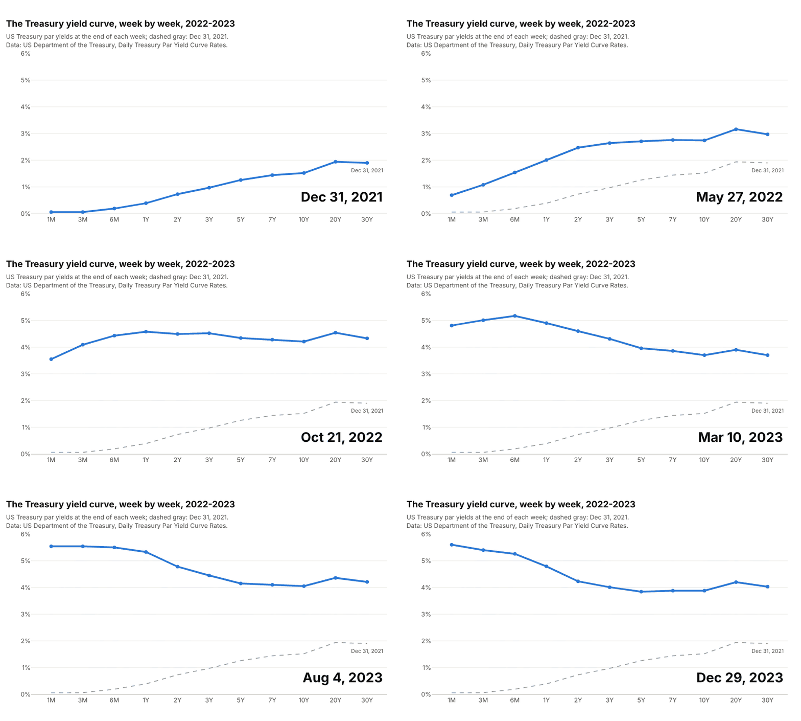
The curve moved from steep to inverted in about six months of 2022, short end first, and stayed inverted for the rest of the animation's 105 weeks. Data: US Treasury, Daily Treasury Par Yield Curve Rates, last business day of each week.

Tip: keep a gray copy of the first frame on every frame, so viewers see how far the curve has moved.

2. What moved after the Federal Reserve started cutting

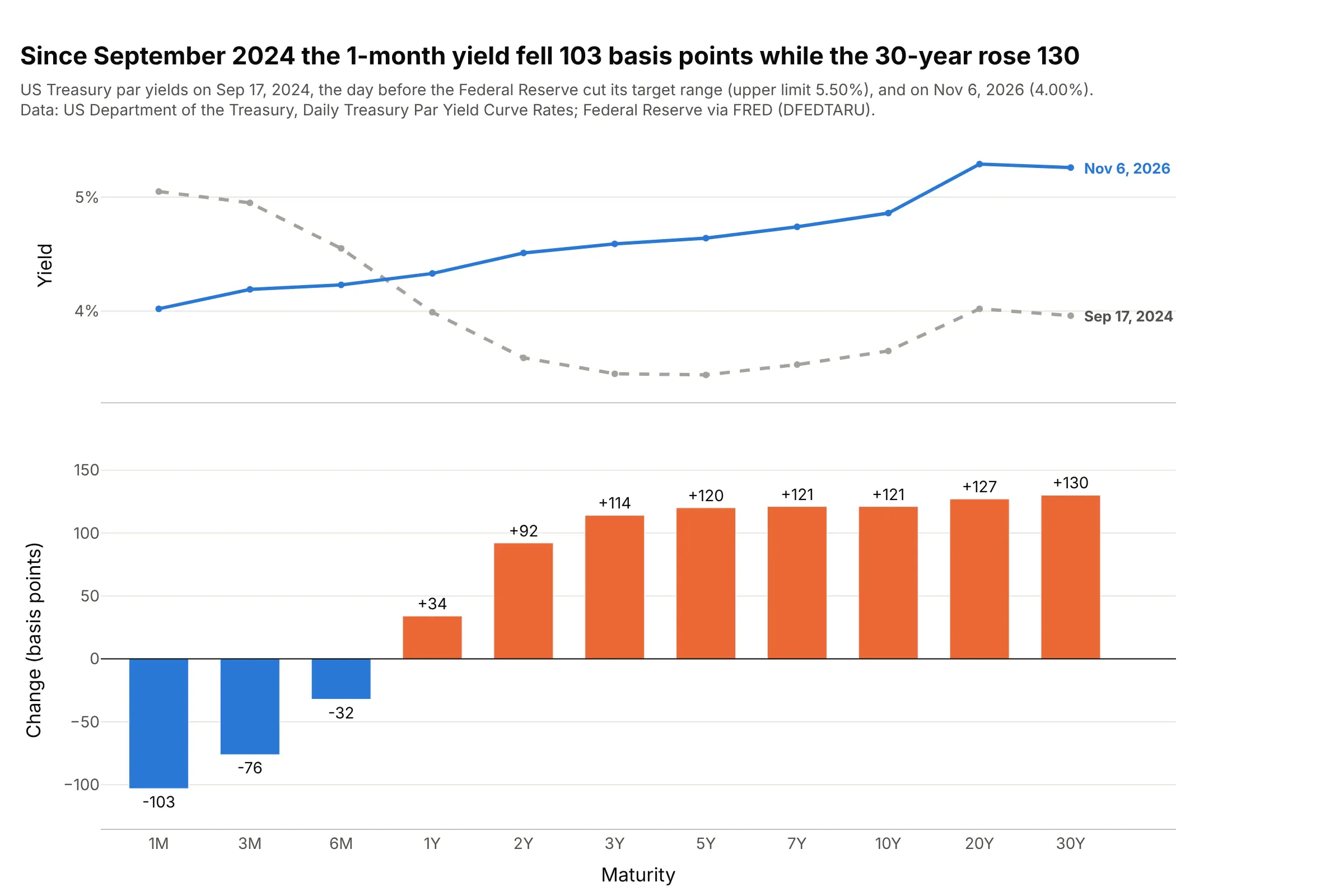
From the day before the Federal Reserve's first cut in September 2024 to November 6, 2026, the 1-month yield fell 103 bp while the 30-year rose 130, so the curve steepened from both ends. Data: US Treasury, Daily Treasury Par Yield Curve Rates; Federal Reserve via FRED (DFEDTARU).

Tip: when two curves cross, plot the change as bars, which is easier to read than the gap between two lines.

3. Every inversion since 1990 as a red band

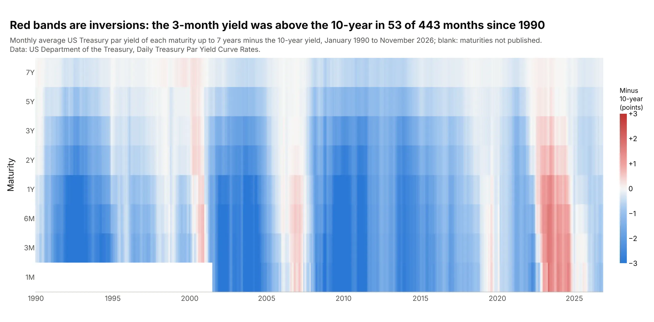
Subtracting the 10-year from each shorter maturity turns color into shape: the 3-month yield was above the 10-year in 53 of 443 months since 1990, and every such month shows red. Data: US Treasury, Daily Treasury Par Yield Curve Rates, monthly averages.

Tip: set zmid=0 on a diverging scale so white means flat and the colors mean the same thing in every month.

Another way to see it: the same data as the 3D surface in the "What is" section shows the level of rates, while the heatmap of spreads shows the shape. Use the surface for the story of rates and the heatmap to find every inversion.

4. Nominal, real, and the inflation priced in between

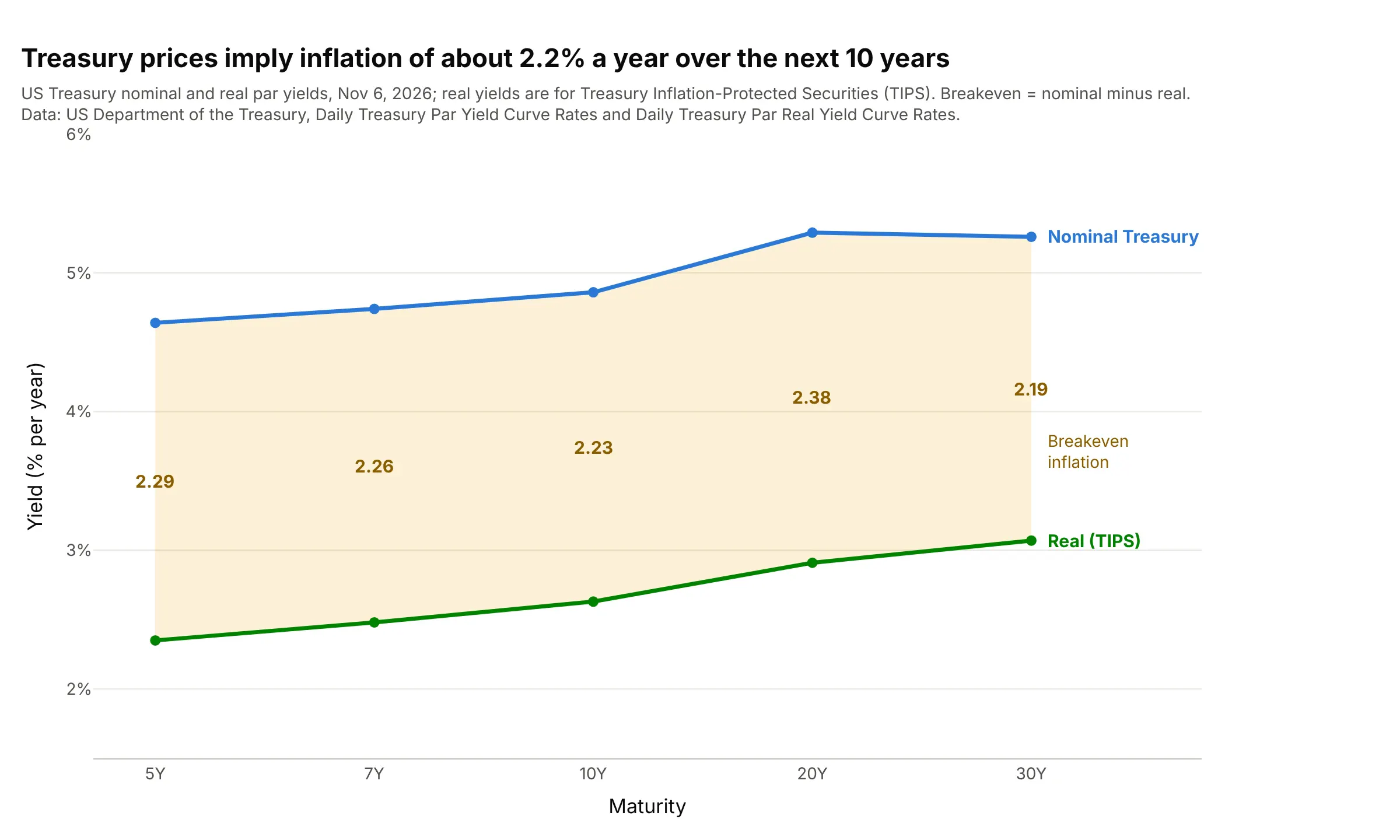
Treasury Inflation-Protected Securities (TIPS) pay a real yield on top of inflation, so the gap to the nominal curve is the inflation investors are paid for, about 2.2% a year over 10 years. That breakeven also contains a risk premium, so it is close to, not equal to, expected inflation. Data: US Treasury, Daily Treasury Par Yield Curve Rates and Daily Treasury Par Real Yield Curve Rates.

Tip: shade the band between two curves with fill="tonexty" and print the gap inside it.

5. The US, the euro area, and Japan on the same day

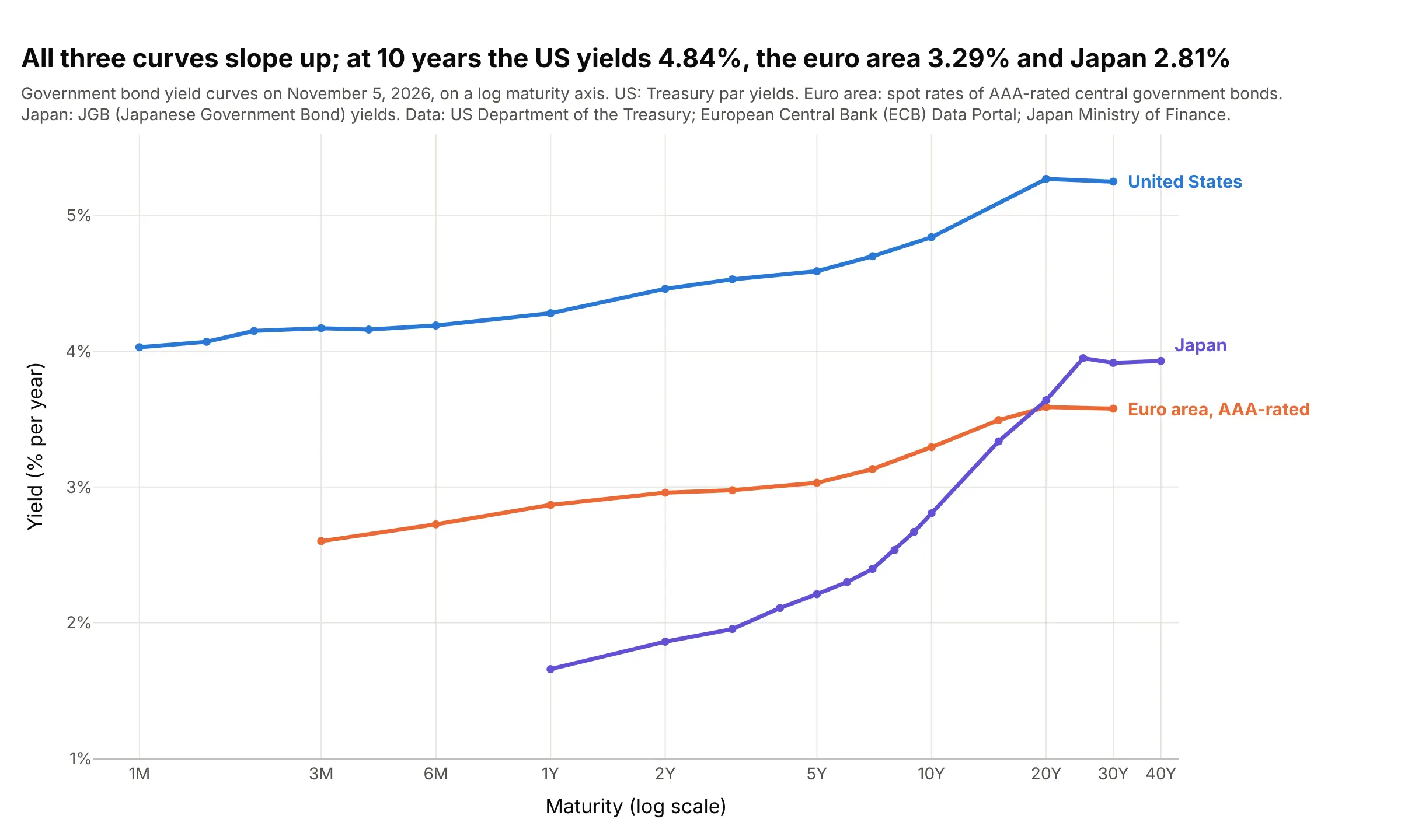
All three curves slope up, but at 10 years the US Treasury yielded 4.84%, euro area governments rated AAA (the top credit rating) 3.29% and Japan 2.81%, and Japan's curve rises the most steeply past 10 years. Data: US Treasury; European Central Bank (ECB) Data Portal, euro area yield curves; Japan Ministry of Finance, Japanese Government Bond (JGB) interest rates.

Tip: when sources publish different maturities, put years on a log axis instead of categories so every point lands in its true place.

6. What companies pay over the Treasury, by maturity

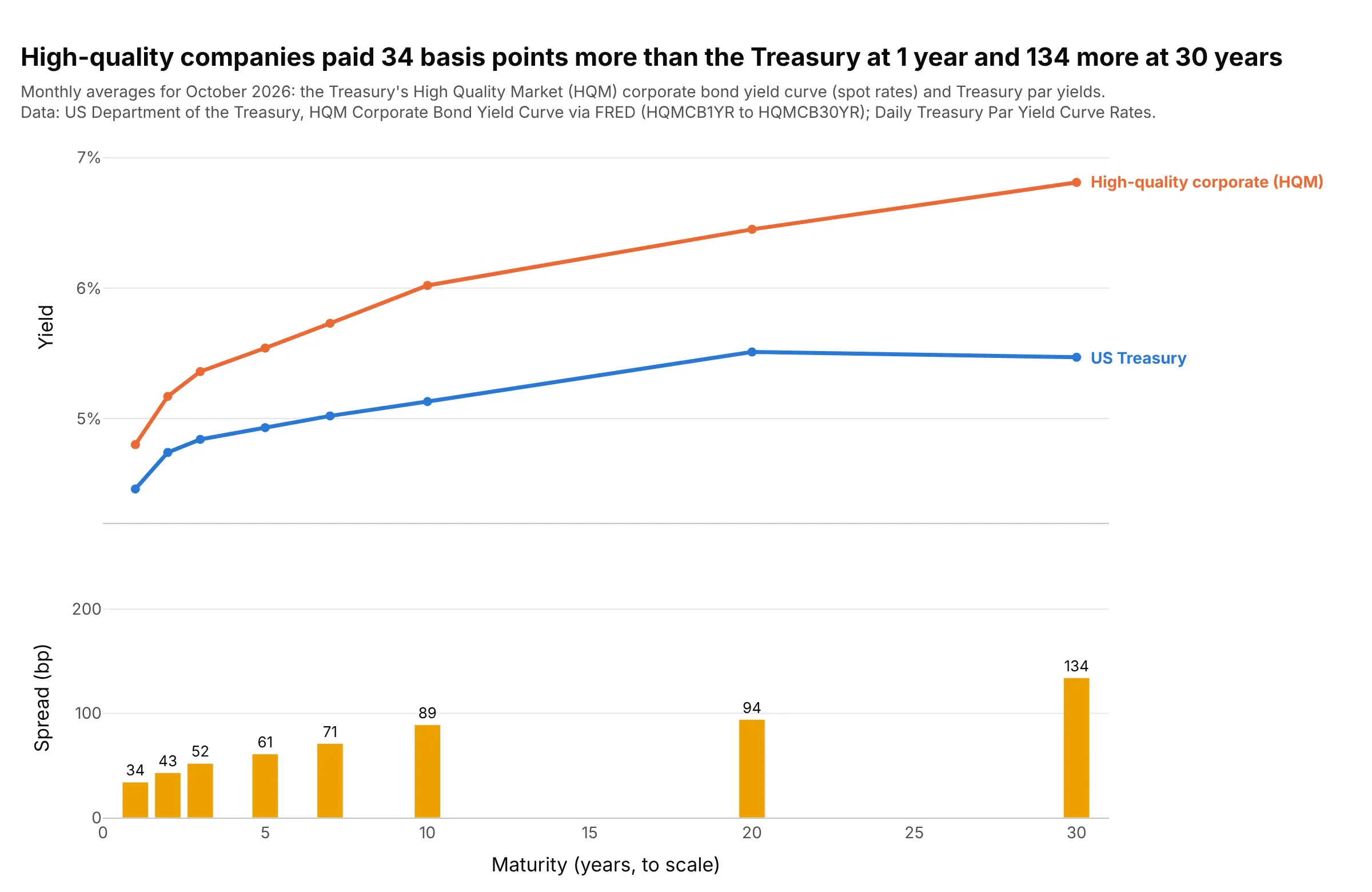
In October 2026 high-quality companies paid 34 bp more than the Treasury to borrow for 1 year and 134 bp more for 30 years. The Treasury publishes this High Quality Market (HQM) corporate curve for discounting pension obligations under the Pension Protection Act of 2006. Data: US Treasury HQM Corporate Bond Yield Curve via FRED; Daily Treasury Par Yield Curve Rates, monthly averages.

Tip: the HQM curve is a spot curve and the Treasury curve a par curve, so treat the gap as an approximate credit spread.

7. A smooth curve from 14 yields: the Nelson-Siegel model

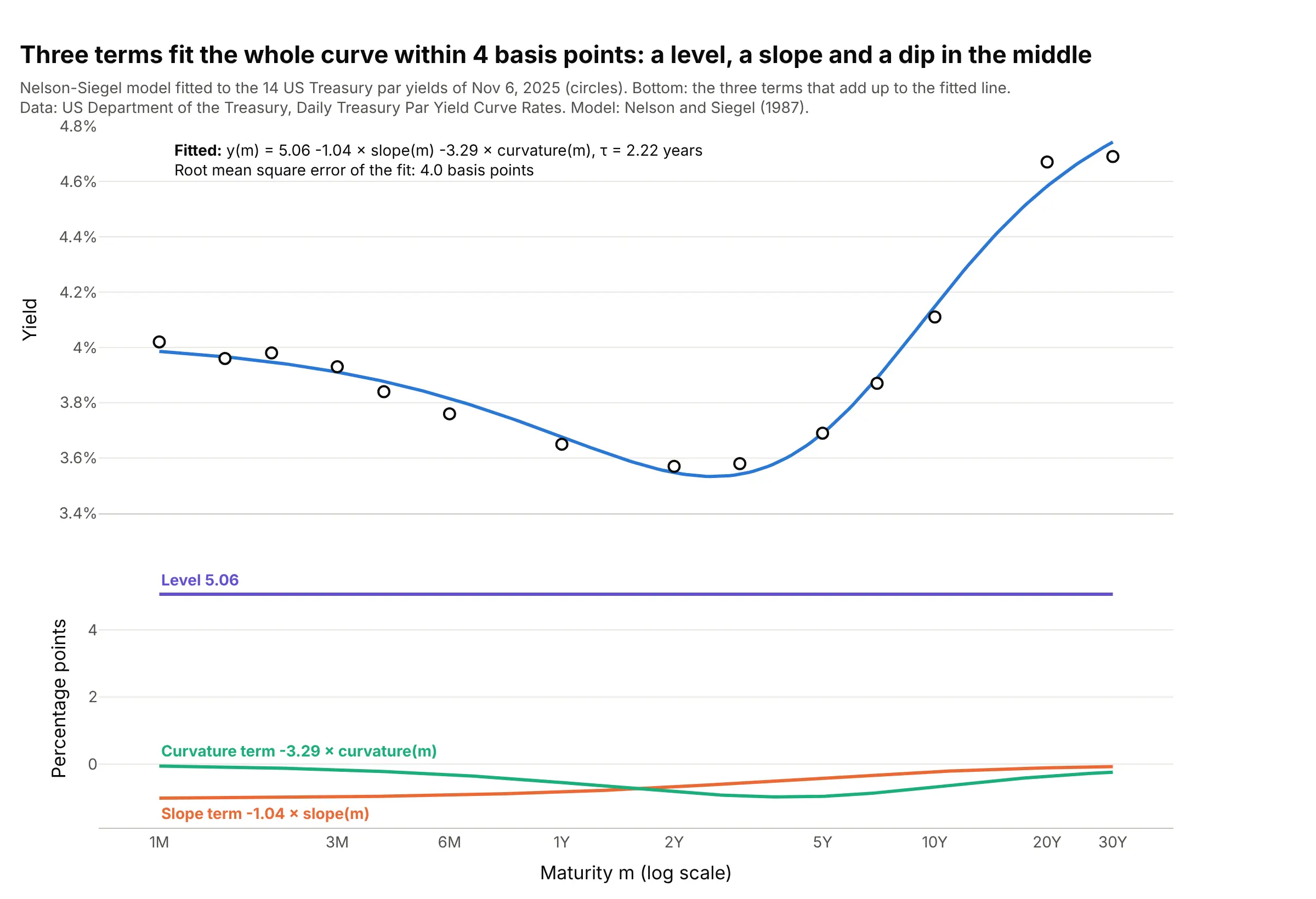
Nelson and Siegel (1987) describe a whole curve with a level, a slope that fades with maturity, and a hump, and on November 6, 2025 those three terms fit all 14 Treasury yields within 4 bp. Central banks such as the ECB use an extension of it for their published curves. Data: US Treasury, Daily Treasury Par Yield Curve Rates.

Tip: for a fixed decay parameter the model is linear, so search tau on a grid and solve the rest by least squares; it avoids the local minimums that a general optimizer can fall into.

8. Level, slope, and curvature in 20 years of daily moves

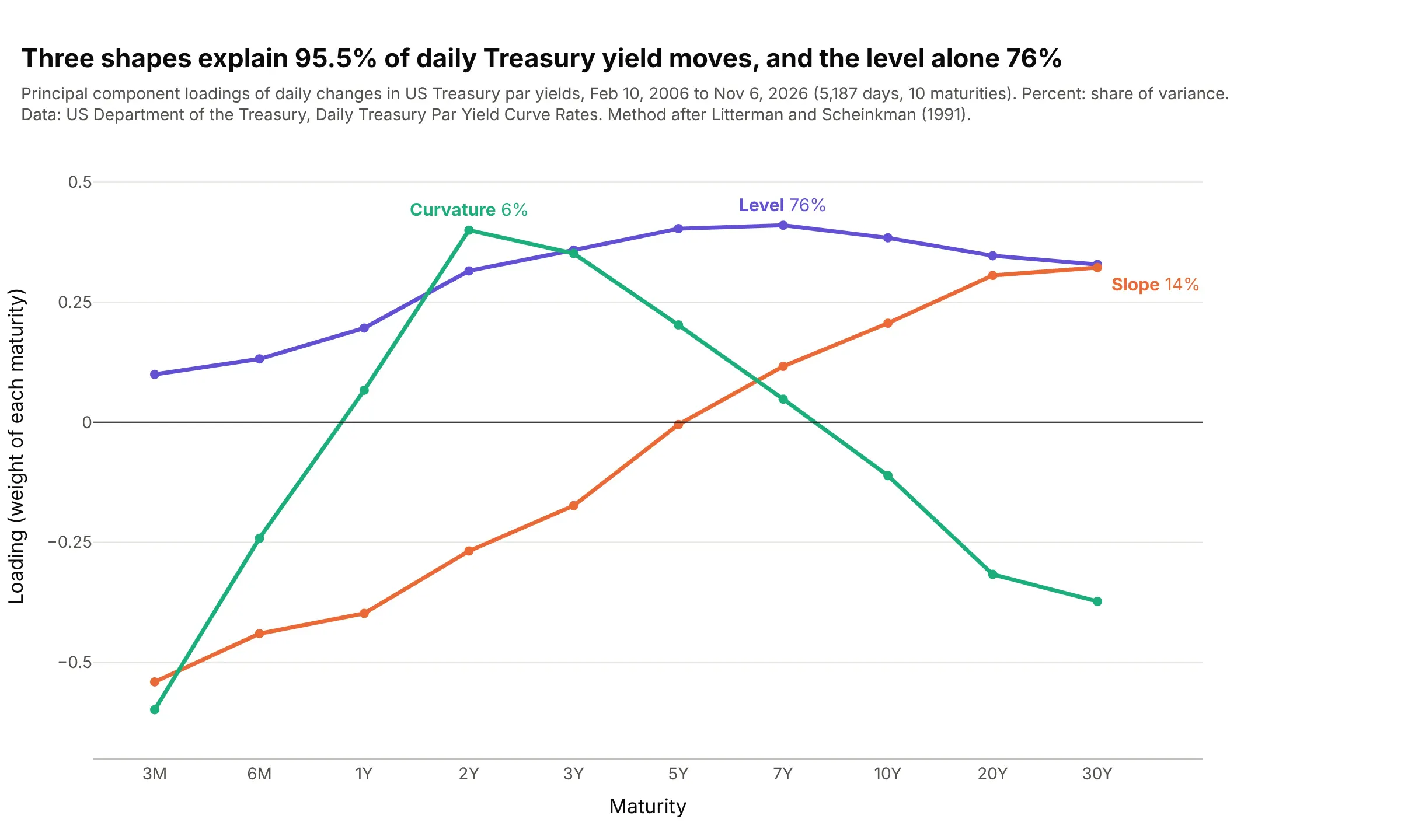
A principal component analysis (PCA) of 5,187 days of yield changes finds three shapes that explain 95.5% of the moves: the whole curve shifting (76%), the ends moving apart (14%) and the middle moving against both ends (6%). Litterman and Scheinkman (1991) described three common factors like these in Treasury returns. Data: US Treasury, Daily Treasury Par Yield Curve Rates, February 2006 to November 2026.

Tip: draw each component on the maturity axis, so it reads as a shape the curve can take.

9. The New York Fed's recession probability

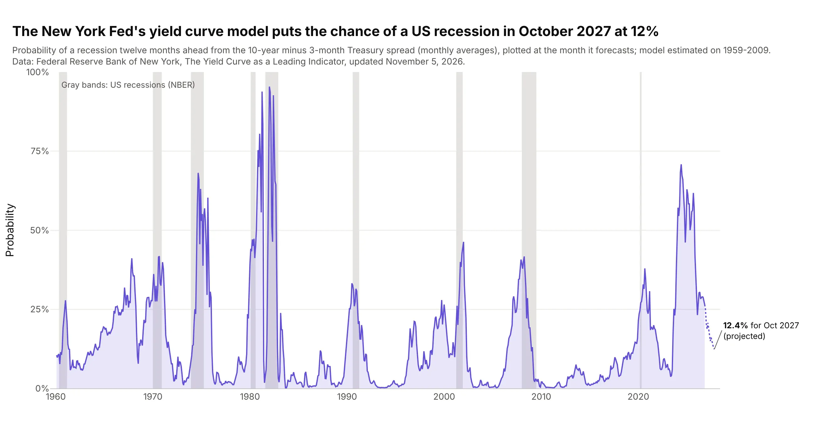
The Federal Reserve Bank of New York's model turns the 10-year minus 3-month spread into a probability of a US recession a year ahead, and it puts October 2027 at 12.4%, down from 70.9% for May 2024, a peak with no recession after it so far. Data: Federal Reserve Bank of New York, The Yield Curve as a Leading Indicator.

Tip: plot a forecast at the month it forecasts, not the month it was made, so it lines up with the recession bands.