Chris Parmer

October 24, 2026

Slope Charts - A Complete Guide

TL;DR

A slope chart draws one line per item between two or three columns, usually two dates, so the slope of each line is the change and the order at each end is the ranking.
Slope charts are also known as slopegraphs and slope graphs, and are similar to dumbbell charts and bump charts.
Use one for before-and-after comparisons of about 5 to 30 items when both the change and the reshuffle matter. Use a line chart when the path between the dates matters, and a dumbbell chart for more items or a narrow screen.
Label both ends directly, put one to three stories in color and the rest in gray, and nudge labels apart so close values stay readable.
You can make a slope chart with Plotly from go.Scatter lines and annotations, and any coding agent can write that for you in a minute.

What is a slope chart?

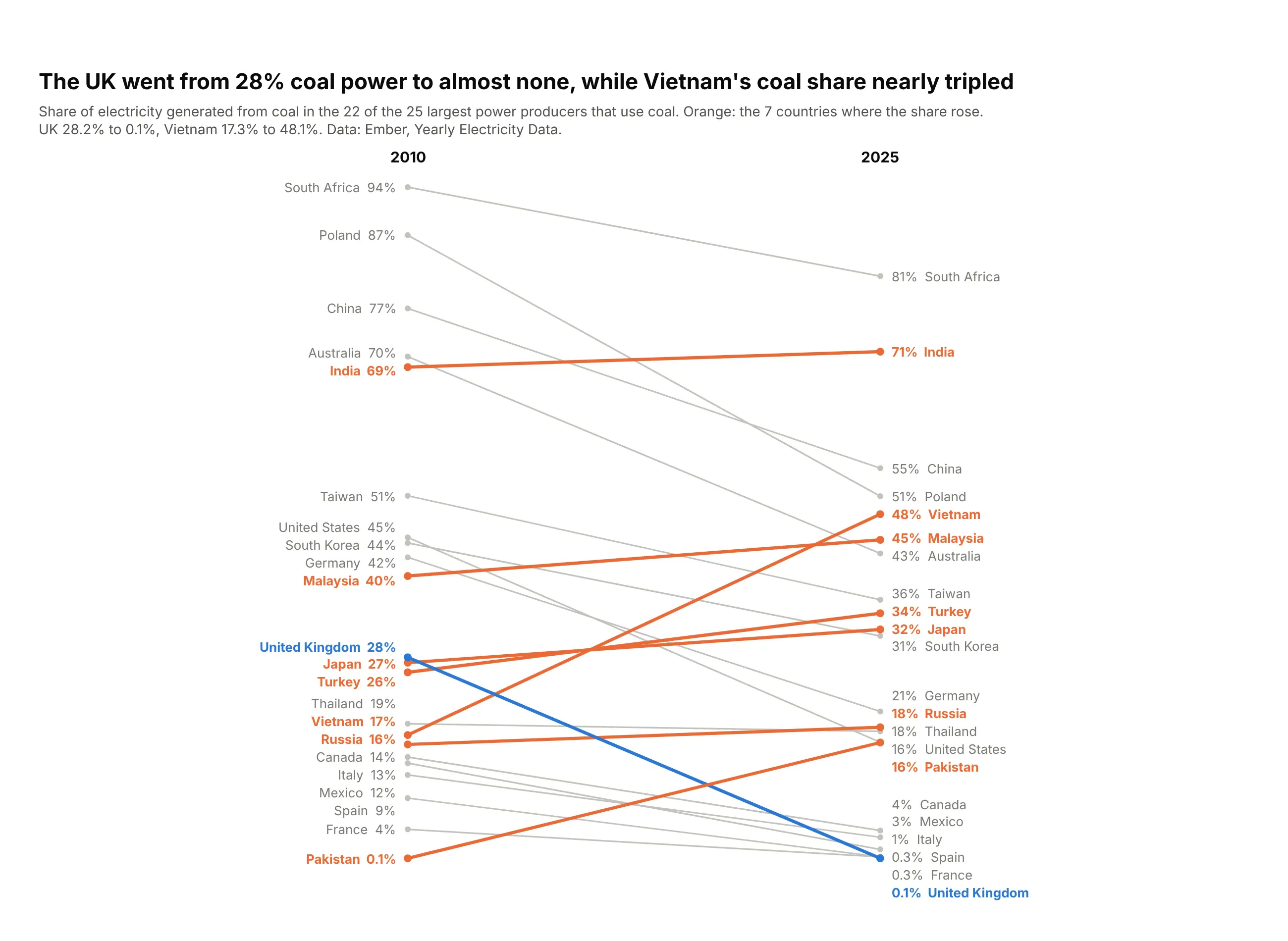
Slope charts look like this:

Slope chart of coal's share of electricity in 2010 and 2025 in 22 large power producers. The United Kingdom falls from 28% to 0.1% in blue; Vietnam rises from 17% to 48% and six other countries rise in orange, including Pakistan from 0.1% to 16%

Data: Ember, Yearly Electricity Data.

How do you read a slope chart? In the example above, notice these things:

Each line is one country, running from its share of electricity made from coal in 2010 on the left to its share in 2025 on the right. Both ends sit on the same vertical scale, so a higher point always means a larger share.
The angle of a line is the change, so the steepest lines are the biggest moves. The blue United Kingdom line ends with the lowest coal share on the chart, and Poland's gray line falls even further, by 36 points.
Orange marks the seven countries where the coal share rose, so they stand out against the gray ones that fell. Vietnam's line climbs the steepest and crosses ten other lines on its way up.
The labels at each end replace both the axis and the legend, and where two lines cross, those two countries swapped places. Pakistan starts at the very bottom and ends level with the United States.
A slope chart shows only the two end years, so anything that happened in between is hidden. India's almost flat line leaves out that its coal share went up to 77% in 2015 before falling back.

It's often used for charts like these:

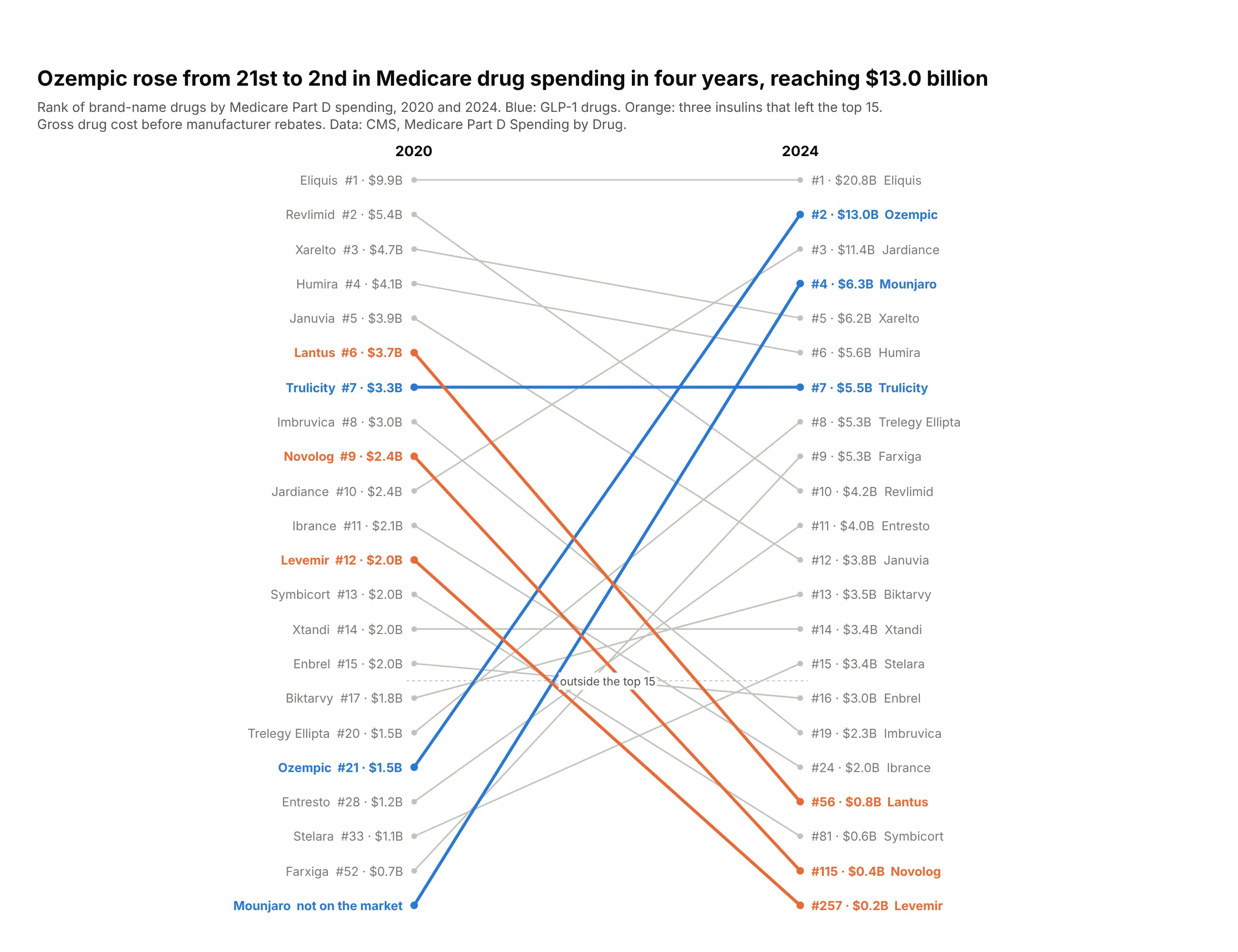
A ranking at two dates. Ozempic went from 21st to 2nd in Medicare Part D drug spending between 2020 and 2024, while three insulins fell out of the top 15. Data: CMS, Medicare Part D Spending by Drug.

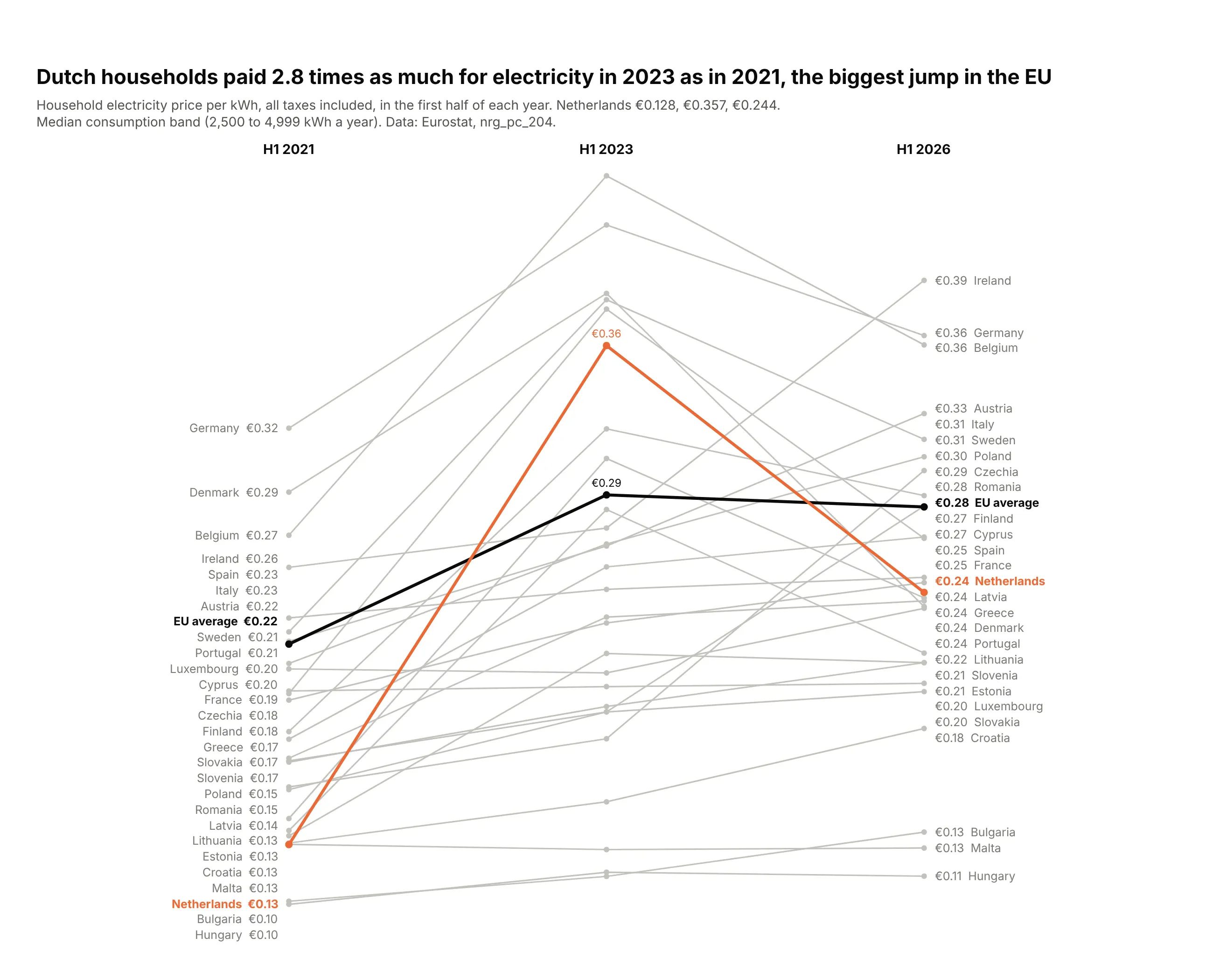
Three-column slope chart of household electricity prices per kWh in the first half of 2021, 2023 and 2026 in the 27 EU countries. The Netherlands in orange goes from €0.13 to €0.36 and back to €0.24; the EU average in black goes from €0.22 to €0.29 to €0.28

A shock and the recovery, with a third column. Dutch households paid €0.128 per kWh in early 2021, €0.357 in early 2023 and €0.244 in 2026, the largest jump in the EU. Data: Eurostat, nrg_pc_204.

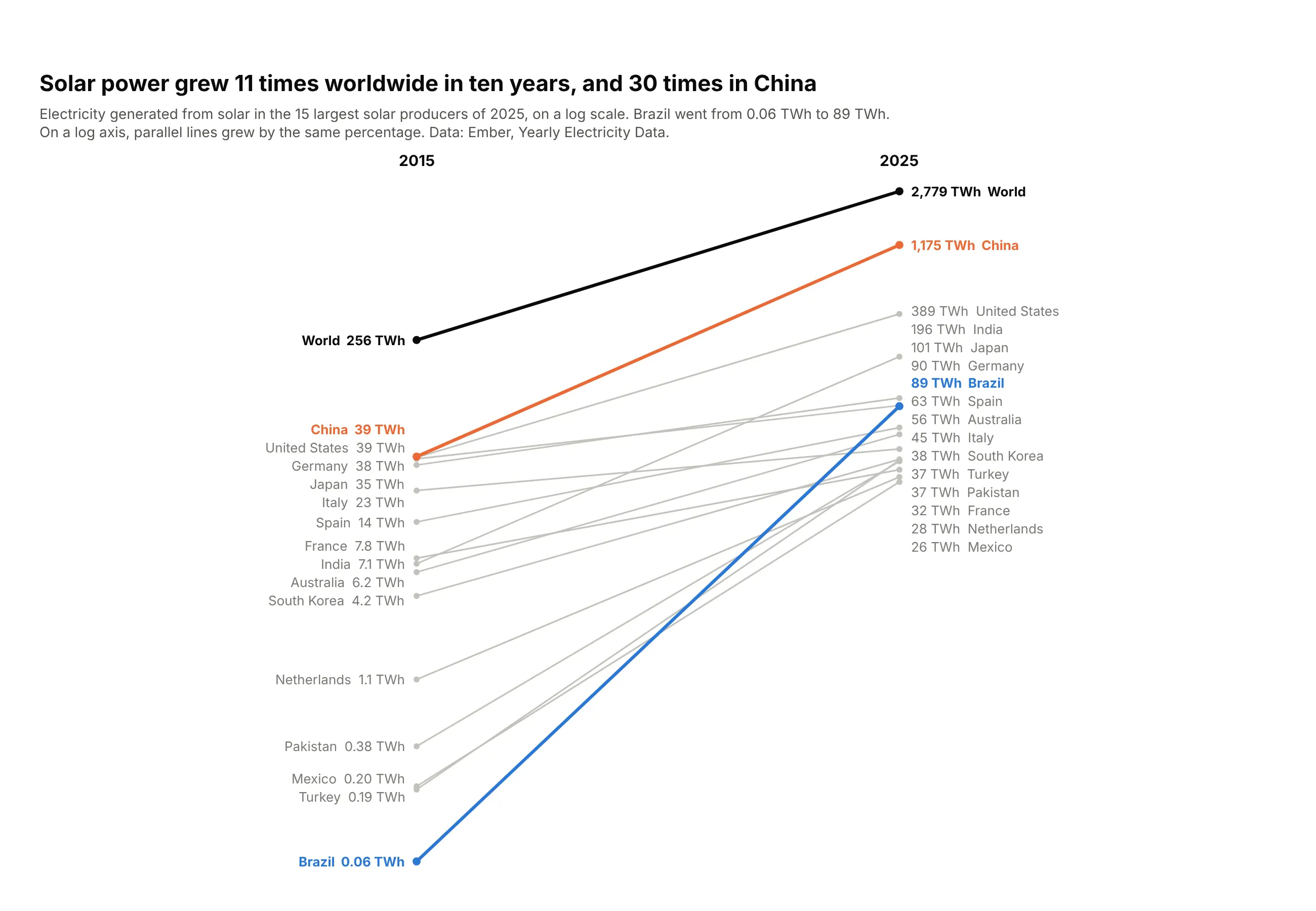
Slope chart on a log axis of solar generation in 2015 and 2025 for the 15 largest producers and the world. The world goes from 256 to 2,779 TWh in black, China from 39 to 1,175 TWh in orange, and Brazil from 0.06 to 89 TWh in blue

Growth on a log axis. World solar generation grew 11 times between 2015 and 2025 and China's 30 times, and on a log axis equal slopes mean equal growth rates. Data: Ember, Yearly Electricity Data.

A short history

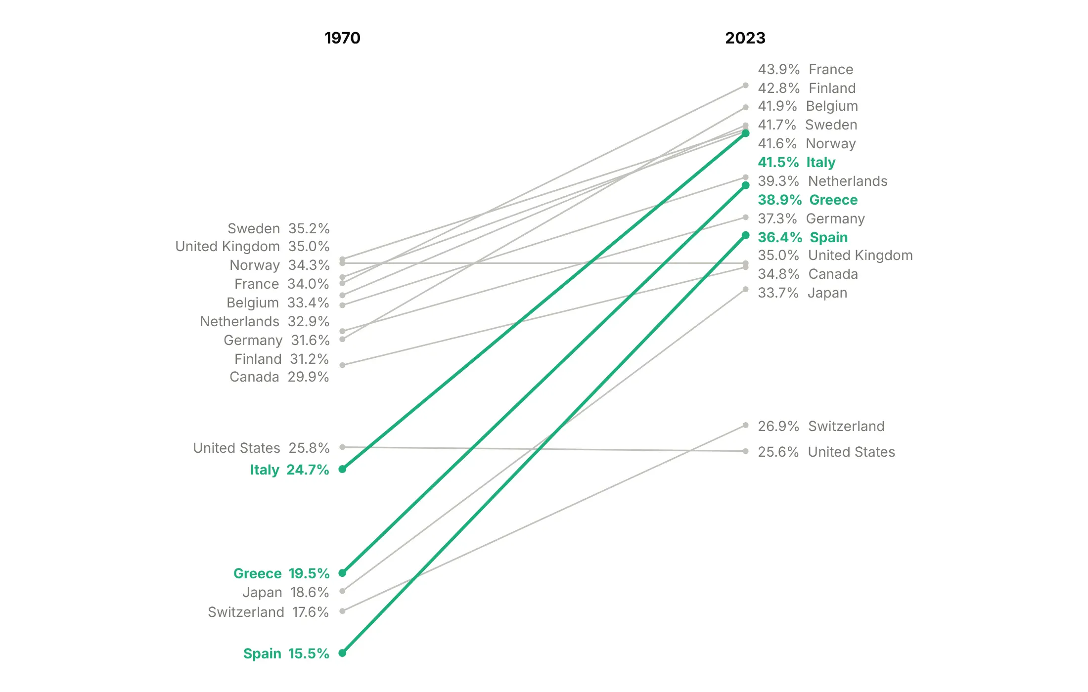
Edward Tufte published the first slope chart on page 158 of The Visual Display of Quantitative Information (Graphics Press, 1983). It compared current receipts of government as a share of GDP in 15 countries in 1970 and 1979, and he called it a table-graphic, because it reads as a table whose rows are joined by lines. Here it is redrawn with Plotly on the closest OECD series:

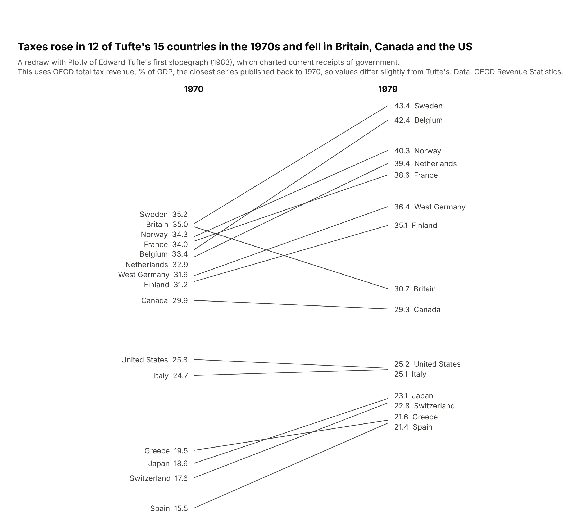
A redraw of Tufte's 1983 slopegraph: total tax revenue as a percentage of GDP in 1970 and 1979 for 15 countries, in thin dark lines with names and values at both ends. Sweden rises from 35.2 to 43.4 and Spain from 15.5 to 21.4, while Britain falls from 35.0 to 30.7 and Canada and the United States fall slightly

The form spread on the web after Charlie Park's 2011 essay Edward Tufte's "Slopegraphs", which also notes that Tufte named it a slopegraph on his forum that year. Example 1 under "More slope chart examples" redraws Tufte's chart with 2023 data.

Alternatives to a slope chart

Here's the same coal data for 8 countries drawn six ways. Some are better for the question, some worse, some just different:

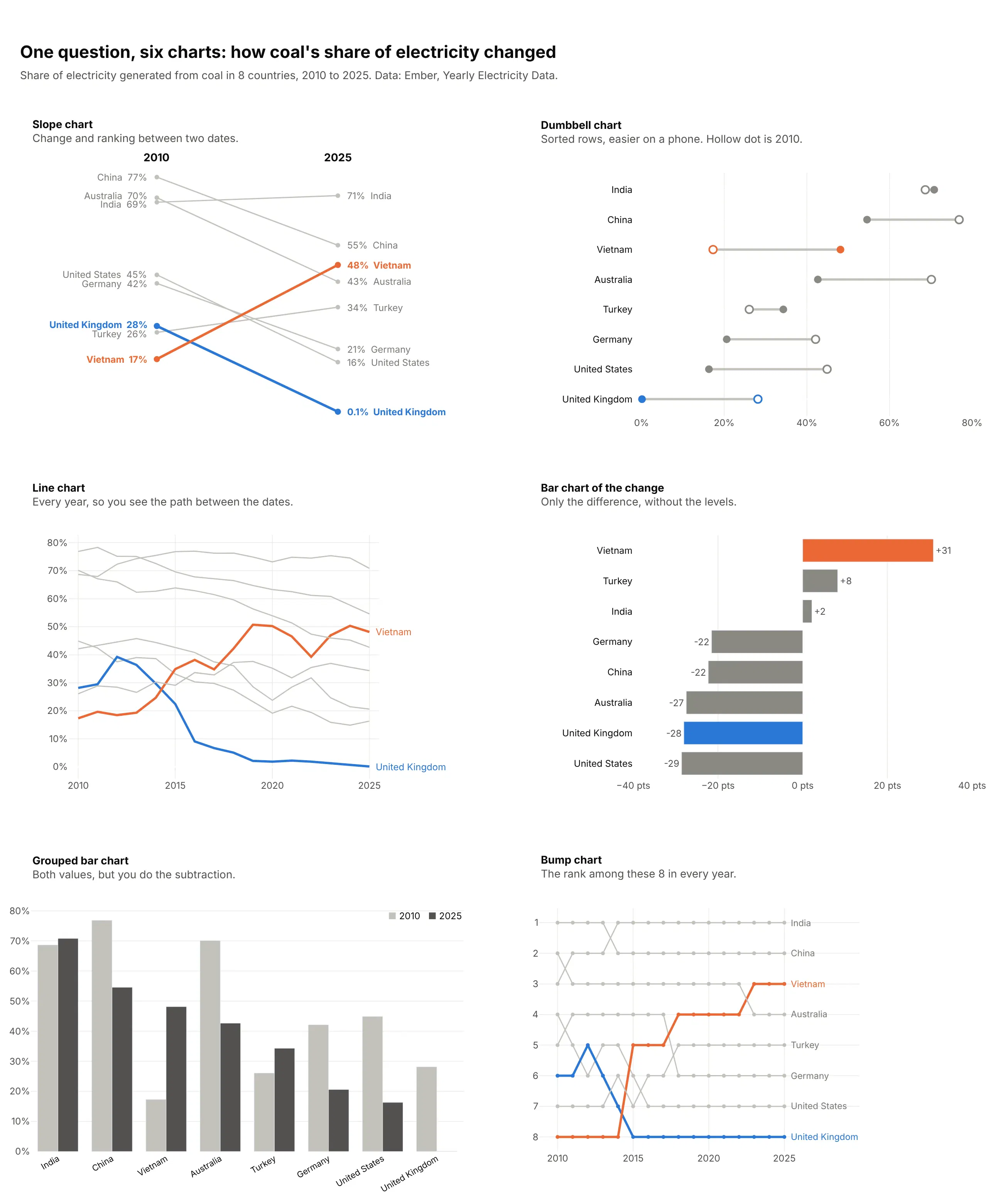
The same coal share data for 8 countries drawn six ways: a slope chart of 2010 and 2025, a dumbbell chart sorted by 2025, a line chart of every year from 2010 to 2025, a bar chart of the change (Vietnam +31 points, the UK -28, the US -29), a grouped bar chart of both years, and a bump chart of each country's rank among the 8 in every year

Dumbbell chart (works too, and better on a phone). Both values sit on one horizontal line per item, so you can sort the rows and fit more items, but crossings and rank changes are harder to see. See our dumbbell chart guide.
Line chart (better when the path matters). Two dates hide what happened between them. Vietnam's coal share reached 51% in 2019, dipped to 39% in 2022 and came back, which only the line chart shows.
Bar chart of the change (better when only the change matters). It ranks the changes from Vietnam's +31 points to the US's -29, but drops the starting levels. Bars on a shared baseline are also the most precise way to compare numbers, as Cleveland and McGill (1984) measured.
Grouped bar chart (worse). It shows both values but makes the reader do the subtraction for every country, and the ranking at each date is hard to follow.
Bump chart (different). A slope chart of ranks over many periods. It shows every reshuffle, but not how far apart the values are. See our bump chart guide.

How to make a slope chart

With AI

ChatGPT, Claude Code, GitHub Copilot, Cursor and other AI tools are excellent at writing Plotly code. Name Plotly in the prompt, say which columns are the dates and which lines to highlight, and list the checks you want:

Make a plotly slope chart from prices.csv (columns: country, price_2021, price_2023, price_2026).

- One go.Scatter line per country between x positions 0, 1 and 2; hide both axes.
- Name and value as annotations at both ends ("Netherlands €0.13" / "€0.24 Netherlands").
  Nudge labels apart so no two are closer than 18 px, keeping their order.
- Netherlands in #eb6834 and the EU average in #0b0b0b, 3 px; every other line #c3c2bc, 1.5 px.
- Print the middle value above the marker for the highlighted lines only.
- Inter font, white background, a title that states the main takeaway, the source in a subtitle.
- Check that every country has all three values and print any that don't.

With Plotly Studio

Plotly Studio is a desktop app where you point an AI at a dataset and it builds charts and a Dash app around your questions. Ask for a slope chart and say what to highlight:

Show a slope chart of coal's share of electricity by country in 2010 and 2025. Label each country's name and value at both ends, color the countries where the share rose in orange and the UK in blue, and gray the rest. Add a dropdown to pick the two years.

Make a slope chart in Python or JavaScript

This is the code AI tools write under the hood. In Python, this helper makes a slope chart with Plotly by drawing one go.Scatter per row of a DataFrame, writing the labels as annotations and nudging labels that would overlap apart. Every example in this guide builds on a longer version of it:

import numpy as np
import pandas as pd
import plotly.graph_objects as go


def spread(y, gap):
    """Push positions apart until neighbors are at least `gap` apart, keeping their order."""
    order = np.argsort(y)
    p = np.asarray(y, dtype=float)[order]
    for _ in range(500):
        overlap = gap - np.diff(p)
        if overlap.max(initial=0) <= 1e-9:
            break
        for k in np.flatnonzero(overlap > 0):
            p[k] -= overlap[k] / 2
            p[k + 1] += overlap[k] / 2
    out = np.empty_like(p)
    out[order] = p
    return out


def make_slope(df, label, start, end, highlight=None, fmt="{:,.0f}", height=800, gap_px=18):
    """Slope chart of df[start] -> df[end], one line per row; `highlight` maps labels to colors."""
    highlight = highlight or {}
    fig = go.Figure()
    for _, r in df.sort_values(label, key=lambda s: s.isin(list(highlight))).iterrows():
        hl = r[label] in highlight
        fig.add_scatter(x=[0, 1], y=[r[start], r[end]], mode="lines+markers", name=r[label],
                        line=dict(color=highlight.get(r[label], "#c3c2bc"), width=3 if hl else 1.5),
                        showlegend=False)
    lo, hi = df[[start, end]].min().min(), df[[start, end]].max().max()
    gap = gap_px * (hi - lo) / (height - 200)  # pixels -> data units
    for x, col in [(0, start), (1, end)]:
        for (_, r), y in zip(df.iterrows(), spread(df[col], gap)):
            value = fmt.format(r[col])
            fig.add_annotation(x=x, y=y, showarrow=False, xanchor="right" if x == 0 else "left",
                               xshift=-10 if x == 0 else 10,
                               text=f"{r[label]}  {value}" if x == 0 else f"{value}  {r[label]}",
                               font_color=highlight.get(r[label], "#7a7974"))
        fig.add_annotation(x=x, y=1.02, yref="paper", text=f"<b>{col}</b>", showarrow=False)
    fig.update_xaxes(visible=False, range=[-0.02, 1.02], domain=[0.3, 0.7])
    fig.update_yaxes(visible=False)
    fig.update_layout(height=height, plot_bgcolor="white", margin=dict(t=120, b=40))
    return fig


tax = pd.DataFrame({
    "country": ["Spain", "France", "United Kingdom", "Japan", "United States"],
    "1970": [15.5, 34.0, 35.0, 18.6, 25.8],
    "2023": [36.4, 43.9, 35.0, 33.7, 25.6],
})
make_slope(tax, "country", "1970", "2023", fmt="{:.1f}%",
           highlight={"Spain": "#eb6834", "United States": "#2a78d6"}).show()

In JavaScript, plotly.js builds the same chart from one scatter trace per line and an annotation for each label:

<div id="chart"></div>
<script src="https://cdn.plot.ly/plotly-4.1.1.min.js"></script>
<script>
  const tax = {"Spain": [15.5, 36.4], "France": [34.0, 43.9], "United Kingdom": [35.0, 35.0],
               "Japan": [18.6, 33.7], "United States": [25.8, 25.6]};
  const color = {"Spain": "#eb6834", "United States": "#2a78d6"};
  const traces = [], annotations = [];
  for (const [country, [a, b]] of Object.entries(tax)) {
    const c = color[country] || "#c3c2bc";
    traces.push({x: [0, 1], y: [a, b], mode: "lines+markers", line: {color: c, width: color[country] ? 3 : 1.5},
                 name: country, showlegend: false});
    annotations.push({x: 0, y: a, text: `${country}  ${a.toFixed(1)}%`, xanchor: "right", xshift: -10, showarrow: false},
                     {x: 1, y: b, text: `${b.toFixed(1)}%  ${country}`, xanchor: "left", xshift: 10, showarrow: false});
  }
  Plotly.newPlot("chart", traces, {
    annotations: annotations,
    xaxis: {visible: false, range: [-0.02, 1.02], domain: [0.3, 0.7]},
    yaxis: {visible: false},
    plot_bgcolor: "white"
  });
</script>

The JavaScript version has no label nudging, so France and the United Kingdom, 34.0% and 35.0% in 1970, print on top of each other. Use the spread function from the Python version, or make the chart taller, when labels collide.

Share it

Every Plotly chart has a Share chart button (the cloud icon in its toolbar) that uploads it to Plotly Cloud and gives you a link. Only you can see it until you change its visibility.

For a live app, put the chart in a Dash app and publish it with the Plotly Cloud CLI. Coding agents can run these commands for you:

pip install "dash[cloud]"
plotly user login
plotly app publish

If your data has to stay in your own cloud or data center, publish to Dash Enterprise instead.

Dos and don'ts

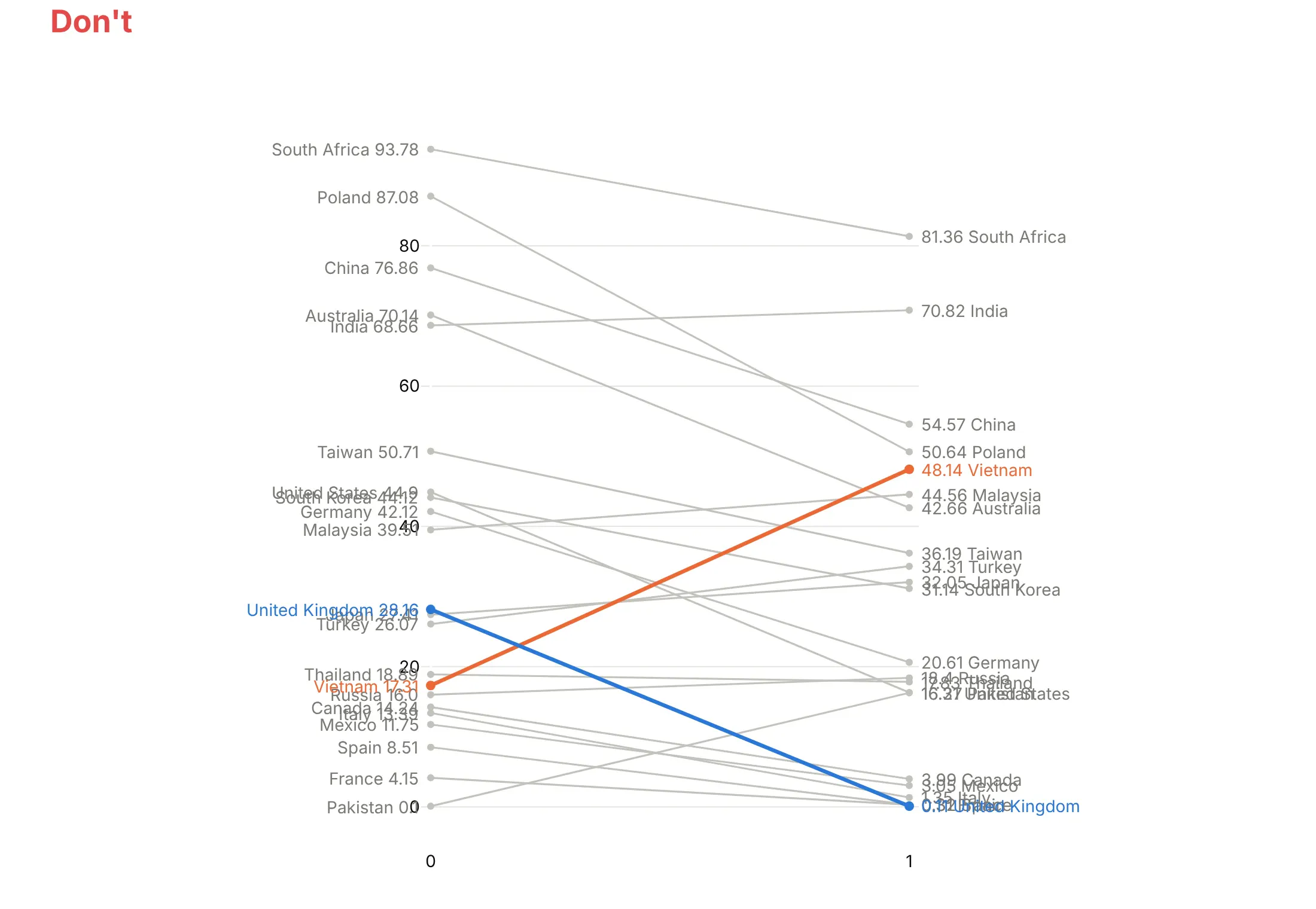
A slope chart is mostly labels, so most of the mistakes are about labels. Here is the coal data both ways, with the same colors in both charts.

Don't print labels at their exact positions, where close values land on top of each other, show raw values like 28.16 and 0.11, leave the x axis as 0 and 1 instead of the years, or keep a y axis and gridlines that the labels already replace:

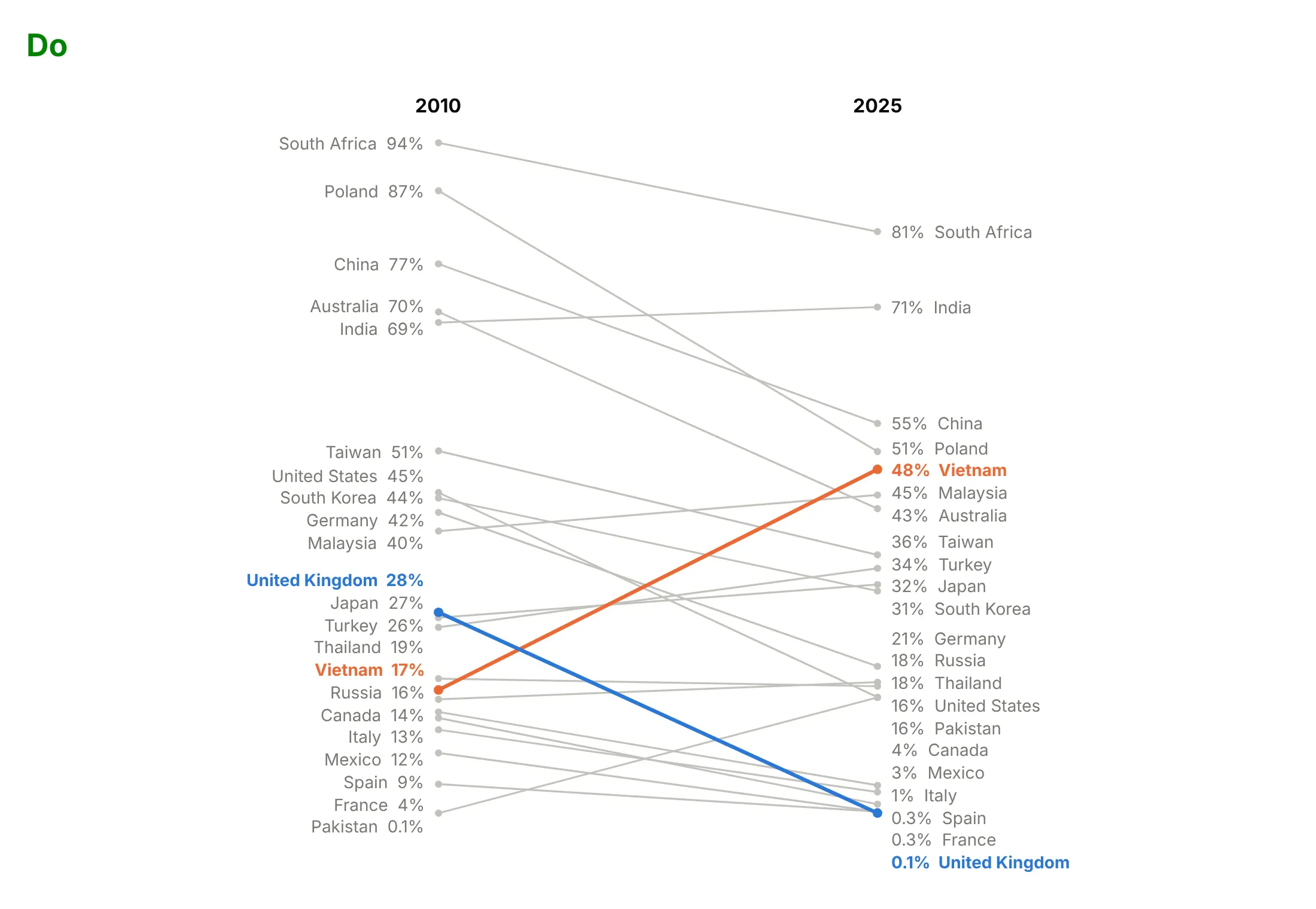
The coal share data for 22 countries as a slope chart with the United Kingdom in blue and Vietnam in orange, but with labels such as 16.31 United States and 16.27 Pakistan printed on top of each other, raw two-decimal values, x ticks 0 and 1 instead of 2010 and 2025, and a y axis with gridlines whose tick numbers collide with the labels

Do nudge labels apart so each one is readable, round the values, put the years above the columns and drop the axes:

The same coal data as a styled slope chart with names and rounded values at both ends nudged apart, 2010 and 2025 above the columns, the United Kingdom in blue falling from 28% to 0.1%, Vietnam in orange rising from 17% to 48%, and every other country in gray

Use color for one thing

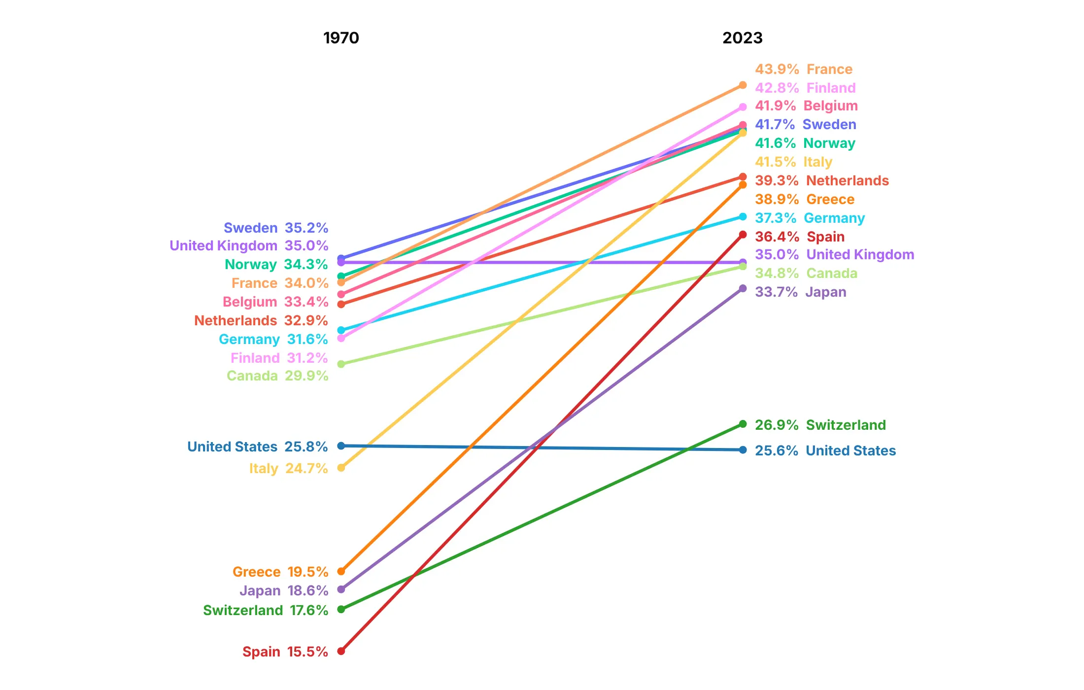
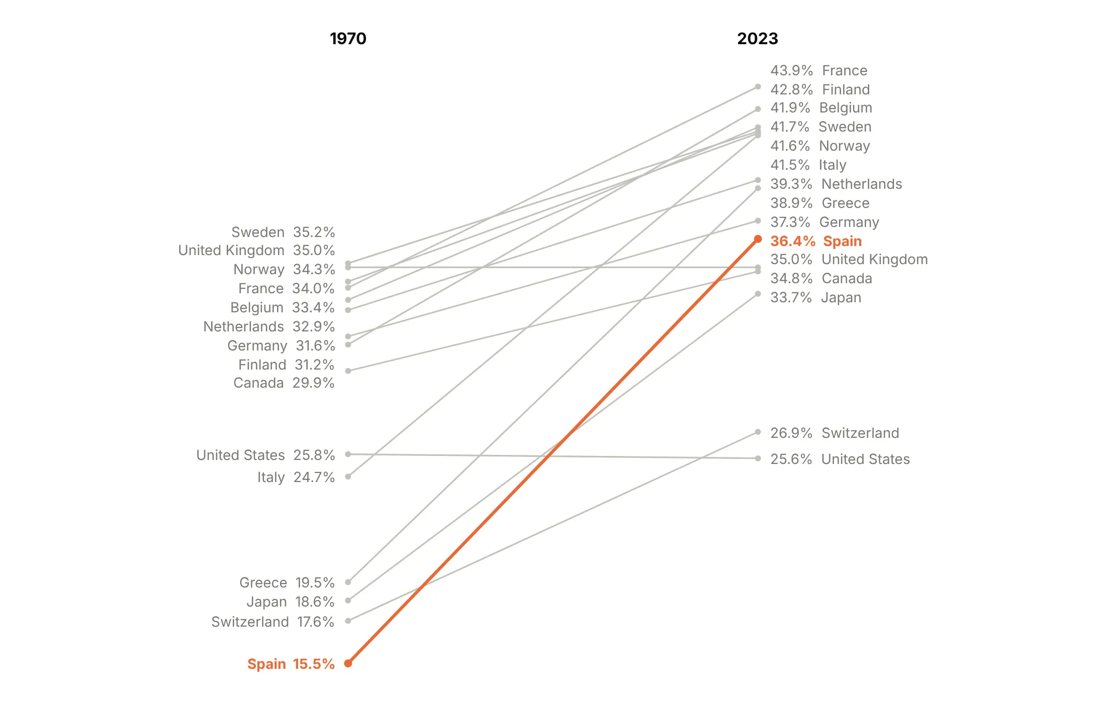
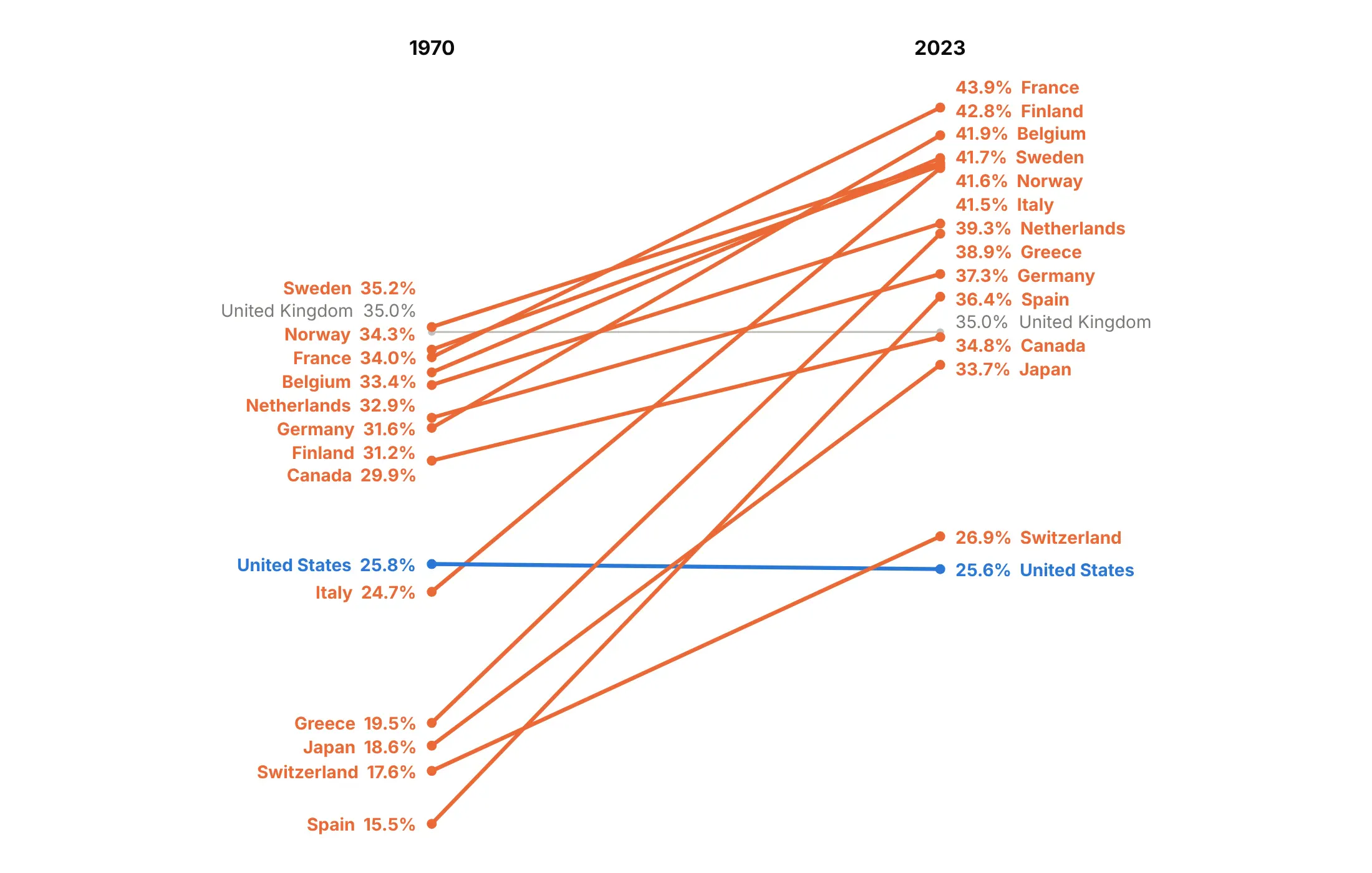
A color per line makes readers look for a meaning that isn't there. Here are four options on Tufte's 15 countries with 2023 data.

A color for every line (avoid). Fifteen colors, and none of them means anything.

Slope chart of tax revenue as a share of GDP in 1970 and 2023 for 15 countries, with a different color for every line

One story in color. Spain's rise from 15.5% to 36.4% of GDP was the largest, so it's the only colored line.

The same tax revenue slope chart with Spain in orange and every other country in gray

Color by direction. Works when lines go both ways. Here 13 of the 15 countries rose (orange), so the one that fell, the United States, stands out in blue, and the United Kingdom, unchanged at 35.0%, stays gray.

The same tax revenue slope chart with 13 rising countries in orange, the United States in blue and the United Kingdom in gray

Highlight a group. Spain, Italy and Greece all collected less than 25% of GDP in tax in 1970 and between 36% and 42% in 2023.

The same tax revenue slope chart with Spain, Italy and Greece in green and the other 12 countries in gray

Use a log axis for growth

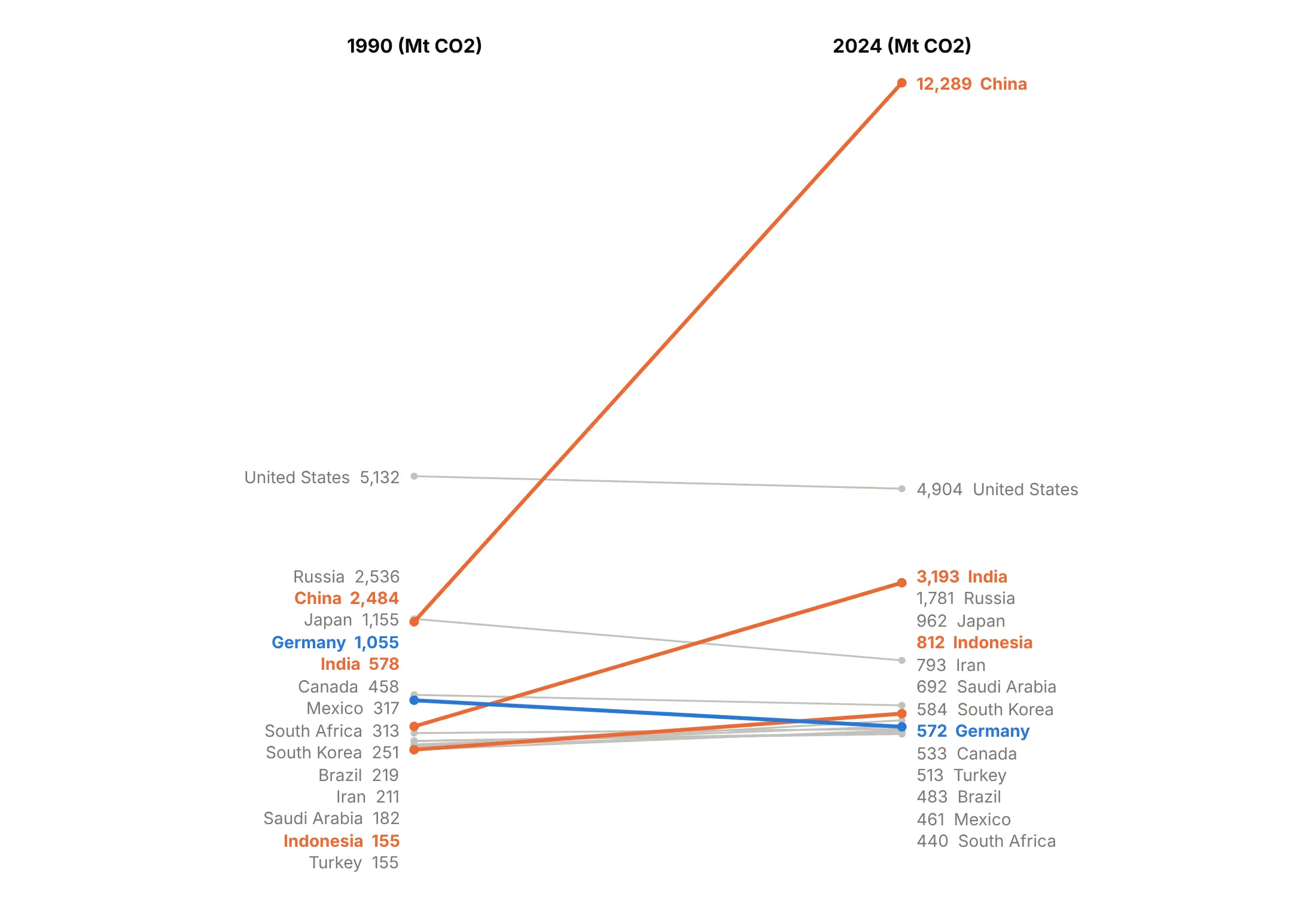
On a linear axis the slope is the absolute change, so the biggest items dominate. Here China's line takes the whole height and the other 14 countries pile up at the bottom:

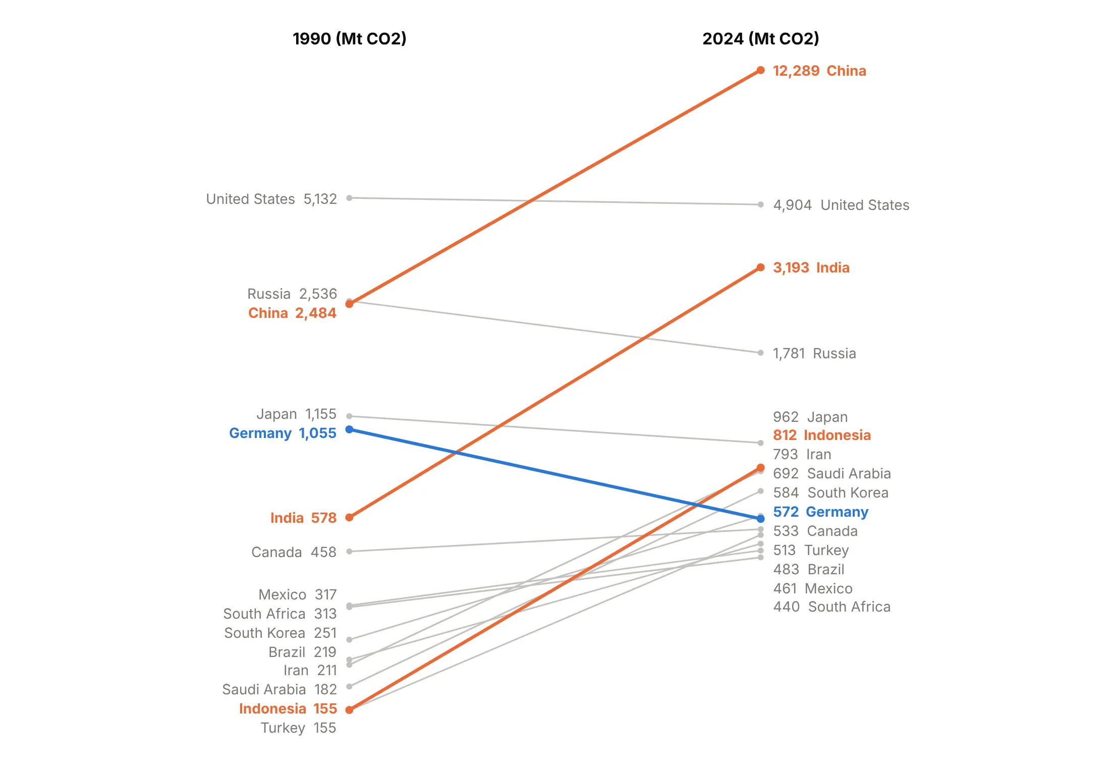
Fossil CO2 emissions in million tonnes in 1990 and 2024 for the 15 largest emitters on a linear axis. China in orange rises from 2,484 to 12,289 and dominates the chart, while most other labels are pushed together at the bottom

On a log axis the slope is the percentage change, so Indonesia's growth from 155 to 812 million tonnes (5.2 times) looks as steep as China's (4.9 times) and India's (5.5 times):

The same CO2 data on a log axis, where India (578 to 3,193), Indonesia (155 to 812) and China (2,484 to 12,289) in orange have similar slopes, and Germany in blue falls from 1,055 to 572

Choose values or ranks

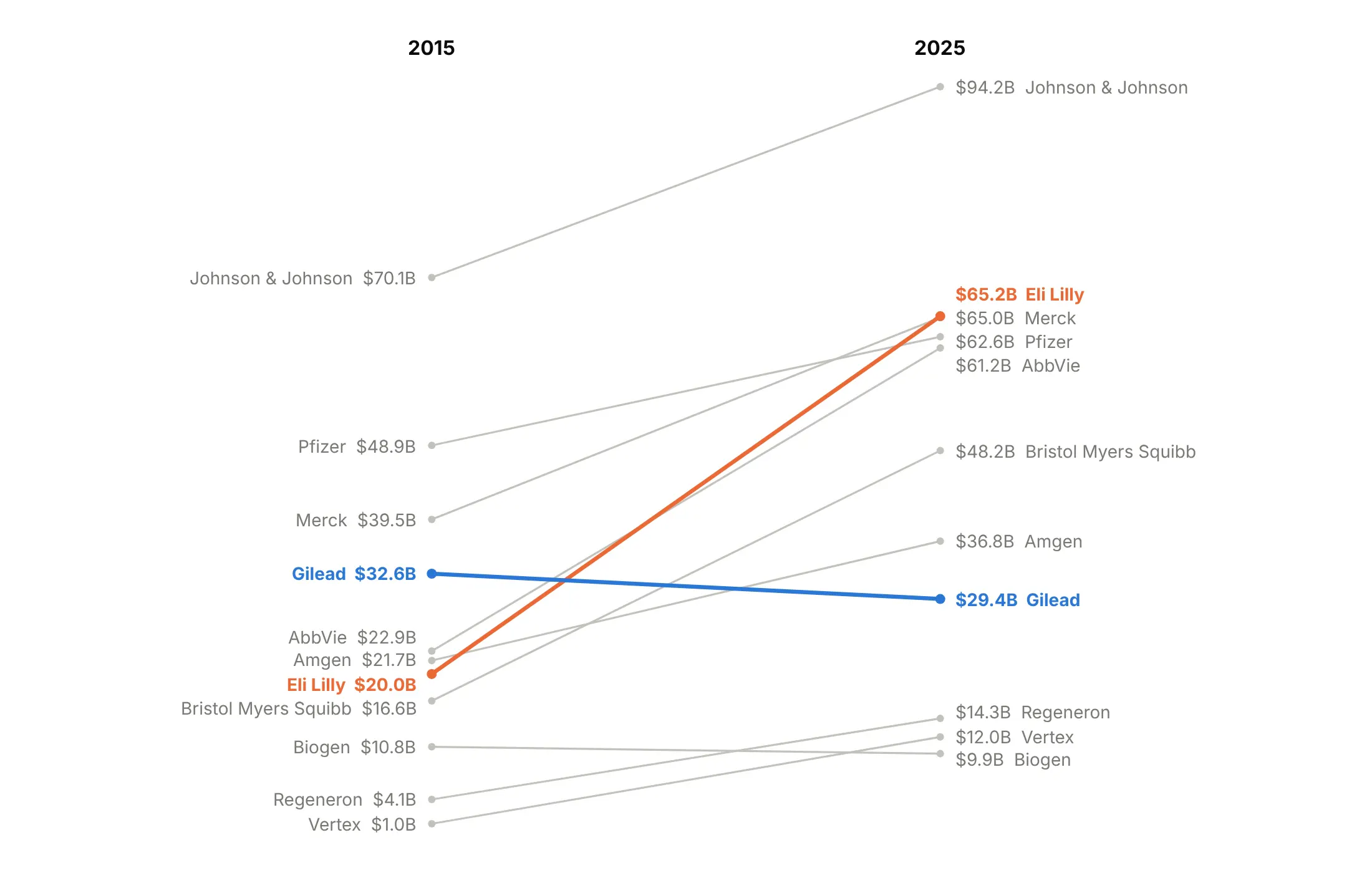
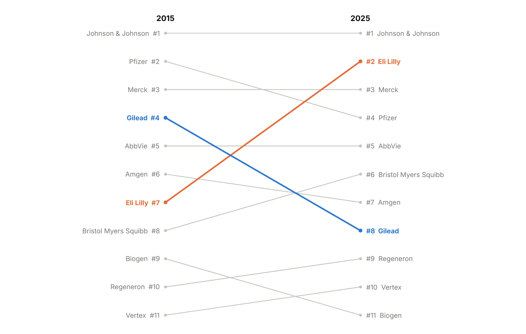
A value slope chart shows how far apart items are. Eli Lilly's revenue went from $20.0 billion to $65.2 billion, and in 2025 Lilly, Merck, Pfizer and AbbVie are within $4.0 billion of each other:

The revenue of 11 drug makers in 2015 and 2025 as a value slope chart. Eli Lilly in orange rises from $20.0B to $65.2B, Gilead in blue falls from $32.6B to $29.4B, and Johnson & Johnson is highest at $94.2B

A rank slope chart spaces items evenly, which makes the reshuffle clear but hides those gaps. Lilly rises from 7th to 2nd and Gilead falls from 4th to 8th:

The same 11 drug makers as a rank slope chart with rank 1 at the top. Eli Lilly in orange goes from #7 to #2 and Gilead in blue from #4 to #8

Checklist

Write a title that states the takeaway with the two numbers: "Ozempic rose from 21st to 2nd in Medicare drug spending".
Label both ends directly with name and value, rounded to the precision the story needs.
Name the columns (the years) above the lines.
Gray everything except one to three stories, and draw the highlights thicker.
Nudge labels apart so close values stay readable.
Use a log axis when values span orders of magnitude or the story is growth rates.
Add a zero line when values cross zero (example 6).

Don't

Use a legend or a y axis, because the labels at the ends do the job.
Leave close labels overlapping.
Give every line its own color.
Connect more than three columns. Use a line chart or a bump chart instead.
Compare different units on a linear axis.

Options to customize

These are the go.Scatter and layout options that build a slope chart. The full reference is in the Plotly scatter documentation and the text and annotations page.

go.Scatter(x=[0, 1], y=[a, b]): one line per item between two x positions; use 0, 1, 2 for three columns.
mode="lines+markers": draws the line and the end dots; add +text to print middle values.
line.color, line.width: gray context lines and thicker highlights.
text, textposition: text on the points, for middle values in three-column charts.
cliponaxis=False: lets text and markers draw outside the plot area, for labels at the top or bottom edge.
hovertemplate, customdata: the column name and value on hover.
layout.annotations (x, y, xanchor, xshift, showarrow=False): the direct labels at each end.
xaxis.visible=False, xaxis.range, xaxis.domain: hides the x axis, and the domain leaves room for the labels.
yaxis.visible=False: hides the y axis once the values are labeled.
yaxis.type="log": a log scale for growth rates or orders of magnitude; annotation y is then the log10 value.
yaxis.range=[max, min]: reverses the axis, for rank charts with 1 at the top.
layout.shapes: zero lines and dotted "outside the top N" dividers.
xaxis2, yaxis2, domain: several slope charts side by side in one figure.

More slope chart examples

Ten more slope charts built from real public data, each with its source, the technique that makes it work and a prompt to rebuild it.

1. Tufte's slopegraph with 2023 data

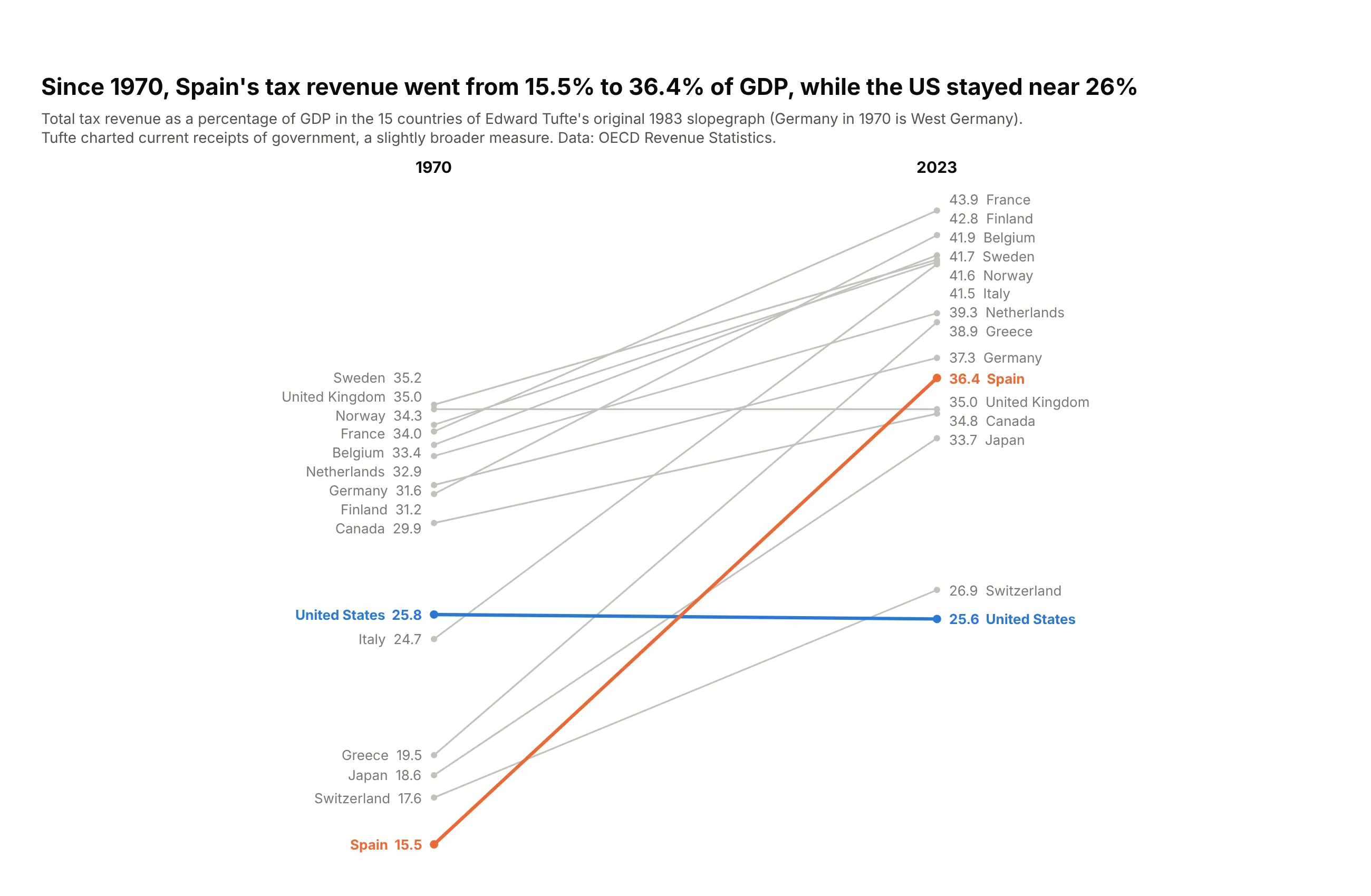
Slope chart of tax revenue as a share of GDP in 1970 and 2023 in the 15 countries of Tufte's original slopegraph. Spain rises from 15.5% to 36.4% in orange; the United States goes from 25.8% to 25.6% in blue

Tufte's 15 countries, 53 years later. Spain's tax revenue went from 15.5% to 36.4% of GDP, the largest rise, while the US went from 25.8% to 25.6%. Data: OECD Revenue Statistics.

Tip: names and values on both sides, as in Tufte's original, so it reads as a table and a chart.

Get the data from OECD Revenue Statistics, total tax revenue as a percentage of GDP
(columns: country, pct_1970, pct_2023; the 15 countries of Tufte's 1983 slopegraph).

Build a Tufte-style plotly slope chart, 1970 to 2023.
- Names and values at both ends, one decimal, no axes or gridlines.
- Spain #eb6834, United States #2a78d6, the rest #c3c2bc. Note that Germany in 1970 is West Germany.

2. European gas cost 8.4 times its 2019 price

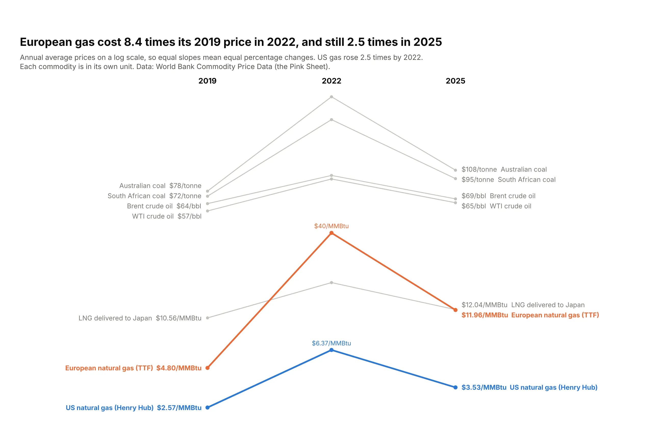
Three-column slope chart of energy commodity prices in 2019, 2022 and 2025 on a log axis. European gas rises from $4.80 to $40 per MMBtu and falls to $11.96 in orange; US gas goes from $2.57 to $6.37 to $3.53 in blue; oil and coal lines in gray

European gas averaged $4.80 per MMBtu in 2019, $40.34 in 2022 and $11.96 in 2025, still 2.5 times the 2019 price. US gas peaked at 2.5 times its 2019 price. Data: World Bank Commodity Price Data (the Pink Sheet).

Tip: on a log axis slopes are percentage changes, so commodities in different units can share the chart.

Get the data from the World Bank's Commodity Price Data (the Pink Sheet), annual nominal prices
(columns: commodity, unit, price_2019, price_2022, price_2025; Brent, WTI, Australian and South African coal,
US gas, European gas, LNG Japan).

Build a three-column plotly slope chart on a log y axis.
- Labels carry the unit ("$40/MMBtu", "$78/tonne"), names at both ends.
- European gas #eb6834, US gas #2a78d6, the rest #c3c2bc. Title with Europe's 2022 and 2025 multiples.
- Escape "$" in labels (plotly treats $...$ as LaTeX).

3. Central banks cut after 2023, Japan finally raised

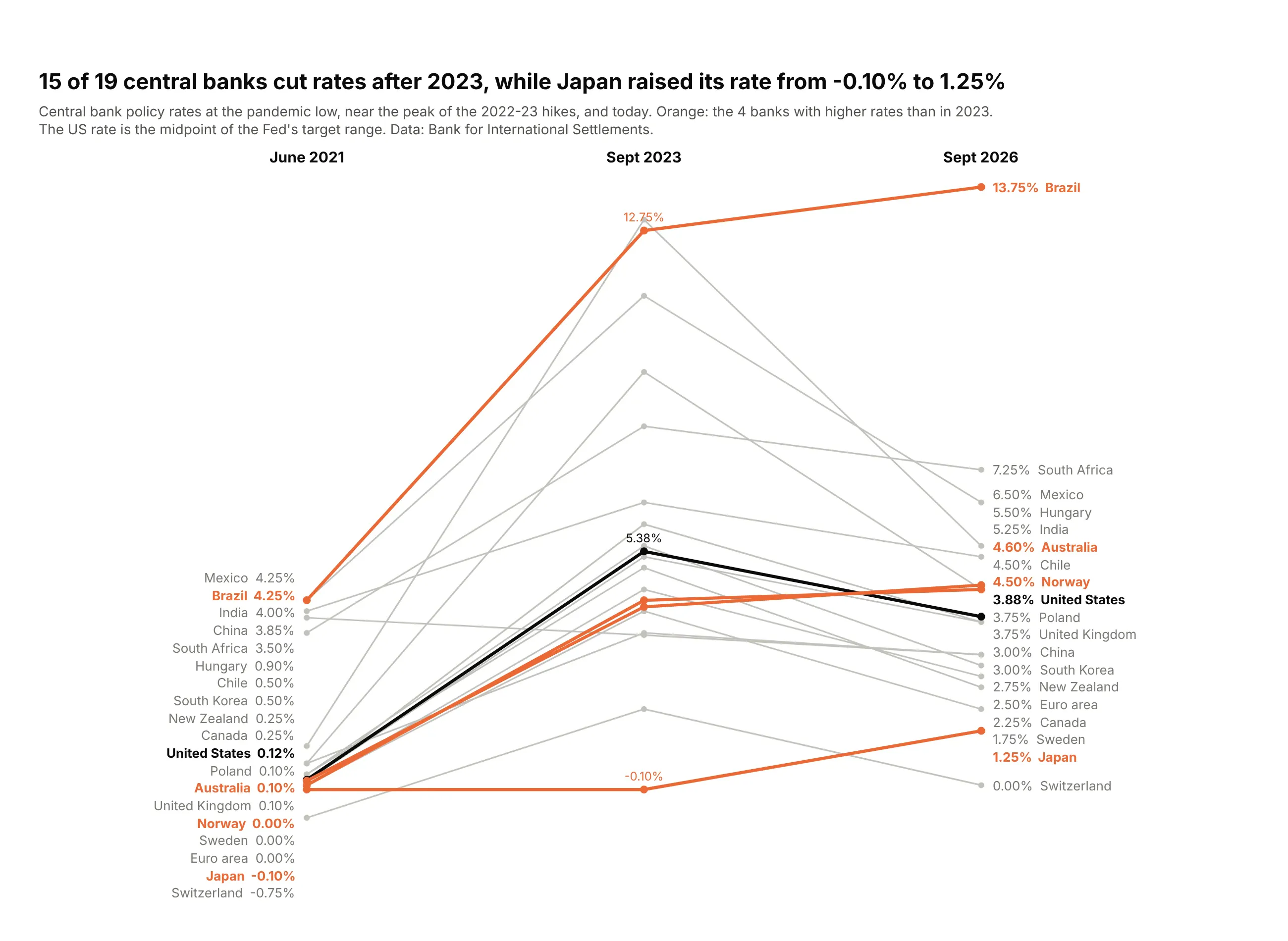
Three-column slope chart of policy rates in June 2021, September 2023 and September 2026 in 19 economies. Most lines rise and fall back; Japan (from -0.10% to 1.25%), Australia, Norway and Brazil are orange because their rates are higher than in 2023; the US is black at 0.12%, 5.38% and 3.88%

15 of 19 central banks had lower rates in September 2026 than in 2023. Japan went from -0.10% to 1.25%, and only China is below its 2021 level. Data: Bank for International Settlements.

Tip: three columns show the whole cycle, and coloring the lines that break the pattern finds the outliers.

Get the data from the BIS central bank policy rates dataset (WS_CBPOL), monthly
(columns: country, rate_2021_06, rate_2023_09, rate_2026_09; percent).

Build a three-column plotly slope chart for 19 large economies (leave out Argentina, Russia, Turkey).
- Lines whose 2026 rate is above 2023 in #eb6834, US in #0b0b0b, the rest #c3c2bc.
- Middle values only for Japan, Brazil and the US. Title with the count of cutters.

4. China's debt went from 29% to 99% of GDP

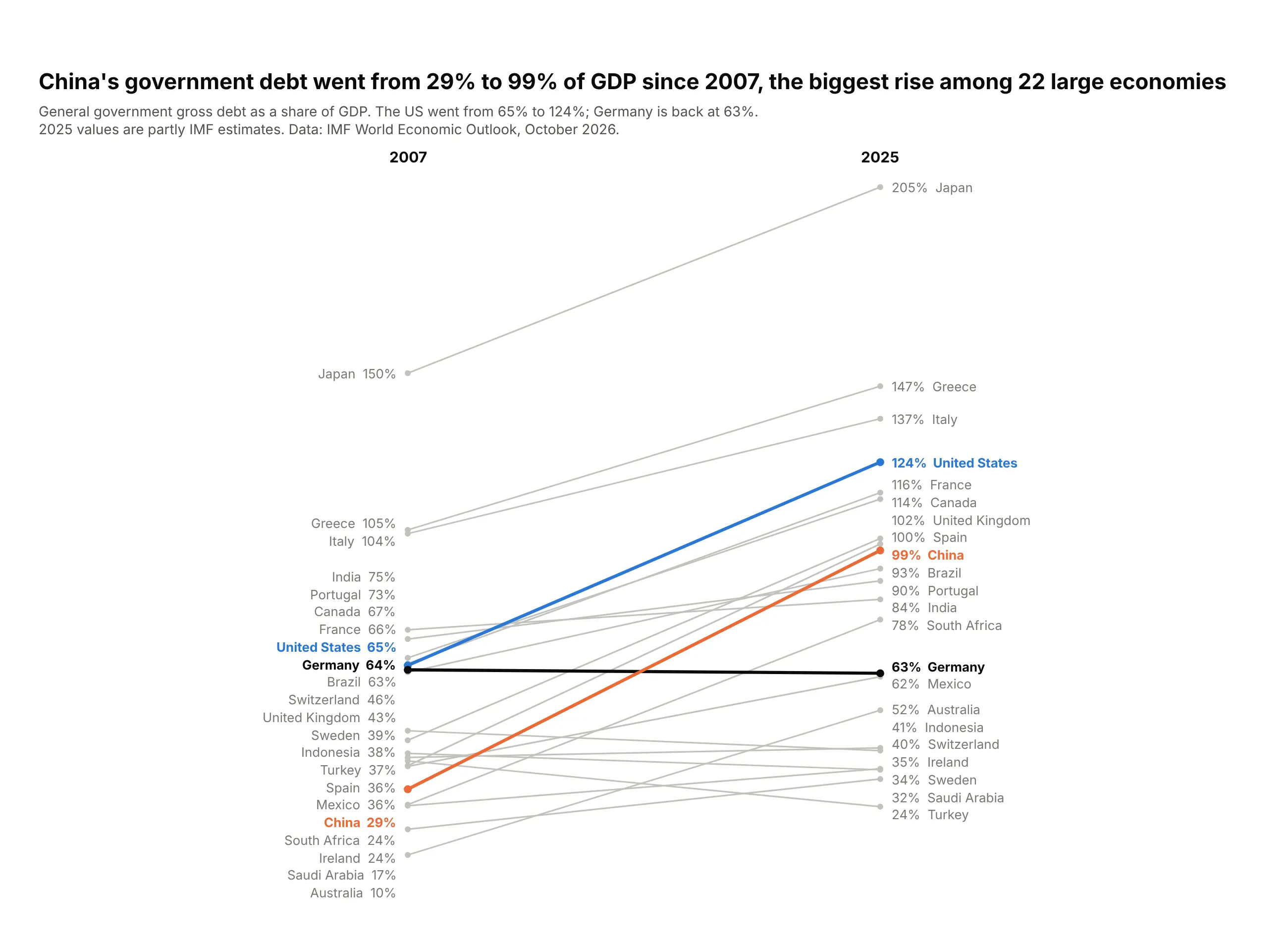
Slope chart of government debt as a share of GDP in 2007 and 2025 in 22 economies. China rises from 29% to 99% in orange, the US from 65% to 124% in blue, and Germany stays at 63% in black; Japan is highest at 205%

China's government debt rose from 29% of GDP in 2007 to 99% in 2025, the biggest rise of these 22 economies. The US went from 65% to 124%, and Germany ended where it started. Data: IMF World Economic Outlook, October 2026.

Tip: a flat line in a contrasting color (Germany) is a useful reference for the rising ones.

Get the data from the IMF World Economic Outlook (October 2026), general government gross debt, % of GDP
(columns: country, debt_2007, debt_2025).

Build a plotly slope chart, 2007 to 2025, for 22 large economies.
- China #eb6834, United States #2a78d6, Germany #0b0b0b, the rest #c3c2bc.
- Assert China has the largest rise. Note that 2025 values are partly estimates.

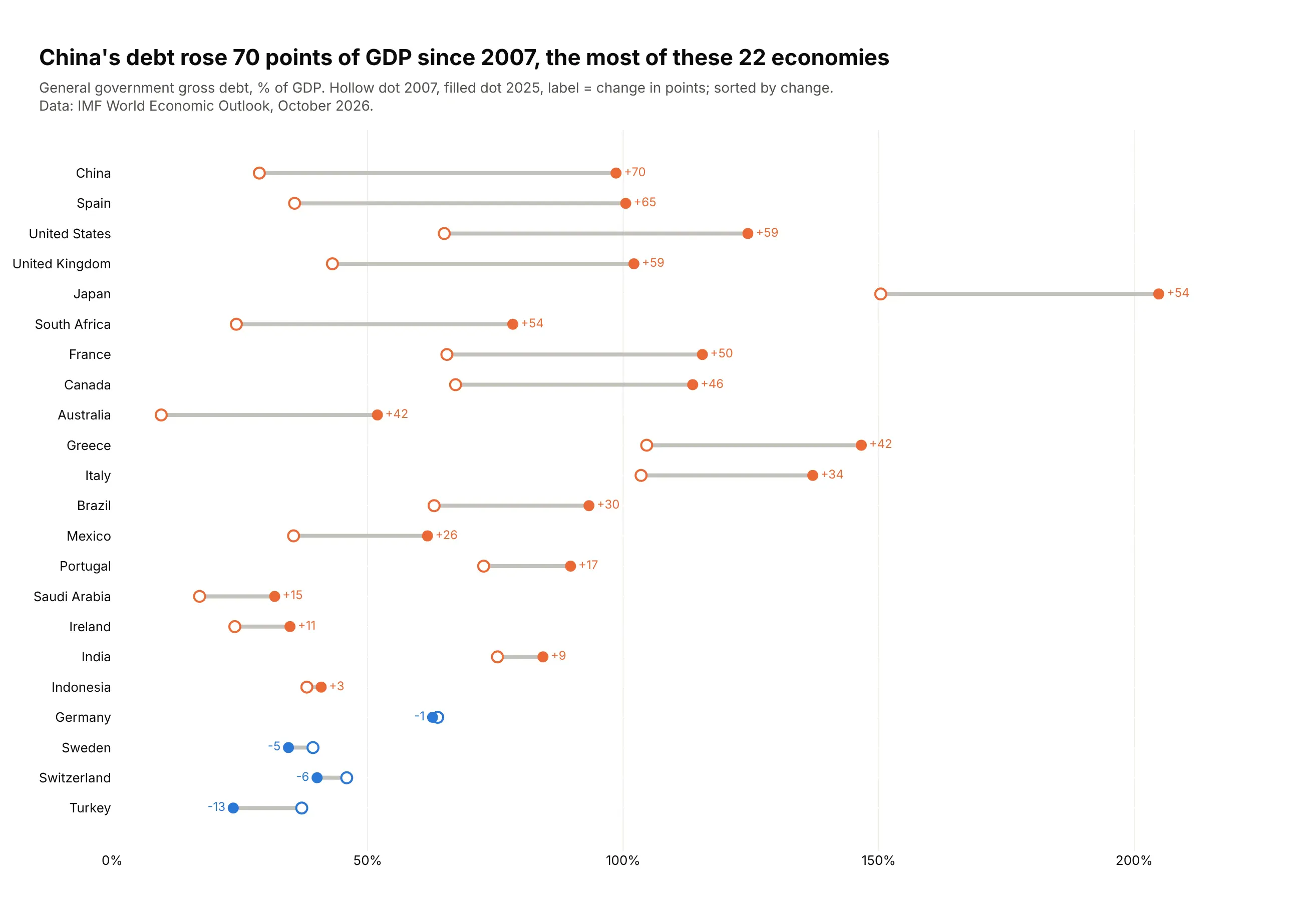
Another way to see it: a dumbbell chart sorted by the change shows the ranking of rises directly, with Germany, Sweden, Switzerland and Turkey the only four that fell.

Dumbbell chart of government debt in 2007 and 2025, sorted by change. China +70 points at the top, then Spain +65, the US and UK +59; Germany -1, Sweden -5, Switzerland -6 and Turkey -13 at the bottom in blue

5. Goldman Sachs Bank climbed from 18th to 7th

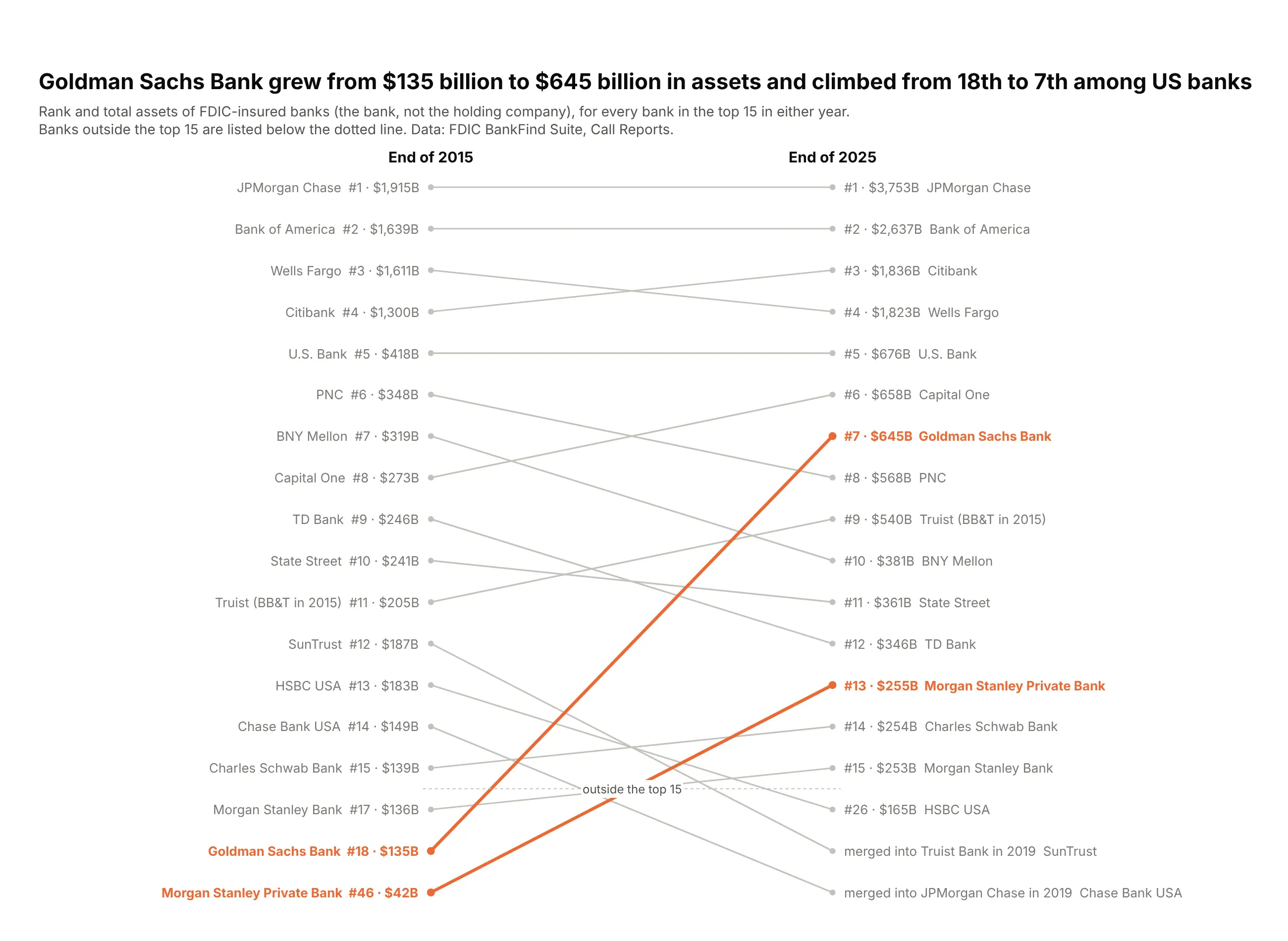
Rank slope chart of US banks by assets at the end of 2015 and 2025. Goldman Sachs Bank rises from 18th ($135B) to 7th ($645B) and Morgan Stanley Private Bank from 46th to 13th in orange; SunTrust and Chase Bank USA end as "merged" below a dotted line

Goldman Sachs Bank had $135 billion in assets in 2015 and $645 billion in 2025, climbing from 18th to 7th among US banks. Two of 2015's top 15 no longer exist. Data: FDIC BankFind Suite.

Tip: put items outside the top N below a dotted line in rank order, and label exits with what happened.

Get the data from the FDIC BankFind Suite API, Call Report total assets
(columns: bank, assets_bn_2015, rank_2015, assets_bn_2025, rank_2025, fate).

Build a rank slope chart of every bank in the top 15 in either year.
- Reverse the y axis. Banks ranked below 15 go below a dotted line, one slot each in rank order.
- Labels "#7 · $645B"; merged banks show "merged into Truist Bank in 2019".
- Goldman Sachs and Morgan Stanley Private Bank #eb6834, the rest #c3c2bc.

6. France now pays more than Italy to borrow

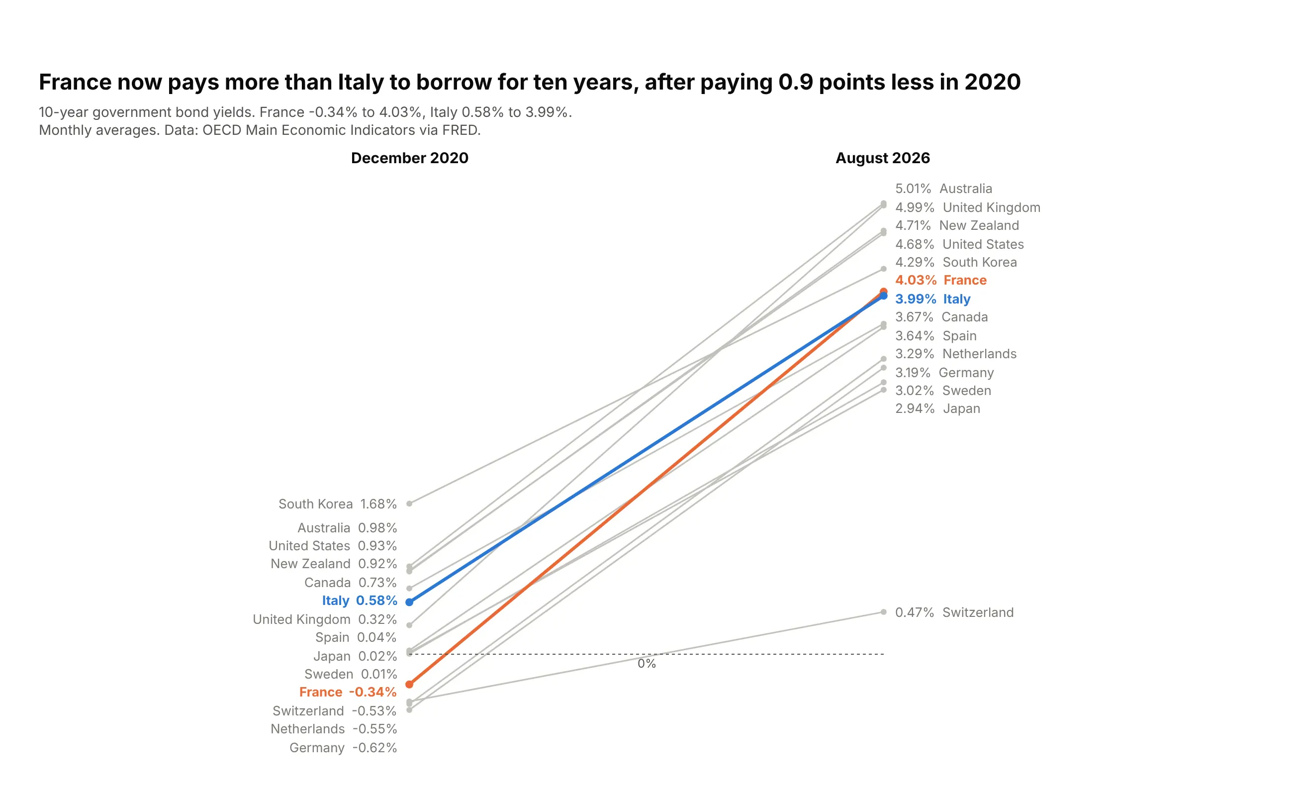
Slope chart of 10-year government bond yields in December 2020 and August 2026 in 14 countries with a dotted zero line. France rises from -0.34% to 4.03% in orange and crosses Italy, which goes from 0.58% to 3.99% in blue

In December 2020 France borrowed for ten years at -0.34% and Italy at 0.58%. By August 2026 France paid 4.03% and Italy 3.99%, so the lines cross. Data: OECD Main Economic Indicators via FRED.

Tip: draw a zero line with add_shape when some values start below zero.

Get the data from the OECD Main Economic Indicators 10-year government bond yields, via FRED (IRLTLT01xxM156N)
(columns: country, yield_2020_12, yield_2026_08; percent).

Build a plotly slope chart with a dotted zero line.
- France #eb6834, Italy #2a78d6, the rest #c3c2bc; two decimals.
- Title with the 2020 gap and the 2026 crossing.

7. Eli Lilly's revenue more than tripled

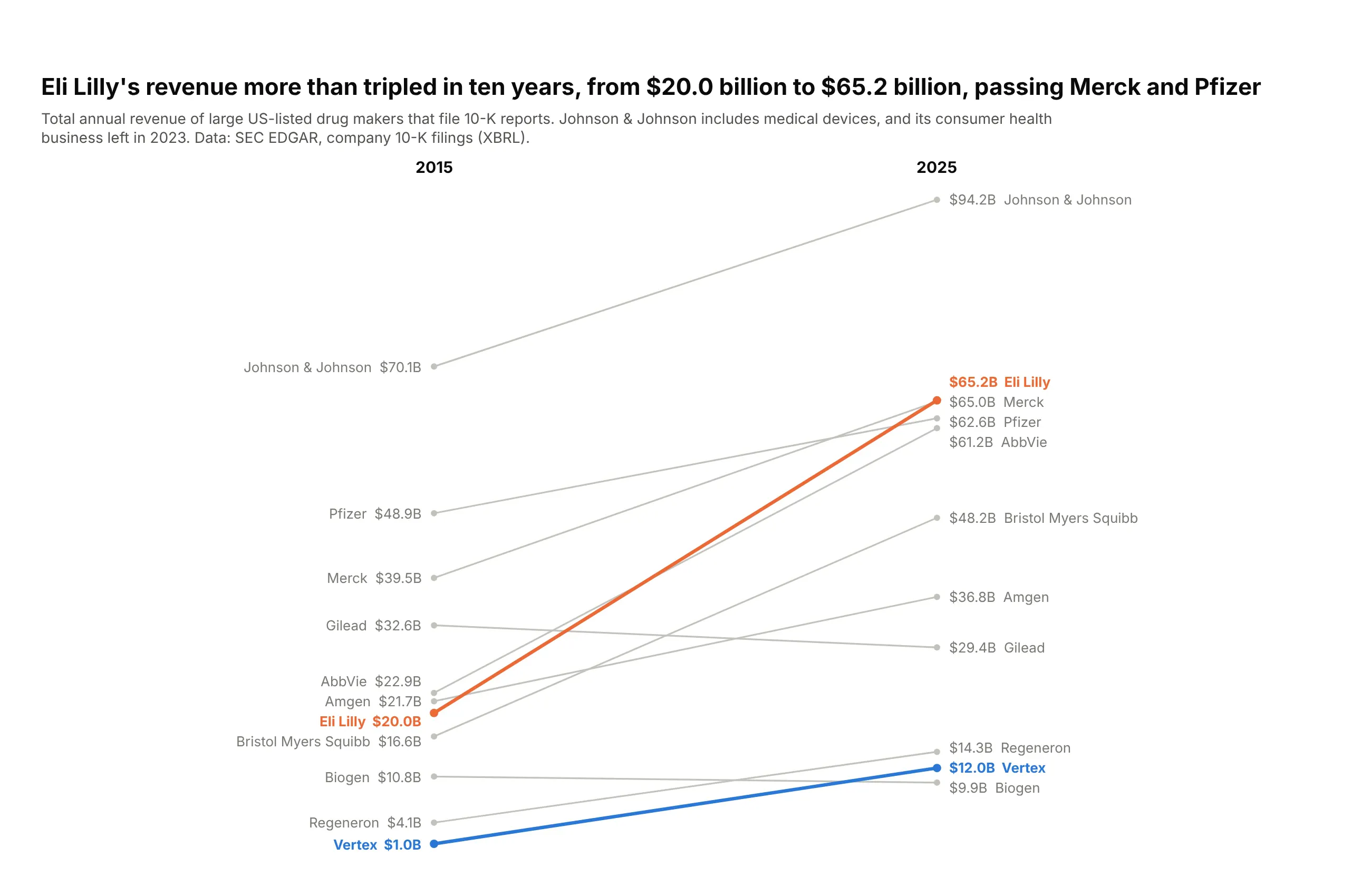
Slope chart of the revenue of 11 drug makers in 2015 and 2025. Eli Lilly rises from $20.0B to $65.2B in orange, passing Merck, Pfizer and AbbVie; Vertex rises from $1.0B to $12.0B in blue

Eli Lilly's revenue went from $20.0 billion in 2015 to $65.2 billion in 2025, passing Merck ($65.0B) and Pfizer ($62.6B). Only Johnson & Johnson, which includes medical devices, is larger. Data: SEC EDGAR, company 10-K filings.

Tip: crossings tell the ranking story without a second chart.

Get the data from SEC EDGAR XBRL company facts, total revenue from 10-K filings for calendar 2015 and 2025
(columns: company, revenue_bn_2015, revenue_bn_2025; US$ billions).

Build a plotly slope chart for 11 US-listed drug makers.
- Eli Lilly #eb6834, Vertex #2a78d6, the rest #c3c2bc; values "$65.2B".
- Subtitle notes J&J includes medical devices.

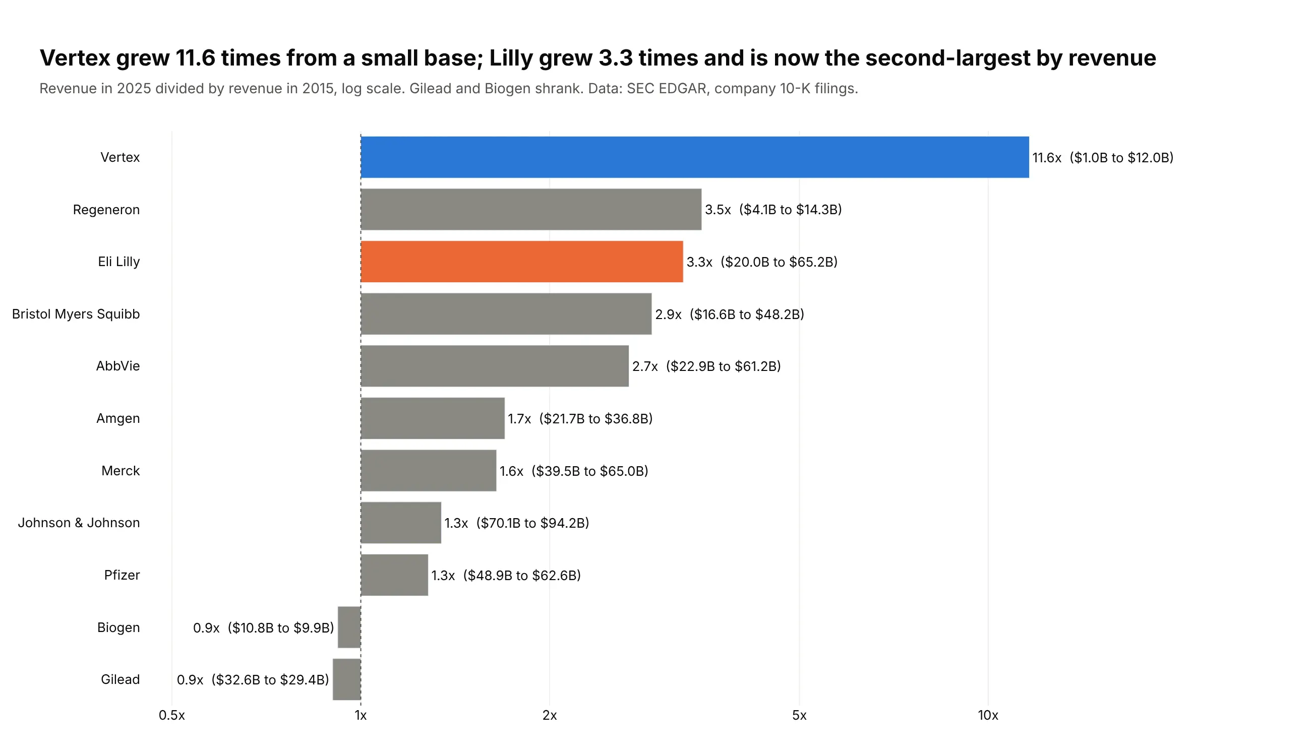
Another way to see it: a bar chart of growth multiples on a log axis, starting at 1x, ranks the growers: Vertex 11.6x, Regeneron 3.5x, Lilly 3.3x, while Gilead and Biogen shrank.

Bar chart of 2025 revenue divided by 2015 revenue on a log axis with bars starting at 1x. Vertex 11.6x in blue, Regeneron 3.5x, Eli Lilly 3.3x in orange, down to Biogen and Gilead at 0.9x

8. Dementia rose to the 5th leading cause of death

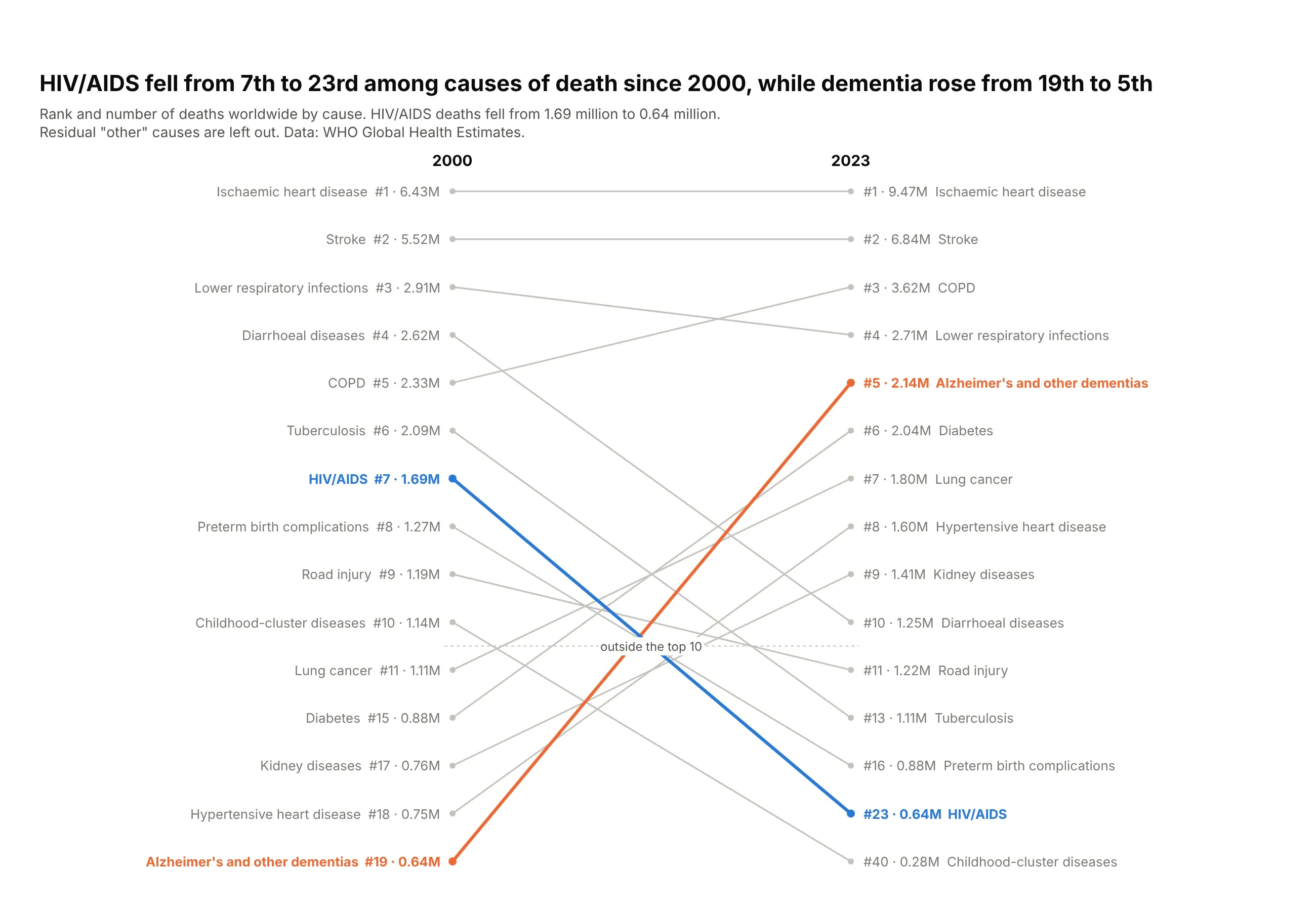
Rank slope chart of the leading causes of death worldwide in 2000 and 2023. HIV/AIDS falls from 7th (1.69M deaths) to 23rd (0.64M) in blue; Alzheimer's and other dementias rise from 19th to 5th (2.14M) in orange

HIV/AIDS was the 7th leading cause of death in 2000 and the 23rd in 2023, as deaths fell from 1.69 to 0.64 million. Alzheimer's and other dementias rose from 19th to 5th. Data: WHO Global Health Estimates.

Tip: print rank and value together ("#5 · 2.14M"), so the rank chart keeps the size.

Get the data from WHO Global Health Estimates, deaths by cause, world (xmart-api-public.who.int)
(columns: cause, deaths_2000, deaths_2023, rank_2000, rank_2023).

Build a rank slope chart of every cause in the top 10 in either year.
- Reverse the y axis; causes outside the top 10 below a dotted line.
- HIV/AIDS #2a78d6, Alzheimer's #eb6834, the rest #c3c2bc. Labels "#7 · 1.69M".

9. Bolivia lost 6.4 years of life expectancy, then regained it

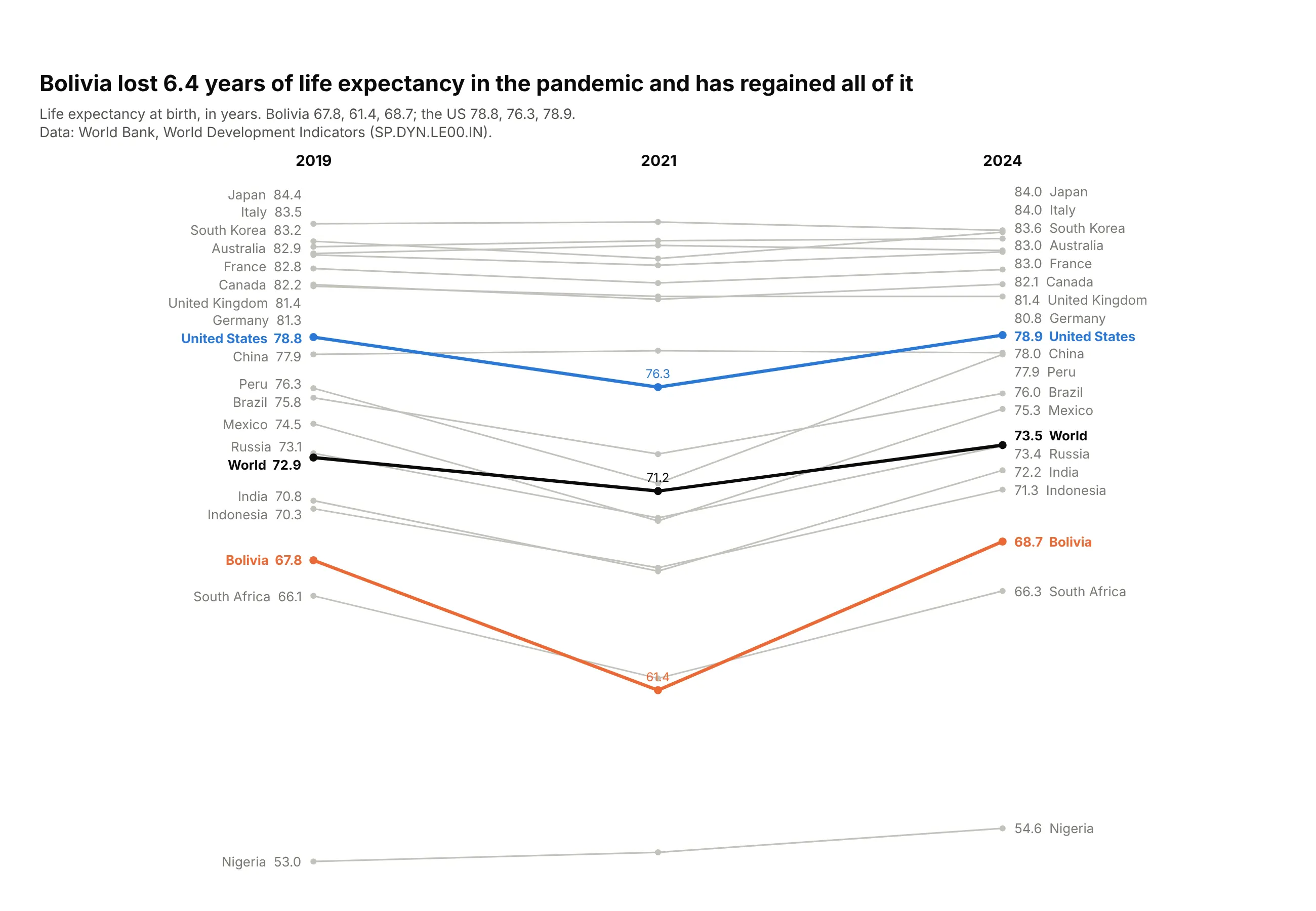
Three-column slope chart of life expectancy in 2019, 2021 and 2024 for 19 countries and the world. Bolivia drops from 67.8 to 61.4 and rebounds to 68.7 in orange; the US goes 78.8, 76.3, 78.9 in blue; the world 72.9, 71.2, 73.5 in black

Life expectancy in Bolivia fell from 67.8 years in 2019 to 61.4 in 2021, the deepest dip of these countries, and was 68.7 in 2024. The US dipped 2.5 years and recovered. Data: World Bank, World Development Indicators.

Tip: three columns make each pandemic dip a V, and its depth is the story.

Get the data from the World Bank World Development Indicators, life expectancy at birth (SP.DYN.LE00.IN)
(columns: country, le_2019, le_2021, le_2024; years).

Build a three-column plotly slope chart.
- Bolivia #eb6834, United States #2a78d6, World #0b0b0b with 2021 values printed; the rest #c3c2bc.
- Assert Bolivia has the largest 2019-2021 drop.

10. China's emissions grew almost fivefold since 1990

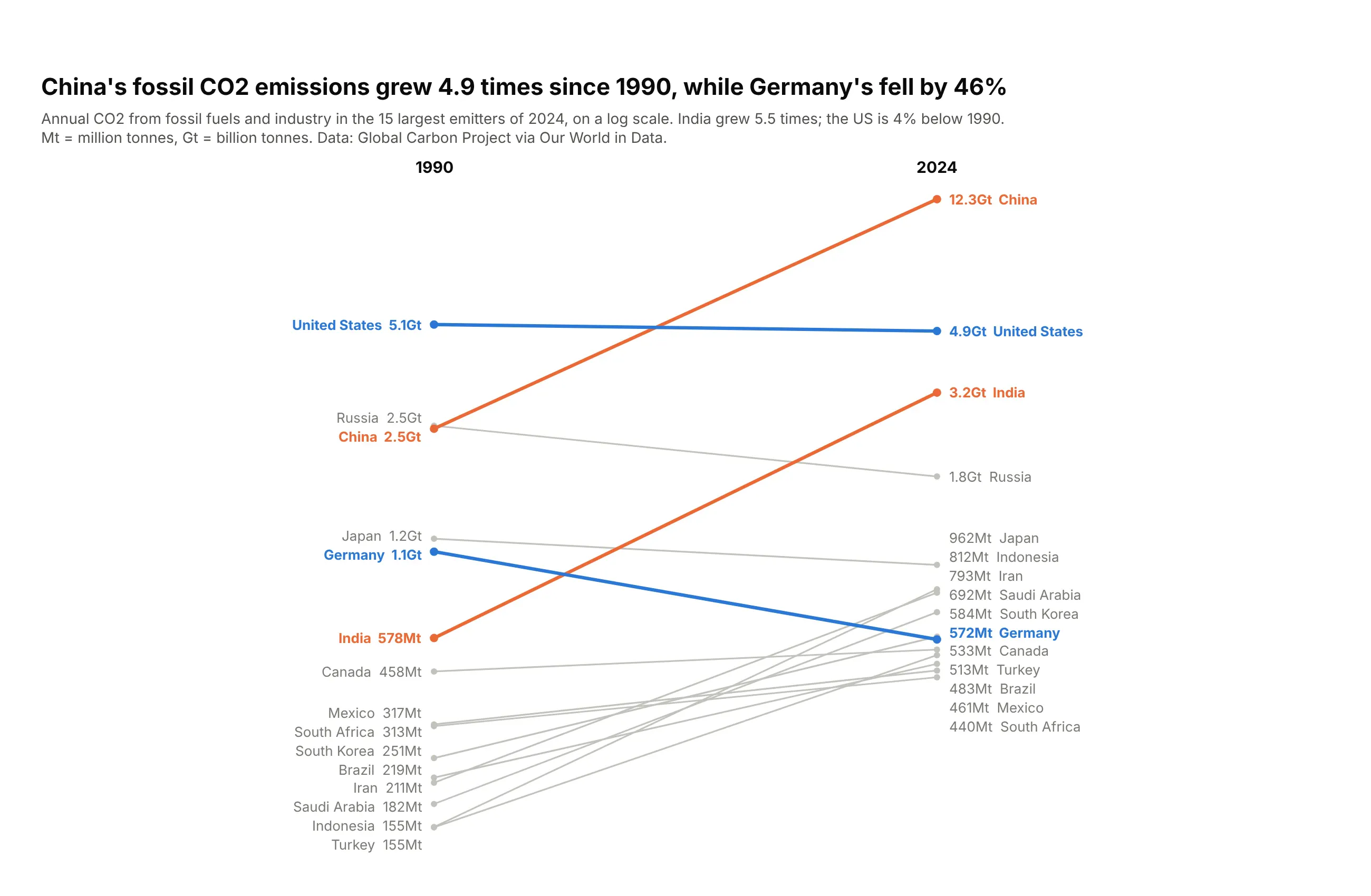
Slope chart on a log axis of fossil CO2 emissions in 1990 and 2024 for the 15 largest emitters. China rises from 2.5 to 12.3 Gt and India from 578 Mt to 3.2 Gt in orange; the US goes from 5.1 to 4.9 Gt and Germany from 1.1 Gt to 572 Mt in blue

China's fossil CO2 emissions grew 4.9 times between 1990 and 2024, to 12.3 billion tonnes. Germany's fell 46%, and the US is 4% below 1990. Data: Global Carbon Project via Our World in Data.

Tip: switch units inside one axis ("572Mt", "12.3Gt") so labels stay short.

Get the data from the Global Carbon Project via Our World in Data (github.com/owid/co2-data)
(columns: country, co2_mt_1990, co2_mt_2024; million tonnes; 15 largest emitters of 2024).

Build a plotly slope chart on a log axis, 1990 to 2024.
- China and India #eb6834, US and Germany #2a78d6, the rest #c3c2bc.
- Values over 1,000 Mt as "12.3Gt". Title with China's multiple and Germany's fall.

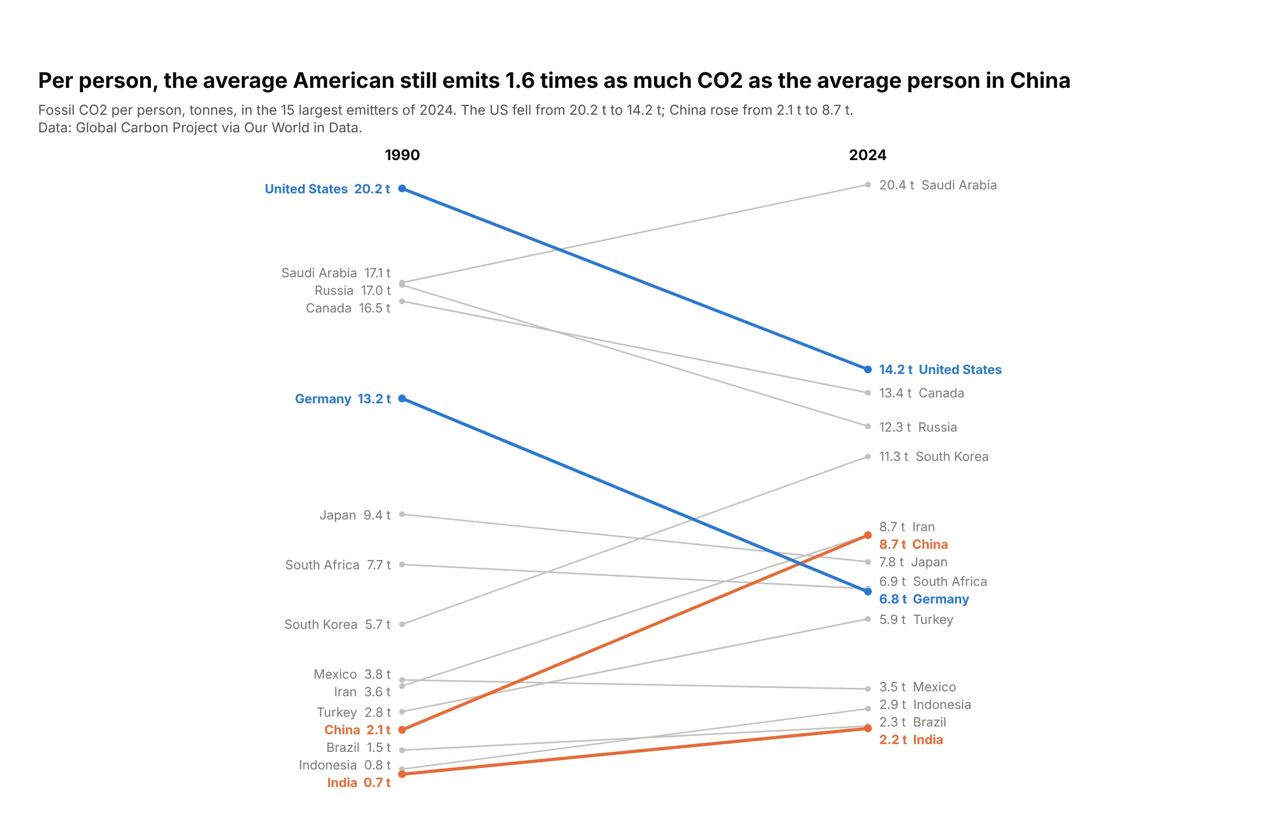
Another way to see it: per person, the order flips. The average American emits 14.2 tonnes, 1.6 times the average person in China (8.7 t).

Slope chart of CO2 per person in 1990 and 2024. The US falls from 20.2 to 14.2 tonnes and Germany from 13.2 to 6.8 in blue; China rises from 2.1 to 8.7 and India from 0.7 to 2.2 in orange