Well Log Plots - A Complete Guide

TL;DR

• A well log plot draws measurements made down a borehole against depth, with depth increasing down the page and each kind of measurement in its own column (a track), so a geologist can read across every track at one depth.
• Well log plots are also known as well logs, log plots, composite logs (when several logging runs are spliced into one record), borehole logs, and well-log strip plots, and the standard set of curves is called a triple combo. Each track is a line chart turned on its side, and a row of wells side by side is a set of small multiples.
• The standard tracks follow conventions: gamma ray with sand and shale shading, resistivity on a logarithmic scale, neutron porosity and bulk density overlaid with crossover shading, sonic slowness, and the caliper against the bit size. Together they tell sandstone from shale, how porous the rock is, and whether the pores hold water, oil, or gas.
• You can make a well log plot with Plotly from make_subplots(shared_yaxes=True) with a reversed depth axis, one go.Scatter per curve, and fill="tonextx" for the shading. lasio reads the Log ASCII Standard (LAS) files most logs come in.

What is a well log plot?

Well log plots look like this:

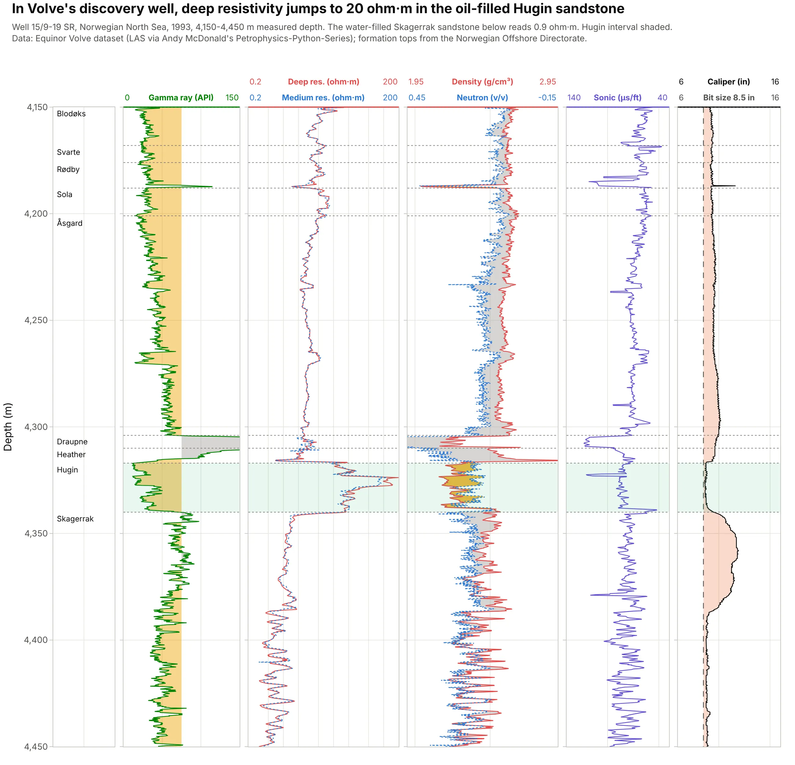
Data: Equinor’s Volve open dataset (LAS file via Andy McDonald’s Petrophysics-Python-Series); formation tops from the Norwegian Offshore Directorate.

How do you read a well log plot? In the example above, notice these things:

• Depth runs down the left axis, in meters measured along the hole, and every track shares it. This well was drilled at an angle of up to 56°, so the Hugin sandstone, 4,317 m along the hole, is 2,886 m below the drill floor.
• The gamma ray in the second track drops to a median of 27 American Petroleum Institute (API) units in the Hugin, which marks clean rock with little clay. Just above it, the Draupne Formation reads up to 304 API and runs off the track.
• In the third track, deep resistivity jumps from about 3 ohm·m in the rock above to a median of 20 ohm·m in the Hugin and falls back to 0.9 ohm·m in the Skagerrak sandstone below. Water conducts electricity and oil doesn’t, so the Hugin holds oil and the Skagerrak holds water, which is what this well found in 1993.
• In the fourth track, the density curve (solid red) crosses to the left of the neutron curve (dotted blue) in 90% of the Hugin samples, the yellow crossover shading that flags light hydrocarbons. In the shales the neutron sits to the left, shaded gray.
• The caliper in the last track stays close to the 8.5 inch bit size in the Hugin and widens to 11.9 inches in the Skagerrak, where the hole washed out.

It’s often used for charts like these:

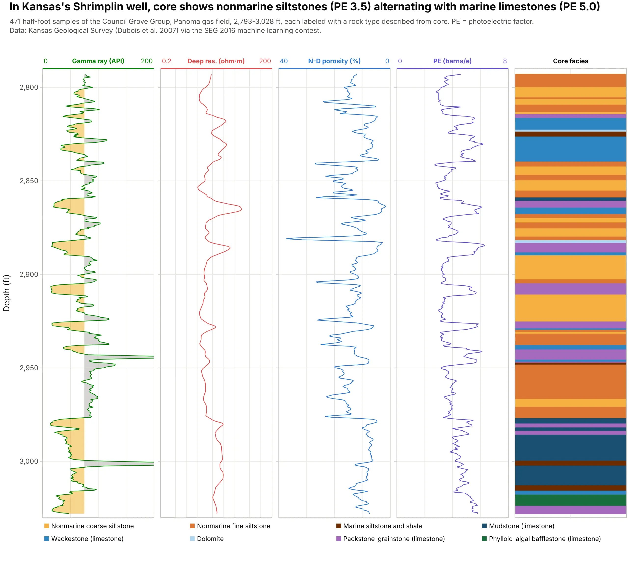
Training data for machine learning. In the Shrimplin well of Kansas’s Panoma gas field, rock types described from core sit next to the logs, and the nonmarine siltstones read a photoelectric factor (PE) of 3.5 where the marine limestones read 5.0, the kind of pattern a facies classifier learns. Data: Kansas Geological Survey (Dubois et al. 2007) via the Society of Exploration Geophysicists (SEG) 2016 machine learning contest.

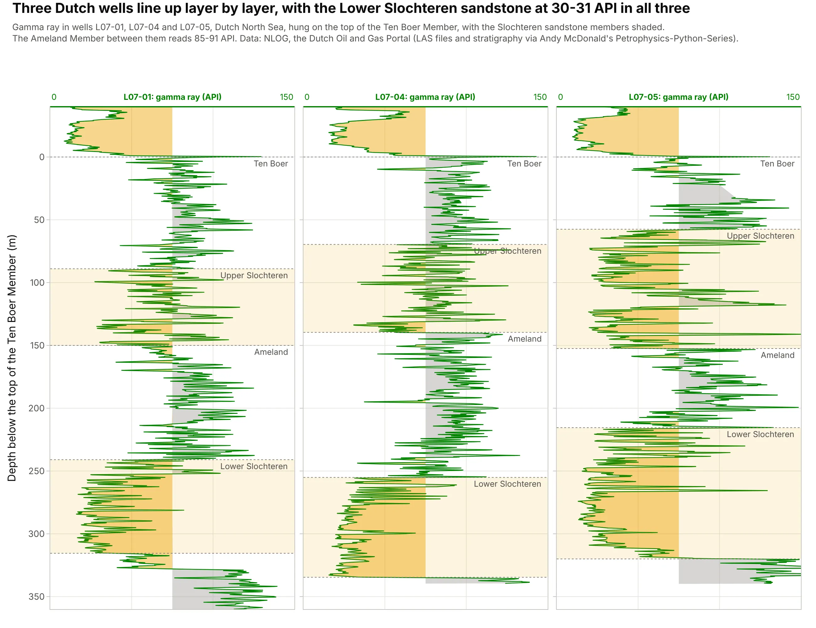
Correlating wells. Hung on a shared marker bed, three Dutch wells show the same layers, and the Lower Slochteren sandstone reads 30-31 API in all three. Data: NLOG, the Dutch Oil and Gas Portal (via Andy McDonald’s Petrophysics-Python-Series).

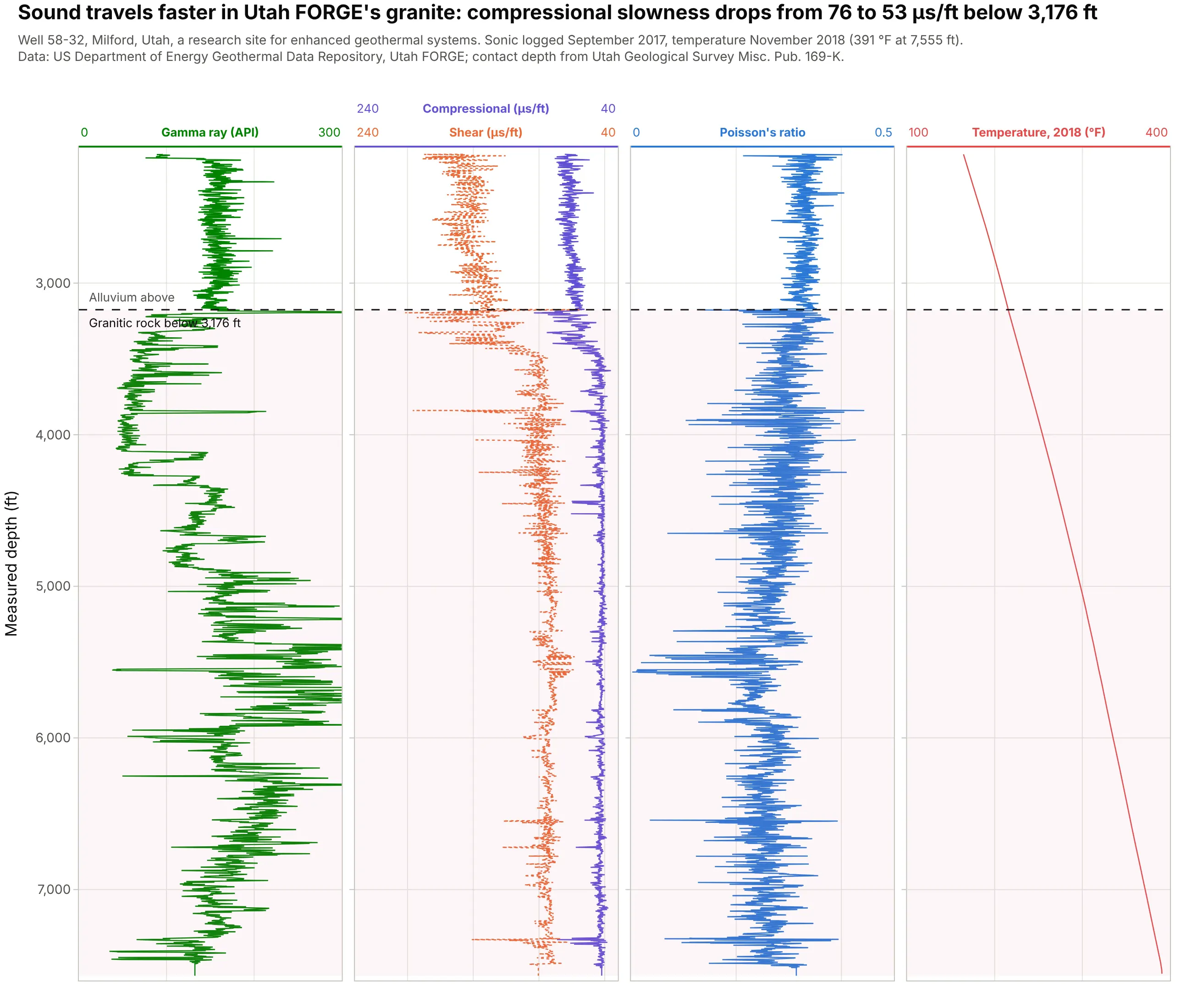
Geothermal and engineering wells. In the research well of Utah FORGE (the Frontier Observatory for Research in Geothermal Energy), compressional slowness drops from 76 to 53 microseconds per foot where the drill passed from alluvium into granite at 3,176 ft, the rock that engineers fracture to build an enhanced geothermal system. Data: US Department of Energy Geothermal Data Repository, Utah FORGE; contact depth from Utah Geological Survey Misc. Pub. 169-K.

How to read the standard curves

A well log plot assumes you know what each curve measures. Logging tools are lowered into the hole on a cable (wireline) or carried behind the drill bit, and each one measures a different physical property of the rock around the hole. These are the five you will see on almost every log, and the conventions for drawing them.

Depth goes down

Depth is on the y axis and increases downward, like the well itself, and tracks are numbered from left to right (SLB Energy Glossary). Logs are recorded against measured depth (MD), the length of the hole, which differs from true vertical depth (TVD) in any well that isn’t vertical (SLB). The Volve well above reached 4,641 m MD but only 3,132 m TVD, so say which one your axis shows.

Gamma ray: clay or clean rock

The gamma ray log measures natural radioactivity in API units, defined by a calibration pit at the University of Houston set to 200 API, “twice the radioactivity of a typical shale” (SLB). Clay minerals carry most of that radioactivity, so high readings mean shale and low readings mean clean rock. The usual shading fills yellow (sand) left of a cutoff and gray (shale) right of it. Low gamma ray means clean rock, not always sand: the marine limestones in the Kansas well above read a median of 46 API, and the granite in the FORGE well reads 156 API, the same as the sediment above it.

Resistivity: water or hydrocarbons

Resistivity tools push current into the rock. “Hydrocarbons do not conduct electricity while all formation waters do”, so the resistivity of a rock full of oil is much higher than the same rock full of water, and because the values span several orders of magnitude, the log is “usually presented on a logarithmic scale from, for example, 0.2 to 2000 ohm-m” (SLB). Tools read at several depths into the rock, and the deep reading sees past the zone where drilling fluid has soaked in (SLB). In the Volve well, two sandstones with almost the same gamma ray read 0.43 ohm·m (water) and 20 ohm·m (oil), shown in example 1 below.

Neutron and density: porosity and gas

The density tool measures bulk density in g/cm³, and the neutron tool measures hydrogen, which it reports as porosity (the share of the rock that is pore space). Both estimate porosity, and the usual display overlays them on reversed scales, density from 1.95 to 2.95 g/cm³ and neutron porosity from 0.45 to -0.15, so the curves line up when the rock is water-filled limestone. Gas has little hydrogen and low density, so the neutron reads too little porosity and the density too much, and the curves cross, “what is referred to as gas crossover” (Wikipedia):

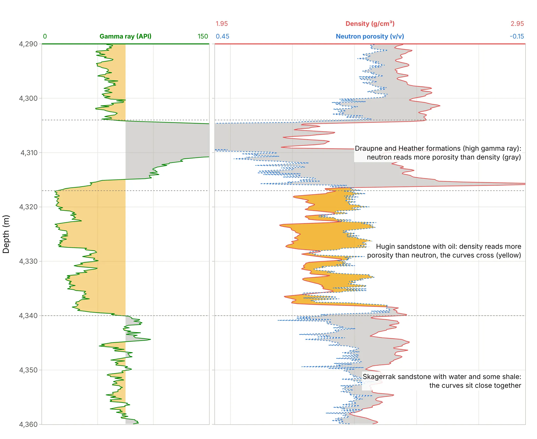
Data: Equinor’s Volve open dataset, well 15/9-19 SR.

In the shales the neutron reads more porosity than the density and sits to its left (gray). Crossover alone isn’t proof of hydrocarbons: rock types other than limestone shift the curves too, and in this well the water-filled Heimdal sandstone crosses over in 62% of its samples, against 90% in the oil-filled Hugin. That is why a geologist always reads the crossover next to the resistivity.

Sonic: how fast sound travels

The sonic log records the time sound takes to travel one foot of rock, in microseconds per foot, from about 43 in dolostone to 160 in soft shale, with steel casing at 57 (SLB). It is drawn with high values on the left, so slow, porous rock swings the same way as the neutron curve. In the FORGE well it drops from 76 to 53 where sediment gives way to granite.

Caliper: the size of the hole

The caliper measures the diameter of the hole (SLB), drawn against the size of the drill bit. Where soft rock, salt, or swelling shale has washed out (SLB), tools that press against the wall, such as the density tool, read the drilling mud instead of the rock, so the caliper tells you which readings to distrust (example 4 below).

What a geologist reads from a well log

Reading across the tracks at one depth answers three questions in turn. Gamma ray says whether the rock is sand or shale, which gives a shale volume. The density (and the neutron) say how porous it is, which gives porosity: for a quartz sandstone, porosity = (2.65 - density) / (2.65 - 1.0). Resistivity, with Archie’s 1942 equation (Archie 1942), says how much of that pore space holds hydrocarbons rather than water. Cutoffs on those numbers give the net reservoir, the thickness worth producing, which example 3 below works through.

A short history

On September 5, 1927, a Schlumberger crew lowered an electric tool into a well at Pechelbronn in Alsace, France, and recorded the first well log, a resistivity log (Wikipedia). The spontaneous potential log followed in 1931, the gamma ray log in 1939 and the neutron log in 1941, the density log in the 1950s, and in the 1970s logs that recorded resistivity and porosity in one run, today’s triple combo. G. E. Archie’s 1942 paper turned resistivity and porosity into water saturation (Archie 1942), and the Canadian Well Logging Society’s Log ASCII Standard (LAS) became the plain-text format most logs are shared in (Wikipedia). The readings of that first log aren’t published as data, so this guide shows modern logs rather than a redraw.

Alternatives to a well log plot

Here’s the same Volve interval drawn five ways. Some are better for the question, some worse, some just different:

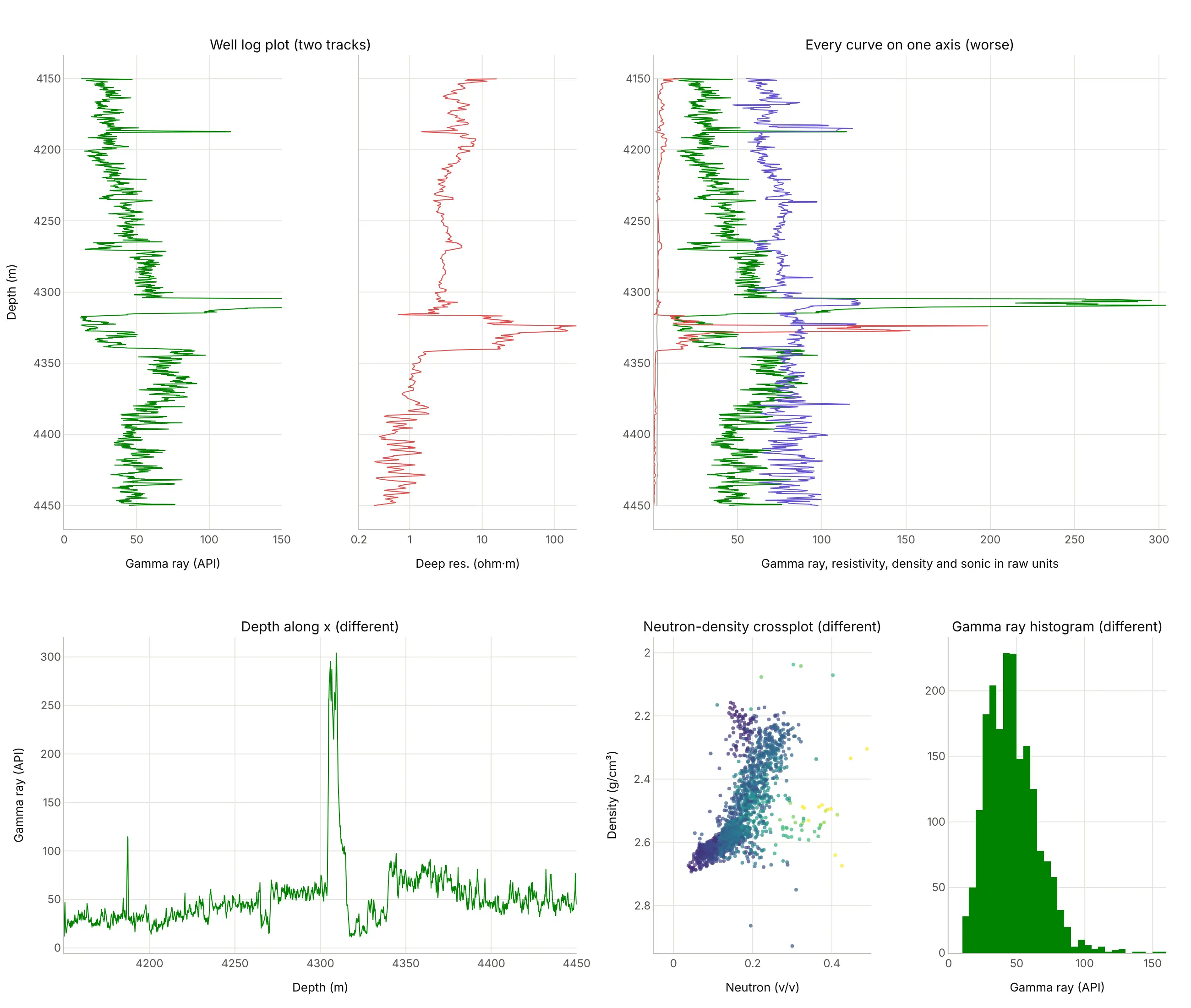
• Well log plot (the standard). Each curve gets the scale its physics needs, and all of them share depth, so you can read across at any depth.
• Every curve on one axis (worse). Resistivity (0.2 to 200) and density (2 to 3 g/cm³) flatten against the left edge next to gamma ray, so the Hugin’s resistivity jump and the density changes disappear.
• Depth along the x axis (different). It works for one curve in a slide or a report, but it breaks the convention every geologist reads in, and adding a second curve needs a second panel anyway.
• Neutron-density crossplot (different, better for rock type). Plotting neutron against density, colored by gamma ray, separates sands, shales, and carbonates into clusters, the way petrophysicists pick their parameters, but it loses depth. See the scatter plot guide.
• Histogram of gamma ray (different). It helps pick the clean and shale cutoffs for a shale volume calculation, and says nothing about where in the well they are.

How to make a well log plot

With AI

ChatGPT, Claude Code, GitHub Copilot, Cursor, and other AI tools are excellent at writing Plotly code. Name Plotly in the prompt, and spell out the conventions, because a model will otherwise draw depth upward and resistivity on a linear scale:

With Plotly Studio

Plotly Studio is a desktop app where you point an AI at a dataset and it builds charts and a Dash app around your questions. Ask for a well log plot the same way:

Show a well log plot of the selected well with gamma ray, resistivity on a log scale, and neutron-density with crossover shading, depth increasing downward, the formation tops as lines, and a dropdown to pick the well.

Make a well log plot in Python or JavaScript

This is the code AI tools write under the hood. Plotly has no dedicated well log trace, so a well log plot is a row of subplots with a shared, reversed depth axis and one go.Scatter per curve with x = value and y = depth. Shading uses pairs of traces with fill="tonextx", which fills sideways to the previous trace:

In JavaScript, plotly.js draws the same thing with a two-column grid and a shared y axis:

Share it

Every Plotly chart has a Share chart button (the cloud icon in its toolbar) that uploads it to Plotly Cloud and gives you a link. Only you can see it until you change its visibility.

For a live app, put the chart in a Dash app and publish it with the Plotly Cloud CLI. Coding agents can run these commands for you:

If your data has to stay in your own cloud or data center, publish to Dash Enterprise instead.

Dos and don’ts

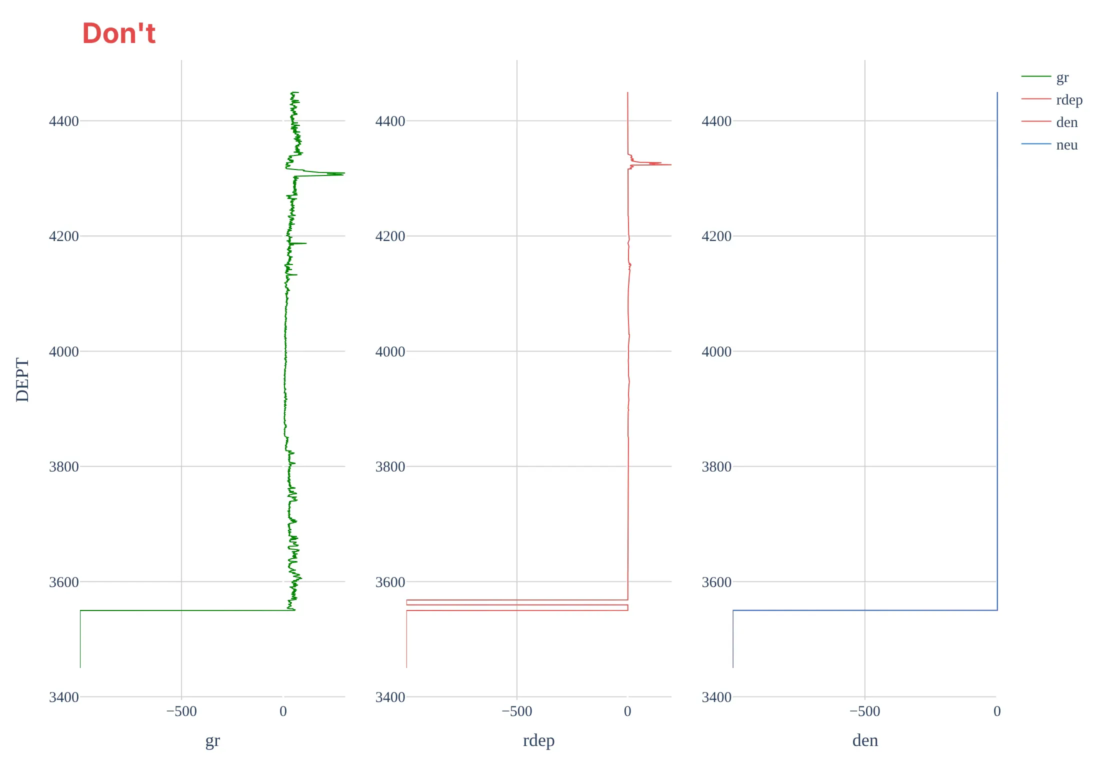
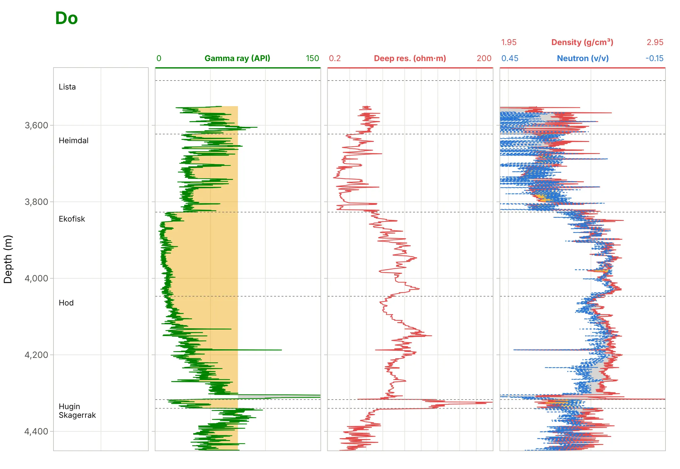
Most mistakes in well log plots come from plotting a LAS file as it is, without the field’s conventions. Here is the Volve well from 3,450 to 4,450 m both ways, with the same curve colors.

Don’t plot the LAS null value (-999.25) as data, let depth increase upward, give each panel its own depth axis, draw resistivity on a linear scale (here a single 200 ohm·m reading squashes everything else), or keep raw mnemonics, a legend, and a serif font:

Do leave the nulls as gaps, draw depth down one shared axis, put resistivity on a log scale, label each track’s scale in a header, shade the gamma ray and the crossover, and mark the formation tops:

Checklist

Do

• Put depth on the y axis, increasing downward, shared by every track, and say whether it is MD or TVD.
• Use the field’s scales: resistivity on a log scale, neutron and density overlaid on reversed scales, and sonic with high values on the left.
• Write each curve’s name, units, and scale ends above its track, in the curve’s color.
• Draw the caliper with the bit size, and treat readings where the hole washed out with suspicion.
• Mark formation tops across all tracks, and hang wells on a marker bed when you correlate them.

Don’t

• Plot -999.25 or other null values; convert them to missing values (lasio does).
• Mix feet and meters, or MD and TVD, between wells on one plot.
• Read crossover, or low gamma ray, as proof on its own; check it against the other tracks.
• Squeeze more than five or six tracks into one image; split them into two figures instead.

Options to customize

A well log plot in Plotly is a set of subplots and go.Scatter traces, so these are the options that matter most. The full lists are in the subplots documentation and the scatter trace reference.

1. make_subplots(rows=1, cols=n, shared_yaxes=True): one track per column, all on one depth axis.
2. column_widths: wider tracks for overlays such as neutron-density, narrow ones for a formation or facies column.
3. fig.update_yaxes(autorange="reversed"), or range=[bottom, top]: depth increasing downward.
4. fig.update_xaxes(type="log", range=[np.log10(0.2), np.log10(2000)]): resistivity and permeability tracks. Log axis ranges are given in powers of ten.
5. fill="tonextx" on a pair of traces: shading between a curve and a cutoff, or between two curves, sideways to the previous trace.
6. xaxis.side="top" or header annotations: put the scales above the tracks, where log readers expect them.
7. line.dash: tell two curves in one track apart (solid density, dotted neutron).
8. fig.add_hline(y=..., row=1, col=...) and fig.add_hrect: formation tops and shaded zones across every track.
9. hovermode="y unified": one hover label with every curve’s value at the depth under the mouse.
10. go.Heatmap in a narrow track: a categorical column such as core facies or lithology.

More well log plot examples

Six more well log plots built from real public data, each with its source, the technique that makes it work, and a prompt to rebuild it.

1. Two sandstones, one with water and one with oil

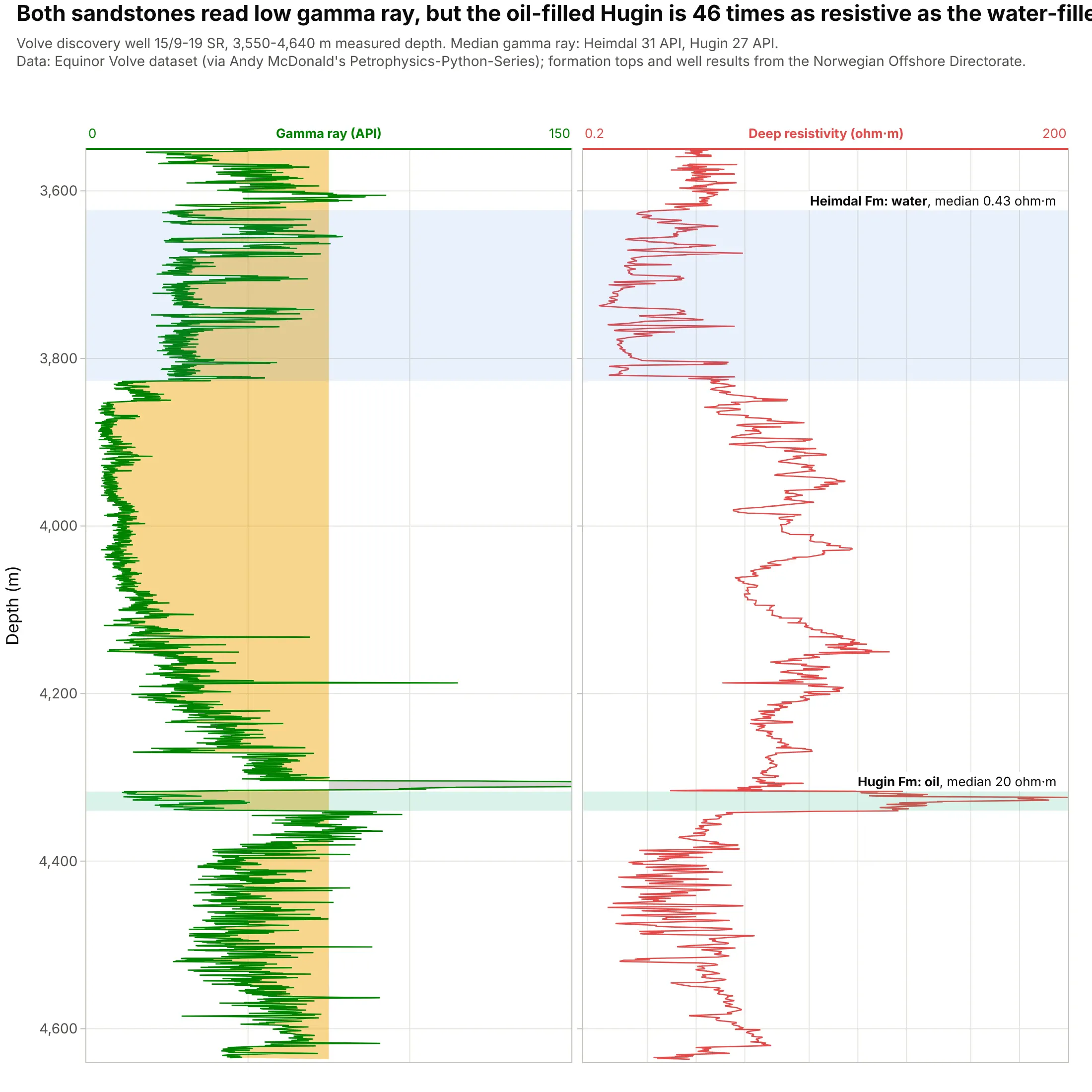
The Heimdal and Hugin sandstones read almost the same gamma ray (31 and 27 API), but the oil-filled Hugin is 46 times as resistive as the water-filled Heimdal, 20 against 0.43 ohm·m. The well was drilled to test gas in the Heimdal, which turned out wet, and found the Volve oil field in the Hugin instead. Data: Equinor’s Volve open dataset; well results from the Norwegian Offshore Directorate.

Tip: shade and label the intervals you want compared, so the reader looks across the tracks at the right depths.

2. A composite log of the whole well

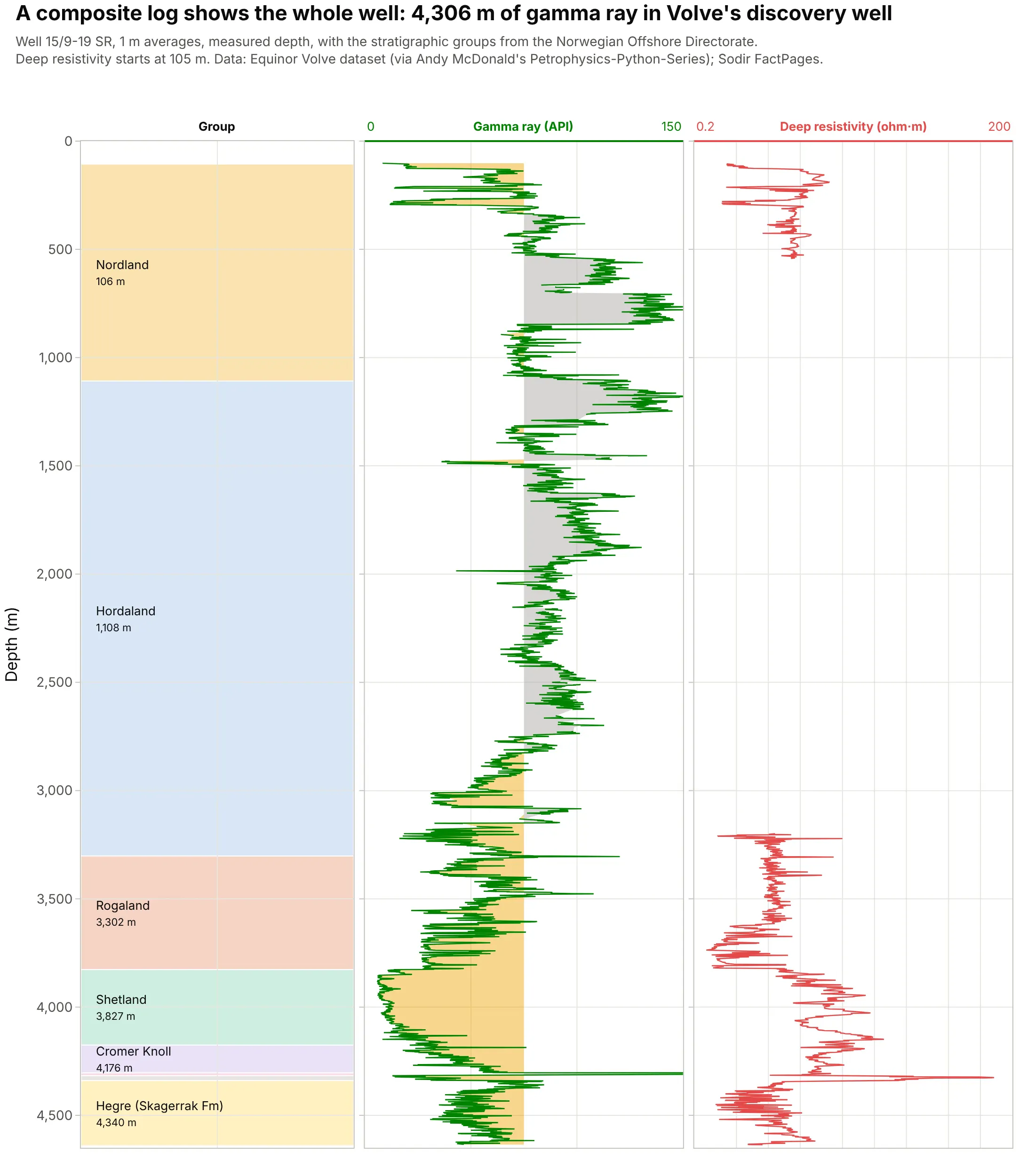
A composite log splices every logging run into one record of the well (SLB), here 4,306 m of gamma ray from 102 m to 4,636 m next to the stratigraphic groups. It is the overview a geologist scans before zooming into a reservoir. Data: Equinor’s Volve open dataset; groups from the Norwegian Offshore Directorate.

Tip: average long logs to one value per meter before plotting the whole well, and keep the full resolution for the zoomed views.

3. From logs to net reservoir

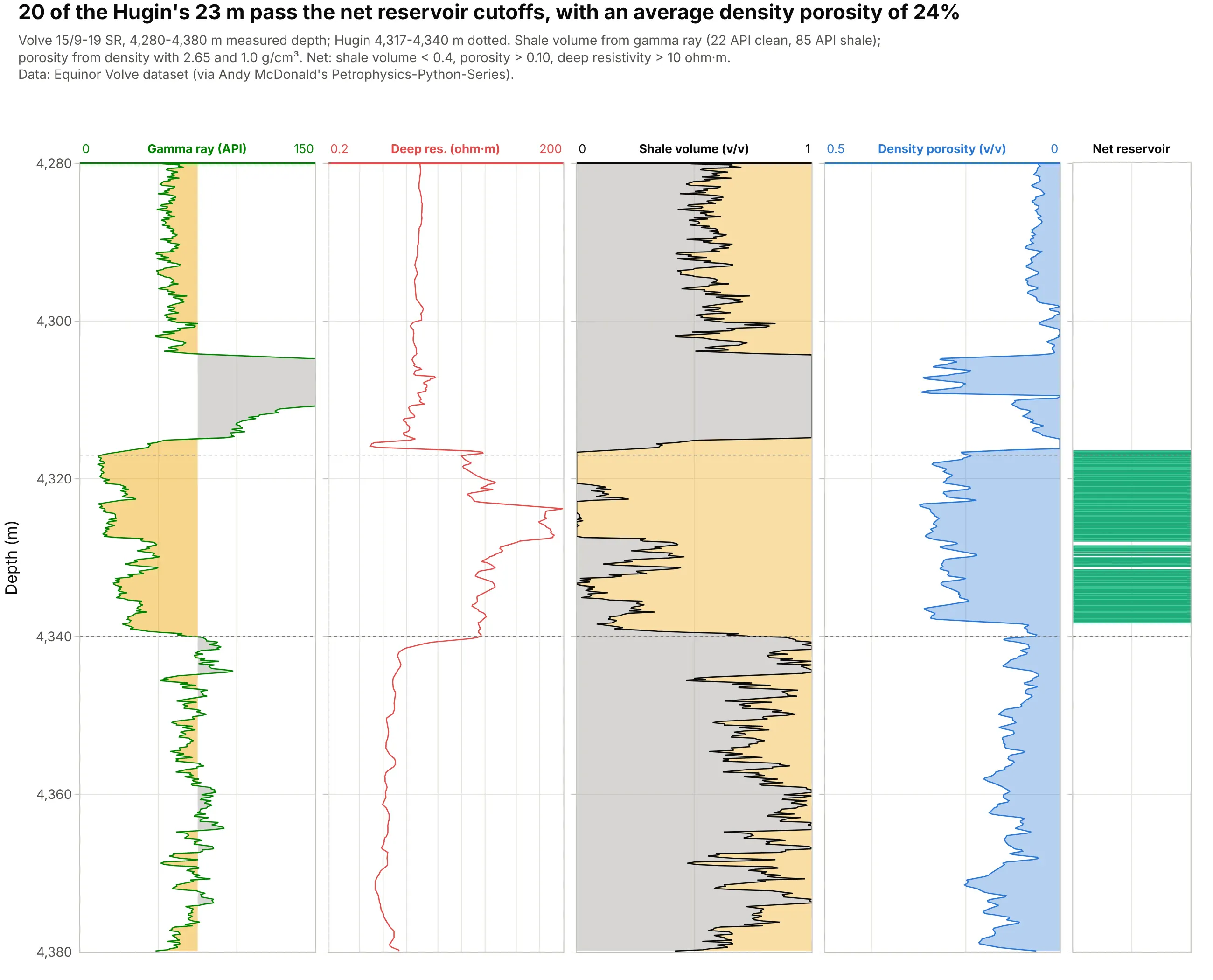
Turning gamma ray into shale volume and density into porosity, then applying three cutoffs, gives 20 m of net reservoir in the 23 m Hugin, with an average density porosity of 24%. The cutoffs here are common starting points rather than the operator’s, so they are written on the chart. Data: Equinor’s Volve open dataset.

Tip: put computed curves next to the raw logs they come from and print the parameters in the subtitle, so anyone can check the answer.

4. Where the hole washed out, the density log measures mud

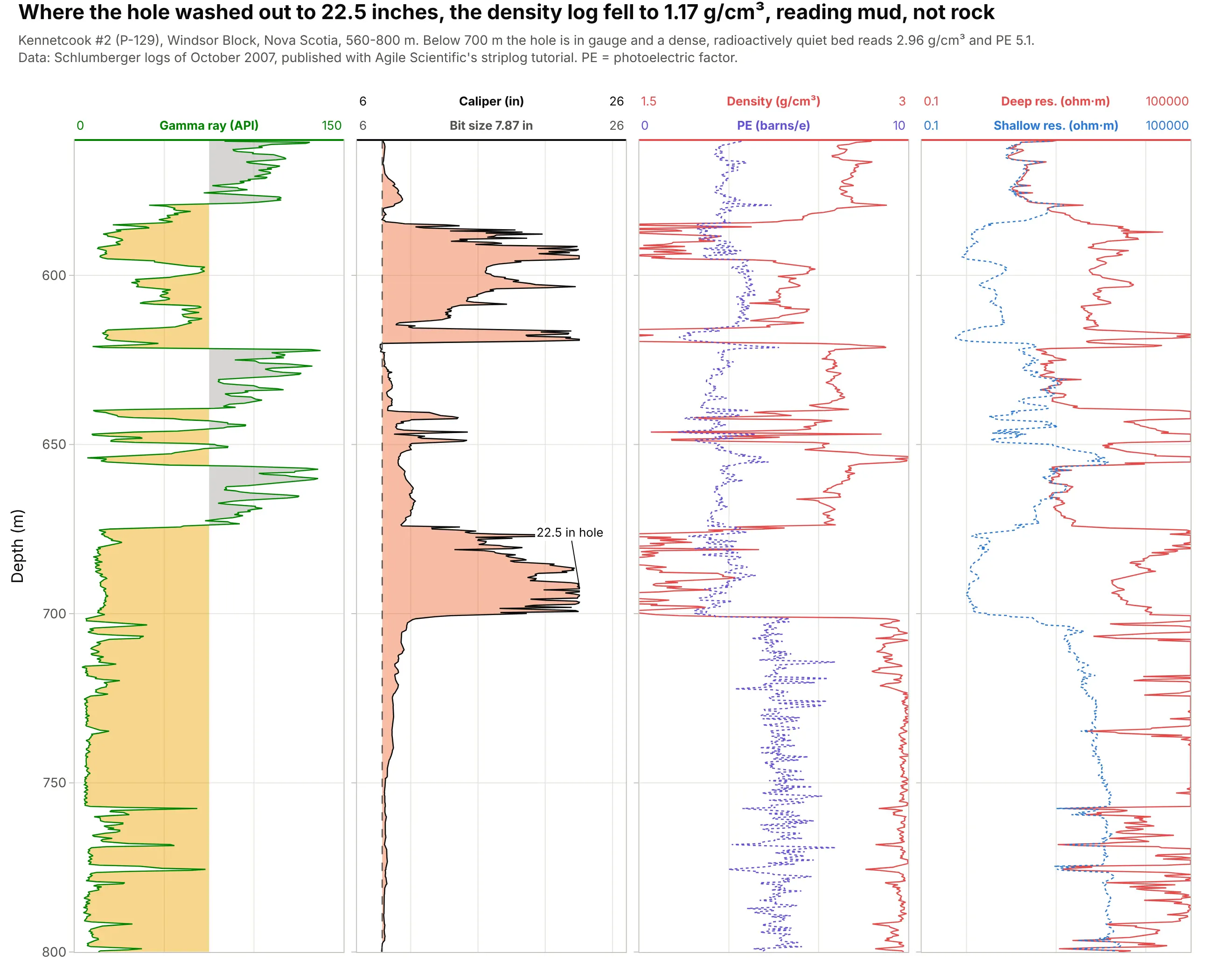
Between 580 and 700 m the hole in this Nova Scotia well widened to 22.5 inches around a 7.87 inch bit, and the density log read as low as 1.17 g/cm³, which is the drilling mud, not the rock. Below 700 m the hole is in gauge and the logs read a dense, quiet bed at 2.96 g/cm³. Data: Kennetcook #2 (P-129), Schlumberger logs of October 2007, via Agile Scientific’s striplog tutorial.

Tip: shade the caliper wherever it is wider than the bit, so washouts jump out before anyone interprets the density.

5. A geothermal well warming back up after drilling

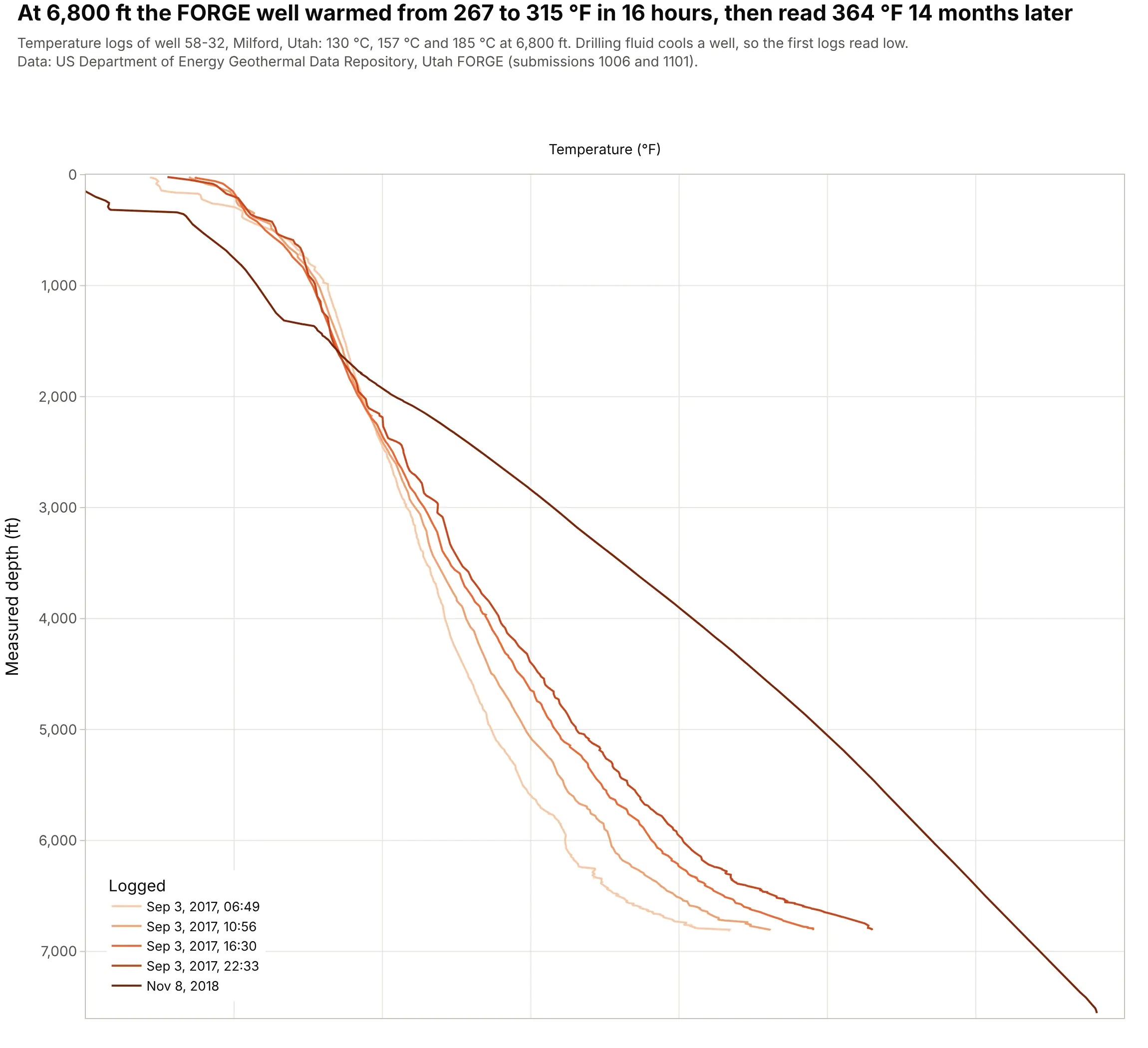
Drilling fluid cools the rock around a well (SLB), so four temperature logs run on the day drilling stopped show the bottom of the well warming from 267 to 315 °F in 16 hours. A log 14 months later read 364 °F at the same depth. Data: US Department of Energy Geothermal Data Repository, Utah FORGE (submission 1006 and 1101).

Tip: overlay repeat logs of one well in one track with a sequential color ramp from the first run to the last.

6. A drilling log: the bit slows down in granite

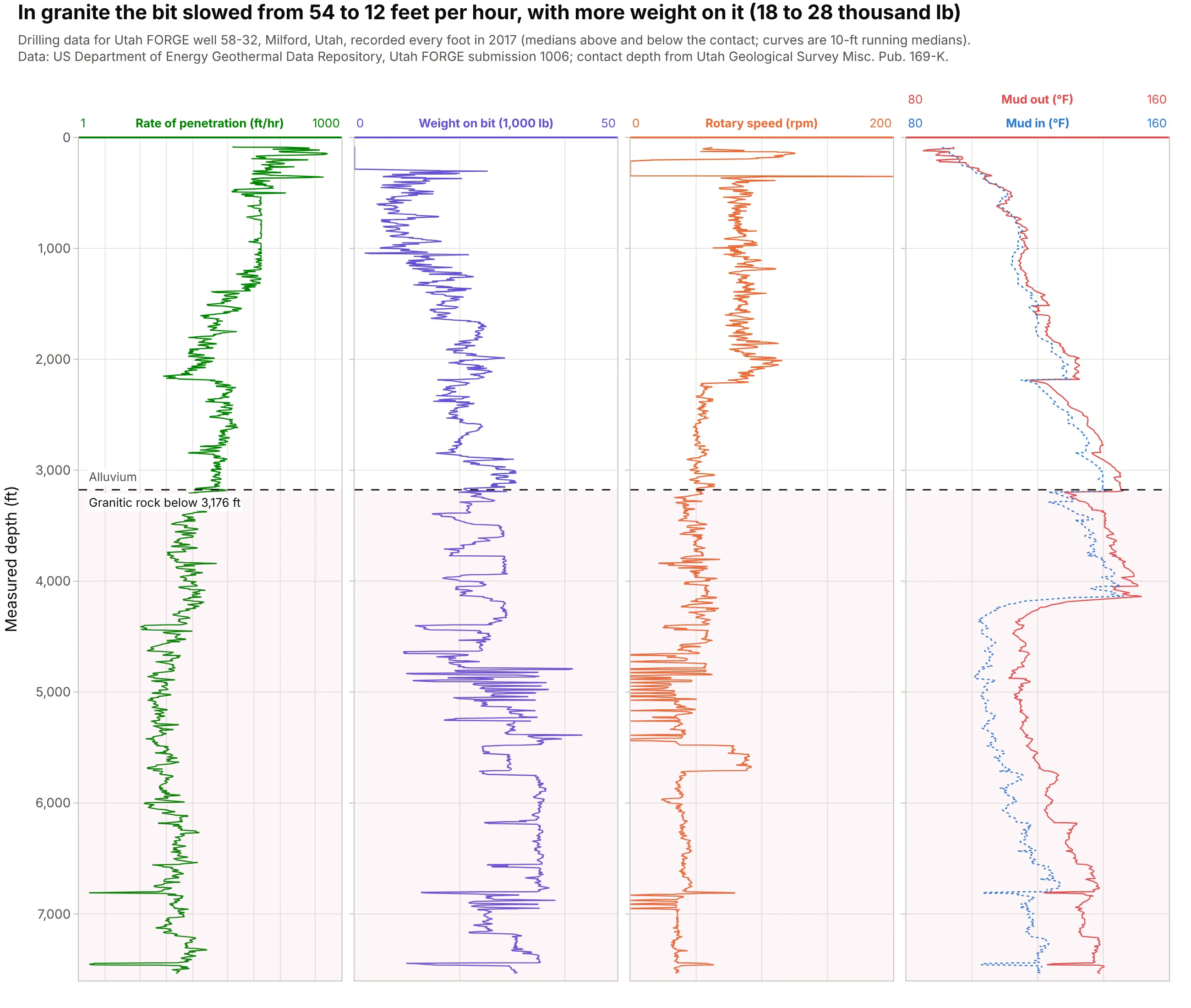
Drilling data recorded every foot reads like any other log: in the FORGE well the bit cut 54 feet per hour in alluvium and 12 in granite, even with weight on the bit raised from 18,000 to 28,000 lb. Drilling engineers read these tracks to plan bits and spot problems. Data: US Department of Energy Geothermal Data Repository, Utah FORGE.

Tip: put rate of penetration on a log scale, because it swings from a few feet to hundreds of feet per hour.