Chris Parmer

November 7, 2026

Striplogs - A Complete Guide

TL;DR

A striplog draws what a well went through as a column of rock types (lithology) against depth, each interval filled with a pattern for its rock type, usually from descriptions of core or drill cuttings. Next to measured log curves on the same depth axis it becomes a composite log.
Striplogs are also known as strip logs, lithology logs, lithologic columns, and borehole logs, and a set of wells side by side is a well correlation panel or, drawn as a network in perspective, a fence diagram. They are related to well log plots, which show the measured curves, and to small multiples.
The fills follow the US Federal Geographic Data Committee (FGDC) and US Geological Survey (USGS) lithology convention: dots for sandstone, dashes for shale and siltstone, and a brick-like grid for limestone. Plotly’s built-in marker.pattern shapes approximate it closely.
You can make a striplog with Plotly from horizontal go.Bar traces, one bar per bed, in make_subplots(shared_yaxes=True). Shapes that reference two axes at once (plotly.js 3.4 and later) link the same formation top between wells, and the links follow when you pan one well’s depth axis.

What is a striplog?

Striplogs look like this:

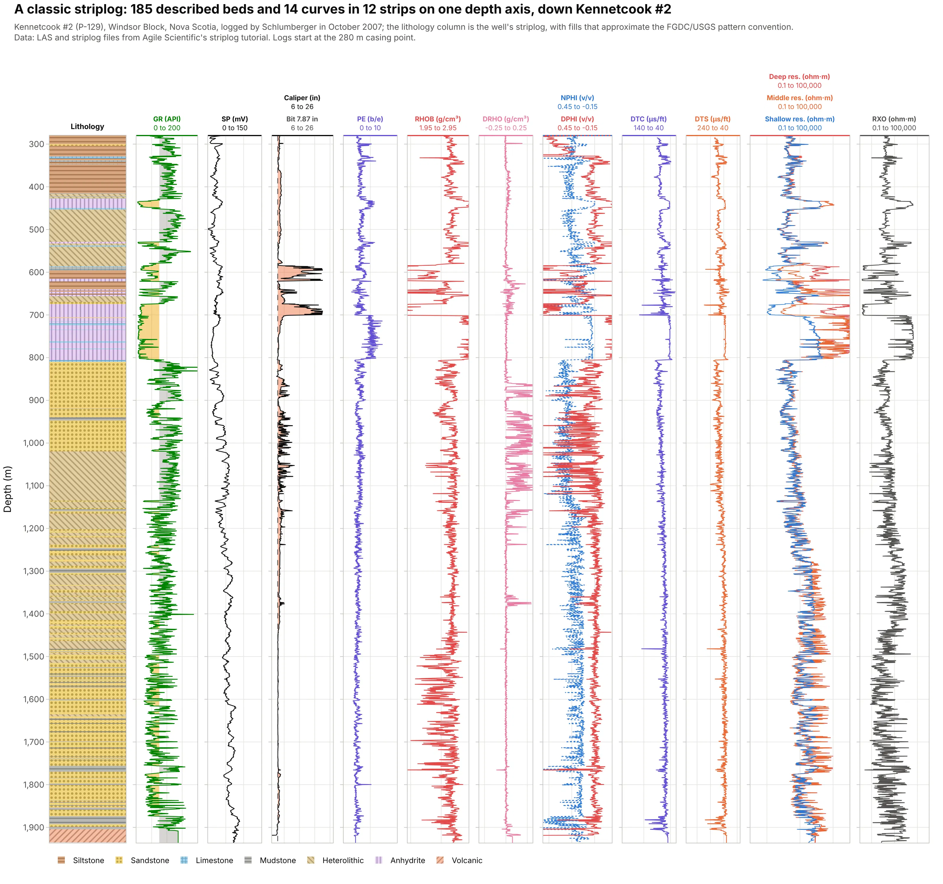
A twelve-strip striplog of Kennetcook #2 in Nova Scotia from 280 to 1,935 m: a lithology column with patterned fills for siltstone, sandstone, limestone, mudstone, heterolithic rock, anhydrite, and a volcanic bed at the base, then gamma ray, spontaneous potential, caliper, photoelectric factor, bulk density, density correction, neutron and density porosity, compressional and shear sonic, three laterolog resistivities on a log scale, and flushed-zone resistivity, all on one depth axis

Data: Kennetcook #2 (P-129), Schlumberger logs of October 2007 and the well’s striplog, from Agile Scientific’s striplog tutorial.

How do you read a striplog? In the example above, notice these things:

The first column is the lithology: 185 described beds from 280 to 1,935 m, each a rectangle from its top to its base, filled with the pattern for its rock type. Sandstone, with dots, adds up to 640 m, the most of any rock type.
The other eleven strips are measurements on the same depth axis: gamma ray, spontaneous potential (SP), caliper, photoelectric factor (PE), bulk density and its correction, neutron and density porosity, compressional and shear sonic, and four resistivities. Each strip has its own scale in its header.
Reading across at one depth checks the description against the logs. The lavender anhydrite beds between about 700 and 810 m read low gamma ray, high density, and resistivity at the 100,000 ohm·m ceiling of the tool.
The caliper strip shows the hole washing out above 700 m, where the density log reads the drilling mud rather than the rock.

It’s often used for charts like these:

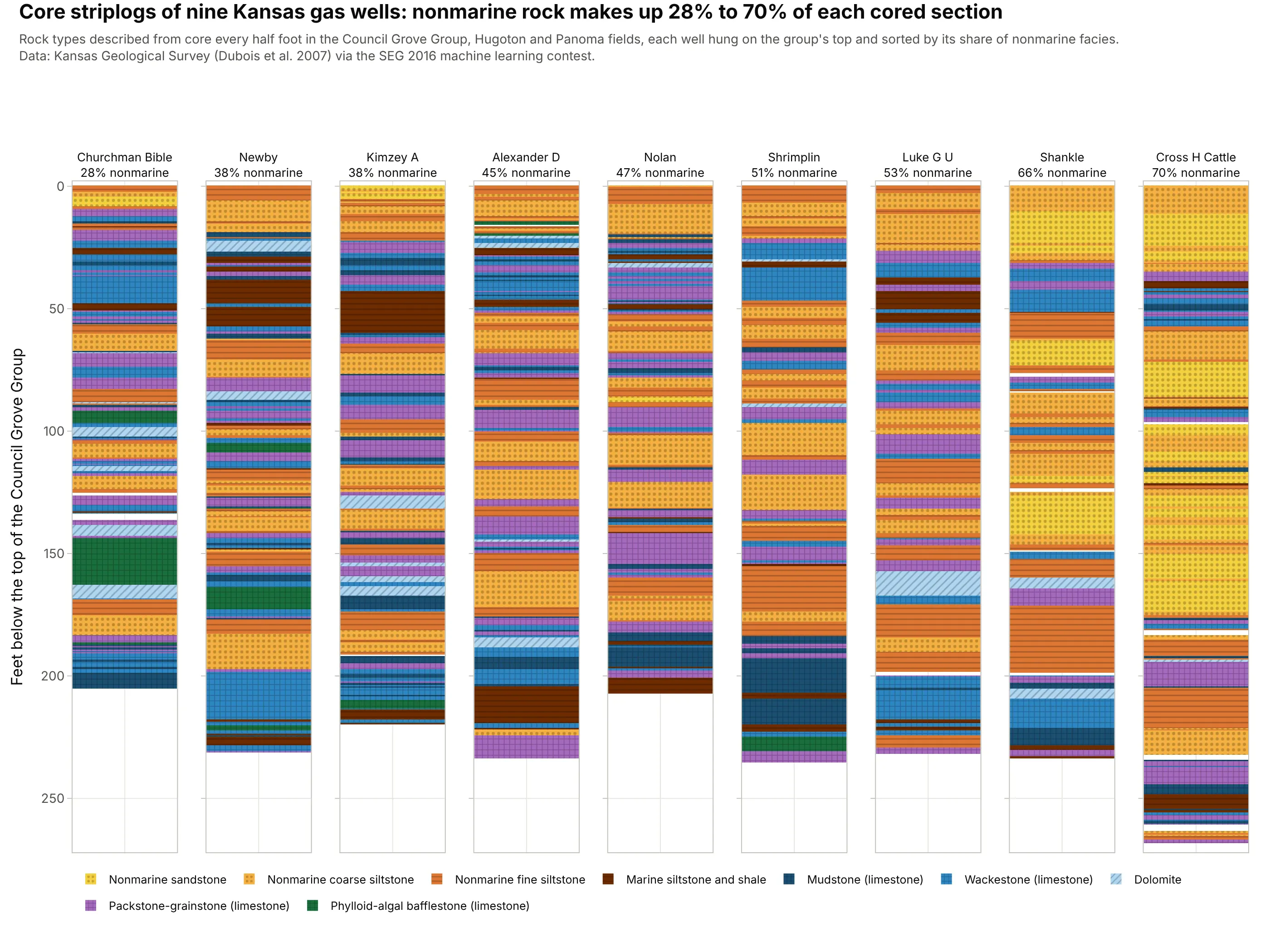
Nine side-by-side core striplogs of Kansas gas wells, each hung on the top of the Council Grove Group and colored by nine facies from nonmarine sandstone and siltstones in yellows and oranges to marine limestones in blues, purples, and green, sorted from 28% to 70% nonmarine

Core descriptions for machine learning. Nine Kansas gas wells with a rock type described from core every half foot, the training set of a well-known machine learning contest, show nonmarine rock making up 28% to 70% of each cored section. Data: Kansas Geological Survey (Dubois et al. 2007) via the Society of Exploration Geophysicists (SEG) 2016 machine learning contest.

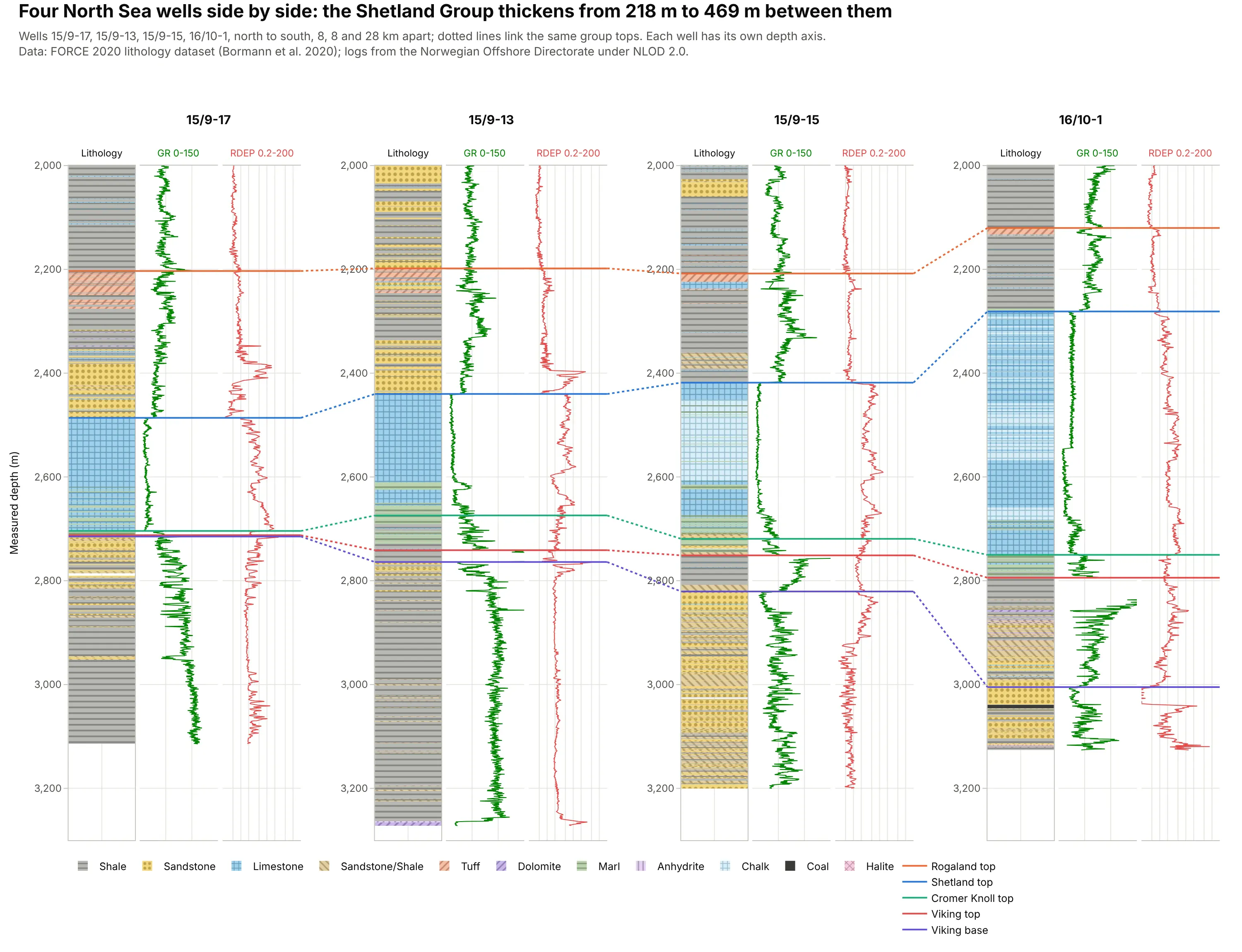
A fence diagram of four North Sea wells, 15/9-17, 15/9-13, 15/9-15, and 16/10-1, each with a lithology column, gamma ray, and deep resistivity on its own depth axis, with colored lines at five group tops in each well and dotted links joining the same top between neighbouring wells

Correlating wells in a fence diagram. Four North Sea wells side by side, with dotted links between the same group tops, show the Shetland Group thickening from 218 m to 469 m. Data: FORCE 2020 lithology dataset (Bormann et al. 2020); logs from the Norwegian Offshore Directorate under the Norwegian Licence for Open Government Data (NLOD 2.0).

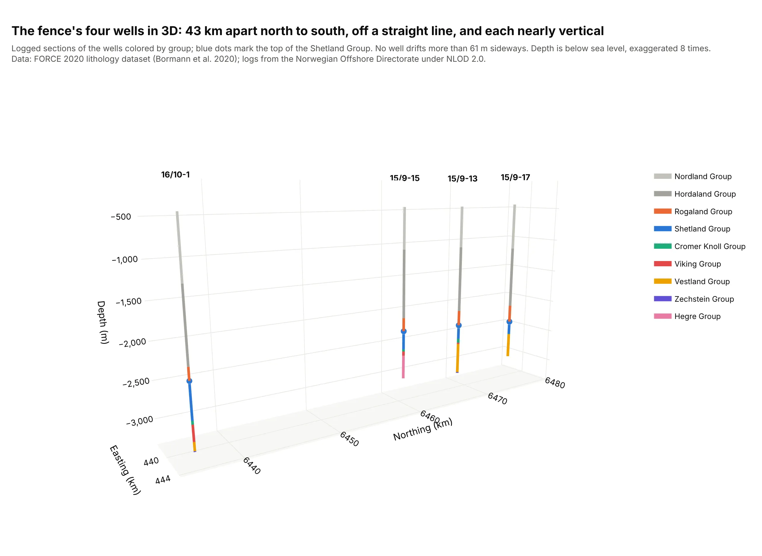
The same four wells as 3D lines colored by group against easting, northing, and depth below sea level, spread 43 km north to south with blue dots at the top of the Shetland Group

Showing where the wells really are. A fence lays wells side by side as if they stood in one plane, so a 3D view of the same four wells, 43 km apart and off a straight line, belongs next to it. Data: FORCE 2020 lithology dataset (Bormann et al. 2020).

Striplog, well log or composite log?

The three names describe what is in the columns:

A well log is “the measurement versus depth or time, or both, of one or more physical quantities in or around a well” (SLB Energy Glossary): gamma ray, resistivity, density, and so on, recorded by tools on a cable or behind the drill bit. The well log plot guide covers how to read and draw those curves.
A striplog is a column of intervals, each with a top, a base, and a description, usually of the rock seen in core or cuttings. Agile Scientific built its open-source striplog library with the Nova Scotia Department of Energy to digitize “cuttings and core descriptions” and “hand-drawn striplog images” (Agile Scientific), the source of the Kennetcook column above. The intervals can hold any label: rock type, formation, facies, or grain size.
A composite log splices several logs into one record of the well (SLB), and in practice it is the sheet with the lithology column and the measured curves on one depth axis, like the Kennetcook example.

Side by side, the logs of several wells make a well correlation panel. SLB defines a fence diagram as cross sections “displayed in a network” in “two-dimensional perspective view” (SLB); the flat row of wells in this guide is the simplest version, and the 3D view stands in for the perspective.

How the lithology patterns work

Geologic maps and stratigraphic columns in the US use the patterns of the FGDC Digital Cartographic Standard for Geologic Map Symbolization, published by the USGS as Techniques and Methods 11-A2; its section 37 numbers the lithologic patterns, for example 607 for massive sandstone, 616 for siltstone, 620 for clay shale, 627 for limestone, and 642 for dolostone (USGS). Colors are optional, and many companies add their own.

Plotly’s bar traces take a marker.pattern with eight shapes (., -, +, /, \, x, | and none), which approximate the FGDC patterns closely: dots for sandstone, dashes for siltstone and shale, a grid for limestone and chalk, slanted lines for dolostone, and crosses for granite. The examples here use these fills:

Sandstone: dots, like FGDC pattern 607, on yellow (.).
Siltstone, shale and mudstone: dashes, like 616 and 620, on tan or gray (-).
Limestone and chalk: a brick-like grid, like 627, on blue (+).
Dolostone: slanted lines, like the slanted brick of 642, on lavender (/).
Interbedded sandstone and shale: diagonal lines, standing in for 670, on beige (\).
Anhydrite: vertical lines on lilac (|); the FGDC set has no anhydrite pattern, and its gypsum pattern is 667.
Granite: crosses, like 718, on pink (+).

Keep the same fill for the same rock type in every well and every figure, and always show a legend.

A short history

Striplogs began as hand-drawn columns of rock descriptions from cuttings and core, and the Nova Scotia striplog in this guide was digitized from such an image (Agile Scientific). The first electrical well log was recorded on September 5, 1927, at Pechelbronn in France (Wikipedia), and composite logs put measured curves like these next to the rock descriptions. The FGDC endorsed its geologic symbol standard, with the lithology patterns, in August 2006 (USGS), Agile released the striplog Python library in 2015, and plotly.js 3.4.0 added shapes that reference several axes in February 2026 (plotly.js changelog), which made linked, independently pannable fence diagrams possible in Plotly. The original paper striplogs aren’t published as data, so the examples here are digitized or modern ones.

Alternatives to a striplog

Here’s the Kennetcook striplog drawn four ways. Some are better for the question, some worse, some just different:

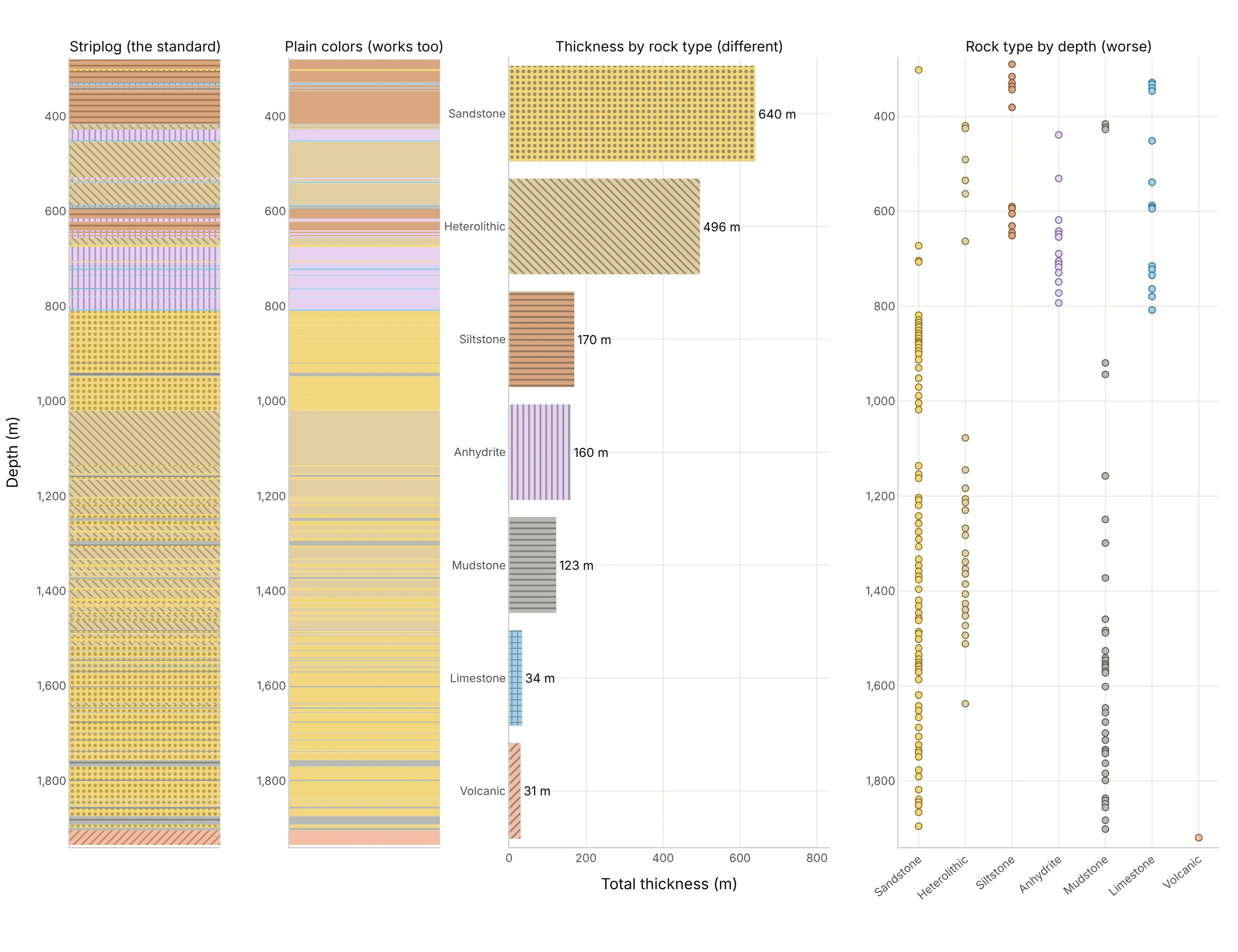
The Kennetcook #2 striplog drawn four ways: the patterned striplog column, the same column in plain colors, horizontal bars of total thickness by rock type from 640 m of sandstone to 31 m of volcanic rock, and a dot plot of each bed’s rock type against depth

Striplog (the standard). The patterns read in black and white and on a phone, and the order of the beds, which carries the geology, is kept.
Plain colors (works too). Colors alone are quicker to draw and fine on screen, but similar colors are hard to tell apart and the convention is lost in print.
Bar chart of thickness by rock type (different). It answers “how much sandstone is there?” (640 m) but throws away where the beds are.
Rock type by depth as dots (worse). It keeps depth but turns thick beds into single dots, so a 26 m anhydrite bed looks the same as a 1 m limestone.

For several wells, a well correlation panel is the striplog’s natural extension, and a 3D view of the wells, like example 4 above, shows how far apart they really are.

How to make a striplog

With AI

ChatGPT, Claude Code, GitHub Copilot, Cursor, and other AI tools are excellent at writing Plotly code. Name Plotly in the prompt, and say how to draw the beds, which fills to use, and how to keep the depth axis shared:

Make a plotly striplog from lith.csv (columns: top_m, base_m, description) and logs.csv (columns: depth_m, gr, rhob).

- make_subplots with 3 columns and shared_yaxes=True, depth increasing downward from 280 to 1,000 m.
- Column 1: one horizontal go.Bar per bed (y = mid-depth, width = base - top, x = 1, base = 0), barmode overlay,
  bargap 0, with marker.pattern fills approximating the FGDC/USGS lithology patterns (dots for sandstone,
  dashes for siltstone and mudstone, + for limestone, | for anhydrite) and a legend.
- Columns 2 and 3: gamma ray (0-200 API) and bulk density (1.95-2.95 g/cm³) as lines, with the scales on top.
- Hover on a bed shows its description, top and base.

With Plotly Studio

Plotly Studio is a desktop app where you point an AI at a dataset and it builds charts and a Dash app around your questions. Ask for a striplog the same way:

Show a striplog of the selected well with a patterned lithology column, gamma ray and density on the same depth axis, and a second view with four wells side by side, their group tops linked between wells, and a dropdown to flatten on any group top.

Make a striplog in Python or JavaScript

This is the code AI tools write under the hood. Plotly has no dedicated striplog trace, so the lithology column is a set of horizontal go.Bar traces, one bar per bed, whose width is the bed’s thickness in depth units, with barmode="overlay" and bargap=0 so the beds touch. The curves are go.Scatter traces on the same depth axis:

import pandas as pd
import plotly.graph_objects as go
from plotly.subplots import make_subplots

beds = pd.read_csv("lith.csv")        # top_m, base_m, description: the Kennetcook #2 striplog
logs = pd.read_csv("logs.csv")        # depth_m, gr, rhob, ...: the same well's wireline logs

# Fills that approximate the FGDC/USGS lithology patterns: (color, pattern shape)
STYLE = {"sandstone": ("#f3d77e", "."), "siltstone": ("#d9a77f", "-"), "mudstone": ("#b9b9b4", "-"),
         "heterolithic": ("#e2cfa0", "\\"), "limestone": ("#9fd0ea", "+"), "anhydrite": ("#e6d2f2", "|"),
         "volcanic": ("#f4bfa6", "/")}
beds["rock"] = [next(k for k in STYLE if k in d.lower()) for d in beds.description]

fig = make_subplots(rows=1, cols=3, shared_yaxes=True, column_widths=[0.3, 0.35, 0.35], horizontal_spacing=0.02)
for rock, b in beds.groupby("rock"):
    color, shape = STYLE[rock]
    fig.add_trace(go.Bar(x=[1] * len(b), y=(b.top_m + b.base_m) / 2, width=b.base_m - b.top_m, orientation="h",
                         name=rock, marker=dict(color=color, pattern=dict(shape=shape, solidity=0.3)),
                         hovertext=b.description), row=1, col=1)
fig.add_trace(go.Scatter(x=logs.gr, y=logs.depth_m, name="GR", line_color="#008300"), row=1, col=2)
fig.add_trace(go.Scatter(x=logs.rhob, y=logs.depth_m, name="RHOB", line_color="#e34948"), row=1, col=3)

fig.update_layout(barmode="overlay", bargap=0, height=900, template="simple_white")
fig.update_yaxes(range=[1000, 280])                                      # depth increases downward
fig.update_yaxes(title_text="Depth (m)", row=1, col=1)
fig.update_xaxes(range=[0, 1], showticklabels=False, row=1, col=1)
fig.update_xaxes(range=[0, 200], title_text="Gamma ray (API)", side="top", row=1, col=2)
fig.update_xaxes(range=[1.95, 2.95], title_text="Density (g/cm³)", side="top", row=1, col=3)
fig.show()

For a fence diagram, give each well its own depth axis (leave out shared_yaxes) and link the same top in neighbouring wells with a multi-axis shape: in plotly.js 3.4 and later (this guide uses plotly.py 7.1), a shape’s xref and yref can be lists, so its first point uses one well’s axes and its second point the other’s. Set dragmode="pan" and drag one well up or down in the browser; the links follow, which is how a geologist slides wells against each other to line up a marker:

import pandas as pd
import plotly.graph_objects as go
from plotly.subplots import make_subplots

d = pd.read_csv("force_wells.csv")    # well, depth_md, group, gr, ...: FORCE 2020 wells
wells = ["15/9-17", "15/9-13"]

# One gamma ray strip per well, each well on its own depth axis (no shared_yaxes)
fig = make_subplots(rows=1, cols=2, horizontal_spacing=0.25, subplot_titles=wells)
tops = []
for i, w in enumerate(wells, start=1):
    g = d[(d.well == w) & d.depth_md.between(2100, 2900)]
    fig.add_trace(go.Scatter(x=g.gr, y=g.depth_md, name=w, line_color="#008300"), row=1, col=i)
    tops.append(g[g.group == "SHETLAND GP."].depth_md.min())          # top of the Shetland Group
fig.update_yaxes(autorange="reversed")
fig.update_xaxes(range=[0, 150], title_text="Gamma ray (API)")

# A multi-axis shape (plotly.js 3.4+): x0/y0 use the first well's axes and x1/y1 the second's,
# so the link between the two Shetland tops follows when either depth axis is panned
fig.add_shape(type="line", xref=["x domain", "x2 domain"], yref=["y", "y2"],
              x0=1, y0=tops[0], x1=0, y1=tops[1], line=dict(color="#2a78d6", width=2, dash="dot"), opacity=1)
fig.update_layout(dragmode="pan", showlegend=False, template="simple_white")
fig.show()

The same multi-axis shapes render in static images too: kaleido 1.5 with plotly.py 7.1 drew every link in this guide’s images.

In JavaScript, plotly.js draws two patterned columns and the links between them like this:

<div id="chart"></div>
<script src="https://cdn.plot.ly/plotly-4.1.1.min.js"></script>
<script>
  // Group intervals (m, measured depth) in two FORCE 2020 wells; Shetland Group is mostly limestone in both
  const wells = {"15/9-17": [2203.1, 2486.1, 2704.1], "15/9-13": [2198.1, 2440.1, 2674.2]};  // Rogaland, Shetland, Cromer Knoll tops
  const traces = [];
  Object.entries(wells).forEach(([name, t], i) => {
    const ax = i === 0 ? "" : "2";
    traces.push(
      {type: "bar", orientation: "h", x: [1], base: 0, y: [(t[0] + t[1]) / 2], width: [t[1] - t[0]], name: "Rogaland Group",
       marker: {color: "#b9b9b4", pattern: {shape: "-", fgcolor: "#55554f", solidity: 0.3}}, xaxis: "x" + ax, yaxis: "y" + ax, showlegend: i === 0},
      {type: "bar", orientation: "h", x: [1], base: 0, y: [(t[1] + t[2]) / 2], width: [t[2] - t[1]], name: "Shetland Group",
       marker: {color: "#9fd0ea", pattern: {shape: "+", fgcolor: "#2f6f93", solidity: 0.3}}, xaxis: "x" + ax, yaxis: "y" + ax, showlegend: i === 0});
  });
  const a = wells["15/9-17"], b = wells["15/9-13"];
  Plotly.newPlot("chart", traces, {
    width: 600, height: 700, barmode: "overlay", bargap: 0, dragmode: "pan",
    xaxis: {domain: [0, 0.3], range: [0, 1], showticklabels: false, title: {text: "15/9-17"}},
    xaxis2: {domain: [0.6, 0.9], range: [0, 1], showticklabels: false, title: {text: "15/9-13"}},
    yaxis: {range: [2750, 2150], title: {text: "Depth (m)"}},
    yaxis2: {range: [2750, 2150], anchor: "x2"},
    // multi-axis shapes: each end on a different well's axes, so the links follow when you pan one well
    shapes: [1, 2].map(k => ({type: "line", xref: ["x domain", "x2 domain"], yref: ["y", "y2"],
                              x0: 1, y0: a[k], x1: 0, y1: b[k], line: {color: "#2a78d6", dash: "dot"}}))
  });
</script>

Share it

Every Plotly chart has a Share chart button (the cloud icon in its toolbar) that uploads it to Plotly Cloud and gives you a link. Only you can see it until you change its visibility.

For a live app, put the chart in a Dash app and publish it with the Plotly Cloud CLI. Coding agents can run these commands for you:

pip install "dash[cloud]"
plotly user login
plotly app publish

If your data has to stay in your own cloud or data center, publish to Dash Enterprise instead.

Dos and don’ts

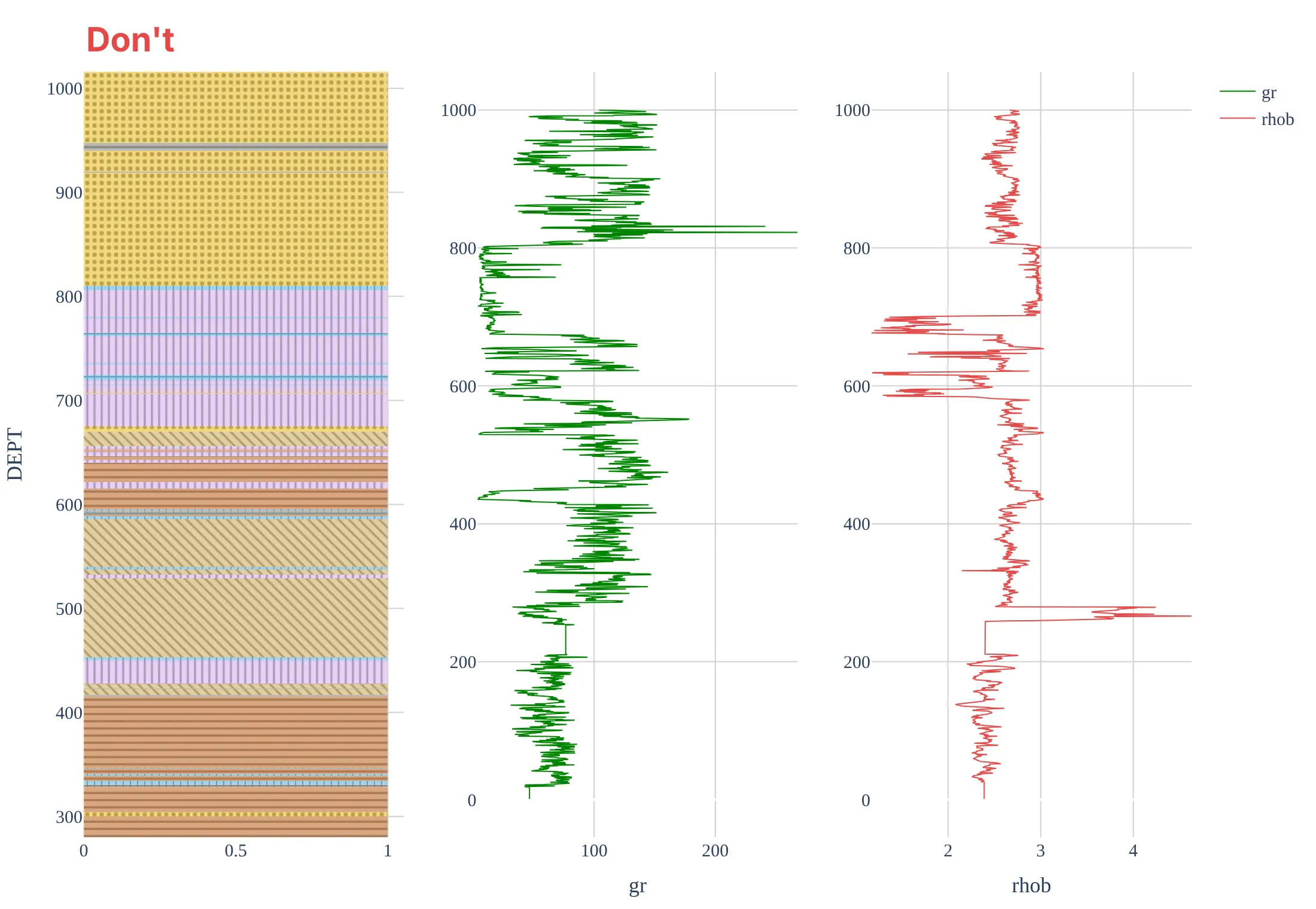
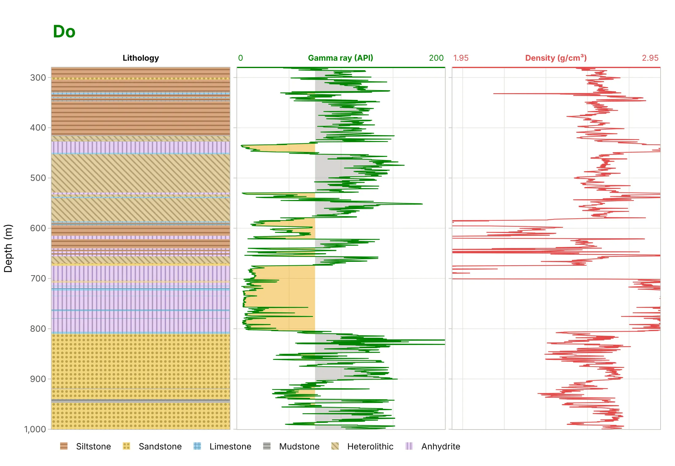
Most striplog mistakes come from treating the lithology column as a separate chart from the logs. Here is the top of the Kennetcook striplog both ways, with the same fills and curve colors.

Don’t let depth increase upward, put the lithology column and each curve on separate, unaligned depth axes, plot the logs above the 280 m casing point (where they read the steel casing, not the rock), leave the fills without a legend, or keep raw mnemonics and a serif font:

A striplog column and two log panels of Kennetcook #2 with depth increasing upward, each panel on its own axis so 1,000 m in the lithology column sits beside different depths in the curves, gamma ray and density running up to 0 m through the casing, no legend for the fills, and a serif font

Do share one depth axis that increases downward, start the logs at the casing point, label each strip’s scale, shade the gamma ray, and add a legend for the rock types:

The same interval, 280 to 1,000 m, as a three-strip composite log with the patterned lithology column, gamma ray with sand and shale shading, and bulk density on one shared downward depth axis, with a legend of six rock types

Checklist

Draw each bed from its top to its base, with no gaps, and use the same fill for the same rock type everywhere.
Follow the FGDC/USGS pattern convention where you can, and show a legend.
Share one depth axis between the lithology and the curves, increasing downward.
In a fence diagram, keep the same strips in the same order for every well, and say how far apart the wells are.
Pair a fence diagram with a map or 3D view of the wells.

Don’t

Flatten on a marker without saying which one, or relabel the depth ticks; keep each well’s true depths.
Mix measured and true vertical depth, or feet and meters, between wells.
Draw a striplog’s beds as dots or lines; their thickness is the information.
Use more fill colors than you have rock types, or patterns no one can tell apart.

Options to customize

A striplog in Plotly is bars, lines, and shapes, so these are the options that matter most. The full lists are in the bar trace reference, the pattern fills page and the shapes documentation.

go.Bar(orientation="h", y=mid, width=thickness, x=1, base=0): one bed as a rectangle from its top to its base.
barmode="overlay", bargap=0: beds that touch, with no gaps between them.
marker.pattern.shape (., -, +, /, \, x, |): the rock type’s fill; fgcolor, size and solidity set the pattern’s color, spacing, and weight.
make_subplots(shared_yaxes=True): lithology and curves on one depth axis; leave it out for a fence diagram with one axis per well.
yaxis.autorange="reversed" or range=[base, top]: depth increasing downward.
Shapes with xref and yref lists (plotly.js 3.4+): lines whose ends sit on different wells’ axes, for correlation links.
"x domain" references: put a link’s ends at the edge of a strip whatever its scale (log or linear).
dragmode="pan" and xaxis.fixedrange=True: drag one well’s depth axis up or down without moving the strips sideways.
hovertemplate with customdata: each bed’s description, top, and base on hover.
go.Scatter3d: the wells’ positions and paths in 3D next to the fence.

More striplog examples

Six more striplogs and composite logs built from real public data, each with its source, the technique that makes it work, and a prompt to rebuild it.

1. Flattening the fence on one marker

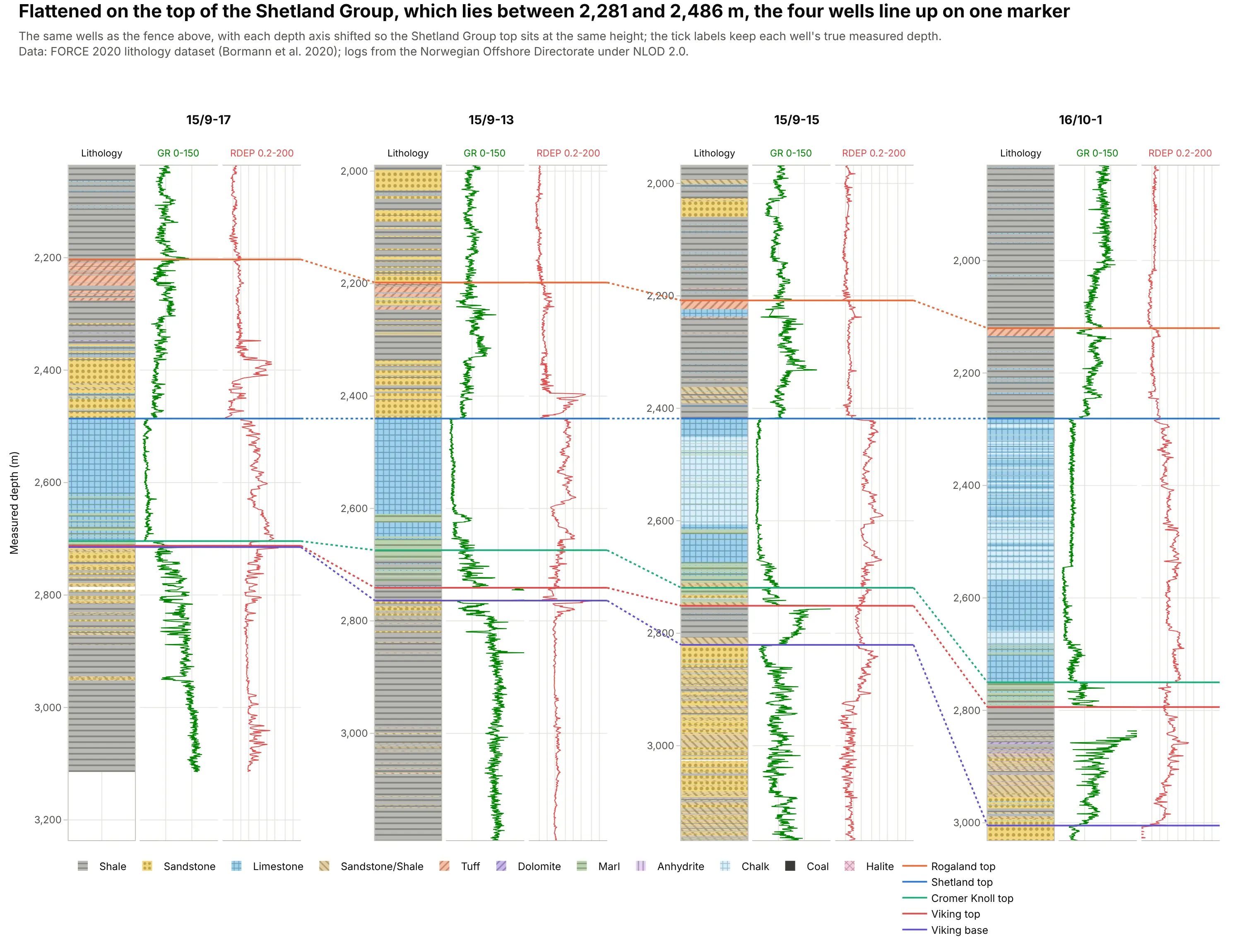
The four-well fence diagram with each well’s depth axis shifted so the top of the Shetland Group lines up at the same height, keeping each well’s true depths in the tick labels, with dotted links to the other group tops above and below

Shifting each well’s depth axis so that the top of the Shetland Group lines up, although it lies between 2,281 and 2,486 m, shows the layers below it rather than the structure: the Shetland Group is 469 m thick in 16/10-1 and 218 m in 15/9-17. In the interactive version, you can drag any well up or down and the links follow. Data: FORCE 2020 lithology dataset (Bormann et al. 2020).

Tip: flatten by changing each depth axis’s range, not the data, so the tick labels keep each well’s true depths.

Get the data from the FORCE 2020 lithology dataset (Bormann et al. 2020, Zenodo and the competition's GitHub
repository, train.csv; columns WELL, DEPTH_MD, GROUP, GR, RDEP, FORCE_2020_LITHOFACIES_LITHOLOGY) for wells 15/9-17,
15/9-13, 15/9-15 and 16/10-1.

Build a plotly fence diagram: three strips per well (lithology bars with pattern fills, gamma ray, deep resistivity on
a log scale), one depth axis per well with its range shifted so the top of SHETLAND GP. lines up, and multi-axis
shape links (xref and yref lists) between the same group tops in neighbouring wells.

2. A composite log close up: anhydrite in Kennetcook #2

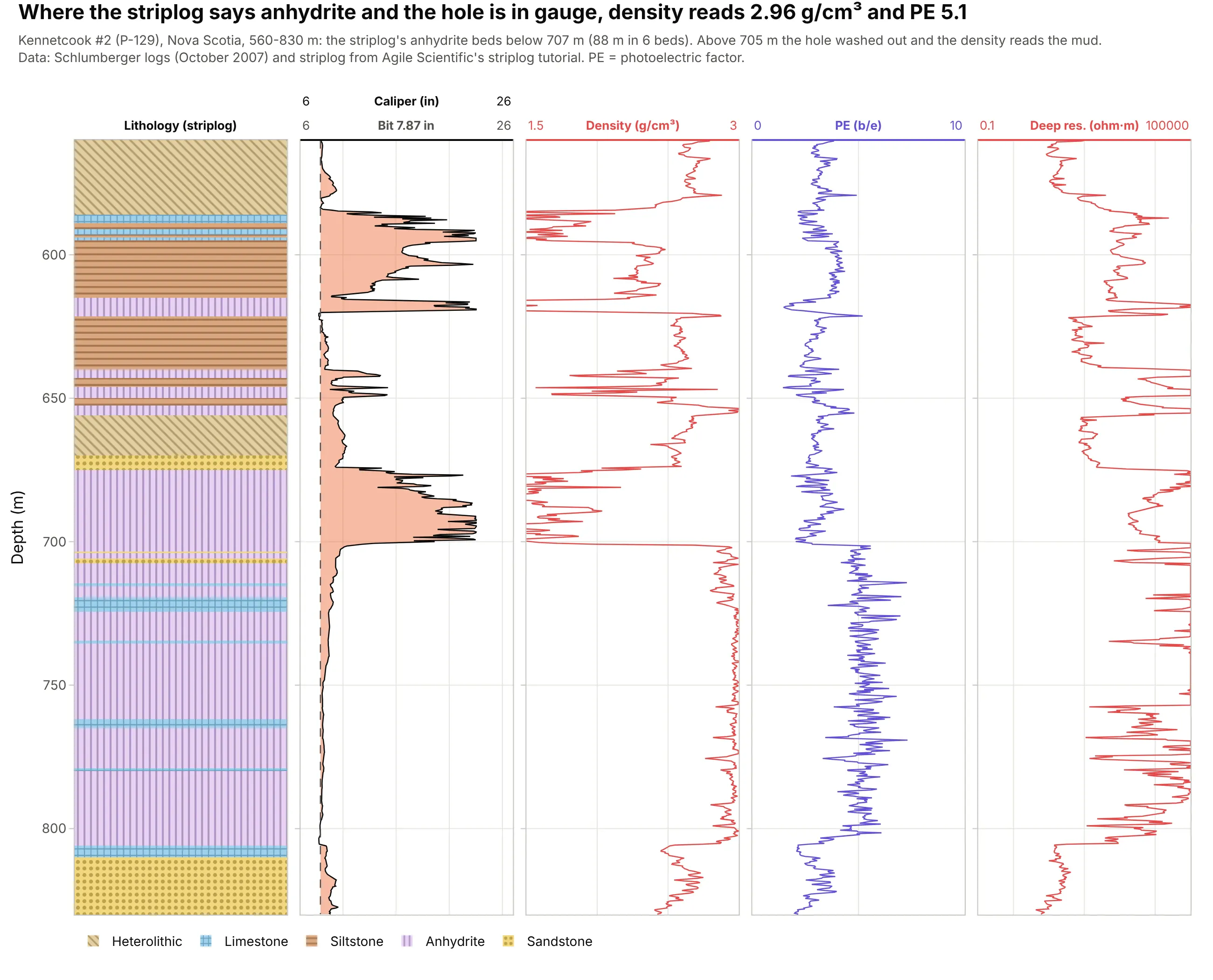
A five-strip composite log of Kennetcook #2 from 560 to 830 m: the lithology column with siltstone, limestone, heterolithic rock, and long lilac anhydrite beds, a caliper that balloons to over 20 inches above 705 m, density that drops to mud values in the washouts and reads near 2.96 g/cm³ in the anhydrite below, photoelectric factor near 5, and resistivity at the tool’s ceiling

Below 707 m, the striplog’s six anhydrite beds (88 m in all) read a median density of 2.96 g/cm³ and a PE of 5.1 on the logs, so the description and the measurements agree. Above 705 m the hole washed out, and the density log reads the drilling mud instead. Data: Kennetcook #2 (P-129) via Agile Scientific.

Tip: put the caliper next to the lithology, so readers know where the logs can’t be trusted.

Get the data from Agile Scientific's striplog tutorial (P-129_out.LAS and P-129_striplog_from_image.las, Kennetcook #2,
Nova Scotia; curves CALI, RHOB, PEF, RLA5 and intervals top, base, description) for 560-830 m.

Build a plotly composite log: a patterned lithology column, caliper with the 7.87 in bit size and washouts shaded,
density, photoelectric factor and deep resistivity on a log scale, all on one depth axis.

3. Chalk, shale and sandstone in well 15/9-15

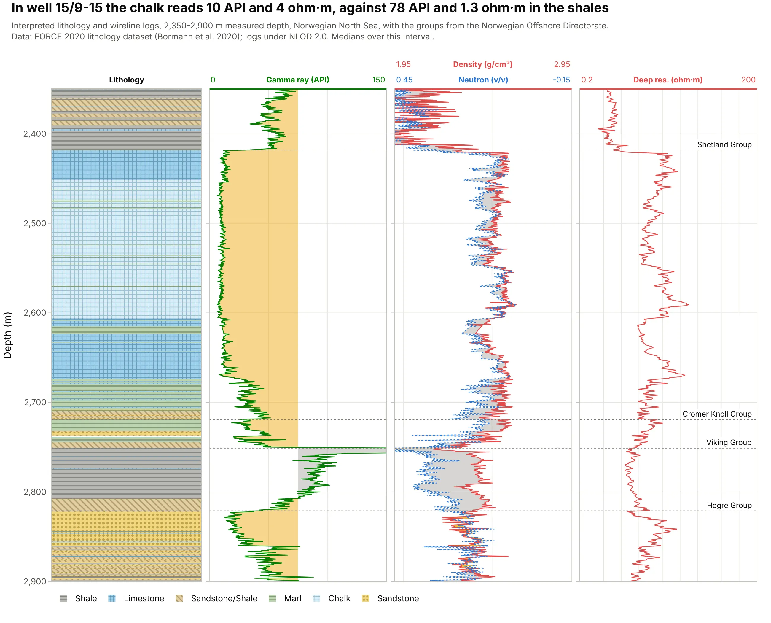
A four-strip composite log of well 15/9-15 from 2,350 to 2,900 m: lithology with blue chalk and limestone, gray shale, and yellow sandstone, gamma ray reading low in the chalk, the neutron-density overlay, and deep resistivity, with the Shetland, Cromer Knoll, Viking, and Hegre group tops

In well 15/9-15 the interpreted chalk reads a median of 10 API and 4 ohm·m, against 78 API and 1.3 ohm·m in the shales, which is why the lithology labels and the logs line up so cleanly at the top of the Shetland Group. Data: FORCE 2020 lithology dataset (Bormann et al. 2020).

Tip: label the group tops on the right edge of the last strip, so the lithology column stays clear.

Get the data from the FORCE 2020 lithology dataset (train.csv) for well 15/9-15, 2,350-2,900 m (columns DEPTH_MD,
GROUP, GR, RHOB, NPHI, RDEP, FORCE_2020_LITHOFACIES_LITHOLOGY with the competition's lithology key).

Build a plotly composite log: a patterned lithology column, gamma ray shaded at 75 API, density with neutron on the
standard overlay, deep resistivity on a log scale, and the group tops as dotted lines with labels.

4. A lithology column from a geology report: Utah FORGE

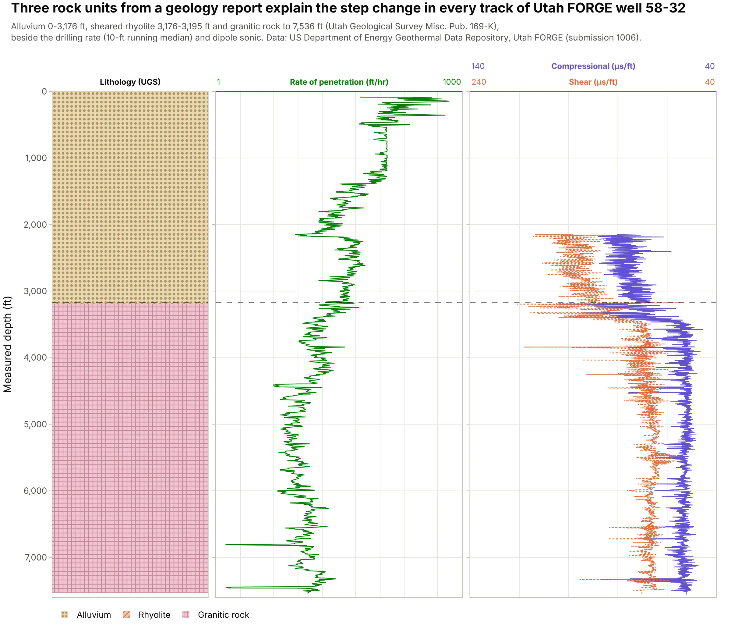
A three-strip log of Utah FORGE geothermal well 58-32 from 0 to 7,600 ft: a lithology column with dotted alluvium down to 3,176 ft and pink granitic rock below, rate of penetration on a log scale dropping at the contact, and compressional and shear sonic slowness that fall sharply into the granite

A striplog can be as short as three units from a report: alluvium to 3,176 ft, a 19 ft sheared rhyolite, and granitic rock to 7,536 ft, where the drilling rate falls and sound travels faster. The well is the research site of Utah FORGE (the Frontier Observatory for Research in Geothermal Energy). Data: US Department of Energy Geothermal Data Repository; lithology from Utah Geological Survey Misc. Pub. 169-K.

Tip: a lithology column with few, long units still earns its place, because it explains every step in the curves.

Get the data from the US Department of Energy Geothermal Data Repository, Utah FORGE well 58-32 (submission 1006:
the DSI sonic LAS with DTCO and DTSM, and the one-foot drilling CSV with Depth and ROP(1 ft)), and the lithology from
Utah Geological Survey Misc. Pub. 169-K (alluvium 0-3,176 ft, rhyolite 3,176-3,195 ft, plutonic rock below).

Build a plotly composite log in feet: a patterned lithology column (dots for alluvium, + for granite), the drilling
rate on a log scale and compressional and shear slowness.

5. A grain-size striplog

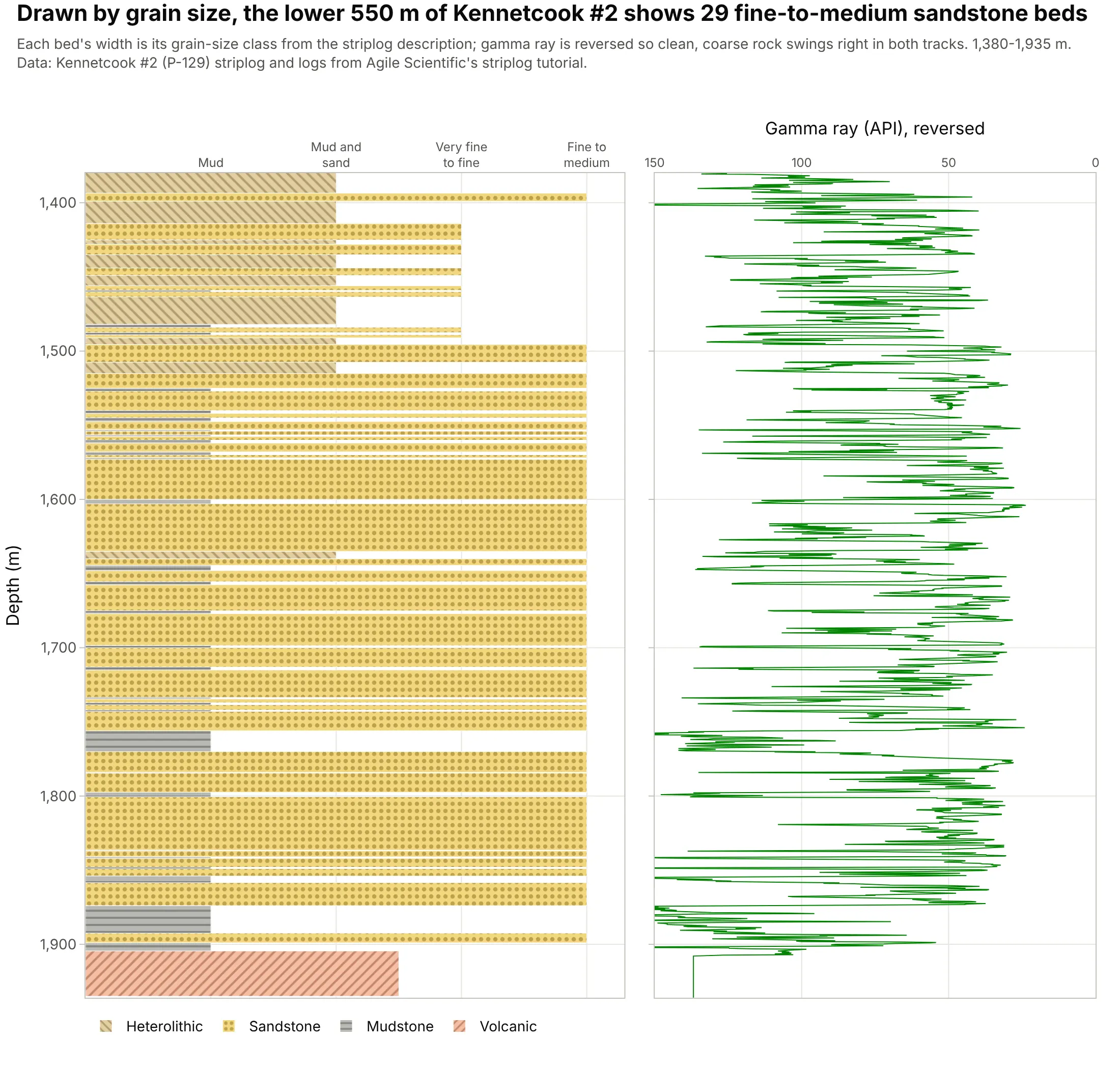
Lower 550 m of Kennetcook #2 drawn as a grain-size striplog: each bed is a bar whose length is its grain-size class, from mud to fine-to-medium sand, with yellow dotted sandstones reaching furthest right and gray mudstones shortest, next to a reversed gamma ray curve that swings right in the sandstones

Drawing each bed as wide as its grain size, the traditional way to draw a core description, shows 29 fine-to-medium sandstone beds in the lower 550 m of Kennetcook #2, and the reversed gamma ray beside it swings the same way. Data: Kennetcook #2 (P-129) via Agile Scientific.

Tip: set each bar’s length to the grain-size class and keep the fill for the rock type, so one column carries both.

Get the data from Agile Scientific's striplog tutorial (P-129_striplog_from_image.las: top, base, description such as
"Grey, sandstone, f-m") and P-129_out.LAS (GR) for 1,380-1,935 m.

Build a plotly grain-size striplog: one horizontal bar per bed with length 1 (mud) to 4 (fine to medium sand) and a
lithology pattern fill, next to gamma ray on a reversed 150-0 API scale, sharing depth.

6. A formation column next to the logs

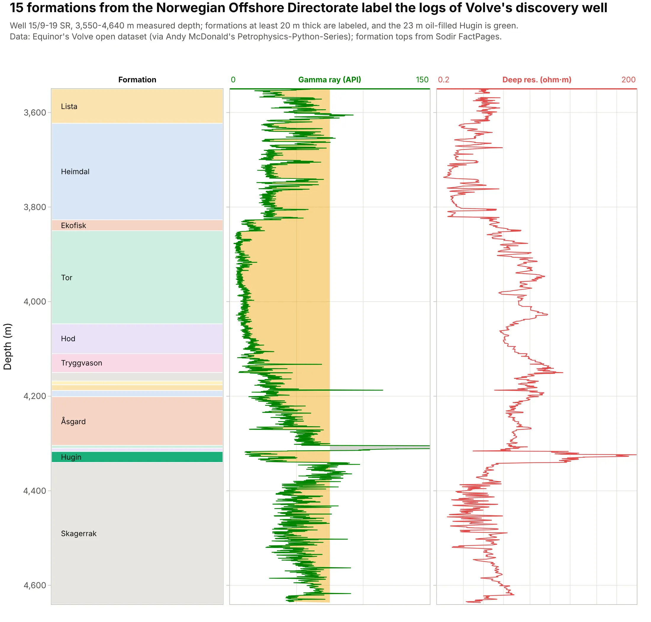
A three-strip log of Volve discovery well 15/9-19 SR from 3,550 to 4,640 m: a column of 15 formations in pastel colors with the oil-bearing Hugin in green, gamma ray with sand shading, and deep resistivity on a log scale

The striplog column doesn’t have to be lithology: here it holds the 15 formations the Norwegian Offshore Directorate picked in Volve’s discovery well, so every log response has a name, including the 23 m oil-filled Hugin. Data: Equinor’s Volve open dataset (via Andy McDonald’s Petrophysics-Python-Series); tops from Sodir FactPages.

Tip: label only the intervals tall enough to hold text, and let hover name the thin ones.

Get the data from Equinor's Volve open dataset (15-9-19_SR_COMP.LAS, curves GR and RDEP) and the formation tops of
wellbore 15/9-19 SR from the Norwegian Offshore Directorate's FactPages (columns: top, base, formation), 3,550-4,640 m.

Build a plotly composite log: a formation column as horizontal bars with names, the Hugin Formation highlighted,
gamma ray shaded at 75 API and deep resistivity on a log scale.