
Chris Parmer
November 15, 2026
Skew-T Log-P Diagrams - A Complete Guide
TL;DR
- A skew-T log-P diagram (skew-T for short) is the standard chart for an atmospheric sounding, the temperature, dew point and wind that a weather balloon measures on its way up: air pressure in hectopascals (hPa) runs up the y axis on a log scale with 1,000 hPa (close to sea level) at the bottom, and temperature runs along an x axis whose lines of constant temperature (isotherms) are skewed 45 degrees to the right.
- Skew-T diagrams are one of four commonly used thermodynamic diagrams, with the emagram, the Stüve diagram and the tephigram, and the chart is similar to a psychrometric chart in that it draws the physics of moist air as a grid behind your measurements.
- Forecasters read it to judge thunderstorm potential from a parcel's convective available potential energy (CAPE), pilots to find cloud bases, freezing levels and the jet stream, and glider pilots to forecast the height of thermals.
- You can make a skew-T with Plotly from go.Scatter lines, using the MetPy package for the physics (adiabats, parcel path, CAPE) and Plotly for the drawing. The code is below, together with ten examples on real soundings.
What is a skew-T log-P diagram?
Skew-T log-P diagrams look like this:
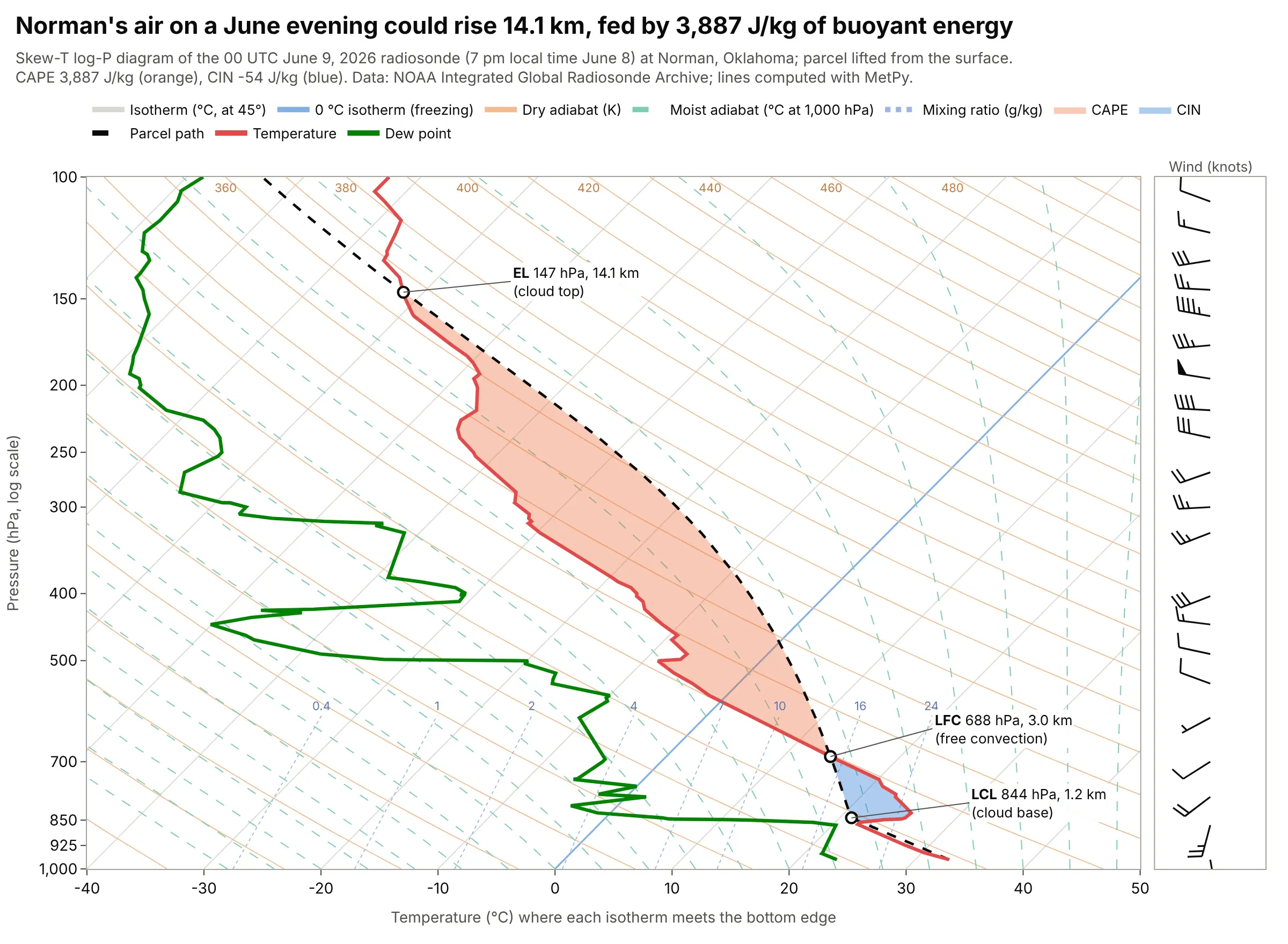
Data: a radiosonde (a weather balloon carrying a small sensor package) launched at Norman, Oklahoma at 00 coordinated universal time (UTC) on June 9, 2026, which was 7 pm local time on June 8, from the Integrated Global Radiosonde Archive (IGRA) of NOAA (the National Oceanic and Atmospheric Administration); lines computed with MetPy.
How do you read a skew-T log-P diagram? In the example above, notice these things:
- The red line is the temperature the balloon measured at each pressure, and the green line is the dew point, the temperature at which the air would become saturated. At the surface (970 hPa) they were 32.9 and 23.3 °C, and at 700 hPa they were 15.4 and -5.0 °C, so the air aloft was much drier: the gap between the lines, the dew point depression, grew from 9.6 to 20.4 °C. Where the two lines touch, the air is saturated and a cloud is likely.
- Pressure falls as the balloon rises, so the top of the chart is high up: 500 hPa was at 5.9 km above sea level in this sounding, 200 hPa at 12.5 km and 100 hPa at 16.7 km. The axis is logarithmic because pressure falls roughly by the same fraction for each equal step up, which spaces the heights more evenly than a linear axis would.
- The dashed black line is the path of a parcel of air lifted from the surface. It cools along a dry adiabat until it reaches the lifting condensation level (LCL) at 844 hPa, 1.2 km above the ground, where a cloud would form. Above that it is cooler than its surroundings until the level of free convection (LFC) at 688 hPa (3.0 km), and warmer than its surroundings from there up to the equilibrium level (EL) at 147 hPa (14.1 km), the likely top of a storm cloud.
- The orange area is the CAPE, 3,887 joules per kilogram (J/kg), the energy the parcel gains from being warmer than the air around it. The blue area is the convective inhibition (CIN), -54 J/kg, the energy the parcel has to be given to get from the surface to the LFC.
- The wind barbs on the right show that the wind at the surface came from 170 degrees (south-southeast) at 10 knots and turned clockwise with height to 279 degrees (west) at 56 knots at 200 hPa. The filled triangle and half feather at 200 hPa mean 55 knots.
It's often used for charts like these:
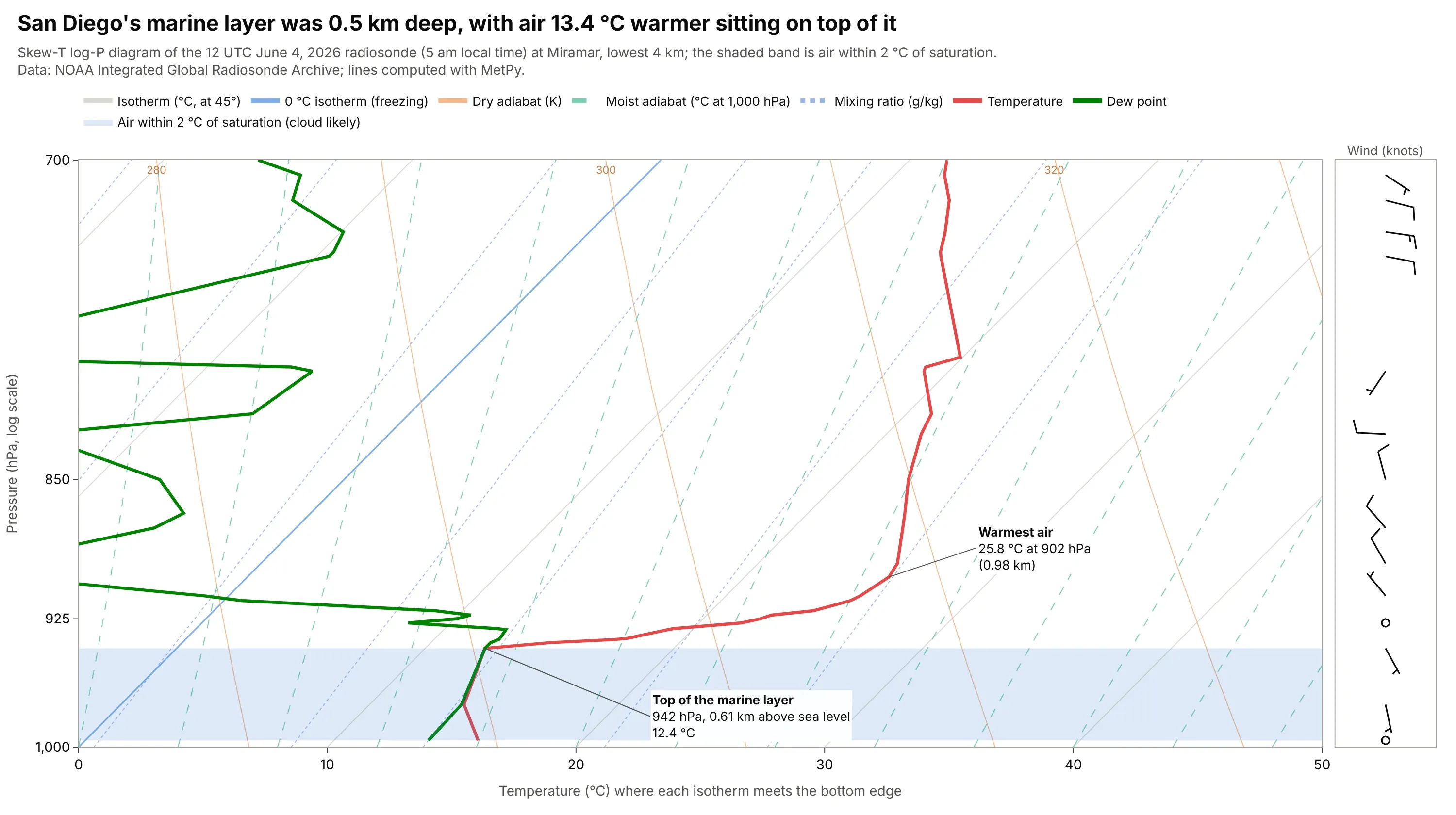
Low cloud and aviation ceilings. A temperature that rises with height (an inversion) shows as the red line swinging right, and the dew point touching it marks the saturated layer where low cloud sits. At San Diego's Miramar station the marine layer was 0.5 km deep with air 13.4 °C warmer on top of it, which caps the cool layer below it and keeps any cloud in that layer from rising. Data: NOAA IGRA, Miramar (station USM00072293), 12 UTC June 4, 2026.
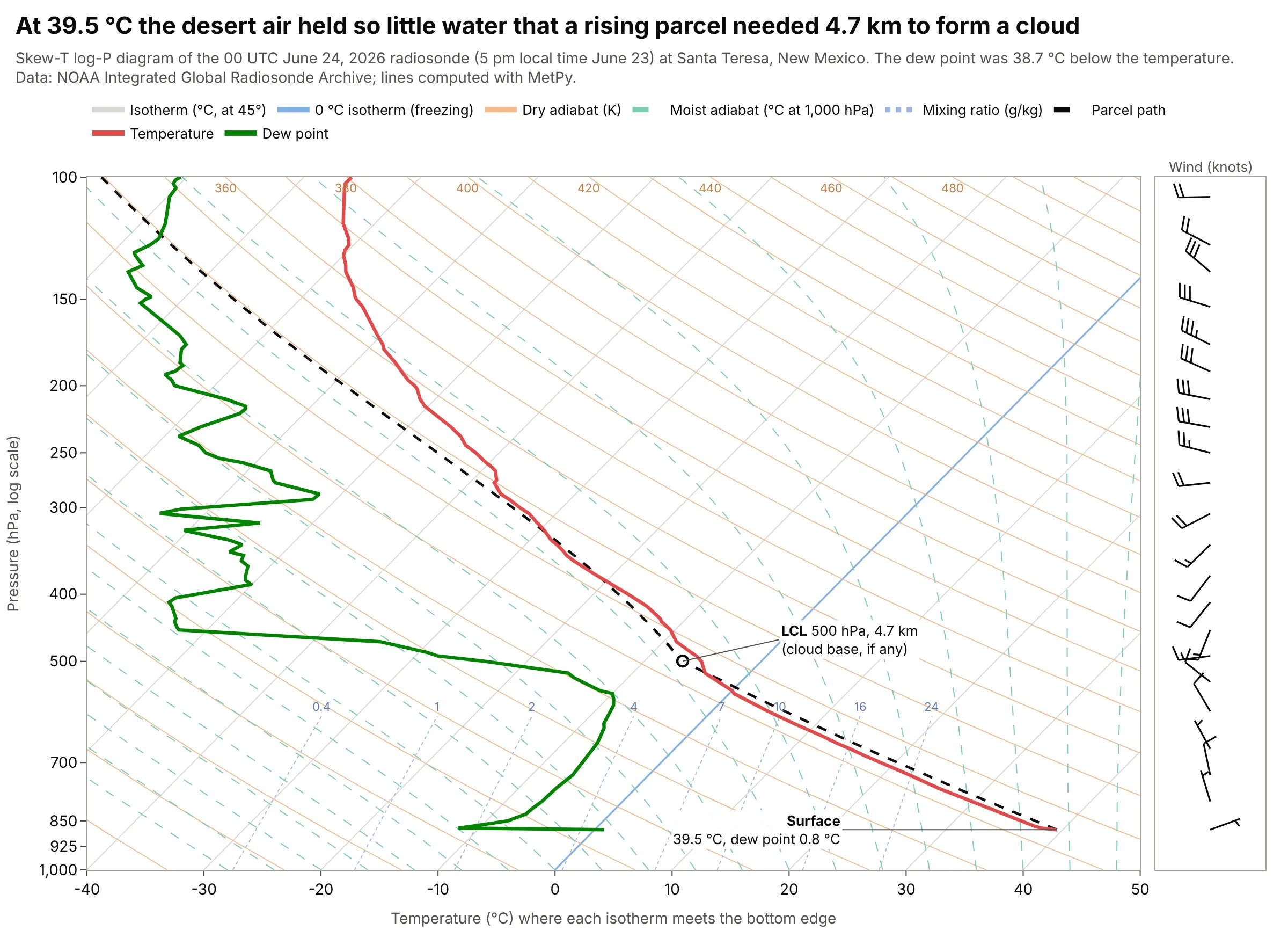
Dry air and cloud base. The gap between the red and green lines is the dew point depression, so a dry atmosphere shows as a wide gap, and a temperature that follows a dry adiabat means the air is well mixed. At Santa Teresa, New Mexico, the surface air was 39.5 °C with a dew point of 0.8 °C, so a rising parcel would not reach its LCL until 500 hPa, 4.7 km above the ground. Data: NOAA IGRA, Santa Teresa (station USM00072364), 00 UTC June 24, 2026.
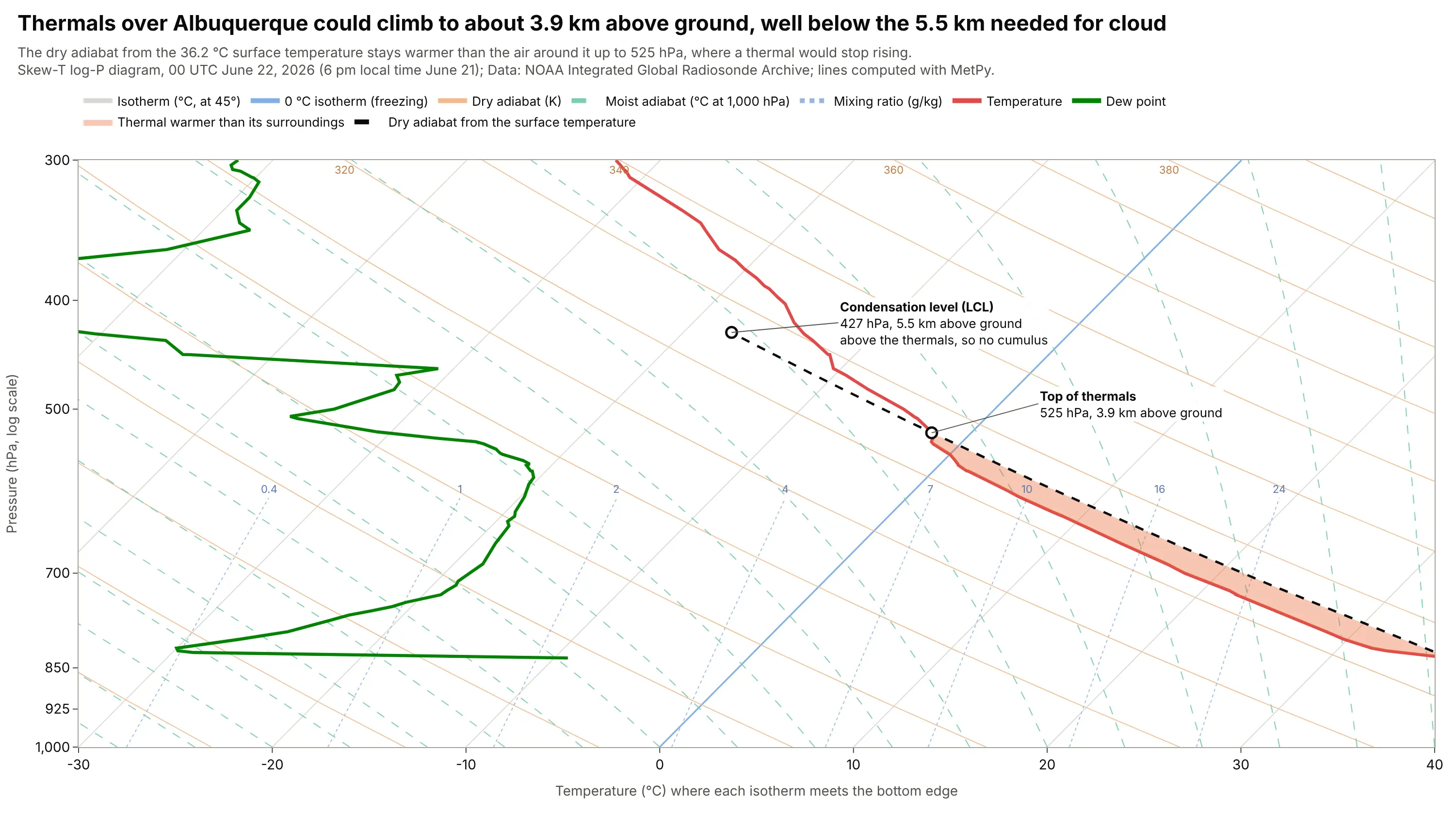
Gliding. Glider pilots use the chart to forecast the strength of thermals and the height of the cloud base (Wikipedia says the diagrams are widely used for this): a thermal rises along a dry adiabat until the air around it is as warm. Over Albuquerque the dry adiabat from the 36.2 °C surface stays warmer than the air up to 525 hPa, 3.9 km above ground, well below the 5.5 km needed for cloud, so no cumulus would have marked the thermals. Data: NOAA IGRA, Albuquerque (station USM00072365), 00 UTC June 22, 2026.
How to read a skew-T log-P diagram
A skew-T draws five things on one grid: two lines you measured (temperature and dew point), four families of lines that are pure physics (isotherms, dry adiabats, moist adiabats and mixing ratio lines), and the wind. Once you know what each line family is for, the chart answers most questions about the atmosphere above one place. This is the same sounding as above with every family labeled once:
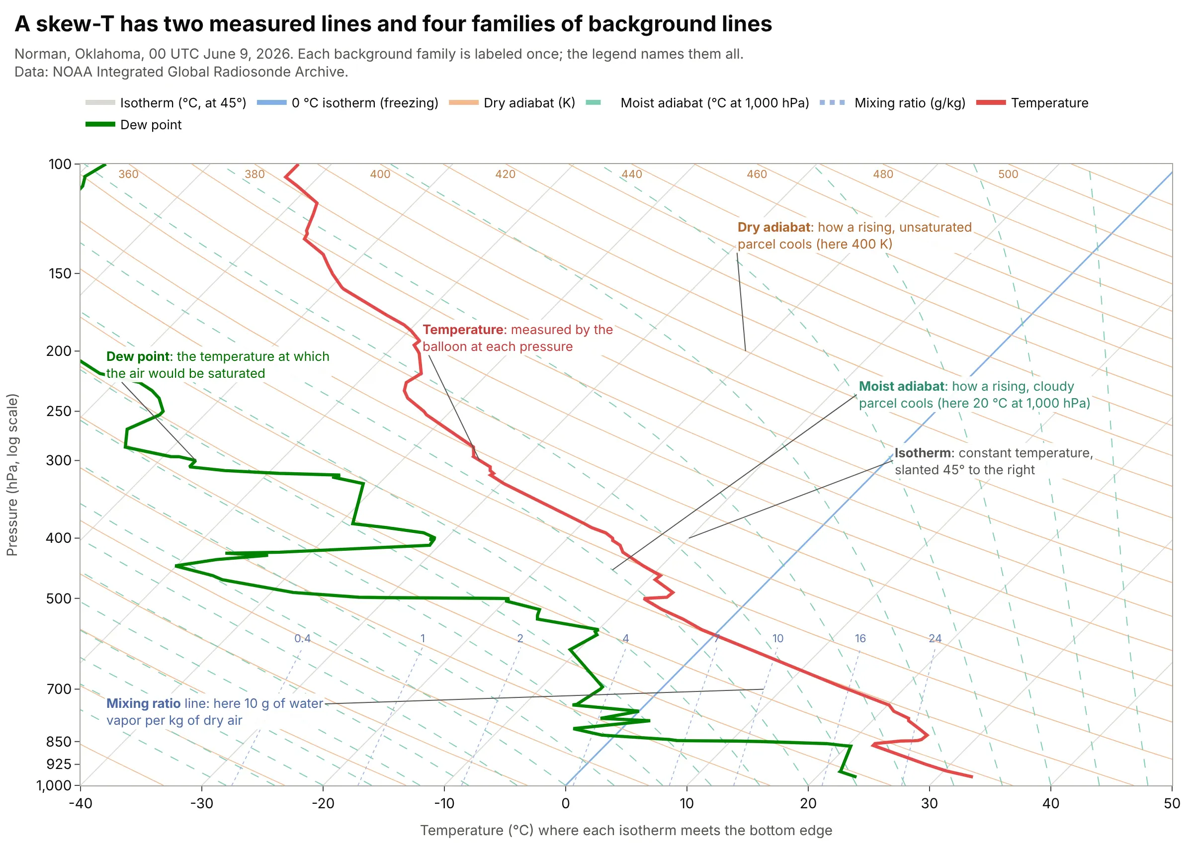
Data: NOAA IGRA, Norman, Oklahoma (station USM00072357), 00 UTC June 9, 2026; background lines computed with MetPy.
A sounding is a column of air measured on the way up
A radiosonde is a weather balloon carrying sensors for pressure, temperature, humidity and (by tracking its position) wind, and it keeps reporting as it rises to 30 km or more. The data is one vertical profile, called a sounding, so the chart shows how the atmosphere is built above one place at one time. The sounding in this guide has 164 reported levels from 970 down to 10 hPa. Norman's archive for 2026 (through November 14) holds 316 soundings at 00 UTC, 314 at 12 UTC and 37 at other hours, mostly extra launches in the afternoon. The heights quoted in this guide are geopotential heights, in meters above sea level unless the text says above ground.
The pressure axis (log P)
Pressure is the vertical axis because a balloon measures it directly and because a given pressure level is more meaningful for weather than a height. In the nine soundings used here, 850 hPa was 1.46 to 1.55 km above sea level, 700 hPa was 3.0 to 3.2 km, 500 hPa was 5.6 to 6.0 km, 300 hPa was 9.2 to 9.8 km, 200 hPa was 11.8 to 12.6 km and 100 hPa was 16.1 to 16.8 km. The standard levels (1,000, 850, 700, 500, 300, 200 and 100 hPa) are the ones forecasters talk about, so they are the labeled ticks.
The temperature axis, and why it is skewed
The x axis is temperature in degrees Celsius, and the lines of constant temperature (isotherms) run up and to the right at 45 degrees, which gives the diagram its name. To read a temperature, follow the isotherm down to the bottom edge, where the tick labels are; reading straight down from a point on the chart gives the wrong value, which is the most common mistake with skew-T diagrams. The skew is there because the air gets colder with height: on a plot with upright isotherms (an emagram), the temperature line would run off the left edge, but the skew keeps most soundings near the middle of the chart. It also opens the angle between isotherms and dry adiabats, as the history section shows.
The temperature and dew point lines
The red line is the temperature the air actually had at each pressure, and the green line is the dew point, the temperature to which the air would have to cool, at the same pressure and without gaining or losing water, to become saturated. A dew point equal to the temperature means 100% relative humidity. Because the dew point can never be higher than the temperature, the green line stays to the left of the red line, and the distance between them tells you how dry the air is. The psychrometric chart guide explains dew point, wet bulb and relative humidity at the surface in more depth, since it is the same physics drawn for air near the ground.
Dry adiabats (orange)
A parcel of air that rises into lower pressure expands and cools, and if no water condenses it cools at the dry adiabatic lapse rate, which is gravity divided by the specific heat of air at constant pressure, about 9.8 °C per kilometer (MetPy's dry_lapse computes it). The dry adiabats are the lines that parcel follows, and each one is labeled by its potential temperature in kelvin (K), the temperature the parcel would have if it were brought down to 1,000 hPa. In a well-mixed layer, such as the desert sounding above, the red line runs parallel to the dry adiabats.
Moist adiabats (green dashes)
Once a rising parcel is saturated, condensing water releases heat, so it cools more slowly than the dry rate and its path bends away from the dry adiabats. These curved lines are the moist adiabats, labeled here by the temperature they have at 1,000 hPa, and a cloudy parcel follows them. In the main example the parcel switches from a dry to a moist adiabat at the LCL.
Mixing ratio lines (dotted)
The mixing ratio is the mass of water vapor per kilogram of dry air, in grams per kilogram (g/kg), and the dotted lines mark constant values from 0.4 to 24 g/kg in the lower atmosphere. If you find where the dew point sits relative to these lines, you can read how much water the air holds: the surface air at Norman held 18.9 g/kg. A rising parcel keeps its mixing ratio until it condenses, so its dew point follows one of these lines up to the LCL.
Wind barbs
Plotly has no wind barb trace, so the guide draws them as lines in a second panel. Each barb is a staff that points toward the direction the wind comes from, with feathers on its clockwise side in the northern hemisphere. A half feather is 5 knots, a full feather 10 knots and a filled triangle 50 knots, as the station model on Wikipedia describes.
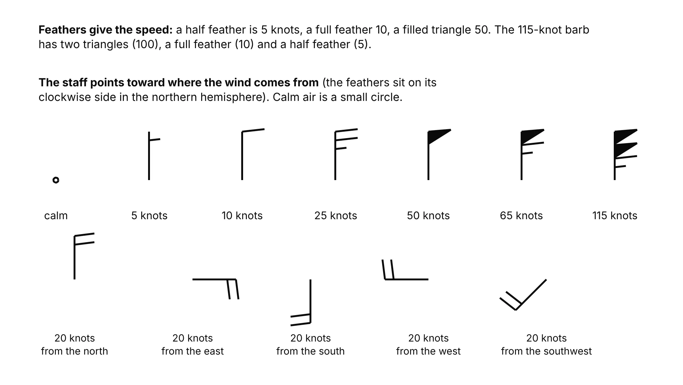
A turning wind (a wind that changes direction with height) is one of the things a skew-T shows quickly. In the Norman example the wind turned clockwise from south-southeast at the surface to west at 200 hPa, going through 205 degrees at 28.8 knots at 850 hPa and 258 degrees at 5.8 knots at 500 hPa.
Lifting a parcel: LCL, LFC, EL, CAPE and CIN
The best-known use of the chart is to lift an imaginary parcel of air from the surface and see what it does. The parcel rises along a dry adiabat, its dew point follows a mixing ratio line, and the two meet at the LCL, where it becomes saturated and a cloud base forms. Above the LCL it follows a moist adiabat. Wherever the parcel is warmer than the surrounding air it is buoyant and keeps rising, and the energy it gains in that layer is the CAPE. Wherever it is cooler it needs a push, and the energy of that push is the CIN. The LFC is where the parcel first becomes warmer than its surroundings, and the EL is where it stops being warmer.
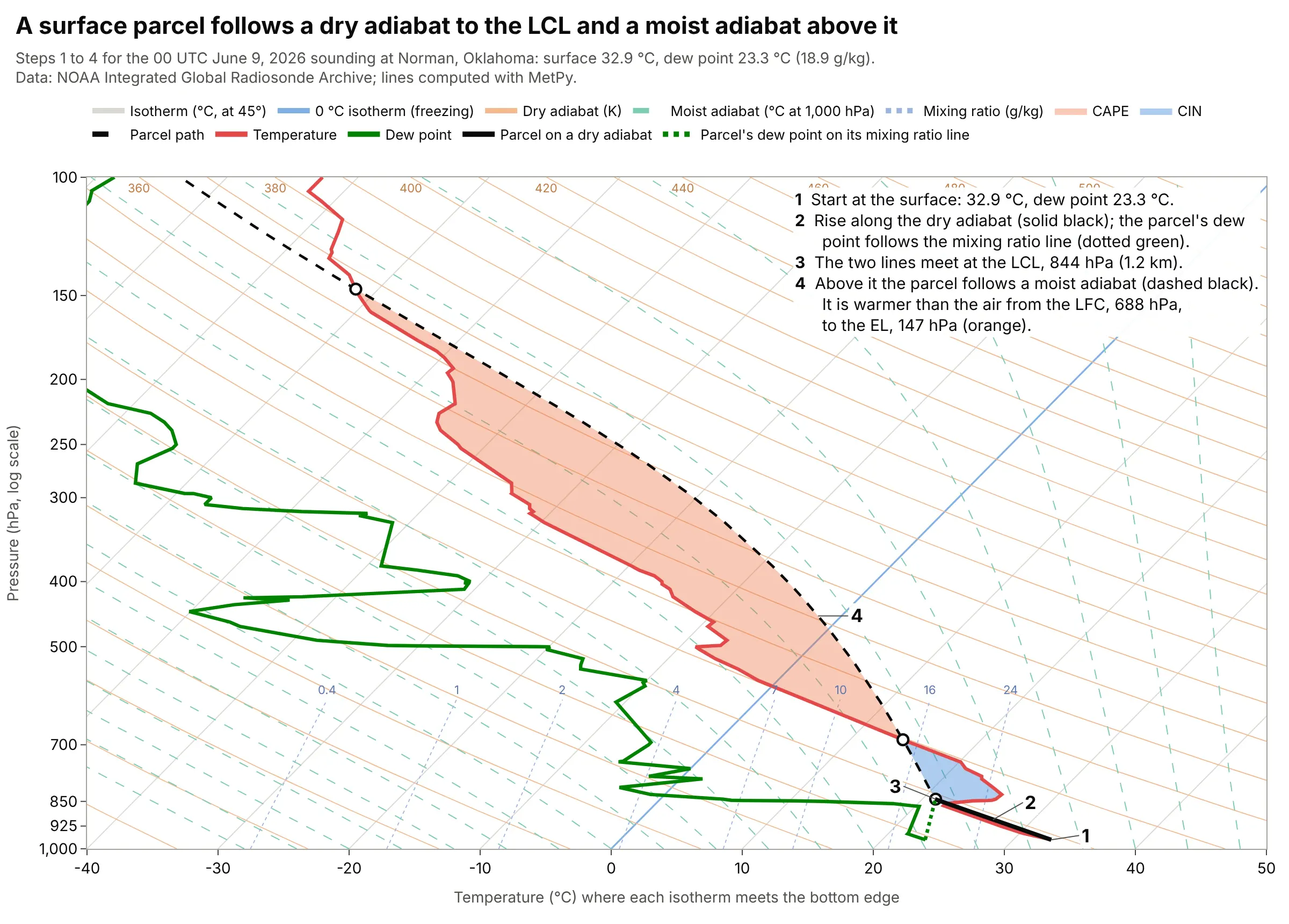
Data: NOAA IGRA, Norman, Oklahoma, 00 UTC June 9, 2026; parcel computed with MetPy (parcel_profile, cape_cin, lcl, lfc, el) without the virtual temperature correction.
MetPy integrates CAPE and CIN from the sounding rather than measuring the shaded area on the screen. The example below shows that the answer depends on which parcel you lift.
Who uses the chart, and for what decisions
Forecasters use skew-T diagrams to judge whether air will form storms and how strong they could be, from the CAPE, the CIN and the wind profile. Pilots use them to find cloud bases and layers, the freezing level, where clouds are below freezing, and the height of the jet stream and the tropopause. Glider pilots use them for thermals, and atmospheric scientists and students use them to learn how the atmosphere is stratified. Chris Parmer's compendium of canonical charts lists the skew-T log-P under aviation and meteorology.
Units and conventions
Pressure is in hPa (the same number as millibars), temperature in degrees Celsius, wind speed in knots and heights in meters or kilometers above sea level. Pressure has 1,000 hPa at the bottom and runs to 100 hPa (or higher) at the top. Different countries favor different diagrams: the emagram is used primarily in European countries and the tephigram primarily in the United Kingdom and Canada (Wikipedia: emagram and tephigram).
A short history
The first atmospheric thermodynamic diagram was the emagram, devised in 1884 by Heinrich Hertz according to Wikipedia; Napier Shaw followed with the tephigram in 1915 (Wikipedia), and the Stüve diagram became the fourth member of the family. In 1947 Nicolai Herlofson proposed a modification to the emagram that keeps the isobars straight and horizontal but skews the isotherms, giving a large angle between isotherms and dry adiabats like the one in the tephigram, which made it useful for the analysis methods the United States Air Force was adopting (Wikipedia). We could not find Herlofson's original paper online, so this is a redraw of his idea, not of his chart: the same Norman sounding on an emagram and on a skew-T, with the angle between an isotherm and a dry adiabat at 500 hPa measured on the screen.
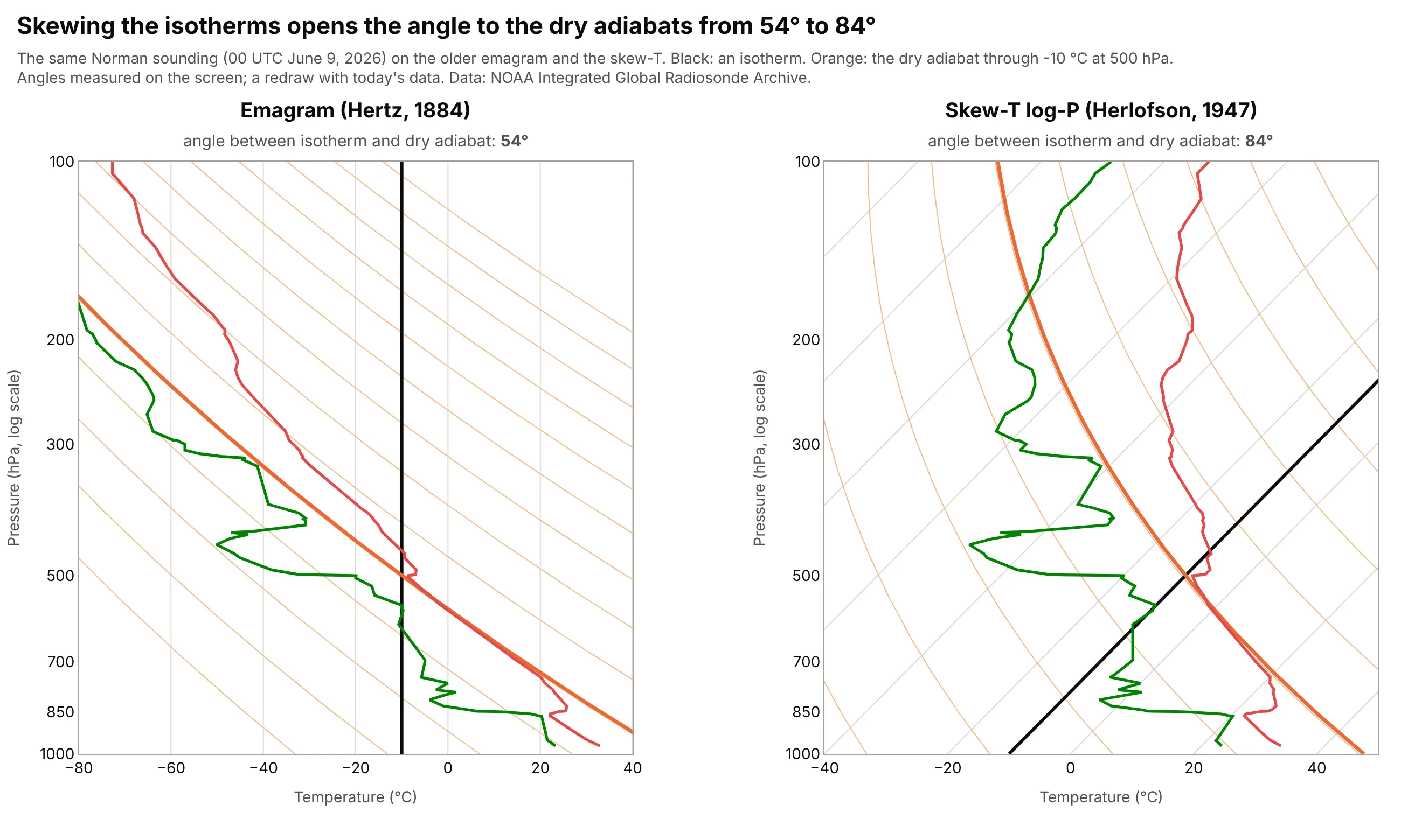
Data: NOAA IGRA, Norman, Oklahoma, 00 UTC June 9, 2026; both panels drawn with Plotly from the same temperature, dew point and the isotherm and dry adiabat through -10 °C at 500 hPa.
Alternatives to a skew-T log-P diagram
Here's the same Norman sounding drawn six ways. Some are better for the question, some worse, some just different:
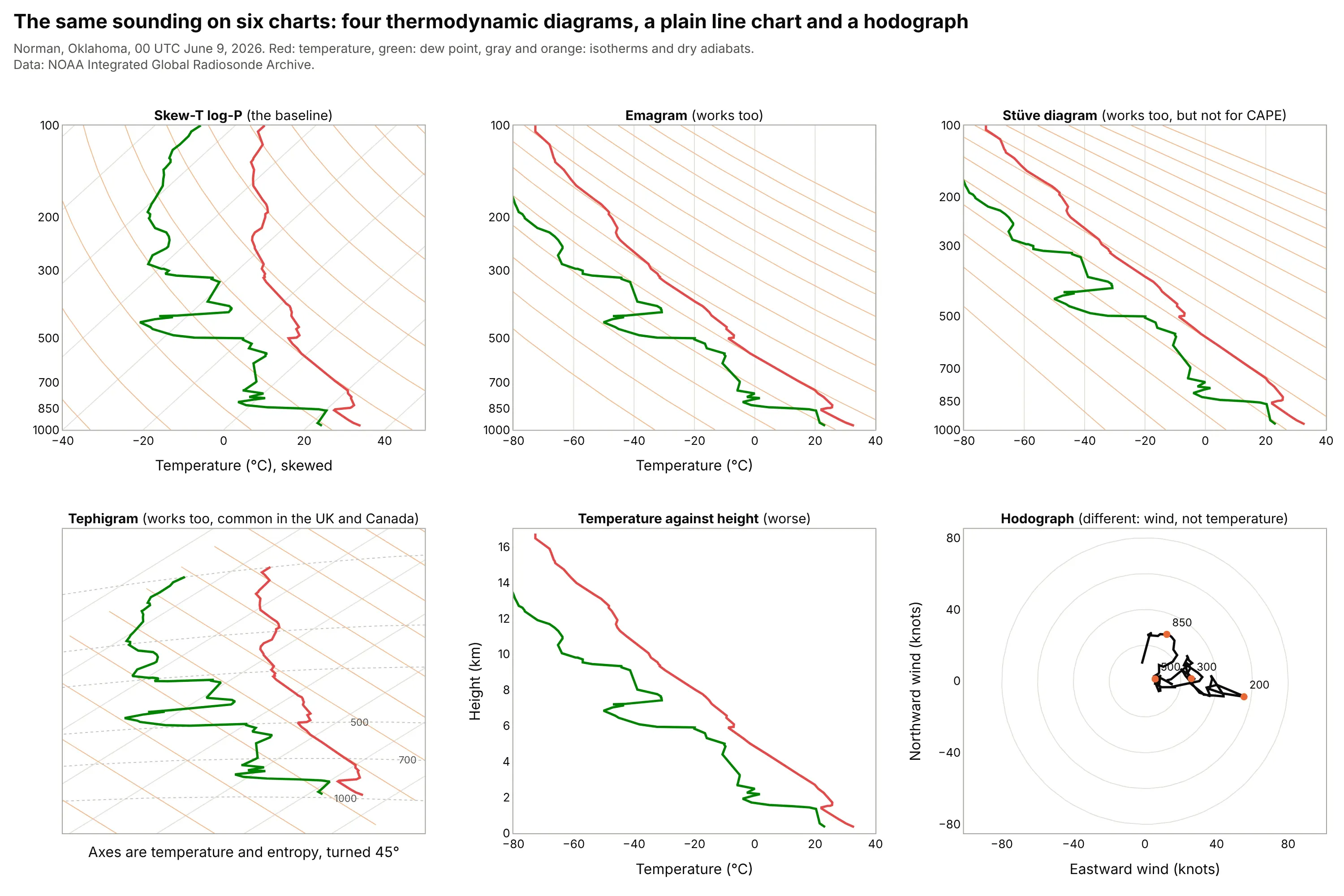
- Emagram (works too). Temperature on a straight x axis and log pressure up, as in the oldest diagram; the dry adiabats cross the isotherms at a smaller angle (54 degrees against 84 in the history figure) and the temperature line runs off to the left, but it reads the same way.
- Stüve diagram (works too, but not for CAPE). Pressure to the power 0.286 on the y axis makes dry adiabats straight lines, which is handy for teaching, but it does not preserve the area-energy relationship, so Wikipedia says it cannot be used to calculate CAPE.
- Tephigram (works too). Temperature and entropy axes turned 45 degrees, with areas that correspond to equal energies, which is why the British Met Office and the Canadian weather service use it (Wikipedia); the isobars are curved, so it takes some getting used to.
- Temperature against height (worse). A line chart of temperature and dew point against height is easy to read, but it has no adiabats, so you cannot lift a parcel or find the LCL, and the parcel's CAPE is not visible.
- Hodograph (different). A hodograph plots the wind's eastward and northward components at each level, so it shows wind shear better than barbs, but it has no temperature at all. Forecasters use it next to a skew-T.
For wind that is summarized over a year at the surface rather than up a column, a wind rose is the usual chart, and for the wind field across a map, a vector field plot.
How to make a skew-T log-P diagram
With AI
ChatGPT, Claude Code, GitHub Copilot, Cursor and other AI tools are excellent at writing Plotly code. Name Plotly in the prompt, and ask for the physics to be computed with MetPy so the adiabats and CAPE are right:
Make a plotly skew-T log-P diagram from sounding.csv (columns: pressure_hpa, temperature_c, dewpoint_c, wind_dir_deg,wind_speed_kt), computing the physics with metpy.- Pressure on a log y axis from 1000 hPa at the bottom to 100 hPa at the top, tick labels at 1000, 850, 700, 500, 300,200 and 100. Temperature on x, skewed with x = T + S * ln(1000 / p), where S puts the isotherms at 45 degrees on the screen.- Light gray isotherms every 10 C, orange dry adiabats every 10 K, green dashed moist adiabats (metpy moist_lapse) and dottedmixing ratio lines of 0.4, 1, 2, 4, 7, 10, 16 and 24 g/kg.- Temperature in red and dew point in green. Lift a surface parcel (metpy parcel_profile), draw it dashed, shade CAPEorange and CIN blue with fill="toself", and mark the LCL, LFC and EL.- Wind barbs in a narrow second panel to the right, in knots.- Check: a surface parcel at 32.9 C with a 23.3 C dew point at 969.6 hPa should have its LCL near 844 hPa.
With Plotly Studio
Plotly Studio is a product for creating data visualizations and Dash apps and for analyzing data with AI, available as a desktop app or embedded in Dash apps. Ask for a skew-T the same way:
Show this radiosonde sounding on a skew-T log-P diagram: log pressure from 1,000 to 100 hPa on y, temperature skewed 45 degrees on x, the temperature and dew point lines, dry and moist adiabats and mixing ratio lines computed with MetPy, the surface parcel with CAPE and CIN shaded, and a dropdown to pick the sounding date.
Make a skew-T log-P diagram in Python or JavaScript
This is the code AI tools write under the hood. Plotly has no skew-T trace, so a skew-T is a set of go.Scatter lines on a log pressure axis, with the temperature coordinate skewed by x = T + S * ln(1000 / p) so that the isotherms run at 45 degrees on the screen. MetPy supplies the physics, and it can also draw a skew-T by itself with Matplotlib (metpy.plots.SkewT); this helper uses MetPy for the calculations and Plotly for the drawing, so the chart is interactive. The helper returns a go.Figure, and every example in this guide builds on the same idea:
import metpy.calc as mpcalcimport numpy as npimport pandas as pdimport plotly.graph_objects as gofrom metpy.units import unitsXMIN, XMAX, PBOT, PTOP = -40, 50, 1000, 100W, H = 760, 760 # plot area in pixelsS = (H / np.log(PBOT / PTOP)) / (W / (XMAX - XMIN)) # degrees C per unit of ln(p) that puts isotherms at 45 degreesdef x(t, p):return t + S * np.log(PBOT / p)def skewt(p, t, td):"""A skew-T log-P diagram. p in hPa (surface first), t and td in degrees C. Returns the figure and the CAPE in J/kg."""fig = go.Figure()pg = np.geomspace(PBOT, PTOP, 100)def line(xs, ys, color, **kw):fig.add_trace(go.Scatter(x=xs, y=ys, mode="lines", line=dict(color=color, **kw), hoverinfo="skip", showlegend=False))for iso in range(-120, 50, 10): # isothermsline(x(iso, pg), pg, "#ddd", width=1)for theta in range(230, 500, 10): # dry adiabats: potential temperature in kelvinline(x(theta * (pg / 1000) ** 0.2857 - 273.15, pg), pg, "#f3b98d", width=1)for t0 in range(-28, 49, 4): # moist adiabats, labeled by their temperature at 1,000 hPaline(x(mpcalc.moist_lapse(pg * units.hPa, t0 * units.degC, PBOT * units.hPa).m, pg), pg, "#7dcdb2", width=1, dash="dash")P, T, TD = p * units.hPa, t * units.degC, td * units.degCparcel = mpcalc.parcel_profile(P, T[0], TD[0]).to("degC").m # surface parcel: dry adiabat to the LCL, then moistcape, cin = mpcalc.cape_cin(P, T, TD, mpcalc.parcel_profile(P, T[0], TD[0]))line(x(parcel, p), p, "black", width=2, dash="dash")line(x(t, p), p, "#e34948", width=3)line(x(td, p), p, "#008300", width=3)ticks = [1000, 850, 700, 500, 300, 200, 100]fig.update_layout(width=W + 90, height=H + 120, margin=dict(l=70, r=20, t=60, b=60), template="simple_white",xaxis=dict(range=[XMIN, XMAX], title="Temperature (°C) at the bottom edge"),yaxis=dict(type="log", range=[np.log10(PBOT), np.log10(PTOP)], tickvals=ticks, ticktext=[str(v) for v in ticks],title="Pressure (hPa)"))return fig, cape.m# A sounding with pressure (hPa), temperature and dew point (degC), e.g. from NOAA IGRAdf = pd.read_csv("soundings.csv")g = df[df.sid == "OUN_2026-06-09_00Z"].dropna(subset=["p_hpa", "t_c", "td_c"]).drop_duplicates("p_hpa")g = g[g.p_hpa >= 100]fig, cape = skewt(g.p_hpa.values, g.t_c.values, g.td_c.values)print(f"CAPE {cape:.0f} J/kg") # CAPE 3887 J/kgfig.show()
(pip install metpy plotly pandas; soundings.csv is the file the guide's data script writes from IGRA.) The full version also shades CAPE and CIN with fill="toself" polygons, marks the LCL, LFC and EL, adds the labels and draws the wind barbs in a second panel.
In JavaScript, plotly.js draws the same chart from base traces. MetPy is a Python package, so this version leaves out the moist adiabats and the parcel and plots the temperature and dew point at 11 levels from the Norman sounding on isotherms and dry adiabats computed with the textbook formula:
<div id="chart"></div><script src="https://cdn.plot.ly/plotly-4.1.1.min.js"></script><script>// Norman, Oklahoma, 00 UTC June 9, 2026 (NOAA IGRA), at the standard levels: [hPa, temperature °C, dew point °C]const levels = [[969.6, 32.9, 23.3], [925, 28.0, 21.2], [850, 23.5, 12.5], [700, 15.4, -5.0], [500, -8.6, -20.9],[400, -16.3, -30.9], [300, -33.6, -57.0], [250, -42.2, -63.7], [200, -47.6, -76.3],[150, -61.0, -83.3], [100, -72.7, -88.6]];const W = 760, H = 760, XMIN = -40, XMAX = 50, PBOT = 1000, PTOP = 100;const S = (H / Math.log(PBOT / PTOP)) / (W / (XMAX - XMIN)); // degrees C per ln(p) for 45 degree isothermsconst x = (t, p) => t + S * Math.log(PBOT / p);const P = Array.from({length: 100}, (_, i) => PBOT * Math.pow(PTOP / PBOT, i / 99));const line = (xs, ys, color, width, dash) => ({x: xs, y: ys, mode: "lines", hoverinfo: "skip", showlegend: false, line: {color, width, dash}});const traces = [];for (let t = -120; t <= 50; t += 10) traces.push(line(P.map(p => x(t, p)), P, "#ddd", 1)); // isothermsfor (let th = 230; th < 500; th += 10) // dry adiabatstraces.push(line(P.map(p => x(th * Math.pow(p / 1000, 0.2857) - 273.15, p)), P, "#f3b98d", 1));const p = levels.map(l => l[0]);traces.push(line(levels.map(l => x(l[1], l[0])), p, "#e34948", 3)); // temperaturetraces.push(line(levels.map(l => x(l[2], l[0])), p, "#008300", 3)); // dew pointconst ticks = [1000, 850, 700, 500, 300, 200, 100];Plotly.newPlot("chart", traces, {width: W + 90, height: H + 120, margin: {l: 70, r: 20, t: 60, b: 60},xaxis: {range: [XMIN, XMAX], title: {text: "Temperature (°C) at the bottom edge"}, zeroline: false},yaxis: {type: "log", range: [Math.log10(PBOT), Math.log10(PTOP)], tickvals: ticks, ticktext: ticks.map(String),title: {text: "Pressure (hPa)"}}});</script>
Share it
Every Plotly chart has a Share chart button (the cloud icon in its toolbar) that uploads it to Plotly Cloud and gives you a link. Only you can see it until you change its visibility.
For a live app, put the chart in a Dash app and publish it with the Plotly Cloud CLI. Coding agents can run these commands for you:
pip install "dash[cloud]"plotly user loginplotly app publish
If your data has to stay in your own cloud or data center, publish to Dash Enterprise instead.
Dos and don'ts
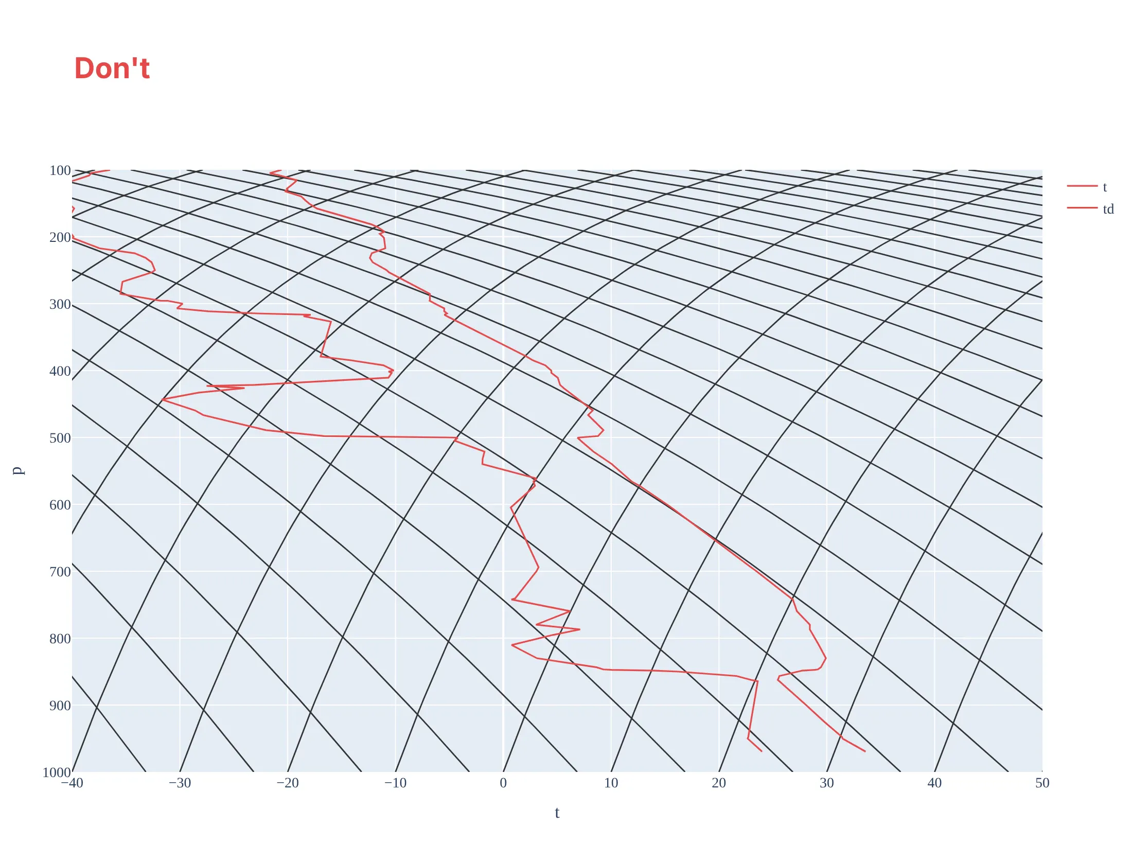
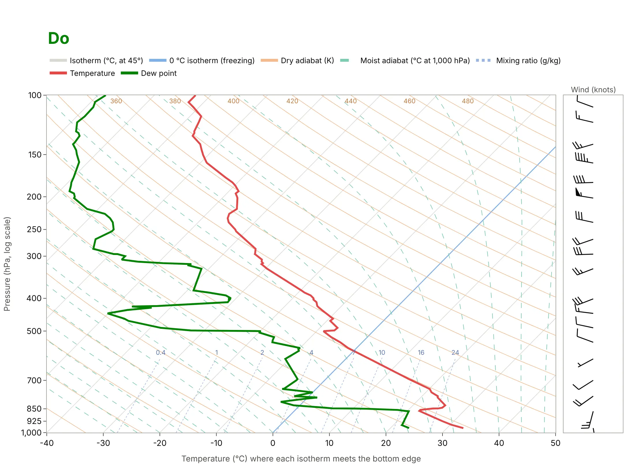
Most skew-T diagrams that are hard to read lose the one property that makes the chart work, which is that the isotherms and adiabats are straight, evenly spaced and cross at a large angle. Here is the same sounding both ways, with the same temperature color.
Don't put pressure on a linear axis (which curves every isotherm and breaks the diagram), draw temperature and dew point in the same color so they cannot be told apart, draw every background line in the same dark weight so the data disappears into the grid, leave the lines unlabeled, name the axes with column names ("t", "p") and no units, use a serif font on a tinted background, and leave out the wind:
Do use a log pressure axis with the standard levels as ticks, keep the background lines light so the red temperature and green dew point stand out, give the freezing line a different color, name the line families in a legend, put units on the axes, say that the x tick labels are read at the bottom edge, and draw the wind barbs in knots next to the chart:
Checklist
Do
- Use a log pressure axis, with 1,000 hPa at the bottom and tick labels at the standard levels.
- Set the skew so the isotherms are at 45 degrees on the screen, and tell readers to read temperatures at the bottom edge along the isotherm.
- Compute the adiabats, mixing ratio lines and parcel path with a tested package such as MetPy, not by hand.
- Draw temperature and dew point in two clearly different colors, and keep the background lines light.
- Say which parcel you lifted (surface-based, mixed-layer or most unstable) next to every CAPE and CIN value.
Don't
- Plot the same sounding on a linear pressure axis and call it a skew-T.
- Read a temperature straight down from a point on the chart; follow the isotherm to the bottom edge.
- Quote a CAPE value without the parcel and the time of the sounding, because it can range from 0 to thousands of J/kg on the same sounding.
- Draw the wind barbs without saying the unit (knots or meters per second).
More skew-T log-P diagram examples
Six more skew-T diagrams, each with its source, the technique that makes it work and a prompt to rebuild it. They show how the chart changes during a day, how the answer depends on the parcel, and what it says about island clouds, the top of the troposphere, aircraft icing and a whole season of soundings.
1. The cap weakens between morning and evening
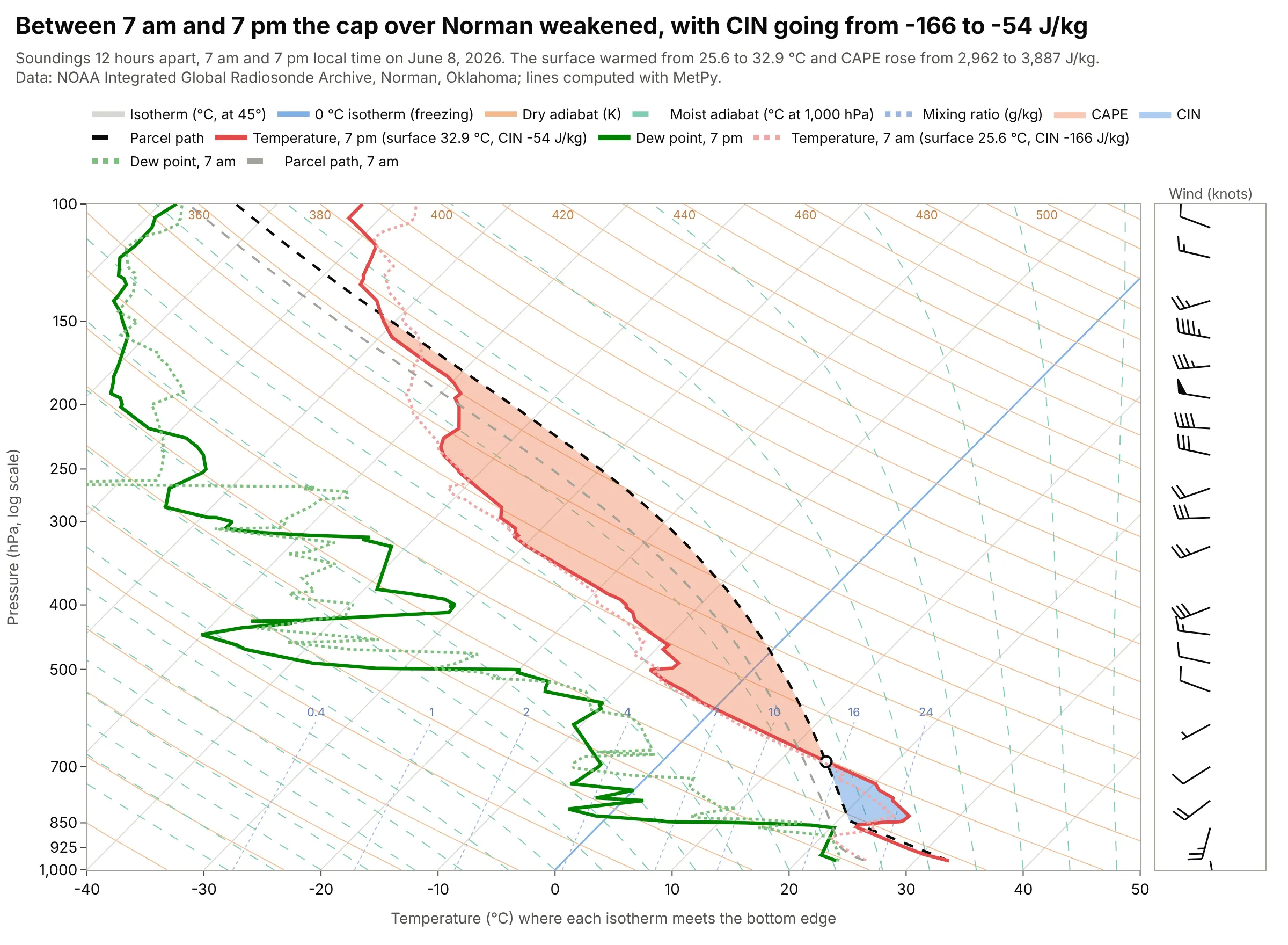
Between the 7 am and 7 pm soundings on June 8, 2026, Norman's surface warmed from 25.6 to 32.9 °C, the CIN went from -166 to -54 J/kg and the CAPE rose from 2,962 to 3,887 J/kg. A CIN closer to zero means less of a push is needed for the surface parcel to reach its LFC. Data: NOAA IGRA, Norman (station USM00072357), 12 UTC June 8 and 00 UTC June 9, 2026.
Tip: draw the earlier sounding pale and dotted and the later one bold, and put each one's surface temperature and CIN in the legend.
Get the data from NOAA's Integrated Global Radiosonde Archive (IGRA) version 2: the 2026 file for station USM00072357(Norman, Oklahoma), a fixed-width text file with one header line per sounding and one line per level (pressure in Pa,geopotential height in m, temperature in tenths of C, dew point depression in tenths of C, wind direction in degrees,wind speed in tenths of m/s). Keep the 12 UTC sounding of June 8 and the 00 UTC sounding of June 9, and convertto columns p_hpa, t_c, td_c, wdir_deg, wspd_kt.Make a plotly skew-T log-P diagram with metpy: the 00 UTC sounding bold with CAPE and CIN shaded, the 12 UTC soundingpale and dotted with its parcel path, and each sounding's surface temperature and CIN in the legend.
2. One sounding, three parcels, three answers
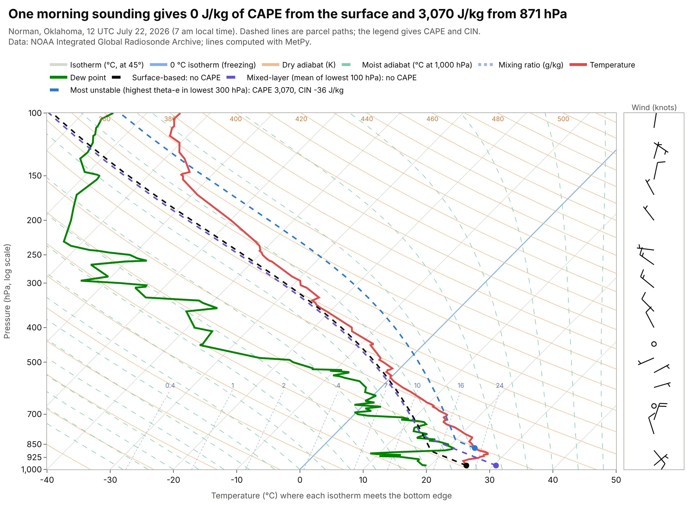
At 7 am local time on July 22, 2026, the surface-based and mixed-layer parcels at Norman had no CAPE at all, because the lowest layer was cooler than the air above it, while the most unstable parcel, lifted from 871 hPa, had 3,070 J/kg of CAPE and -36 J/kg of CIN. The mixed-layer parcel uses the average of the lowest 100 hPa and the most unstable parcel the level with the highest equivalent potential temperature in the lowest 300 hPa. Data: NOAA IGRA, Norman, 12 UTC July 22, 2026; parcels from MetPy's mixed_parcel and most_unstable_parcel.
Tip: name each parcel in the legend together with its CAPE and CIN, so no reader has to guess which one a number belongs to.
Get the data from NOAA's Integrated Global Radiosonde Archive (IGRA) version 2: the 2026 file for station USM00072357(Norman, Oklahoma), a fixed-width text file with one header line per sounding and one line per level (pressure in Pa,geopotential height in m, temperature in tenths of C, dew point depression in tenths of C, wind direction in degrees,wind speed in tenths of m/s). Keep the 12 UTC sounding of July 22 and convert to columns p_hpa, t_c, td_c.Make a plotly skew-T log-P diagram with metpy of the sounding with three dashed parcel paths: surface-based, mixed-layer(mixed_parcel, lowest 100 hPa) and most unstable (most_unstable_parcel, lowest 300 hPa), each in its own color withits CAPE and CIN in the legend and a dot where it starts.
3. Hilo's clouds stop under the summit of Mauna Kea
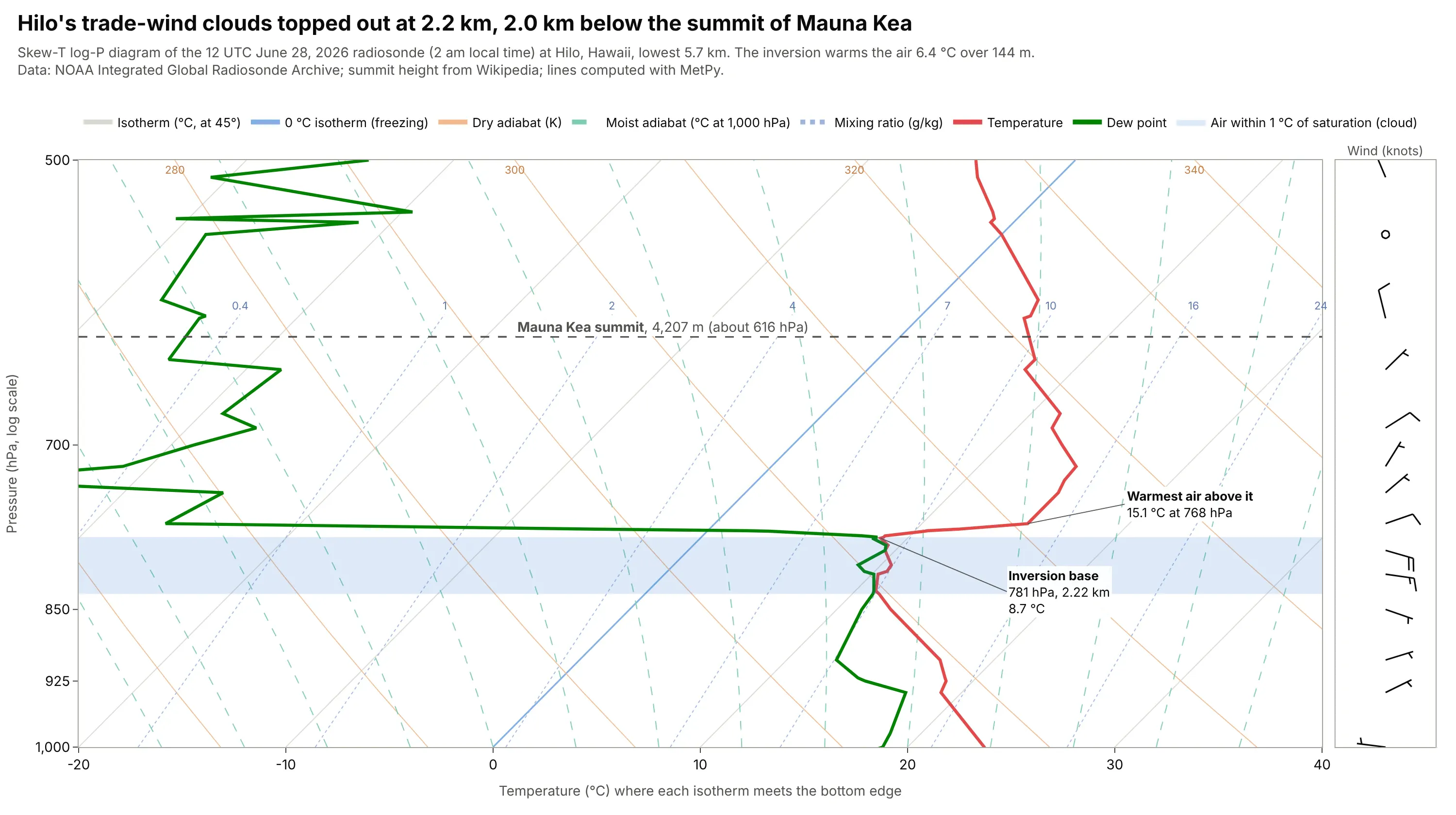
At Hilo the saturated layer ended at the inversion at 781 hPa, 2.22 km above sea level, where the temperature jumped from 8.7 to 15.1 °C in 144 m and the dew point fell from 8.3 to -26.5 °C. The summit of Mauna Kea, at 4,207 m or about 616 hPa, was 2.0 km above the cloud top (Wikipedia says the summit is above the inversion layer, and the Canada-France-Hawaii Telescope manual gives an average inversion height of 2,000 m). Data: NOAA IGRA, Hilo (station USM00091285), 12 UTC June 28, 2026; summit height from Wikipedia.
Tip: interpolate a landmark's height to a pressure with the sounding's own heights and draw it as a dashed line, so readers can see what is above or below it.
Get the data from NOAA's Integrated Global Radiosonde Archive (IGRA) version 2: the 2026 file for station USM00091285(Hilo, Hawaii), a fixed-width text file with one header line per sounding and one line per level (pressure in Pa,geopotential height in m, temperature in tenths of C, dew point depression in tenths of C, wind direction in degrees,wind speed in tenths of m/s). Keep the 12 UTC sounding of June 28 and convert to columns p_hpa, gph_m, t_c, td_c.Make a plotly skew-T log-P diagram with metpy from 1000 to 500 hPa, shade the layer where the dew point is within 1 Cof the temperature, interpolate the 4,207 m height of the Mauna Kea summit to a pressure from the sounding and draw it as adashed line, and label the inversion's base and the warmest air above it.
4. The tropopause is 6 km higher over Hilo than over Fairbanks
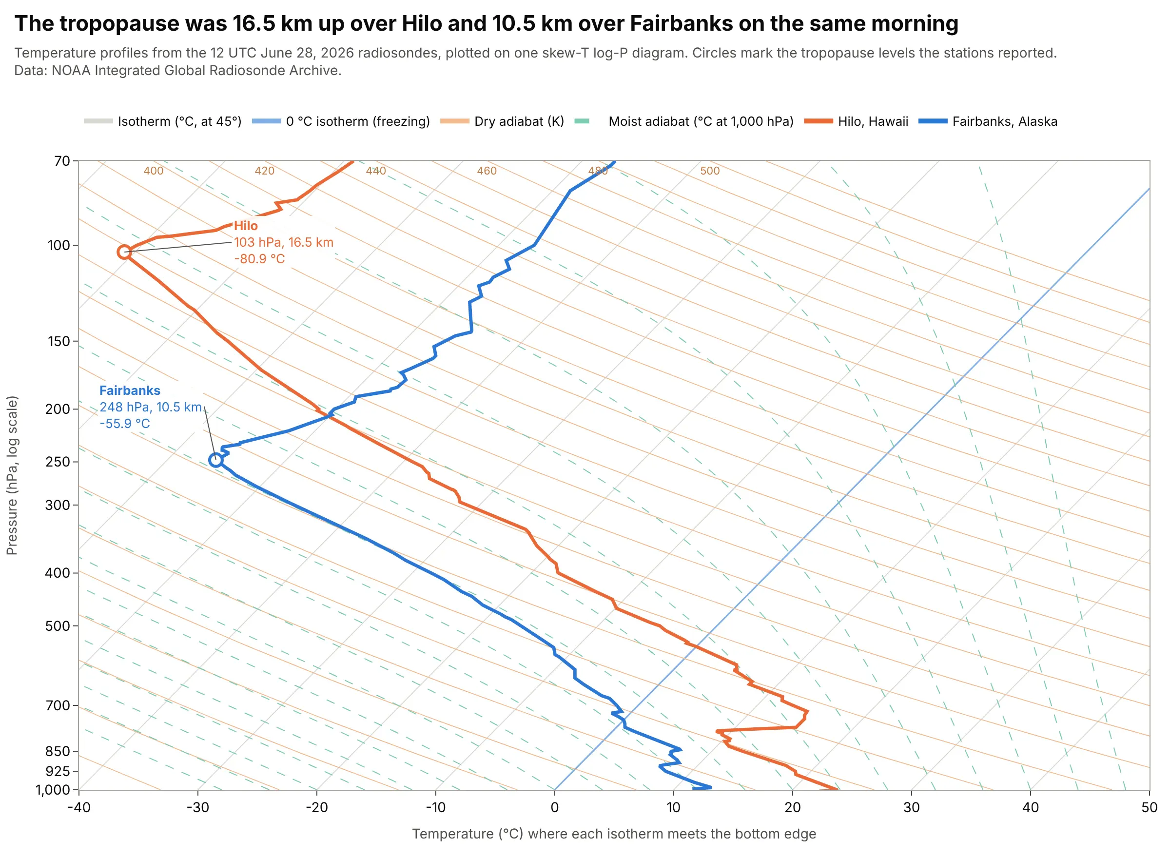
The tropopause, the top of the troposphere where the temperature stops falling with height, was reported at 103 hPa (16.5 km, -80.9 °C) over Hilo and at 248 hPa (10.5 km, -55.9 °C) over Fairbanks on the same June morning, so it was 6.0 km higher in the tropics. On a skew-T the line turns from leaning left to going vertical there. Data: NOAA IGRA, Hilo (USM00091285) and Fairbanks (USM00070261), 12 UTC June 28, 2026; tropopause levels as flagged in the archive.
Tip: plot only the temperature with one color per station when comparing places, and circle the tropopause each station reported.
Get the data from NOAA's Integrated Global Radiosonde Archive (IGRA) version 2: the 2026 files for station USM00091285(Hilo, Hawaii) and USM00070261 (Fairbanks, Alaska), fixed-width text files with one header line per sounding and one line perlevel (level type 2 in the second character marks the tropopause; pressure in Pa, geopotential height in m, temperaturein tenths of C). Keep the 12 UTC sounding of June 28 at both stations.Make a plotly skew-T log-P diagram with metpy-computed background lines from 1000 to 70 hPa, the two temperature profiles intwo colors, a circle at each station's tropopause level and a label with its pressure, height and temperature.
5. A cloud layer below freezing, and the jet stream above it
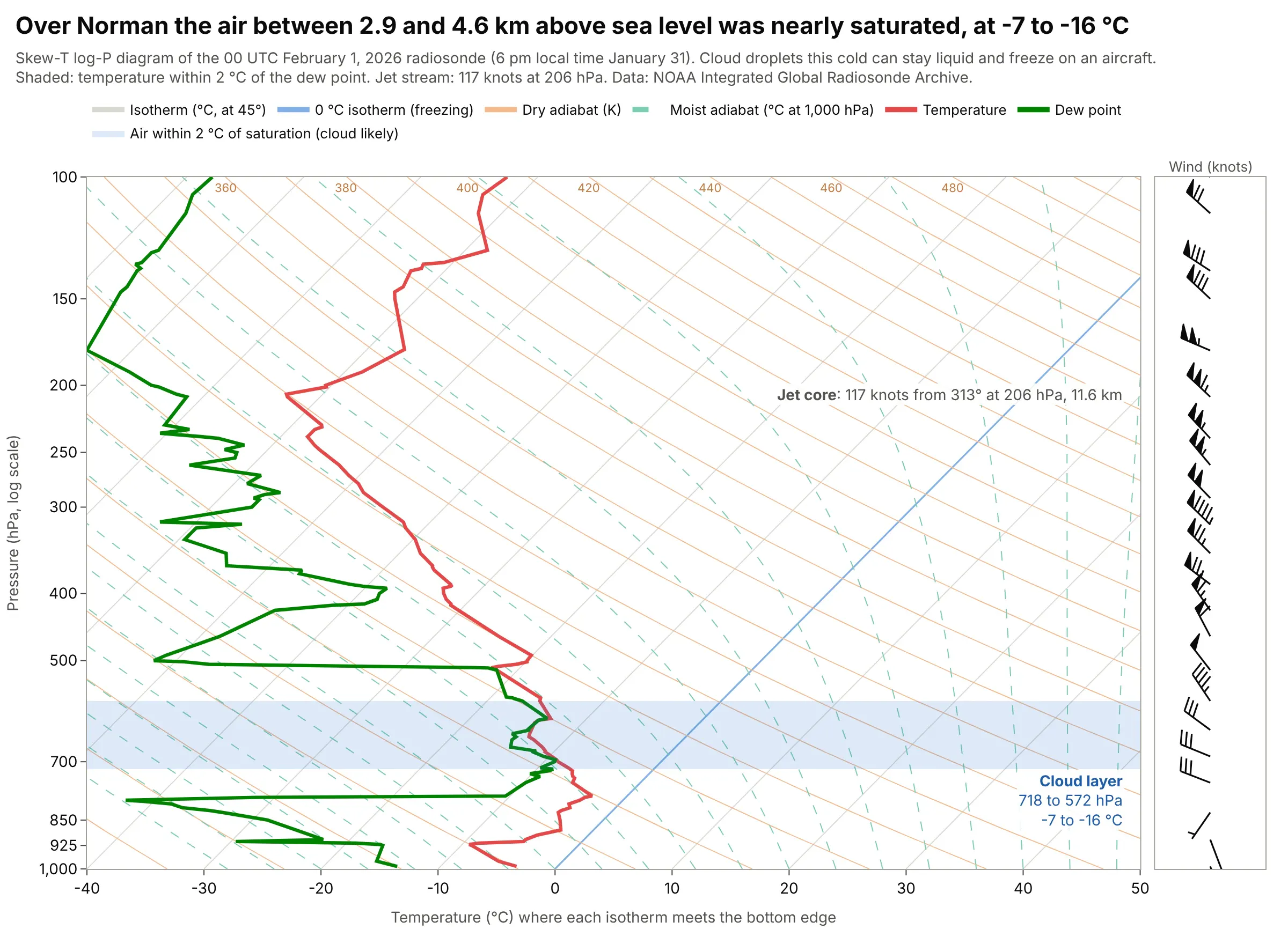
Over Norman on the evening of January 31, 2026, the temperature was within 2 °C of the dew point from 718 to 572 hPa (2.9 to 4.6 km above sea level), at -7.1 to -15.5 °C, and the wind peaked at 117 knots from 313 degrees at 206 hPa (11.6 km). Cloud droplets this cold can stay liquid and freeze on an aircraft, so pilots check the freezing line and the saturated layers on a skew-T first. Data: NOAA IGRA, Norman, 00 UTC February 1, 2026.
Tip: shade the saturated layer as a horizontal band across the whole chart and write its pressures and temperatures inside it.
Get the data from NOAA's Integrated Global Radiosonde Archive (IGRA) version 2: the 2026 file for station USM00072357(Norman, Oklahoma), a fixed-width text file with one header line per sounding and one line per level (pressure in Pa,geopotential height in m, temperature in tenths of C, dew point depression in tenths of C, wind direction in degrees,wind speed in tenths of m/s). Keep the 00 UTC sounding of February 1, 2026 and convert to p_hpa, gph_m, t_c, td_c,wdir_deg, wspd_kt.Make a plotly skew-T log-P diagram with metpy-computed background lines, shade the longest layer where the dew pointdepression is 2 C or less as a band, label its pressures and temperatures, label the strongest wind between 350 and150 hPa as the jet core, and draw wind barbs in knots on the right.
6. A whole summer of soundings on one chart
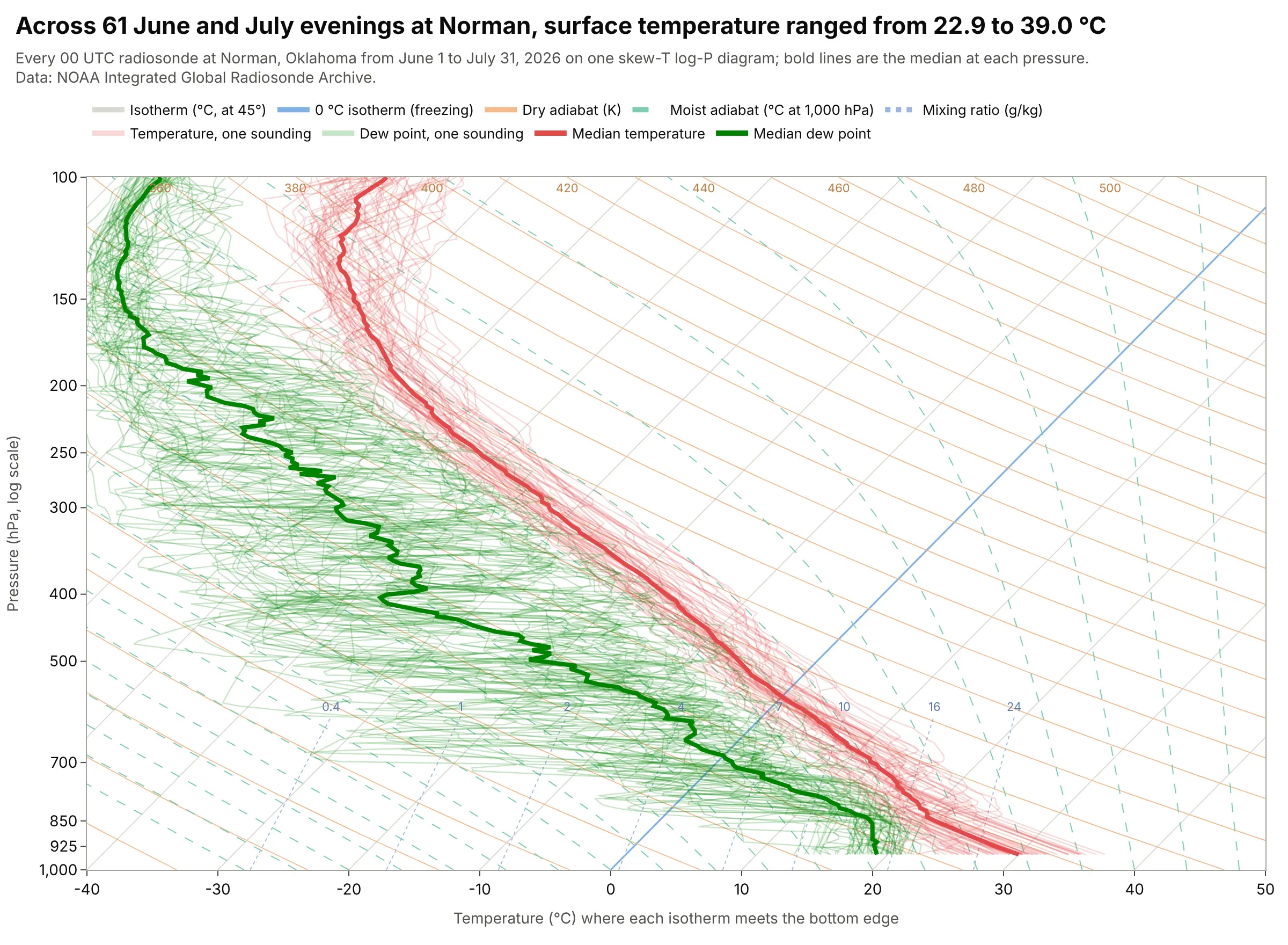
Across the 61 soundings from June 1 to July 31, 2026, Norman's surface temperature ranged from 22.9 to 39.0 °C, the 500 hPa temperature from -9.6 to -0.1 °C (median -5.7 °C) and the 850 hPa dew point from 6.4 to 19.4 °C (median 16.0 °C). The median soundings summarize the season, and the spread shows which levels vary most. Data: NOAA IGRA, Norman, every 00 UTC sounding from June 1 to July 31, 2026.
Tip: draw each sounding translucent and thin and the median bold, interpolating all soundings to the same pressure grid first.
Get the data from NOAA's Integrated Global Radiosonde Archive (IGRA) version 2: the 2026 file for station USM00072357(Norman, Oklahoma), a fixed-width text file with one header line per sounding and one line per level (pressure in Pa,temperature in tenths of C, dew point depression in tenths of C). Keep every 00 UTC sounding from June 1 to July 31.Make a plotly skew-T log-P diagram with metpy-computed background lines, every sounding's temperature and dew point as thintranslucent lines (interpolate to a common pressure grid in ln p), and the median temperature and median dew point at eachpressure as bold lines.
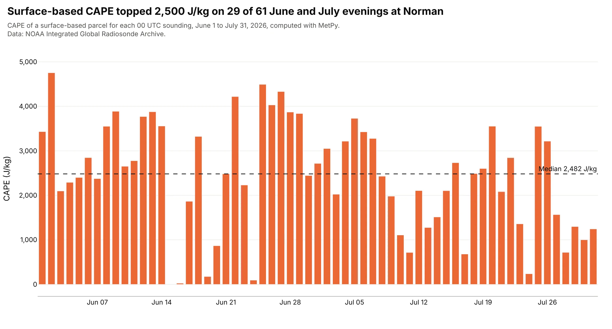
Another way to see it: the CAPE of the surface parcel for each of the 61 evenings, as a bar chart, shows that it exceeded 2,500 J/kg on 29 of them, with a median of 2,482 J/kg and a maximum of 4,753 J/kg on June 2, at the cost of every temperature and dew point detail.
FAQ
Options to customize
A skew-T in Plotly is a set of go.Scatter lines on a log pressure axis, so these are the options that matter most. The full lists are in the scatter trace reference, the axes documentation, the log axes documentation and the text and annotations documentation.
- fig.update_yaxes(type="log", range=[3, 2], tickvals=[...]): the log pressure axis with 1,000 hPa (log10 = 3) at the bottom and 100 hPa (log10 = 2) at the top, and tick labels at the standard levels.
- x = T + S * np.log(1000 / p): the skew itself, applied to every line; choose S from the plot's pixel size so the isotherms are at 45 degrees.
- go.Scatter(mode="lines", hoverinfo="skip"): one trace per background line, so hovering only shows the sounding.
- line=dict(color=..., width=..., dash=...): light isotherms, orange dry adiabats, dashed moist adiabats, dotted mixing ratio lines and heavy temperature and dew point lines.
- go.Scatter(fill="toself"): closed polygons for CAPE, CIN or a cloud layer between two curves.
- customdata and hovertemplate: show the real temperature and pressure in the hover, since the x value is skewed.
- fig.add_annotation(x=, y=, ax=, ay=, axref="x", ayref="y", arrowhead=0): labels with leader lines for the LCL, LFC, EL and other levels, in data coordinates (a log axis takes log10 of the pressure).
- fig.update_layout(xaxis2=dict(domain=[...]), yaxis2=...) with xaxis="x2", yaxis="y2" on a trace: a second panel for wind barbs drawn as lines, since Plotly has no barb trace.
- line=dict(color="rgba(227,73,72,0.22)"): translucent lines when you overlay many soundings, with the median bold.
- fig.update_layout(legend=dict(orientation="h")): a horizontal legend above the chart that names the line families.