Chris Parmer

November 9, 2026

Vector Field Plots - A Complete Guide

TL;DR

A vector field plot draws a quantity that has both a size and a direction, such as wind, an ocean current or a magnetic field, at many places at once: an arrow at each point shows which way it goes, and the arrow's length or color shows how strong it is.
Vector field plots are also known as quiver plots, vector plots and arrow plots, and when they trace the flow instead of drawing arrows, as streamline plots. They are similar to contour plots, which show the size of a field but not its direction, and to wind rose charts, which summarize the wind at one place over time. Wind barbs are a different, meteorological symbol for the same data.
The four forms Plotly draws are quiver plots (arrows at points), streamlines (curves that follow the flow), cone plots (3D arrows) and streamtubes (3D tubes that follow the flow from starting points you choose).
You can make a vector field plot with Plotly in Python from plotly.figure_factory.create_quiver and create_streamline in 2D, and the go.Cone and go.Streamtube traces in 3D.

What is a vector field plot?

Vector field plots look like this:

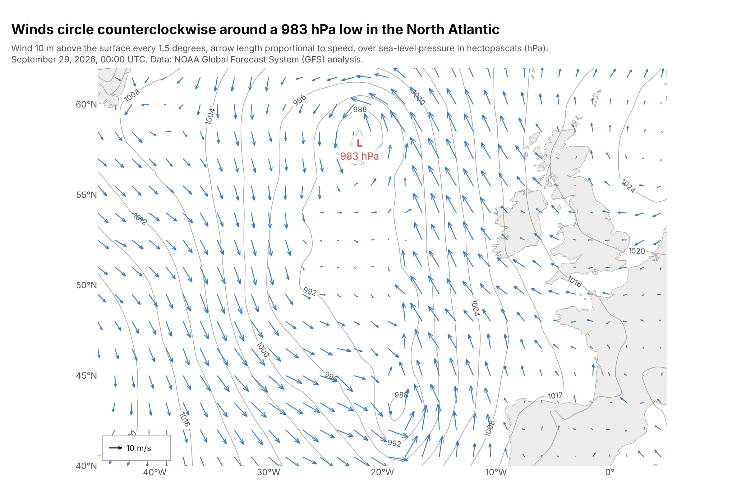
Quiver plot of 10 m winds over the North Atlantic on September 29, 2026: blue arrows every 1.5 degrees circle counterclockwise around a low of 983 hPa west of Ireland, over gray isobars, with the longest arrows south-east of the low and a 10 m/s key arrow in the corner

Data: US National Oceanic and Atmospheric Administration (NOAA), Global Forecast System (GFS) analysis, 0.25 degree grid.

How do you read a vector field plot? In the example above, notice these things:

Each of the 510 arrows is the wind 10 m above the surface at one grid point, every 1.5 degrees. It points the way the wind blows, and its length is proportional to the wind speed, so the 10 m/s arrow in the corner is the ruler for all the others.
The winds turn counterclockwise around the low of 983 hectopascals (hPa): at 57.5°N, the wind at 30°W, on the west side of the low, blows mostly south (v = −10.1 m/s), and at 15°W, on the east side, mostly north (v = 16.2 m/s).
The gray lines are isobars, lines of equal air pressure, every 4 hPa. Over the open ocean the arrows don't run exactly along them but cross them at about 15° toward the low, because friction with the sea surface slows the wind.
The longest arrows are south-east of the low, where the isobars bunch up. The fastest wind on the full grid is 21.8 m/s, at 48.75°N 17.5°W.

It's often used for charts like these:

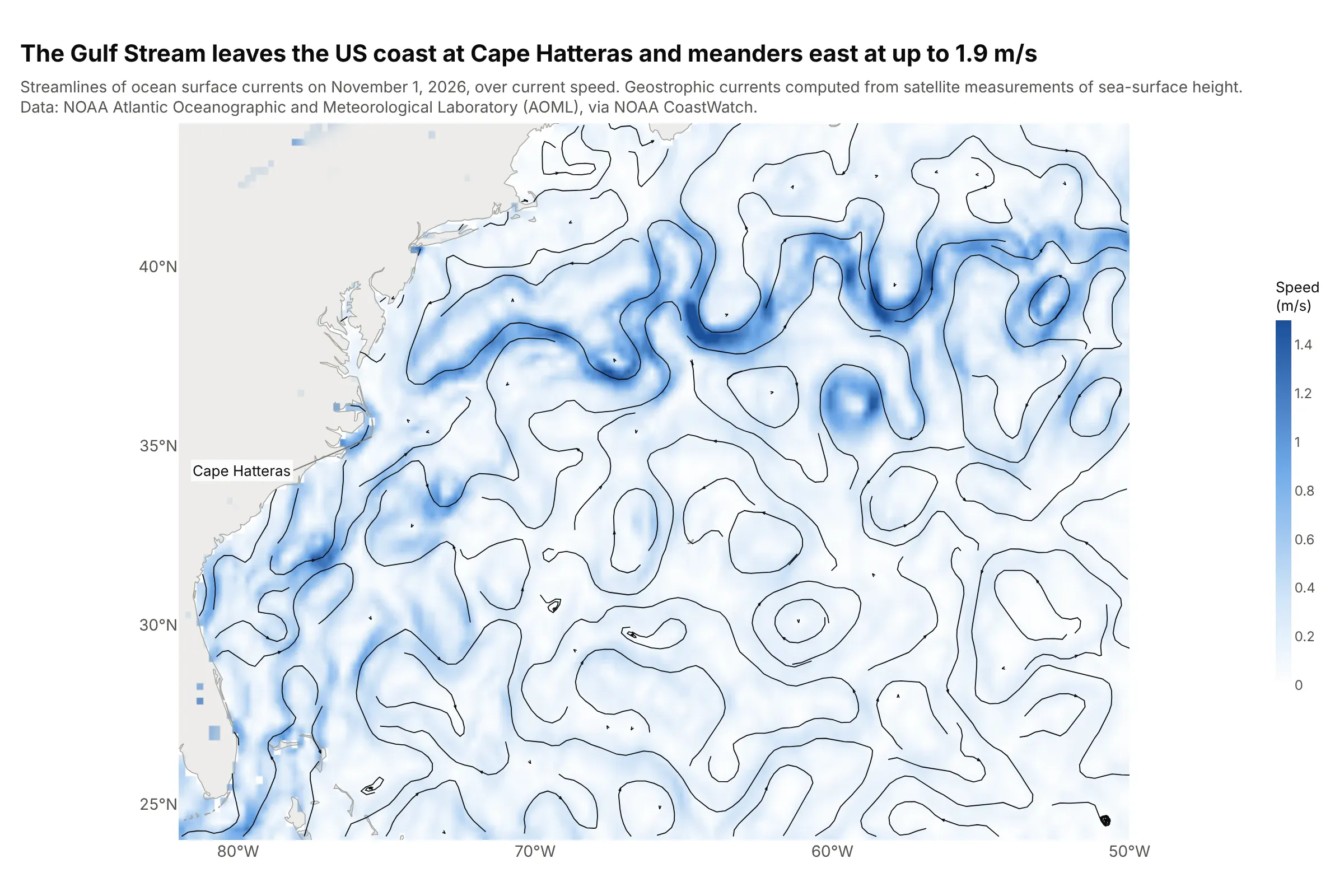
Streamlines of ocean surface currents off the US east coast on November 1, 2026, over a blue map of current speed: the Gulf Stream hugs the coast to Cape Hatteras, then meanders east in a dark blue band with eddies on both sides

Ocean currents. Streamlines follow the Gulf Stream from Florida past Cape Hatteras into the open Atlantic, where it meanders at up to 1.9 m/s and sheds eddies on both sides. Data: NOAA Atlantic Oceanographic and Meteorological Laboratory (AOML), near-real-time geostrophic currents from satellite altimetry, via NOAA CoastWatch.

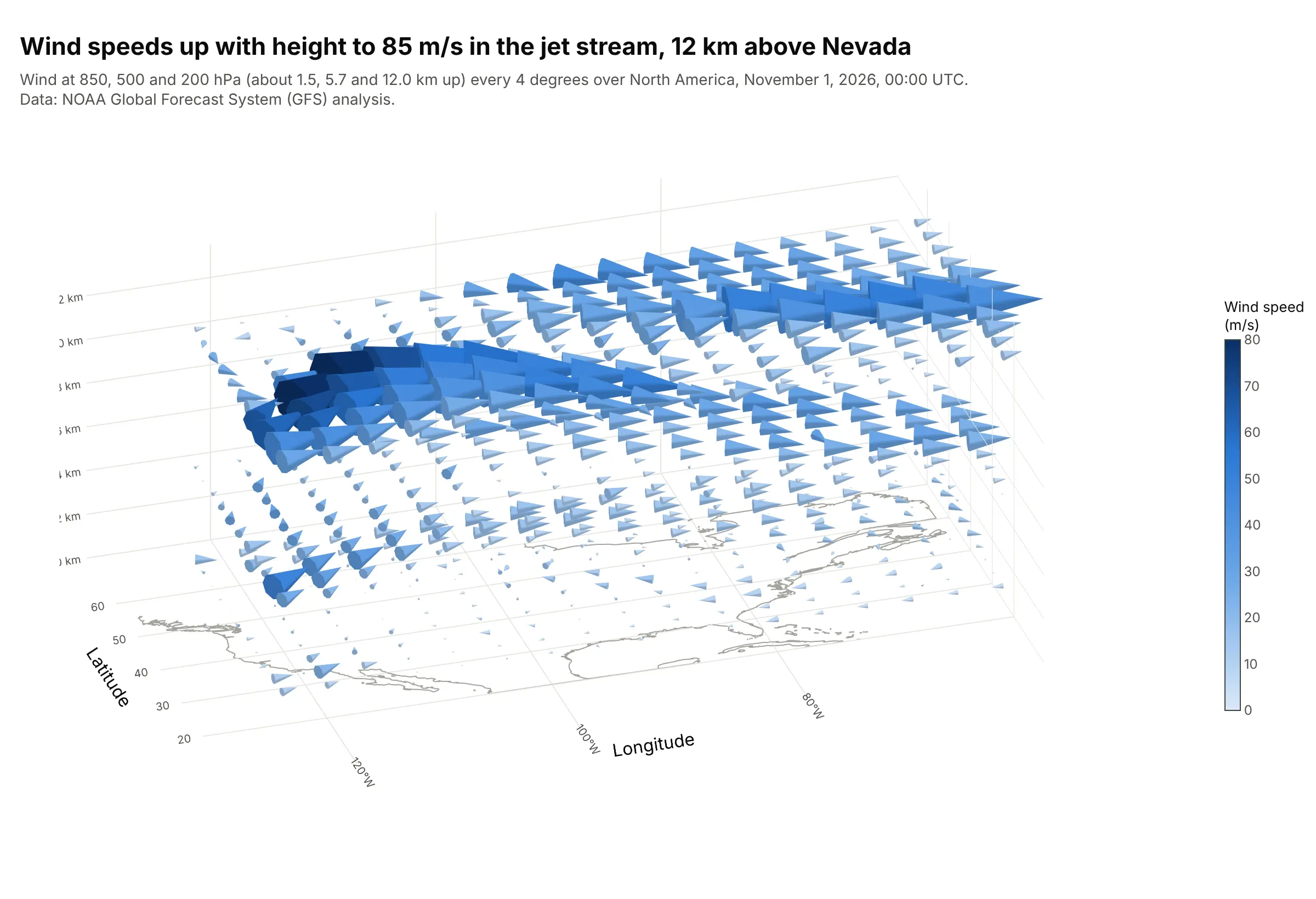
3D cone plot of winds over North America at 1.5, 5.7 and 12.0 km on November 1, 2026: small light cones near the ground and large dark blue cones at the top layer, where a band of fast eastward wind runs from Nevada across the continent

Winds in 3D. A cone plot shows the wind at three heights, and the fastest cones, up to 85 m/s, are in the jet stream 12 km above Nevada, where the average wind is five times the average near the ground. Data: NOAA GFS analysis at 11 pressure levels.

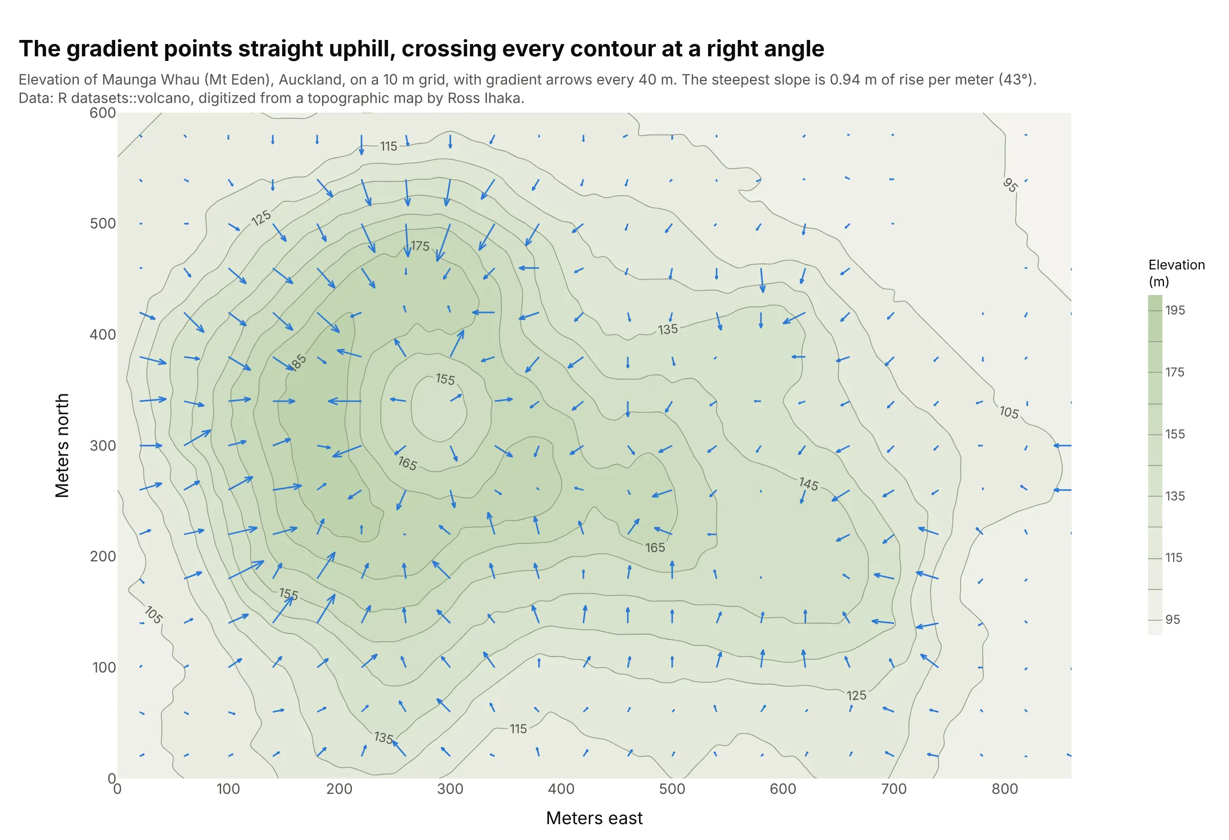
Quiver plot of the gradient of Maunga Whau volcano in Auckland over green filled contours of elevation: blue arrows point uphill, crossing the contour lines at right angles, longest on the steep outer slopes and pointing outward from the crater in the middle

The gradient of a surface, the classic textbook example. The arrows of a gradient point straight uphill and cross every contour at a right angle, longest where the slope is steepest, 0.94 m of rise per meter on this volcano. Data: R's volcano data set, Maunga Whau (Mt Eden), digitized from a topographic map by Ross Ihaka.

How to read a vector field: arrows, scale and streamlines

A vector field plot assumes a few ideas that are second nature to meteorologists and engineers but not to everyone. This section goes through them with the wind data from the first chart.

A vector has a direction and a size

Temperature or elevation is one number at each place, a scalar, and a heatmap or a contour plot can show it. Wind needs two numbers at each place, because it has a direction as well as a speed. Data files store it as two components: u, the speed toward the east (negative means toward the west), and v, the speed toward the north. This is the wind at 55°N 15°W from the first chart:

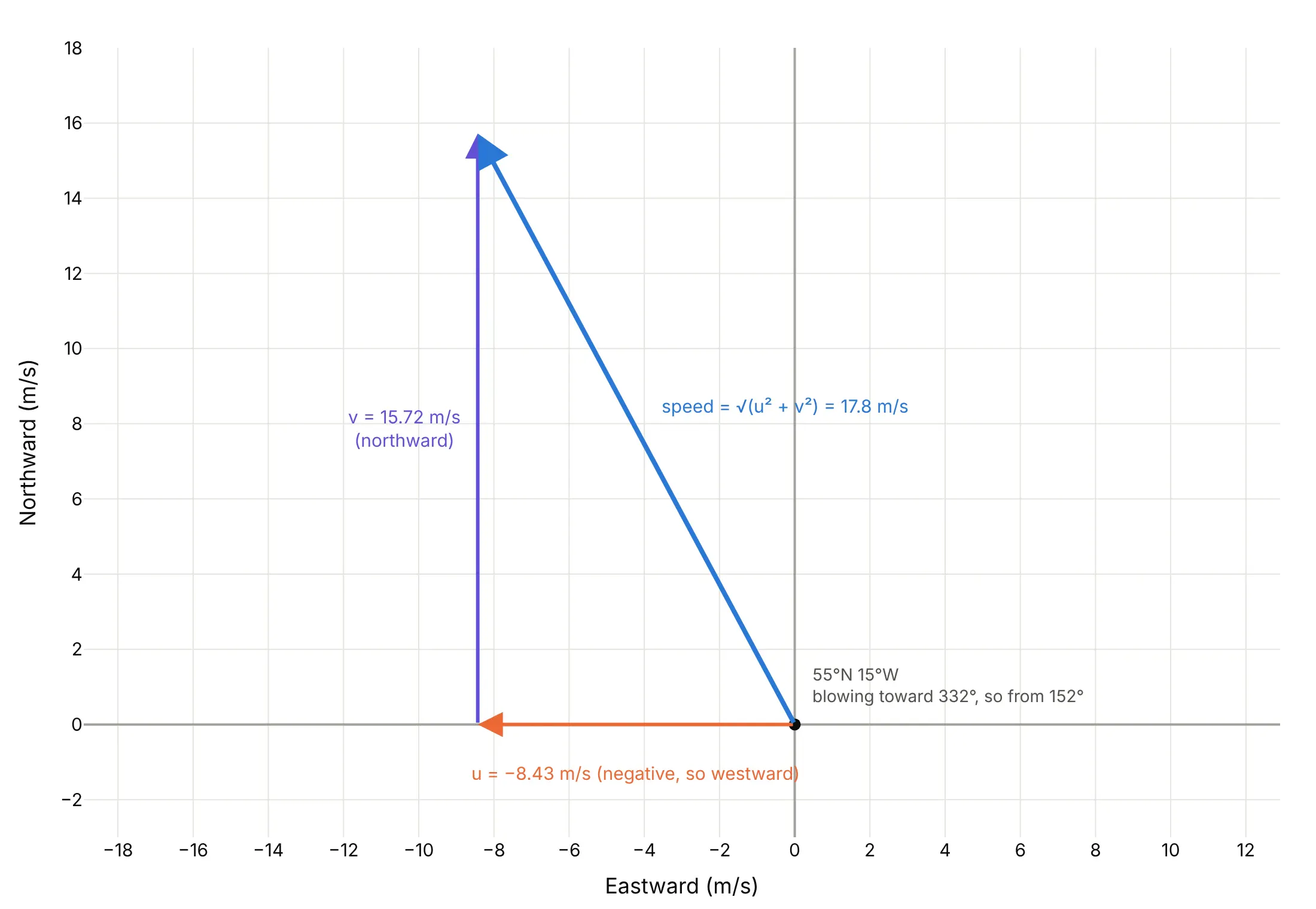
One wind vector drawn from the origin: an orange arrow of u = -8.43 m/s pointing left, a purple arrow of v = 15.72 m/s pointing up from its end, and a blue arrow from the origin to the same end point labeled speed = 17.8 m/s, blowing toward 332 degrees, so from 152 degrees

Data: NOAA GFS analysis, September 29, 2026, 00:00 UTC (Coordinated Universal Time).

The arrow is the two components added together: 8.43 m/s toward the west and 15.72 m/s toward the north make a wind of √(8.43² + 15.72²) = 17.8 m/s toward the north-northwest. A quiver plot draws that arrow at the place it was measured, scaled down to fit the map, and repeats it for every grid point. Meteorologists name a wind by where it comes from, so this one is a wind from 152°, a south-south-easterly. Keep that difference in mind when you turn a speed and a direction into u and v (the FAQ has the formula), because getting it backwards flips every arrow.

Arrow scaling

Arrow lengths have to be scaled from the data's units (m/s) into the plot's units (degrees of latitude here), and the right factor depends on how far apart the arrows are. create_quiver multiplies u and v by scale, and these are the same winds with three values of it:

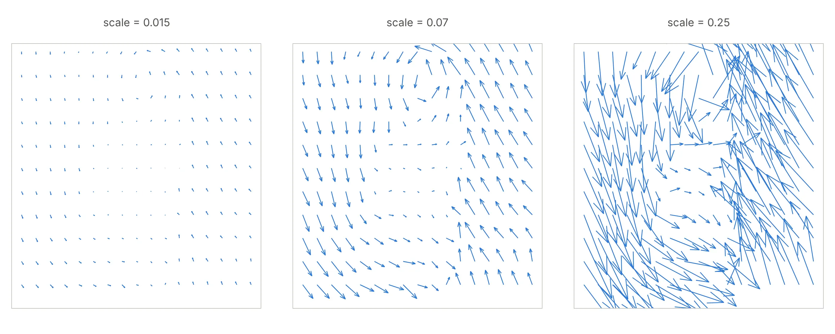
The same winds three times: with scale 0.015 the arrows are short ticks that hide the pattern, with scale 0.07 they are clear arrows that don't touch, and with scale 0.25 they are long lines that cross each other

Data: NOAA GFS analysis, the first chart's winds between 44°N and 60°N.

A good rule is to make the longest arrow a little shorter than the gap between two arrows, and to thin the grid (here every sixth point) rather than shrink the arrows until they're unreadable. On a map there is one more step. A degree of longitude is shorter than a degree of latitude, by a factor of cos(latitude), 0.63 at 51°N, so set the map's aspect with scaleratio = 1/cos(latitude) and pass the same scaleratio to create_quiver. Without it, the map is stretched east to west and every arrow points in a slightly wrong direction.

Streamlines and arrows

Arrows show the field at separate points. Streamlines are curves that are everywhere parallel to the field, so they show the paths it describes, like the swirls of iron filings around a magnet. A streamline plot is the better picture of flow (the Gulf Stream chart above), and a quiver plot is better when the value at each point matters or the data are scattered (example 2 below uses GPS stations). Streamlines don't show speed by their length, so add color, or read speed from how close together they are, which is what example 6 does.

Streamlines describe the field at one moment. In a flow that changes over time they are not the paths that real particles take (pathlines), and they coincide only when the flow is steady, as Wikipedia's article on streamlines, streaklines and pathlines explains.

3D: cones, sizemode and seeding streamtubes

In 3D, go.Cone is the arrow and go.Streamtube is the streamline. A cone's size is set by sizemode and sizeref. With "scaled" (the default), sizes are relative to the largest vector in the trace, so the biggest cone is about as long as the gap between points. With "absolute", sizeref is used as given, so two cone traces or animation frames with the same sizeref share one scale. With "raw", a cone is drawn exactly as long as its vector in the axis units.

A streamtube needs starting points, which you set with starts. Without them, plotly.js starts tubes on the face of the grid with the smallest y value, which for these winds is the southern edge at 20°N:

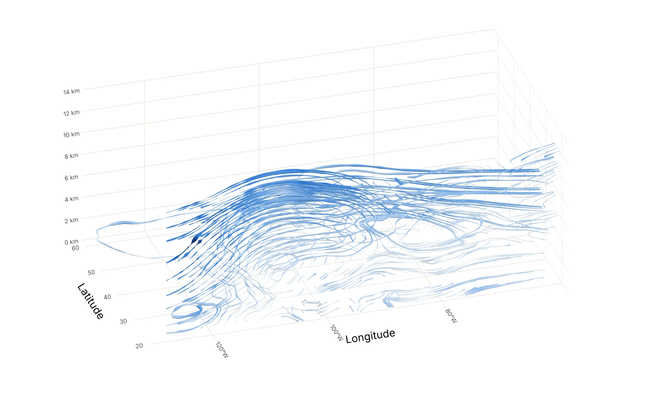
Streamtubes of the 3D wind field over North America with the default starting points: a dense tangle of thin light tubes starting along the southern face of the box, many turning and looping, with darker tubes bending north-east higher up

Data: NOAA GFS analysis, November 1, 2026, 00:00 UTC, 11 pressure levels.

The result is a tangle of tubes from the subtropics. Example 1 below passes 20 starting points on the west coast at four heights instead, which gives one readable tube per path. Choose starting points where the flow enters the region you care about, and use fewer than you think.

A short history

Edmond Halley drew what is generally considered the first meteorological map in 1686, a chart of the trade winds published with a paper on the trade winds and monsoons in the Philosophical Transactions of the Royal Society. Instead of arrows he drew rows of short strokes, "the sharp end of each little stroak pointing out that part of the Horizon, from whence the Wind continually comes", the same from-direction convention as today's wind barbs. Michael Faraday's lines of force, which iron filings make visible around a magnet, gave physics the streamline picture (Wikipedia). The name quiver plot comes from MATLAB's quiver function, a "Quiver or vector plot" in its documentation, and Matplotlib and Plotly use it too. plotly.js added 3D cone traces in version 1.38 (May 2018) and streamtubes in 1.39 (July 2018), according to its changelog. This is Halley's chart redrawn with eight years of satellite winds, in his style:

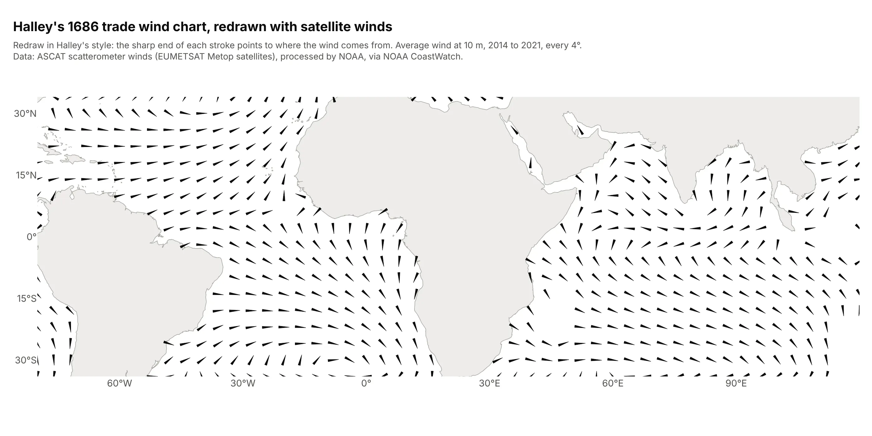
Halley-style map of the average surface wind over the tropical Atlantic and Indian Oceans from 2014 to 2021: rows of black tapered strokes with sharp ends toward the wind's source, showing north-easterly trades north of the equator and south-easterly trades south of it

Data: Advanced Scatterometer (ASCAT) winds from the European Metop satellites, processed by NOAA, via NOAA CoastWatch, monthly means averaged over 2014 to 2021.

The satellite averages show the same pattern Halley drew: between 10°N and 25°N in the Atlantic the average wind blows from 65° (the north-east trades) at 6.4 m/s, and between 10°S and 25°S from 113° (the south-east trades) at 6.1 m/s.

Alternatives to a vector field plot

Here's the same North Atlantic low drawn four ways. Some are better for the question, some worse, some just different:

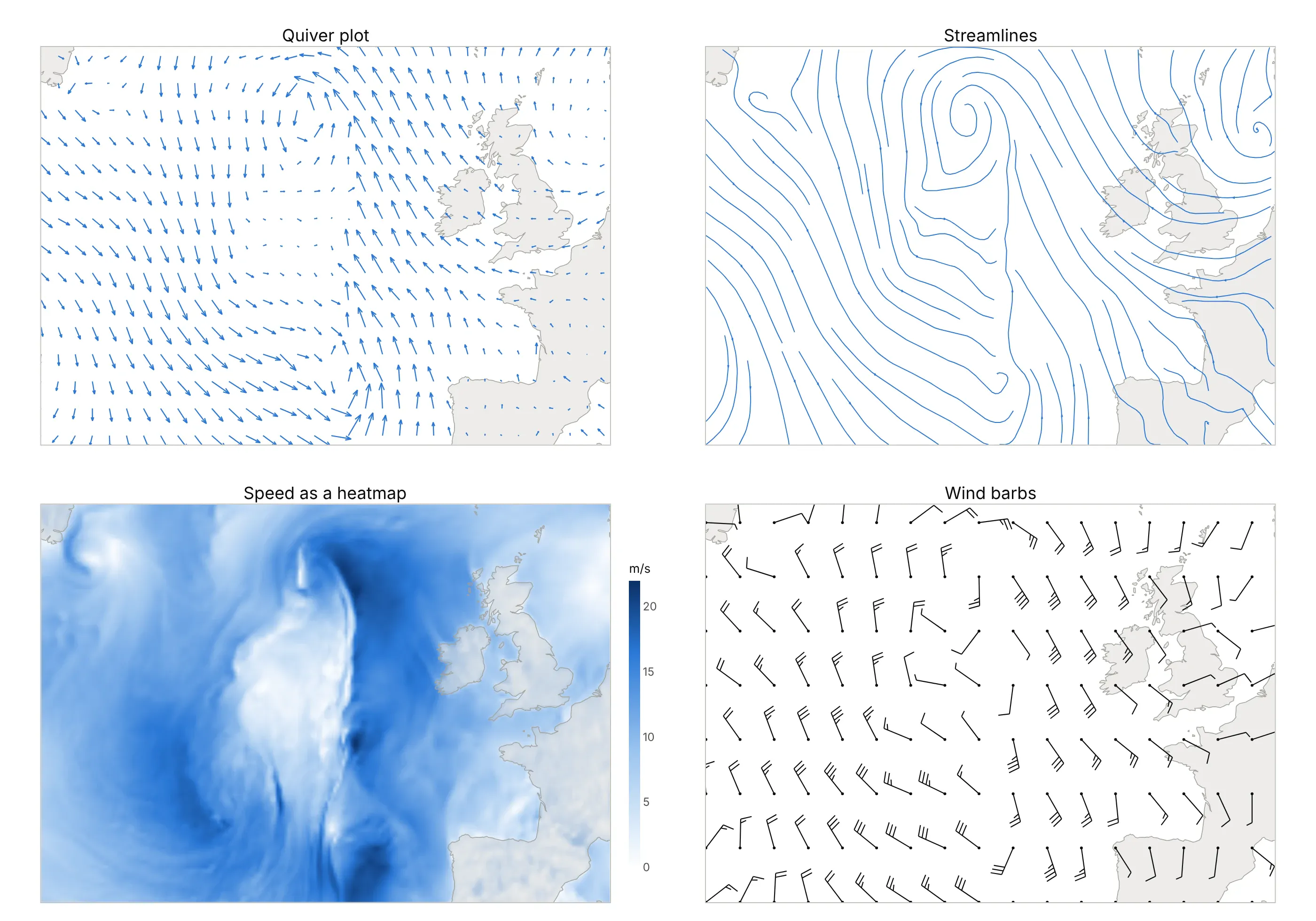
The North Atlantic winds of the first chart drawn four ways: a quiver plot with blue arrows, streamlines that spiral into the low, a blue heatmap of wind speed with no direction, and black wind barbs with feathers counting knots

Quiver plot (the default). Arrows show direction and speed at every point and work for scattered data, but they get crowded, and the eye has to join them up to see the circulation.
Streamlines (better for flow). The spiral into the low is obvious at once, but speed is gone unless you add color, and create_streamline needs a regular grid.
Heatmap or contour plot of speed (worse for direction, better for magnitude). It shows exactly where the wind is strongest, which matters most for wind energy (example 4), but not which way it blows. Combine it with arrows or streamlines.
Wind barbs (different). The meteorological convention: the staff points to where the wind comes from, and each long feather is 10 knots, a short one 5 and a flag 50, as the US National Weather Service explains. Barbs give speed to the nearest 5 knots, which forecasters read easily and most other audiences don't. You can draw them with Plotly as line segments, as this figure does.
Wind rose (different). It shows how often the wind blows from each direction at one place over months, instead of everywhere at one time.
3D cones or streamtubes (for 3D fields). Use them when height matters, as in the cone plot above and example 1 below; for a single layer a 2D plot is easier to read. A 3D surface plot shows a scalar over a plane in 3D, not a vector.

How to make a vector field plot

With AI

ChatGPT, Claude Code, GitHub Copilot, Cursor and other AI tools are excellent at writing Plotly code. Name Plotly in the prompt, and say how the components are stored and how to scale the arrows:

Make a plotly quiver plot from winds.csv (columns: lat, lon, u, v; u is the eastward and v the northward
wind in m/s, on a 0.25 degree grid).

- Use plotly.figure_factory.create_quiver with an arrow every 1.5 degrees, scale so the longest arrow is a
  little shorter than the 1.5 degree spacing, and scaleratio = 1/cos(mean latitude) so the map isn't stretched.
- Add a 10 m/s key arrow in a corner and light gray land outlines from Natural Earth.
- Put sea-level pressure (column mslp_hpa) underneath as gray contour lines every 4 hPa with labels.
- A title that states the takeaway.
- Check: print the maximum wind speed and where it is.

With Plotly Studio

Plotly Studio is a desktop app where you point an AI at a dataset and it builds charts and a Dash app around your questions. Ask for a vector field plot the same way:

Show the surface winds as a quiver plot over a heatmap of wind speed, with a slider for the time step and a dropdown to switch between arrows and streamlines.

Make a vector field plot in Python or JavaScript

This is the code AI tools write under the hood. In Python, create_quiver takes the arrow positions and components and returns a figure with one line trace for all the arrows:

import numpy as np
import pandas as pd
import plotly.figure_factory as ff

df = pd.read_csv("winds.csv")  # lat, lon, u, v (m/s), one row per grid point
df = df[(df.lat % 1.5 == 0) & (df.lon % 1.5 == 0)]  # an arrow every 1.5 degrees
r = 1 / np.cos(np.radians(df.lat.mean()))  # a degree of longitude is shorter than a degree of latitude

fig = ff.create_quiver(df.lon, df.lat, df.u, df.v, scale=0.07, arrow_scale=0.3, scaleratio=r, line_width=1.2)
fig.update_layout(xaxis_title="Longitude", yaxis_title="Latitude")  # scaleratio also sets the axes' aspect
fig.show()

create_quiver loops in pure Python, which is fine for the few hundred arrows a readable map needs but takes about a minute for 10,000 (see the FAQ). For more, build the same arrows with numpy and draw them as one go.Scattergl line trace:

import plotly.graph_objects as go

def quiver_lines(x, y, u, v, scale=0.1, arrow_scale=0.3, angle=np.pi / 9):
    """The shafts and heads create_quiver draws, as x and y arrays with NaN gaps, for any number of arrows."""
    x, y, u, v = (np.asarray(a, float).ravel() for a in (x, y, u, v))
    x1, y1 = x + u * scale, y + v * scale
    ang, head = np.arctan2(v, u), arrow_scale * np.hypot(u, v) * scale
    gap = np.full_like(x, np.nan)
    xs = np.column_stack([x, x1, gap, x1 - head * np.cos(ang + angle), x1, x1 - head * np.cos(ang - angle), gap])
    ys = np.column_stack([y, y1, gap, y1 - head * np.sin(ang + angle), y1, y1 - head * np.sin(ang - angle), gap])
    return xs.ravel(), ys.ravel()

xs, ys = quiver_lines(df.lon, df.lat, df.u, df.v, scale=0.07)
fig = go.Figure(go.Scattergl(x=xs, y=ys, mode="lines", line_width=1))

On a map, multiply u by the same r as above before calling it and set scaleanchor="x", scaleratio=r on the y axis.

create_streamline takes 1D x and y and 2D u and v. Its x and y must be evenly spaced and of the same length, and the speed can't be zero anywhere, so fill land or empty cells with a tiny value:

grid = pd.read_csv("currents.csv")  # lat, lon, u, v on an evenly spaced grid with as many lons as lats
x = np.sort(grid.lon.unique()); y = np.sort(grid.lat.unique())
U = grid.pivot(index="lat", columns="lon", values="u").fillna(1e-6).values
V = grid.pivot(index="lat", columns="lon", values="v").fillna(0).values
fig = ff.create_streamline(x, y, U, V, density=1.5, arrow_scale=0.1)

In 3D, go.Cone and go.Streamtube take flat columns of positions and components. The streamtube's points must form a full regular grid (the spacing can vary along an axis, as the heights do here):

import plotly.graph_objects as go

w3 = pd.read_csv("winds_3d.csv")  # lon, lat, z_km, u, v: every combination of the grid's lon, lat and z_km
fig = go.Figure(go.Cone(x=w3.lon, y=w3.lat, z=w3.z_km, u=w3.u, v=w3.v, w=0 * w3.u,
                        sizemode="absolute", sizeref=22, anchor="tail", colorscale="Blues"))
fig.add_trace(go.Streamtube(x=w3.lon, y=w3.lat, z=w3.z_km, u=w3.u, v=w3.v, w=0 * w3.u,
                            starts=dict(x=[-128] * 4, y=[36, 40, 44, 48], z=[9] * 4), sizeref=0.6))
fig.update_layout(scene=dict(aspectmode="manual", aspectratio=dict(x=2, y=1.2, z=0.8)))
fig.show()

In JavaScript, plotly.js draws a quiver plot as one line trace once you compute each arrow's shaft and head:

<div id="chart"></div>
<script src="https://cdn.plot.ly/plotly-4.1.1.min.js"></script>
<script>
  // NOAA GFS 10 m winds (m/s) over the North Atlantic, September 29, 2026, 00:00 UTC
  const lat = [45, 45, 45, 45, 45, 50, 50, 50, 50, 50, 55, 55, 55, 55, 55, 60, 60, 60, 60, 60];
  const lon = [-40, -30, -20, -10, 0, -40, -30, -20, -10, 0, -40, -30, -20, -10, 0, -40, -30, -20, -10, 0];
  const u = [3.85, 12.44, 7.97, -3.96, -1.15, 7.28, 4.22, 1.89, -9.2, -8.67, 8.37, 1.37, 3.82, -7.82, -3.94, -4.68, -1.52, -15.17, -4.25, 0.45];
  const v = [-10.43, -11.06, -6.97, 10.78, 2.46, -9.76, -12.69, 0.38, 7.63, 2.46, -6.45, -11.9, 4.17, 11.69, 3.09, 0.56, -7.17, 7.78, 10.99, 4.68];
  const scale = 0.25, r = 1 / Math.cos(52.5 * Math.PI / 180);  // degrees per m/s, and the map's aspect
  const x = [], y = [];
  lat.forEach((la, i) => {
    const dx = u[i] * scale, dy = v[i] * scale, x1 = lon[i] + dx * r, y1 = la + dy;
    const ang = Math.atan2(dy, dx), head = 0.3 * Math.hypot(dx, dy);
    x.push(lon[i], x1, null, x1 - head * Math.cos(ang - 0.35) * r, x1, x1 - head * Math.cos(ang + 0.35) * r, null);
    y.push(la, y1, null, y1 - head * Math.sin(ang - 0.35), y1, y1 - head * Math.sin(ang + 0.35), null);
  });
  Plotly.newPlot("chart", [{x: x, y: y, mode: "lines", line: {color: "#2a78d6", width: 2}}], {
    width: 800, height: 520,
    xaxis: {title: {text: "Longitude"}},
    yaxis: {title: {text: "Latitude"}, scaleanchor: "x", scaleratio: r}
  });
</script>

For a 3D field in JavaScript, use type: "cone" or type: "streamtube" with the same x, y, z, u, v and w arrays as in Python.

Share it

Every Plotly chart has a Share chart button (the cloud icon in its toolbar) that uploads it to Plotly Cloud and gives you a link. Only you can see it until you change its visibility.

For a live app, put the chart in a Dash app and publish it with the Plotly Cloud command-line interface (CLI). Coding agents can run these commands for you:

pip install "dash[cloud]"
plotly user login
plotly app publish

If your data has to stay in your own cloud or data center, publish to Dash Enterprise instead.

Dos and don'ts

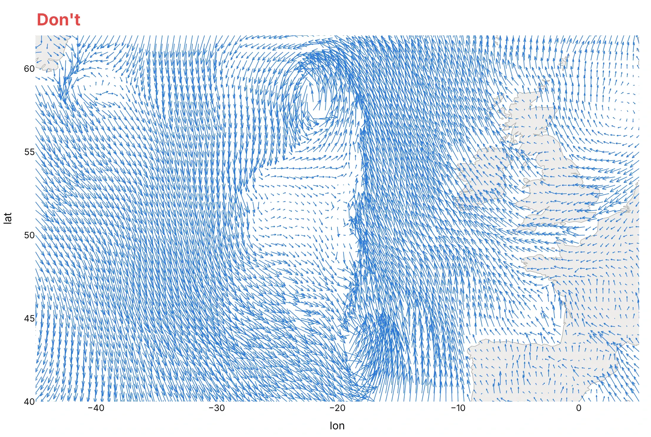
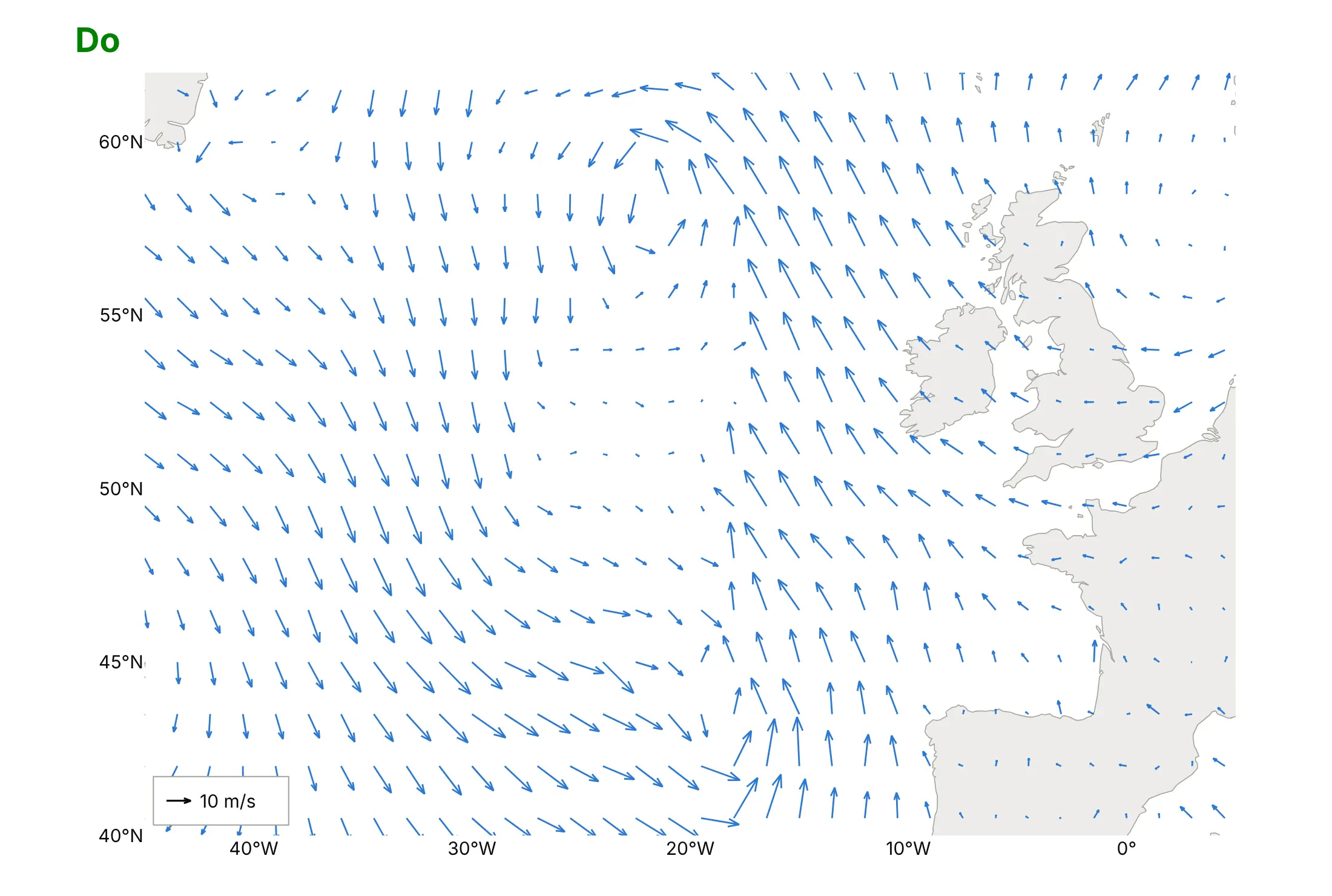
Most quiver plots go wrong in the same three places: too many arrows, the wrong aspect ratio and no scale. Here are the North Atlantic winds both ways, in the same color.

Don't draw an arrow at every grid point with a scale that makes them overlap, let the map stretch to fill the frame (without scaleanchor and scaleratio every arrow's angle is wrong), or leave out a key for the arrow length:

The North Atlantic winds with an arrow every 0.5 degrees, so dense that they merge into a blue texture, on a map stretched east to west, with axis titles lon and lat and no key

Do thin the arrows until they don't touch, keep the map in proportion with scaleratio = 1/cos(latitude) (and pass it to create_quiver), add a key arrow, and label the axes in degrees:

The same winds with an arrow every 1.5 degrees, the map in proportion, a 10 m/s key arrow in a white box in the corner, and axes labeled 40 degrees W to 0 and 40 to 60 degrees N

Checklist

Check the components: u is eastward and v northward, and wind directions in data files are usually where the wind comes from.
Thin a dense grid (every nth point) and scale the longest arrow to a bit less than the spacing.
Keep x and y in proportion with scaleanchor, and on a map use scaleratio = 1/cos(latitude).
Add a key arrow, or color by speed with a titled colorbar.
Put the scalar that explains the field underneath: isobars under wind, elevation under a gradient, speed under currents.
Seed streamtubes yourself with starts, where the flow enters.

Don't

Use length for speed when speeds span a factor of 100; use arrows of one length and color for speed (example 4).
Draw streamlines across land or empty areas; cut them where there is no data.
Compare cone sizes between traces with sizemode="scaled", which rescales each trace to its own largest vector.

Options to customize

A 2D vector field plot in Plotly is a line trace built by the figure factory, and a 3D one is a cone or streamtube trace, so these are the options that matter most. The full lists are in the quiver, streamline, cone trace and streamtube trace references.

ff.create_quiver(x, y, u, v, scale=...): arrows at any points, gridded or scattered; scale turns data units into axis units.
arrow_scale and angle: the arrowhead's length as a share of the arrow (default 0.3) and its half-angle in radians (default 0.35, 20°).
scaleratio in create_quiver: keeps arrow angles and heads right when the y axis is drawn at a different scale, and sets yaxis.scaleanchor for you.
ff.create_streamline(x, y, u, v, density=...): streamlines on an evenly spaced grid with x and y of equal length; density sets how many lines.
line_color, line_width and hoverinfo: the figure factories pass these to the line trace; add an invisible marker trace at the arrow tails for hover values.
go.Cone(sizemode=...): "scaled" (relative to the largest vector), "absolute" (sizeref used as given, for a scale shared across traces) or "raw" (cones as long as the vector, added in plotly.js 2.31).
sizeref and anchor: cone size and whether the cone's "tail", "tip", "center" or "cm" (center of mass) sits on the point.
go.Streamtube(starts=dict(x=..., y=..., z=...)): where the tubes begin; without it they start on the face of the grid with the smallest y.
maxdisplayed and sizeref on streamtubes: the maximum number of segments drawn per tube (default 1000; a small value cuts tubes short) and the tube width scale.
colorscale, cmin, cmax, colorbar: color by speed (the norm of u, v, w) on cones and streamtubes; set cmin and cmax to compare plots.
hovertemplate with %{norm}, %{u}, %{v}, %{w} (and %{divergence} on streamtubes): hover labels with the speed and components.
scene.aspectmode, aspectratio and camera.projection.type="orthographic": proportions of a 3D box when axes have different units, and a view without perspective that keeps near cones from hiding the axes.

More vector field plot examples

Six more vector field plots, five from real public data and one computed from a formula, each with its source, the technique that makes it work and a prompt to rebuild it.

1. The jet stream as streamtubes

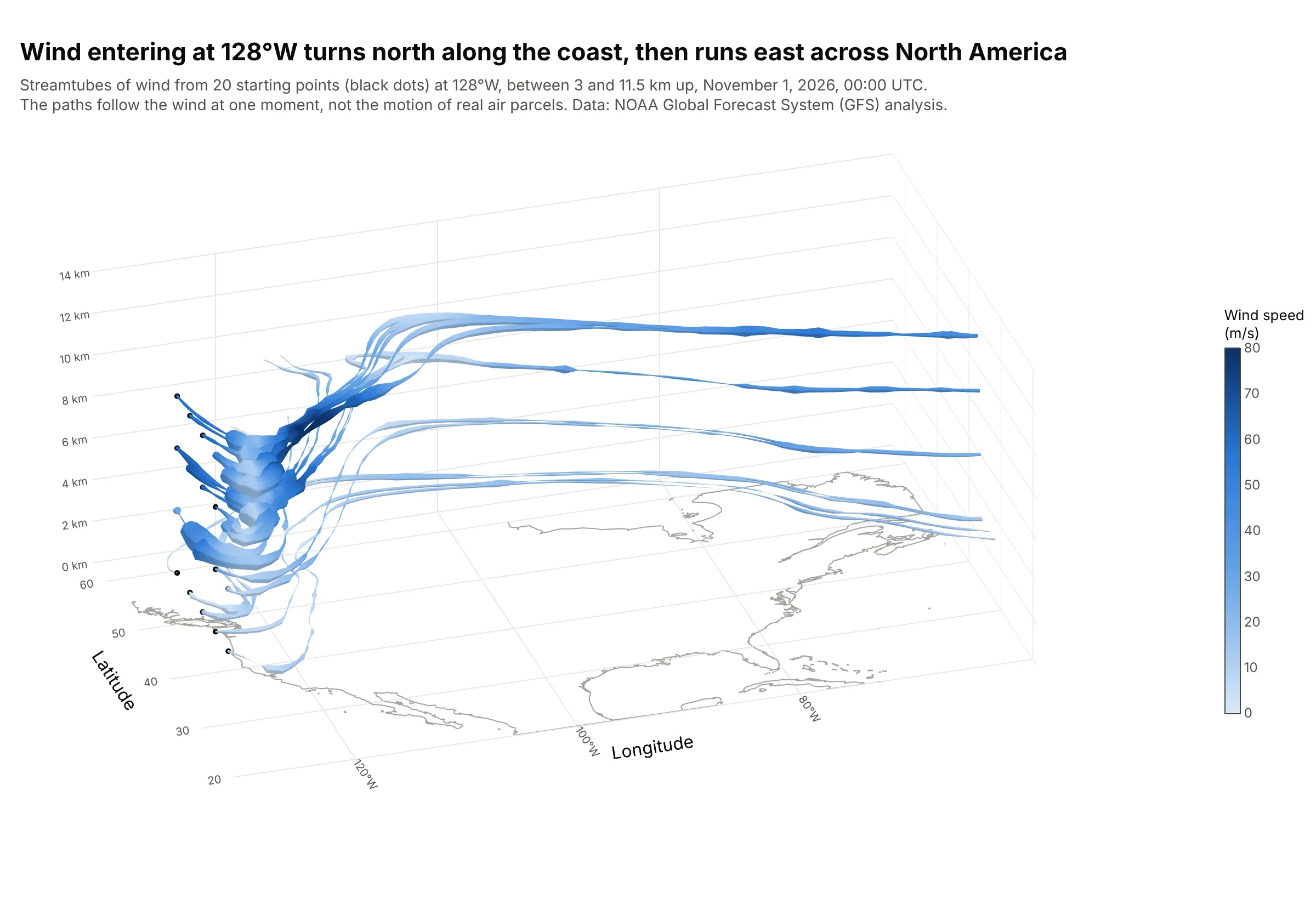
Streamtubes of the wind over North America from 20 black starting points at 128 degrees W between 3 and 11.5 km: they bend north along the coast, then run east across the continent, the fastest parts in dark blue

Twenty tubes start off the Pacific coast at 128°W at four heights, turn north along the coast and then run east across the continent in the jet stream, whose core reaches 85 m/s. plotly.js sets each tube's width from the divergence of the flow, how fast it spreads out or squeezes together. Data: NOAA GFS analysis, November 1, 2026, 11 pressure levels every 2 degrees.

Tip: pass starts with a few points where the flow enters, and draw them as markers so readers see where each tube begins.

Get the data from the NOAA Global Forecast System (GFS) 0.25 degree analysis for 2026-11-01 00 UTC on the NOAA
Open Data Dissemination archive on AWS (noaa-gfs-bdp-pds): UGRD, VGRD and HGT at 1000, 925, 850, 700, 600, 500,
400, 300, 250, 200 and 150 hPa, 20N to 60N and 130W to 60W, every 2 degrees, each level at its mean height in km
(columns: lon, lat, z_km, u, v).

Build a plotly go.Streamtube with w = 0, starts at 128W for latitudes 32 to 48 every 4 degrees and heights 3, 6, 9
and 11.5 km, colored by speed from 0 to 80 m/s, the starting points as black markers and an orthographic camera.

2. California drifting north-west, from GPS stations

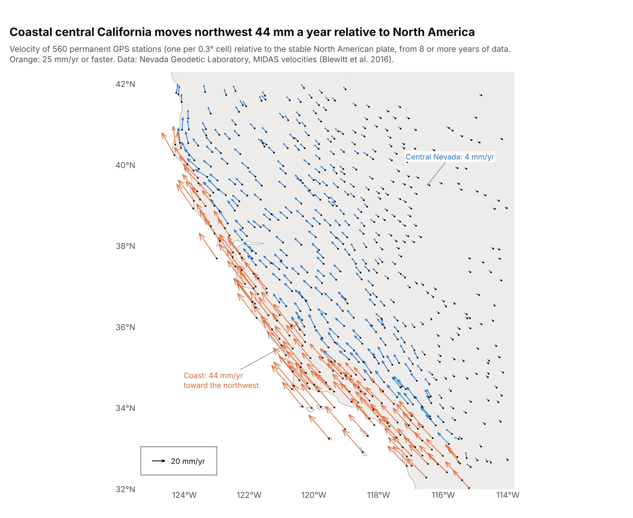
Quiver plot of 560 GPS stations in California and Nevada: orange arrows along the coast point north-west, longest near the shore, blue arrows inland get shorter toward Nevada where they are almost dots, with a 20 mm/yr key

Relative to the stable interior of North America, GPS stations on the central California coast move north-west at a median 44 mm a year, and those in central Nevada at 4. The arrows grow across the boundary between the Pacific and North American plates. Data: Nevada Geodetic Laboratory, MIDAS velocities (Blewitt et al. 2016).

Tip: create_quiver doesn't need a grid, so keep one station per cell of a coarse grid to stop dense networks from turning into a blob.

Get the data from the Nevada Geodetic Laboratory MIDAS GPS velocities in the North America fixed frame
(midas.NA.txt; columns 9 and 10 are east and north velocity in m/yr, 25 and 26 latitude and longitude, 5 the
years of data), stations between 32N and 42N and 125W and 114W with 8 or more years and data since 2020
(columns: station, lat, lon, ve_mm, vn_mm).

Build a plotly quiver plot with ff.create_quiver, one station per 0.3 degree cell, scaleratio = 1/cos(37),
arrows of 25 mm/yr or more in orange and the rest in blue, a 20 mm/yr key and light gray land.

3. Where a compass points

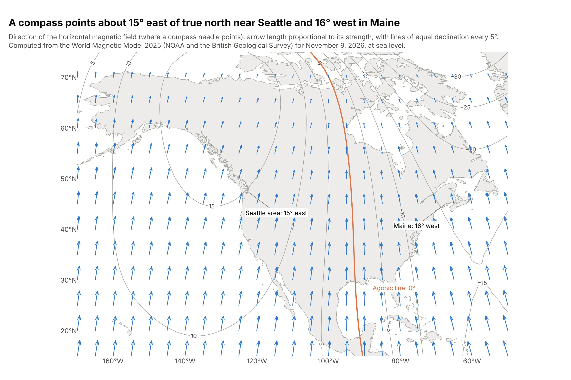
Quiver plot of the horizontal magnetic field over North America with gray lines of equal declination every 5 degrees: arrows tilt right in the west and left in the east, an orange agonic line of zero declination runs from the Arctic down past the Great Lakes to the Gulf of Mexico, and labels mark 15 degrees east near Seattle and 16 degrees west in Maine

A compass needle points along Earth's horizontal magnetic field, which near Seattle is about 15° east of true north and in Maine 16° west. Between them, the agonic line, where the two agree, runs down the middle of the continent. Data: World Magnetic Model 2025 (NOAA and the British Geological Survey), computed for November 9, 2026.

Tip: draw the arrows over contours of the angle you want people to read off (declination here), and highlight the zero line.

Get the data from NOAA NCEI's World Magnetic Model 2025 coefficients (WMM2025.COF), evaluated with pygeomag at
sea level for 2026-11-09 on a 2.5 degree grid from 15N to 75N and 170W to 50W (columns: lat, lon, x_nt, y_nt,
decl_deg).

Build a plotly quiver plot of the horizontal field (u = y_nt, v = x_nt) every 5 degrees with ff.create_quiver and
scaleratio = 1/cos(45), over go.Contour lines of decl_deg every 5 degrees with the 0 line in orange, and label
Seattle and Maine with their declination.

4. Wind at turbine hub height over the North Sea

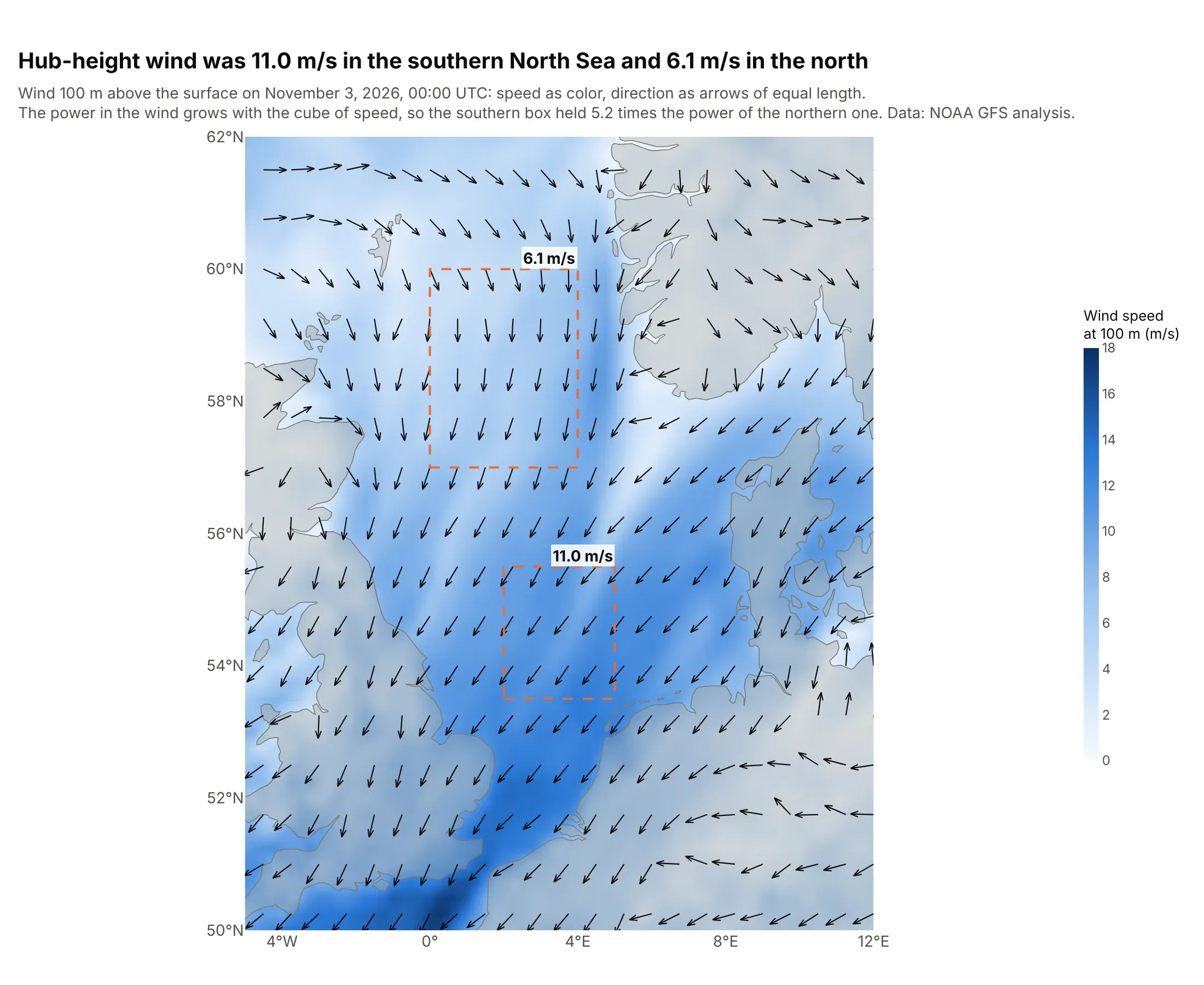
Map of the North Sea on November 3, 2026, colored by wind speed 100 m up, light in the north and dark blue in the south, with black arrows of equal length showing direction and two dashed boxes labeled 6.1 m/s in the north and 11.0 m/s in the south

At 100 m, the height of offshore turbine hubs, the wind averaged 11.0 m/s in the southern box and 6.1 m/s in the northern one. The power in the wind grows with the cube of its speed, so the southern box held 5.2 times as much. Data: NOAA GFS analysis, November 3, 2026, 00:00 UTC.

Tip: when magnitude matters most, put it in color and draw arrows of one length (divide u and v by the speed) for direction only.

Get the data from the NOAA Global Forecast System (GFS) 0.25 degree analysis for 2026-11-03 00 UTC on the NOAA
Open Data Dissemination archive on AWS: UGRD and VGRD at 100 m above ground, 50N to 62N and 5W to 12E
(columns: lat, lon, u, v).

Build a plotly go.Heatmap of wind speed with zsmooth="best" and arrows of equal length every 0.75 degrees from
ff.create_quiver(u/speed, v/speed), scaleratio = 1/cos(56), and dashed boxes with the mean speed of each box.

5. RNA velocity in the developing pancreas

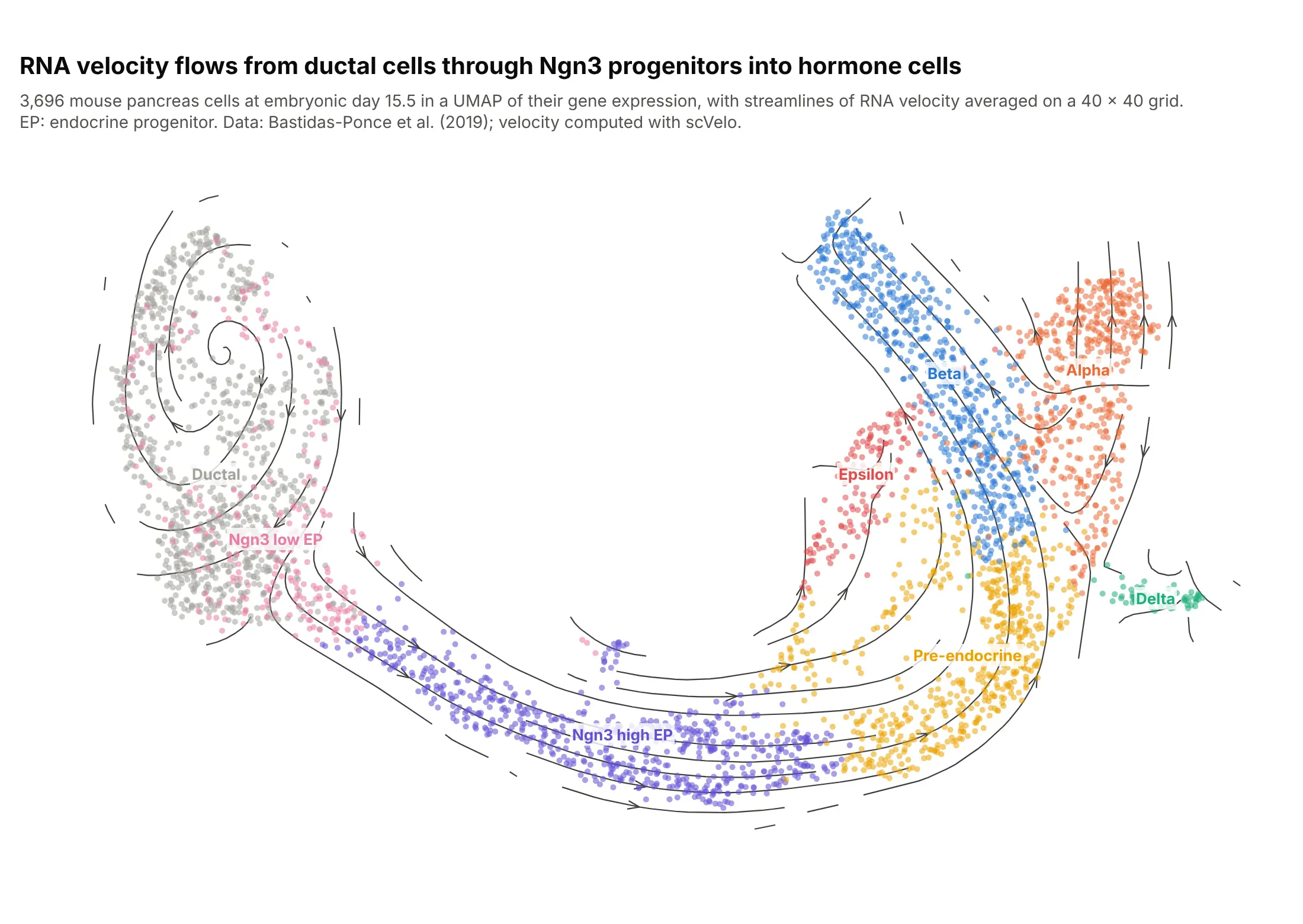
3,696 mouse pancreas cells as colored dots in a UMAP layout, from gray ductal cells on the left through pink and purple Ngn3 progenitors along the bottom to yellow pre-endocrine cells and blue beta, orange alpha, red epsilon and green delta cells on the right, with dark streamlines flowing along that path

RNA velocity estimates which way each cell's gene expression is changing from its ratio of new (unspliced) to mature (spliced) messenger RNA. Averaged on a grid, it flows from ductal cells through neurogenin 3 (Ngn3) progenitors into the hormone-producing alpha, beta, delta and epsilon cells that diabetes research is about. Data: Bastidas-Ponce et al. (2019), 3,696 cells, velocity computed with scVelo.

Tip: average the cell velocities onto a grid for create_streamline, then cut the lines wherever no cell is nearby.

Get the data from the scVelo pancreas data set (Bastidas-Ponce et al. 2019, mouse embryonic day 15.5,
endocrinogenesis_day15.h5ad from the theislab scvelo_notebooks repository), run scVelo's velocity and
velocity_embedding on the UMAP, and average the velocities on a 40 x 40 grid (columns: umap_x, umap_y,
cluster, vx, vy for cells; x, y, u, v for the grid).

Build a plotly scatter of the cells colored by cluster with labels at each cluster's median, and streamlines from
ff.create_streamline over it, cut where no cell is within one grid step.

6. Flow past a spinning cylinder, a computed field

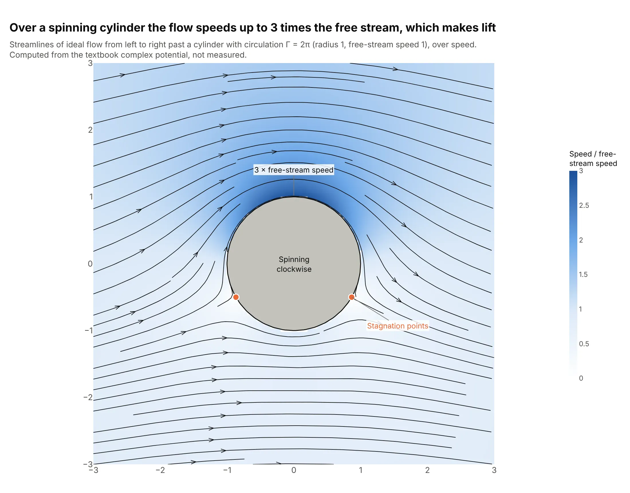
Streamlines of ideal flow from left to right past a gray cylinder over a blue speed map: the lines crowd together over the top, which is dark blue and labeled 3 times free-stream speed, and two orange stagnation points sit on the underside

This is the textbook example of lift, computed from a formula rather than measured. With circulation around the cylinder, the flow over the top speeds up to 3 times the free stream and the two stagnation points move underneath, so pressure is lower on top. Data: computed from the complex potential of ideal flow with circulation (radius 1, free-stream speed 1, circulation 2π).

Tip: for computational fluid dynamics (CFD) results or any analytic field, mask the body and draw it as a filled shape on top of the streamlines.

Compute ideal (potential) flow past a cylinder of radius 1 in a uniform stream of speed 1 with circulation 2*pi on
a 120 x 120 grid from -3 to 3: dw/dz = U(1 - a^2/z^2) + i*Gamma/(2*pi*z), u = Re, v = -Im (columns: x, y, u, v).

Build a plotly figure: a go.Heatmap of speed, ff.create_streamline on top with a tiny placeholder inside the
cylinder, the lines inside it removed, the cylinder as a filled gray circle, and the two stagnation points marked.
Say in the subtitle that the field is computed.