Manhattan Plots - A Complete Guide

TL;DR

• A Manhattan plot shows the result of a genome-wide association study (GWAS): one dot per genetic variant (usually a SNP, a single DNA letter that differs between people), placed along the genome on the x axis, with the strength of the evidence linking it to a trait (−log10 p-value) on the y axis.
• Manhattan plots are also known as GWAS plots or genome-wide significance plots, and are similar to volcano plots, which put the effect size on the x axis instead of the genome position, and Q-Q plots, which check whether the p-values as a whole are inflated.
• Regions linked to the trait rise as towers above a dashed line at p = 5×10⁻⁸, the genome-wide significance threshold, which corrects for about a million independent tests. Height on the chart is the strength of the evidence, not the size of the effect.
• They are the first figure in GWAS of height, type 2 diabetes, cholesterol and COVID-19, and drug developers read them for genes that are already drug targets.
• You can make a Manhattan plot with Plotly in Python from px.scatter or go.Scattergl on a genome-wide x axis, or with Dash Bio's ManhattanPlot.

What is a Manhattan plot?

Manhattan plots look like this:

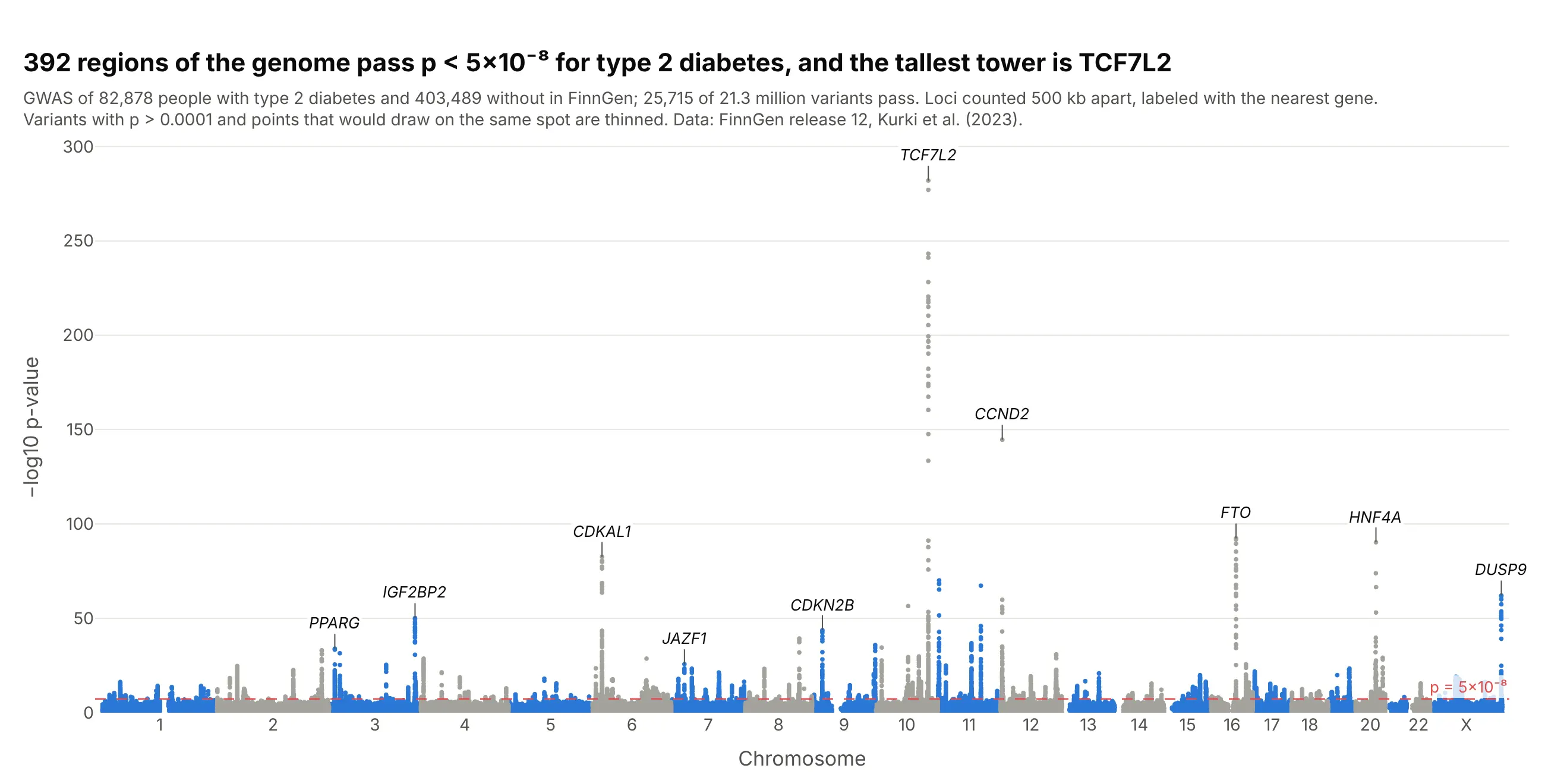
Data: FinnGen release 12, endpoint T2D (Kurki et al. 2023).

How do you read a Manhattan plot? It helps to start with a little of the genetics from high school biology, and with what a p-value measures.

A quick genetics refresher. Your DNA is a sequence of about 3 billion bases, the letters A, C, G and T, packed into 23 pairs of chromosomes (chromosomes 1 to 22, plus X and Y). The whole set is your genome. Genes are stretches of it that hold the instructions for making proteins, and humans have between 20,000 and 25,000 of them. More than 99% of the bases are the same in everyone. Where people do differ, the most common kind of difference is a single-nucleotide polymorphism, or SNP ("snip"): one position where some people have, say, a C and others a T. There are roughly 4 to 5 million of them in each person's genome. "Variant" is the broader word, which also covers small insertions and deletions. SNPs catalogued in NCBI's dbSNP database get a Reference SNP (rs) number such as rs7903146, which is how the variants in this guide are named.

What a GWAS does. A genome-wide association study compares two groups, people with a disease and similar people without it, one variant at a time. For each variant it asks whether one of its letters is more common in the people with the disease than chance would explain. The study behind this chart did that 21.3 million times, for 82,878 people with type 2 diabetes and 403,489 without. A Manhattan plot shows all 21.3 million answers at once, with each variant placed at its position in the genome: chromosome 1 laid end to end with chromosome 2, then 3, and so on to X, about 3 billion bases from left to right.

What the p-value means. Each test gives a p-value: how likely you would be to see a difference between the two groups at least this large if the variant had no real link to the disease. A small p-value means chance alone is a poor explanation. Because the p-values here run from 1 down to 10⁻²⁸², the y axis shows −log10(p), which counts the zeros: 2 means p = 0.01 (1 in 100), 8 means 1 in 100 million, and taller always means stronger evidence. With millions of tests, some variants reach p = 0.0001 by luck alone, so geneticists only count a variant when p is below 5×10⁻⁸ (7.3 on this axis), which is 0.05 divided by the roughly one million independent tests in a European genome. A p-value is not the size of the effect, and it isn't proof that the variant causes the disease (ASA statement on p-values).

With that, these are the takeaways from the chart above:

• Each tower is a region of the genome linked to type 2 diabetes. 25,715 variants pass the 5×10⁻⁸ line, but they cluster into 392 regions, because neighboring variants tend to be inherited together and rise and fall as one tower.
• TCF7L2 on chromosome 10 is the tallest, at −log10 p = 282. It is the gene Grant et al. (2006) first linked to type 2 diabetes. Its lead variant, rs7903146, is carried on 20% of chromosomes in FinnGen, and each copy raises the odds of type 2 diabetes about 1.29 times.
• Hundreds of small effects is the usual picture for a common disease. For the median region, the lead variant changes the odds by about 6% per copy, and three quarters of the 392 change it by less than 10%, so no single variant explains much of anyone's risk.
• The labels are the nearest gene, not a proven cause. A tower says that something in that region is linked to the disease. Finding which variant and which gene is responsible takes follow-up work, such as the zoomed-in regional plot in example 4 below.
• Most of the chart is chance. The dense band at the bottom is what most of the 21 million tests look like: variants with no real link to the disease, whose p-values scatter as chance predicts.

It's often used for charts like these:

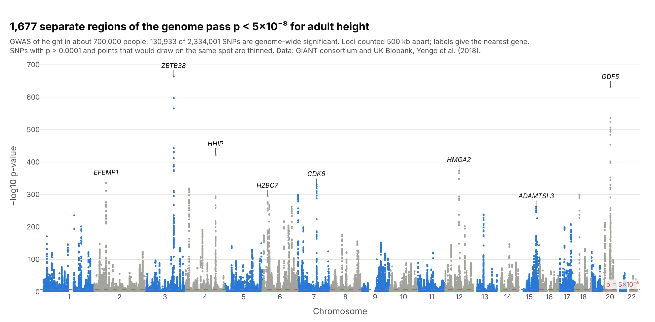
Height, the textbook polygenic trait. In a GWAS of about 700,000 people, 130,933 of 2.3 million SNPs passed p < 5×10⁻⁸, in 1,677 separate regions, so the skyline has towers on almost every chromosome arm. Data: GIANT consortium and UK Biobank, Yengo et al. (2018).

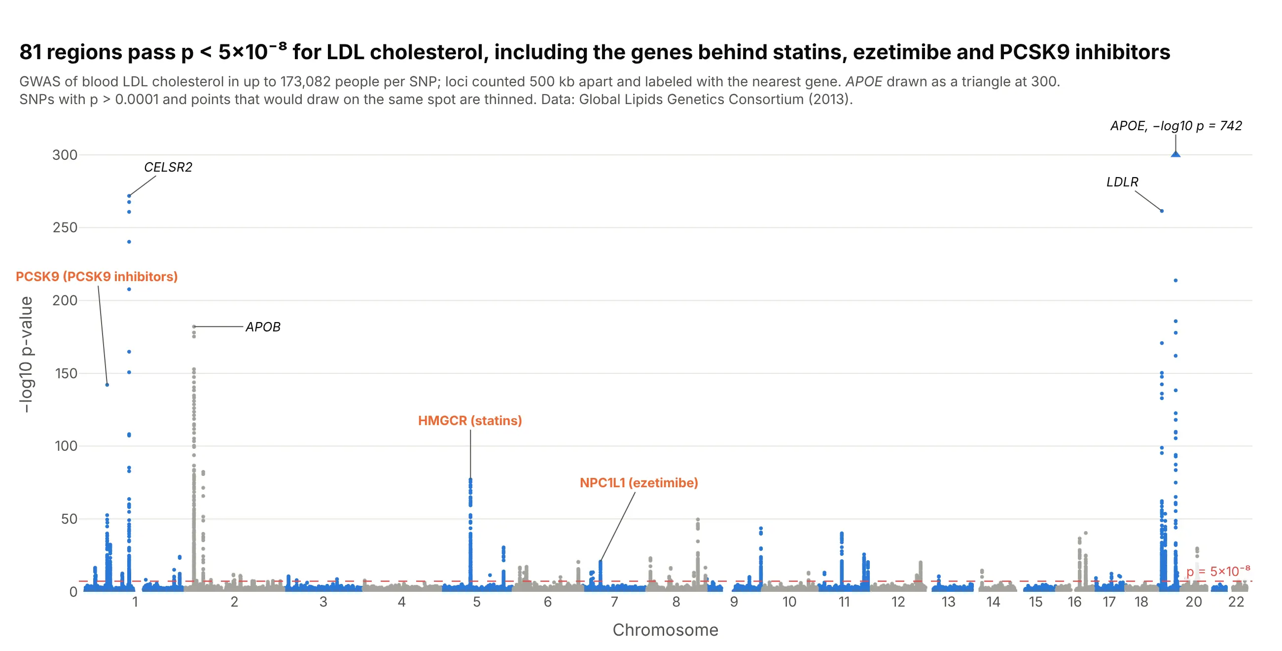
Biomarkers and drug targets. Three of the 81 towers for LDL cholesterol sit on HMGCR, NPC1L1 and PCSK9, the targets of statins, ezetimibe and PCSK9 antibodies, which is why drug developers read these charts for new targets. Data: Global Lipids Genetics Consortium, Willer et al. (2013).

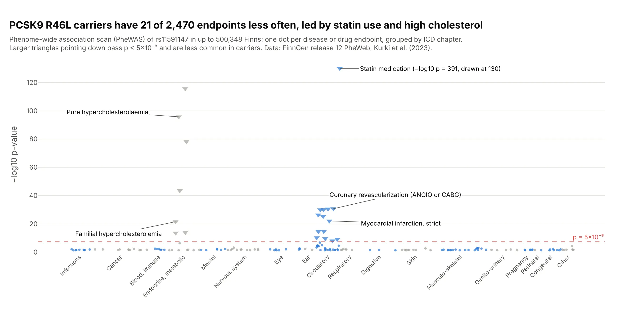
Phenome-wide scans (PheWAS). Turn the chart around and put diseases on the x axis: carriers of the PCSK9 variant R46L had 21 of FinnGen's 2,470 endpoints less often, led by statin use and high cholesterol, and nothing else passed. Data: FinnGen release 12 PheWeb.

A short history

One of the first genome-wide association studies, Klein et al. (2005), tested 116,204 SNPs in 96 people with macular degeneration and 50 without, and its Figure 1 already had the layout: −log10 p "plotted for each SNP in chromosomal order", a dotted line for the Bonferroni cutoff and dotted lines at the chromosome boundaries. As studies grew to millions of variants the chart became the standard first figure of a GWAS, named for its likeness to the Manhattan skyline. The individual data behind that study isn't public, so we haven't redrawn it. The 5×10⁻⁸ line followed from Pe'er et al. (2008), who estimated "a million independent tests genomewide in Europeans" (0.05 divided by a million is 5×10⁻⁸) and twice that number in Africans; some argue it is too strict for replicated borderline signals (Panagiotou and Ioannidis 2012).

Alternatives to a Manhattan plot

Here's the same type 2 diabetes GWAS drawn five ways. Some are better for the question, some worse, some just different:

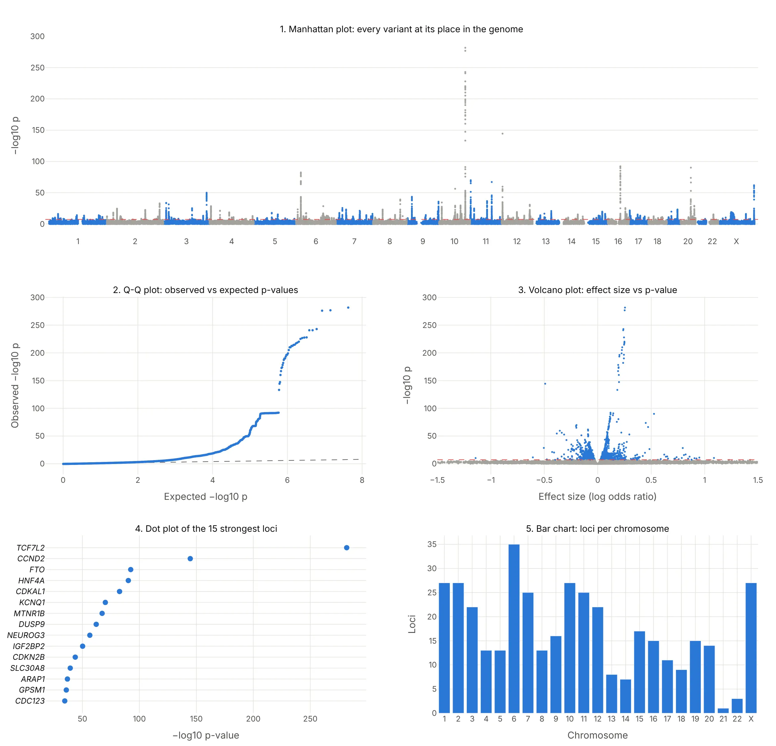
• Q-Q plot (different, and you need both). Observed against expected −log10 p shows whether the p-values as a whole are inflated by population structure or polygenicity, which a Manhattan plot can't show. Papers put it next to the Manhattan plot, as example 6 below does.
• Volcano plot (different, better for effect sizes). Effect size against −log10 p shows which variants matter most per copy, so rare variants with large effects stand out, but the genome position is gone.
• Ranked dot plot of the top loci (better for a slide). The 15 strongest regions with their gene names are easier to read than a skyline, but the other 377 regions and their positions are gone.
• Bar chart of loci per chromosome (worse). It counts regions but hides how strong each one is and where it sits on the chromosome.
• Regional plot (works too, for one tower). Zooming into one region shows which genes the signal sits on, as example 4 below does, but you need the genome-wide view first to know where to zoom.

How to make a Manhattan plot

With AI

ChatGPT, Claude Code, GitHub Copilot, Cursor and other AI tools are excellent at writing Plotly code. Name Plotly in the prompt, and say how big the file is so the code thins the points:

With Plotly Studio

Plotly Studio is a desktop app where you point an AI at a dataset and it builds charts and a Dash app around your questions. Ask for a Manhattan plot the same way:

Show a Manhattan plot of the GWAS results with chromosomes in alternating colors, a dashed line at p = 5×10⁻⁸, the top 10 loci labeled with their genes, a Q-Q plot next to it, and a dropdown to zoom into one chromosome.

Make a Manhattan plot in Python or JavaScript

This is the code AI tools write under the hood. Plotly doesn't need a special trace for a Manhattan plot: it's px.scatter on a genome-wide x axis, where each chromosome's positions are shifted by the total length of the chromosomes before it.

To label the top loci, pick the strongest SNP in each region and add an annotation with fig.add_annotation(x=..., y=..., text="<i>TCF7L2</i>", ax=0, ay=-22). If a p-value in your file is 0 because it underflowed, compute −log10 p from the z-score (beta divided by its standard error) instead, as the examples here do. The Plotly scatter plot documentation covers hover text and styling.

In JavaScript, plotly.js draws the same thing from a scatter trace, chromosome offsets and a line shape:

Make a Manhattan plot with Dash Bio

Dash Bio is Plotly's open-source library of bioinformatics charts for Dash, and its ManhattanPlot builds the figure from a DataFrame with CHR, BP, P, SNP and GENE columns (X renumbered as 23), highlighting the points above the line. Both lines are given on the −log10 scale: genomewideline_value defaults to −log10(5×10⁻⁸) and suggestiveline_value to 8, so set the suggestive line yourself:

Check two things in dash-bio 1.0.2, the current release when we tested it. It ran with NumPy 1.26 but raised TypeError: %i format: a real number is required, not numpy.ndarray with NumPy 2.5, and with NumPy 1.26 the hover names were wrong on every chromosome after the first, because each chromosome's trace gets the hover text of the whole DataFrame. Until that's fixed, the px.scatter version above is the safer choice for a figure people will hover over. In a Dash app, put either figure in a dcc.Graph and connect a dcc.Slider to the threshold, as the Dash Bio example does.

Share it

Every Plotly chart has a Share chart button (the cloud icon in its toolbar) that uploads it to Plotly Cloud and gives you a link. Only you can see it until you change its visibility.

For a live app, put the chart in a Dash app and publish it with the Plotly Cloud CLI. Coding agents can run these commands for you:

If your data has to stay in your own cloud or data center, publish to Dash Enterprise instead.

Dos and don'ts

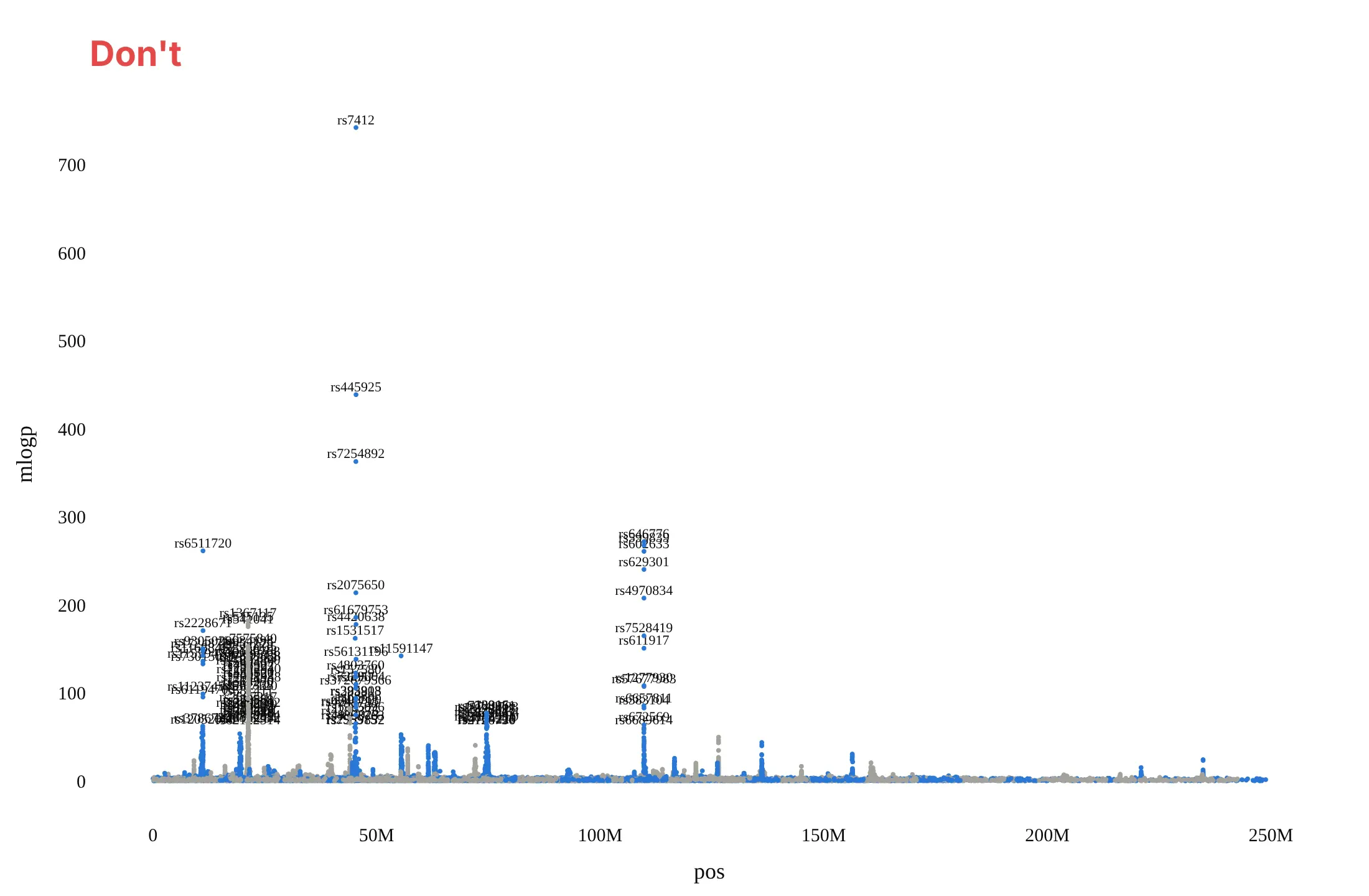
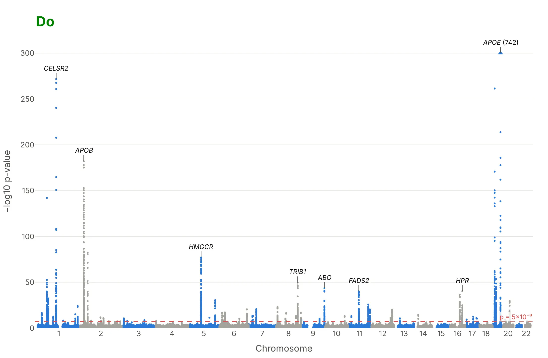
Most of the work in a published Manhattan plot is the x axis, the threshold and the labels. Here is the LDL cholesterol GWAS both ways, in the same colors.

Don't plot each variant's position within its chromosome as x, which draws all 22 chromosomes on top of each other, leave out the significance line, label every SNP above a cutoff so the rs numbers pile up, or use a default serif font and raw column names as axis titles:

Do shift each chromosome by the ones before it and label the chromosome numbers, alternate two colors by chromosome, draw the 5×10⁻⁸ line with its value, label a handful of towers with gene names, and cap a tower that would flatten the rest, with its real value:

Checklist

Do

• Put the genome position on x (chromosome offsets added) and −log10 p on y, and label the chromosomes, not the base pairs.
• Draw the genome-wide line at 5×10⁻⁸ and write its value; add a suggestive line (often 10⁻⁵) only if the text uses it.
• Label the strongest variant of the top 5 to 15 regions with its nearest gene, in italics, and keep every name in the hover text.
• Say in the subtitle how many people and variants were tested, and how the points were thinned.
• Use WebGL (render_mode="webgl" or go.Scattergl) and thin the variants with p > 10⁻⁴; they only form the floor.
• Show a Q-Q plot next to it.

Don't

• Read the height of a tower as the size of the effect; a common variant with a small effect can be taller than a rare one with a large effect.
• Call each dot above the line a separate finding; neighboring variants are inherited together and form one tower.
• Let one tower set the y axis for the whole chart; cap it and write its value.

Options to customize

A Manhattan plot in Plotly is a scatter trace on a genome-wide x axis plus lines and annotations, so these are the options that matter most. The full lists are in the px.scatter reference and the scattergl trace reference.

1. x, y: the cumulative genome position (position plus the chromosome's offset) and −log10 p, computed as columns first.
2. xaxis.tickvals, xaxis.ticktext: one tick at the middle of each chromosome, labeled 1 to 22 and X.
3. color with color_discrete_sequence, or marker.color as an array: two alternating colors by chromosome.
4. render_mode="webgl" or go.Scattergl: WebGL markers, which you need above about 20,000 points.
5. add_hline with line_dash="dash" and annotation_text: the 5×10⁻⁸ line and a suggestive line.
6. add_annotation with ax, ay: gene labels with leader lines on the top loci.
7. hover_name, hover_data, hovertemplate: rsID, chromosome, position, p-value and gene on hover.
8. marker.symbol: triangles for points capped at the top of the axis.
9. yaxis.range: a cap, so one huge tower doesn't flatten the others.
10. make_subplots(shared_xaxes=True): stacked Manhattan plots of several traits, or a regional plot with a gene track below it.
11. Negative y values with yaxis.tickvals and positive ticktext: a Miami plot, two traits mirrored around the x axis.
12. dash_bio.ManhattanPlot(genomewideline_value=..., suggestiveline_value=..., highlight_color=...): the same chart from a DataFrame in one call.

More Manhattan plot examples

Six more Manhattan plots built from real public data, each with its source, the technique that makes it work and a prompt to rebuild it.

1. Alzheimer's disease, where one tower dwarfs the rest

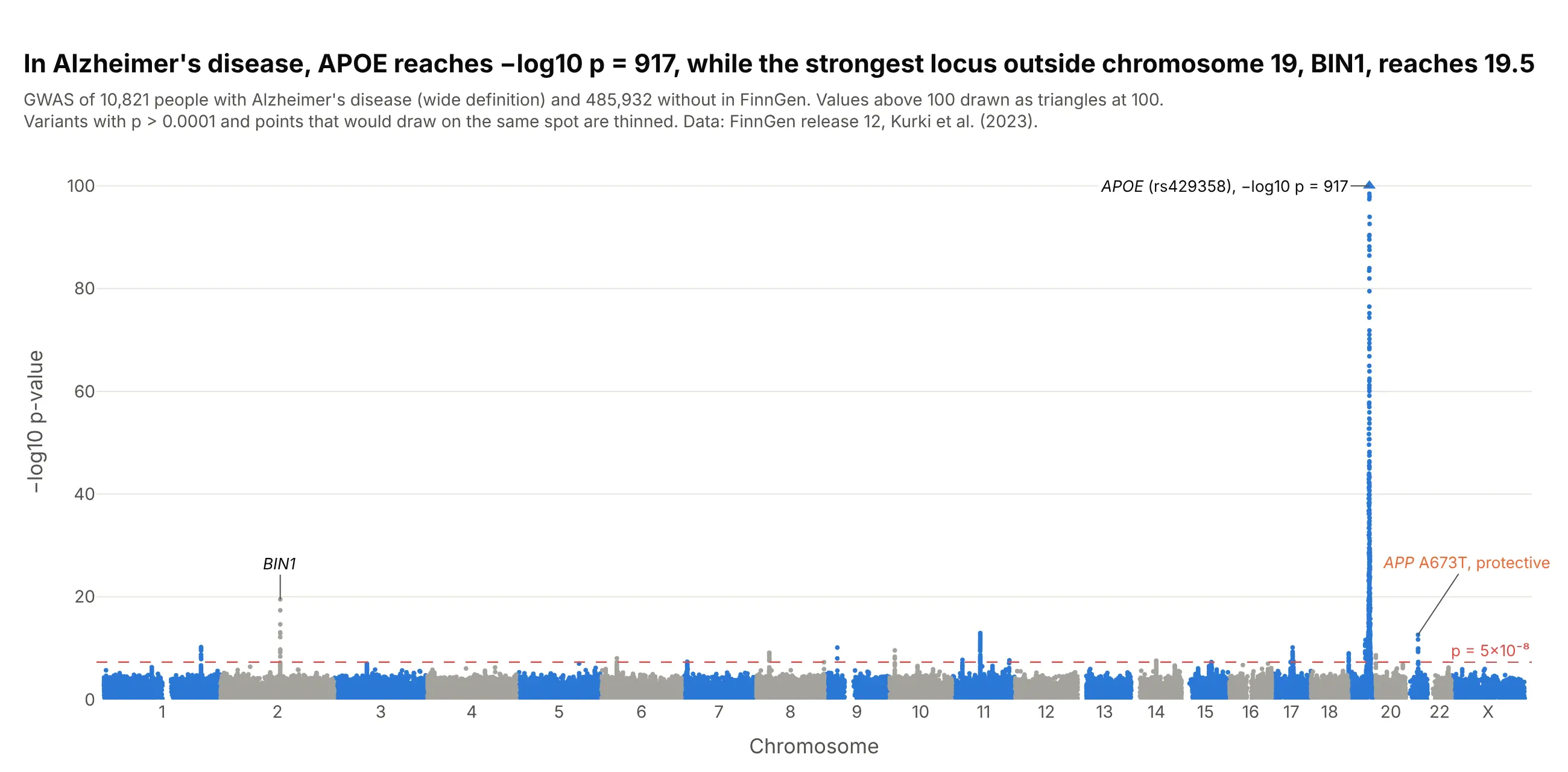
APOE reaches −log10 p = 917 for Alzheimer's disease in FinnGen, while the strongest region outside chromosome 19, BIN1, reaches 19.5. The rare APP variant A673T, which Jonsson et al. (2012) found to protect against the disease, passes too. Data: FinnGen release 12, endpoint G6_AD_WIDE (10,821 cases, 485,932 controls).

Tip: cap the y axis and draw the capped variants as triangles with the real value written next to them, or every other tower disappears into the floor.

2. Critical COVID-19 in the Host Genetics Initiative

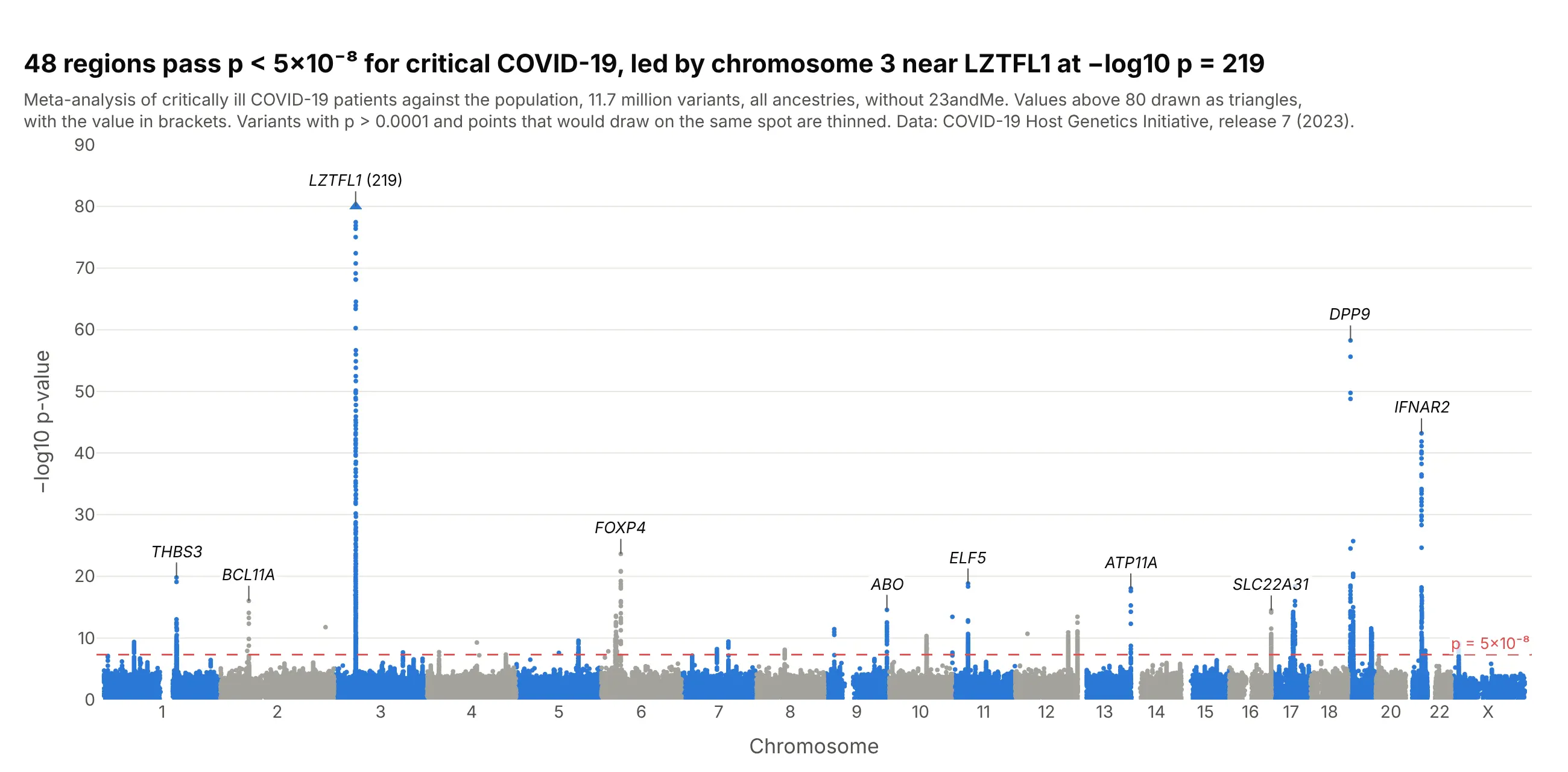
Of 48 regions linked to critical COVID-19, the chromosome 3 region near LZTFL1 is the strongest at −log10 p = 219, and smaller towers sit on interferon and immune genes such as IFNAR2, TYK2 and OAS1. Data: COVID-19 Host Genetics Initiative, release 7 (2023), critical illness against the population.

Tip: for a disease with a few strong loci, label more towers than you would for height, because each one is a candidate for follow-up.

3. A Miami plot of LDL and HDL cholesterol

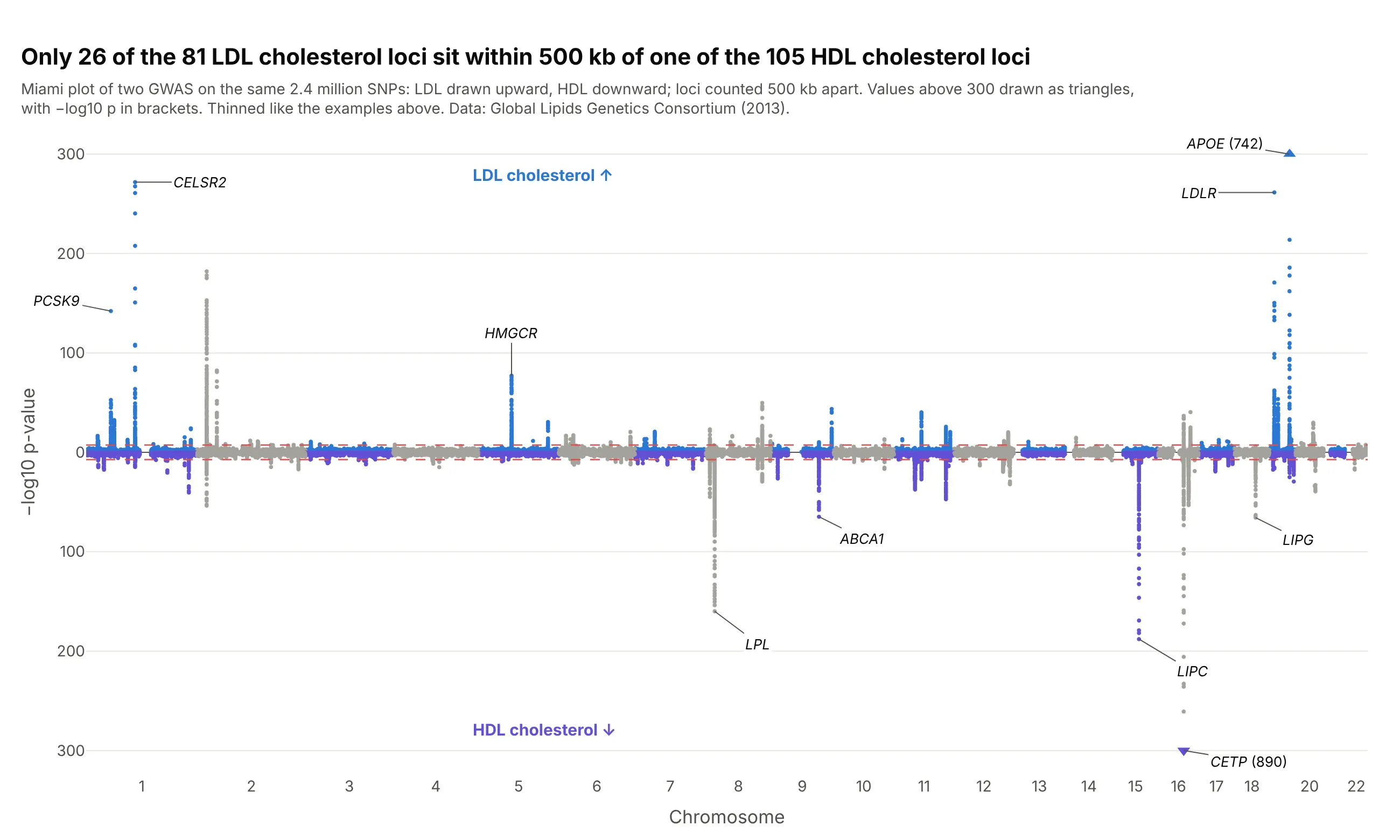
Mirroring two Manhattan plots around one genome axis shows which towers two traits share. Only 26 of the 81 LDL cholesterol regions sit within 500 kb of one of the 105 HDL regions, and CETP, the tallest for HDL at 890, is a small tower for LDL. Data: Global Lipids Genetics Consortium (2013).

Tip: draw the second trait with negative y values and relabel the ticks as positive numbers, so both halves read as −log10 p.

4. Zooming into one tower: the TCF7L2 region

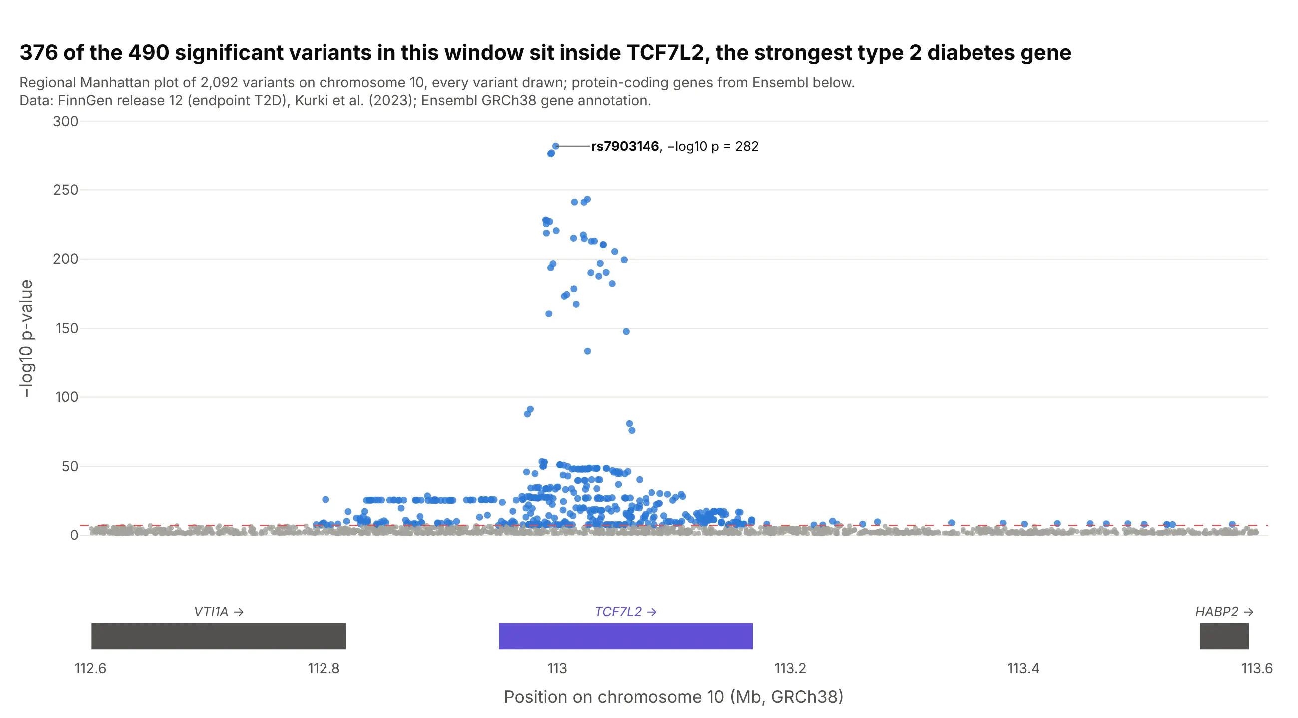
The genome-wide view says a region matters; the regional view shows which gene it sits on. 376 of the 490 significant variants in this 1 Mb window are inside TCF7L2, and every variant above −log10 p = 100 is. Data: FinnGen release 12, endpoint T2D, every variant in the window; genes from Ensembl.

Tip: put the gene track in a second row with make_subplots(shared_xaxes=True), so zooming moves both. Tools like LocusZoom also color each variant by its correlation with the lead variant.

5. Three diseases stacked on one genome axis

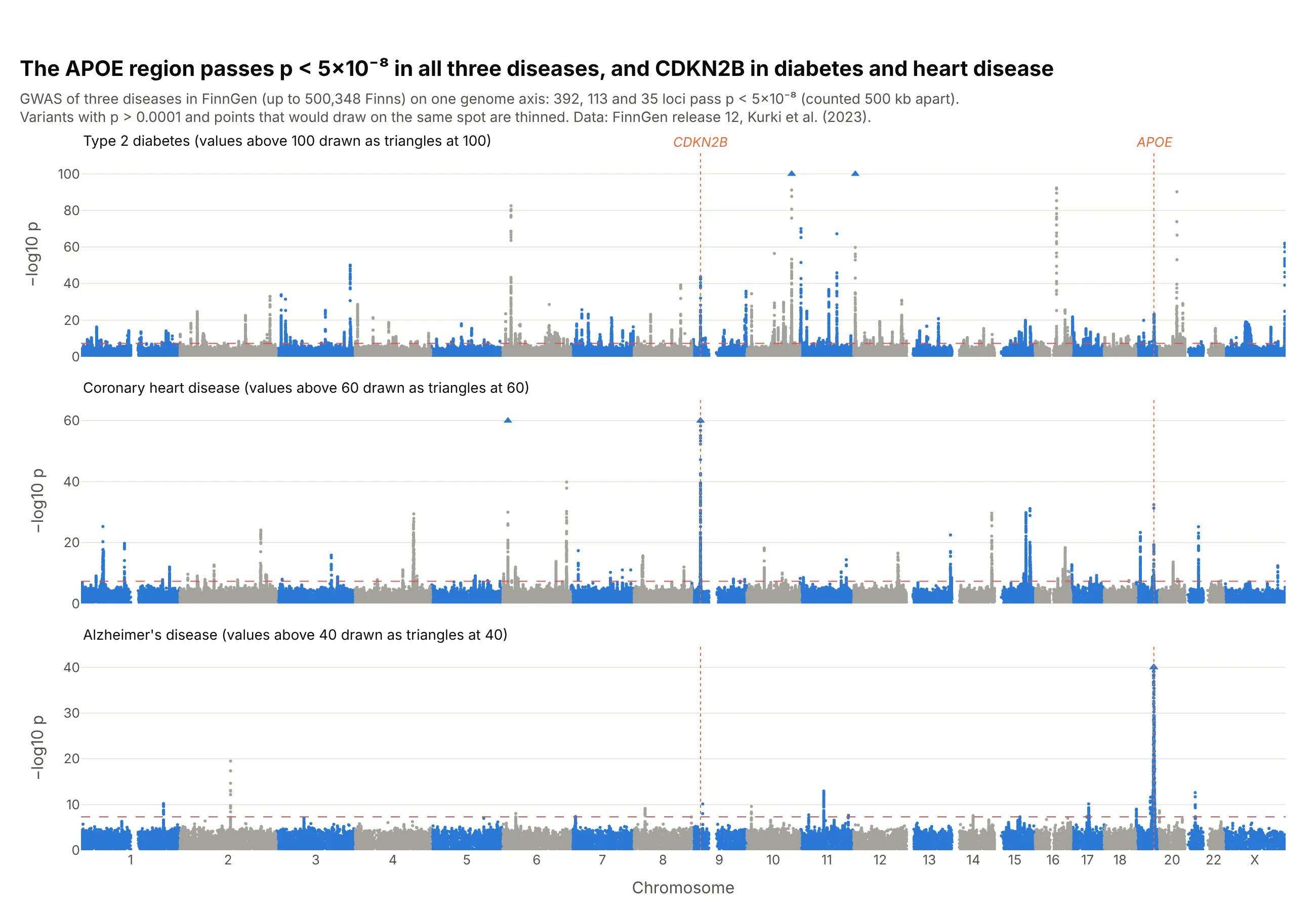
Stacking GWAS from the same biobank on one axis shows where diseases share biology: the APOE region passes in type 2 diabetes, coronary heart disease and Alzheimer's disease, and CDKN2B on chromosome 9, the strongest heart disease region at 155, also passes for diabetes. Data: FinnGen release 12, endpoints T2D, I9_CHD and G6_AD_WIDE.

Tip: give each panel its own capped y axis, and say in the panel title where the cap is.

6. A Q-Q plot next to the Manhattan plot

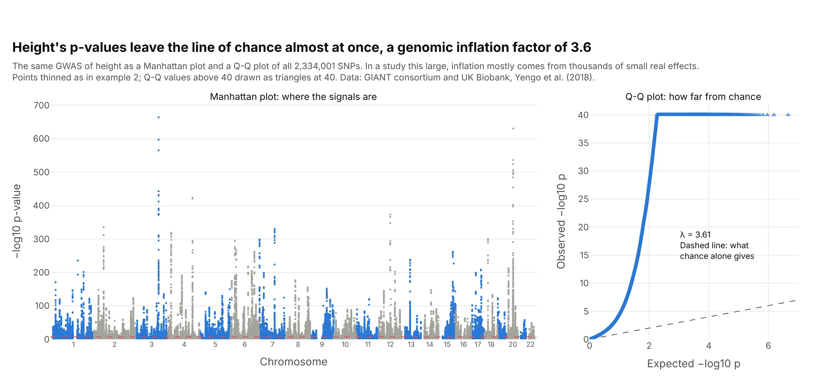
The Q-Q plot answers what the Manhattan plot can't: are the p-values as a whole higher than chance? For height the genomic inflation factor is 3.6, which in a study of about 700,000 people mostly reflects thousands of small real effects (Yang et al. 2011); LD score regression separates that from confounding (Bulik-Sullivan et al. 2015). Data: GIANT consortium and UK Biobank, Yengo et al. (2018).

Tip: compute the Q-Q points from every variant before you thin the Manhattan plot, then keep a few thousand evenly spaced ranks plus the top 1,000.