Polar Charts - A Complete Guide

TL;DR

• A polar chart places each value by an angle around a circle and a distance from the center, so it suits data that is a direction (wind, the sun's position) or a cycle (hours of the day, months, days of the year).
• Polar charts are also known as polar plots and polar graphs, and the bar version as a polar area diagram, coxcomb chart or Nightingale rose. They are similar to radar charts and wind roses, which are both polar charts with a special job.
• There are three main kinds: polar scatter charts (one dot per observation), polar line charts (a closed loop per series or year) and polar bar charts (one wedge per angle bin, which becomes a polar area chart when the wedges' area carries the value).
• You can make each one with Plotly in one line of code: px.scatter_polar, px.line_polar and px.bar_polar in Python, or the scatterpolar and barpolar traces in JavaScript.
• Set the start angle and direction yourself (rotation=90, direction="clockwise") for clocks, calendars and compasses, because Plotly's default puts 0 at three o'clock and runs counterclockwise, the convention of mathematics.

What is a polar chart?

Polar charts look like this:

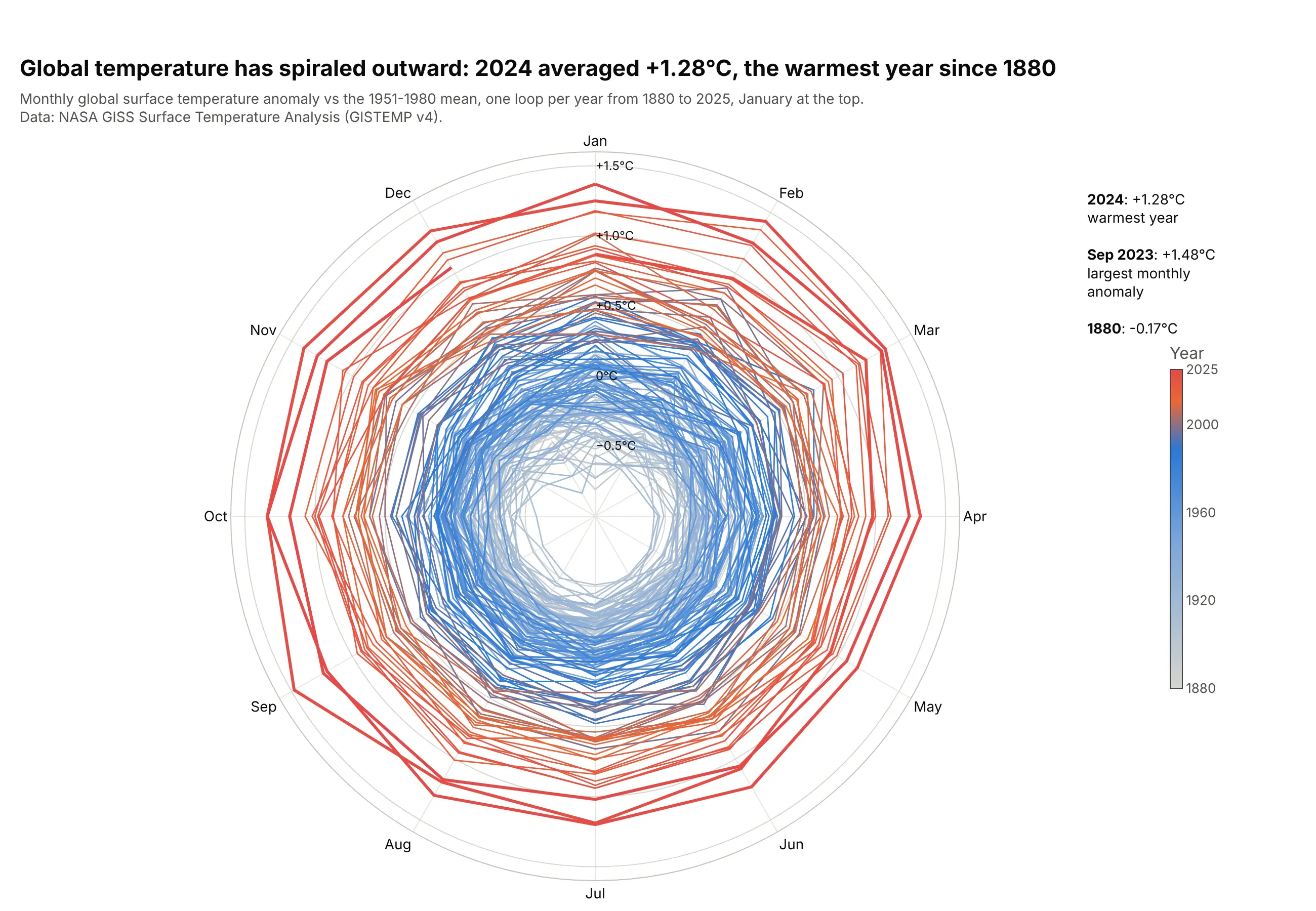
Data: NASA GISS Surface Temperature Analysis (GISTEMP v4).

How do you read a polar chart? In the example above, notice these things:

• The angle is the month, starting with January at the top and running clockwise like a clock, so each year is one loop around the circle and December joins the next January.
• The distance from the center is the temperature anomaly against the 1951-1980 average, read off the labeled rings. The axis starts at -1 °C, so months colder than that average sit inside the 0 °C ring, as 94% of the months from 1880 to 1939 do.
• Color shows the year, from gray in the 1880s to red in the 2020s. Only 3 months since 1980 fall inside the 0 °C ring, the last in September 1992.
• The outermost loops are the most recent years. Every month of 2024 and 2025 was at least 1.0 °C above the average, 2024 averaged +1.28 °C, and September 2023 has the largest anomaly in the record at +1.48 °C.

It's often used for charts like these:

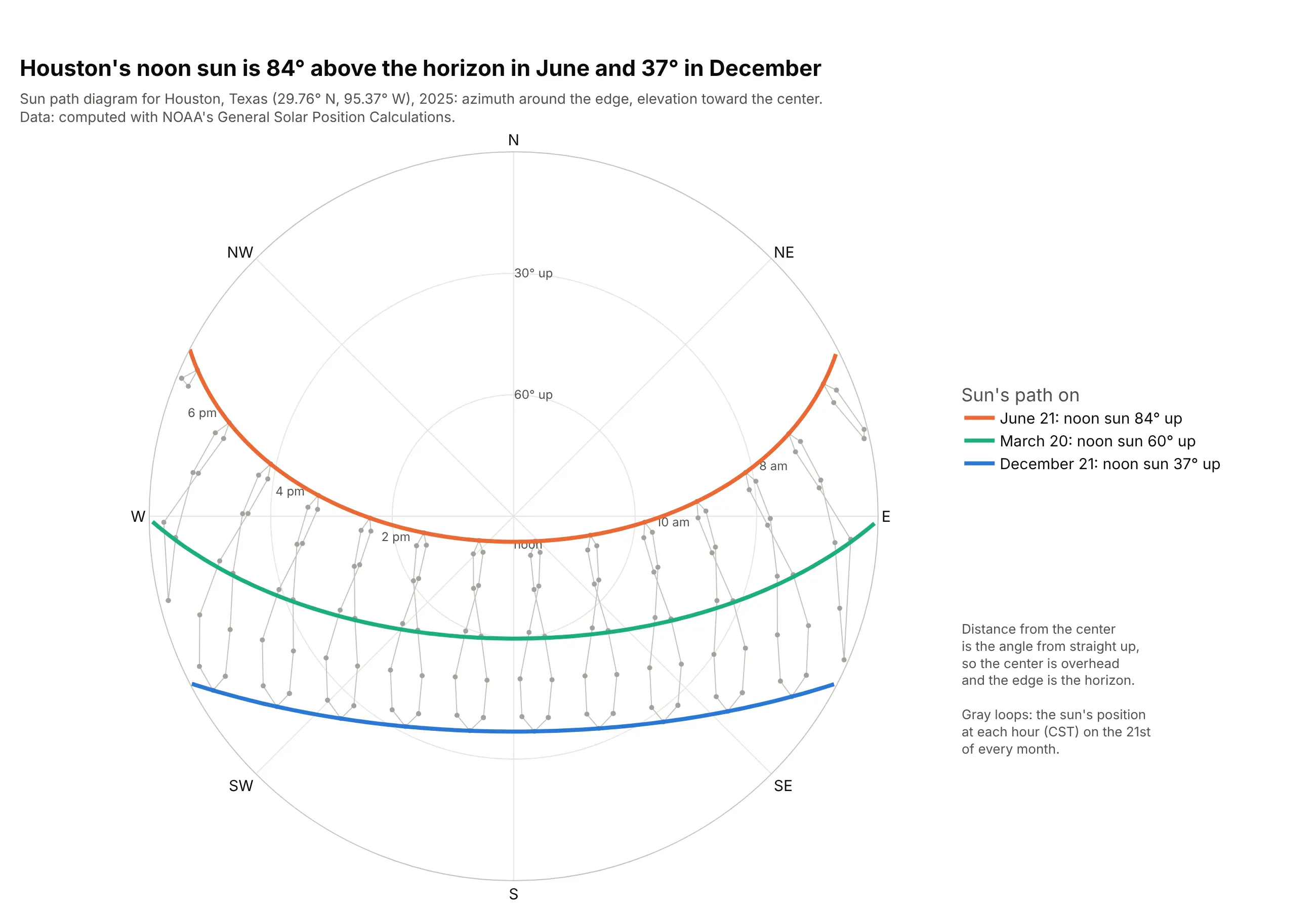
Sun path diagrams. In Houston, the noon sun is 84° above the horizon on June 21 and 37° on December 21, the angles a solar designer reads off this chart before placing panels or shading. Data: computed with NOAA's General Solar Position Calculations.

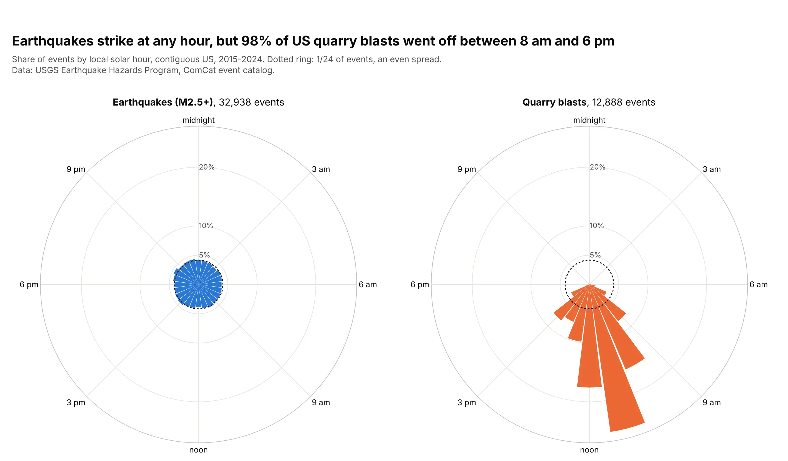
Hours of the day. 98% of 12,888 US quarry blasts from 2015 to 2024 went off between 8 am and 6 pm, while earthquakes spread evenly around the clock. Data: USGS Earthquake Hazards Program, ComCat event catalog.

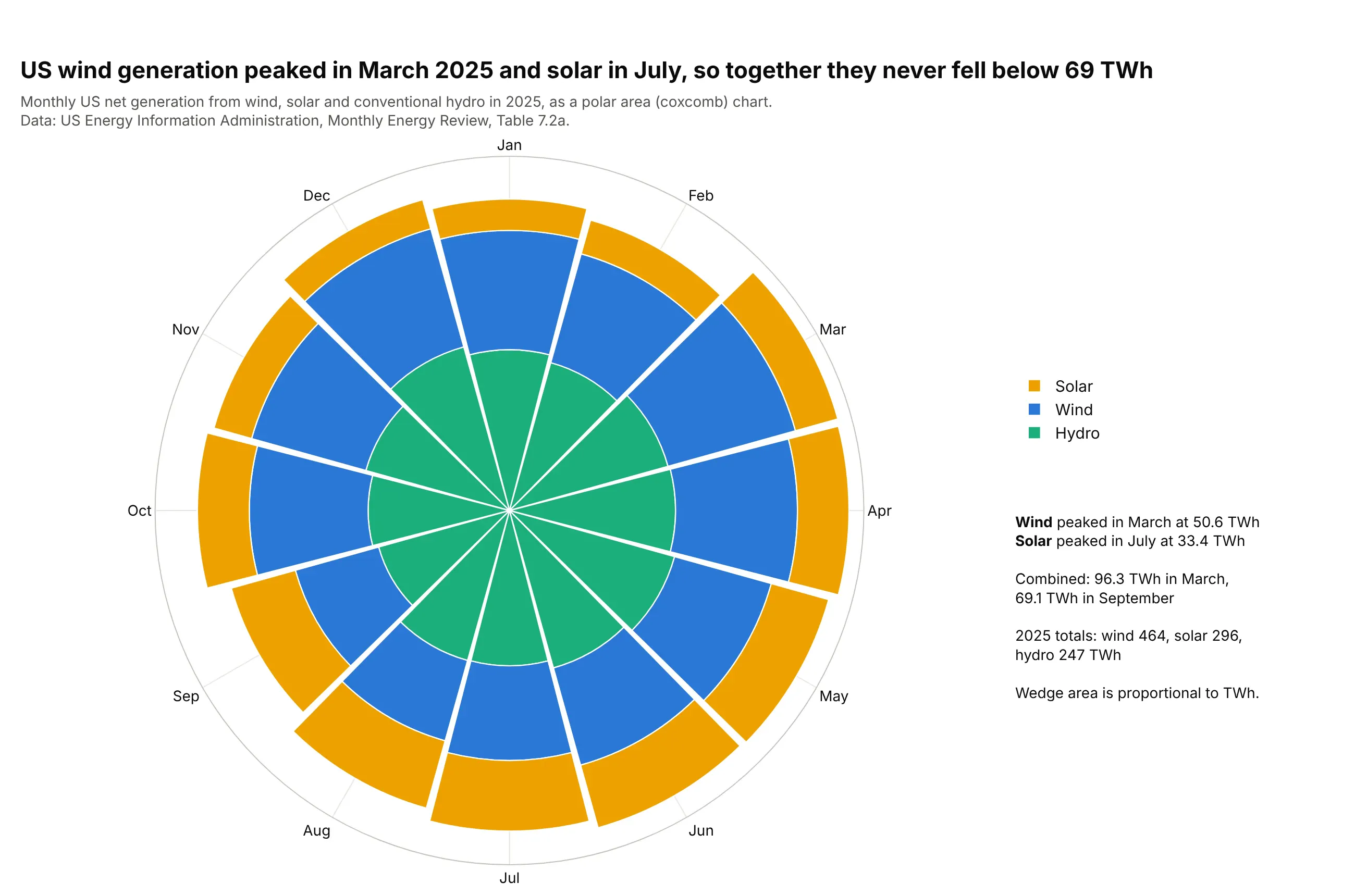
Months of the year, as a polar area chart. US wind generation peaked in March 2025 at 50.6 TWh and solar in July at 33.4 TWh, so the three sources together never fell below 69 TWh in a month. Data: US Energy Information Administration, Monthly Energy Review, Table 7.2a.

Types of polar charts

Plotly draws all of these on the same polar axes, an angular axis around the edge and a radial axis from the center out, so you can mix them in one chart.

Polar scatter chart

A polar scatter chart puts one marker per observation at its angle and distance, as in the sun path diagram above and the buoy winds in example 3 below. In Python it's px.scatter_polar, and for more than about 50,000 points use render_mode="webgl" (the scatterpolargl trace).

Polar line chart

A polar line chart joins the points of each series in order, which makes a closed loop for anything that repeats, like the months in the climate spiral. In Python it's px.line_polar with line_group for one loop per year, or line_close=True to join the last point to the first. A radar chart is a polar line chart whose angles are different measures instead of one continuous variable.

Polar bar chart

A polar bar chart (px.bar_polar, the barpolar trace) draws one wedge per angle bin, with its length as the value. The quarry blast chart is a polar histogram of hours, and a wind rose is a stacked polar bar chart of how often the wind blows from each direction at each speed.

Polar area chart (Nightingale rose or coxcomb)

A polar area chart is a polar bar chart with equal angles where each wedge's area, not its length, is proportional to the value. Area grows with the square of the radius, so you set each radius to the square root of the value, as Florence Nightingale did and as the renewables chart above does. The dos and don'ts below show the difference on the same data.

A short history

Wikipedia's history of the pie chart credits André-Michel Guerry with the first known polar area diagrams, which he called "courbes circulaires" (circular curves), in an 1829 paper on wind direction and on births and deaths by hour of the day, and Léon Lalanne with a polar diagram of wind directions in 1843. The best known is Florence Nightingale's 1858 diagram of deaths in the British Army during the Crimean War, which showed that preventable disease killed far more soldiers than wounds did; Lee Brasseur analyzes it in Technical Communication Quarterly (2005). Here it is redrawn from her data, with each wedge's area equal to the death rate:

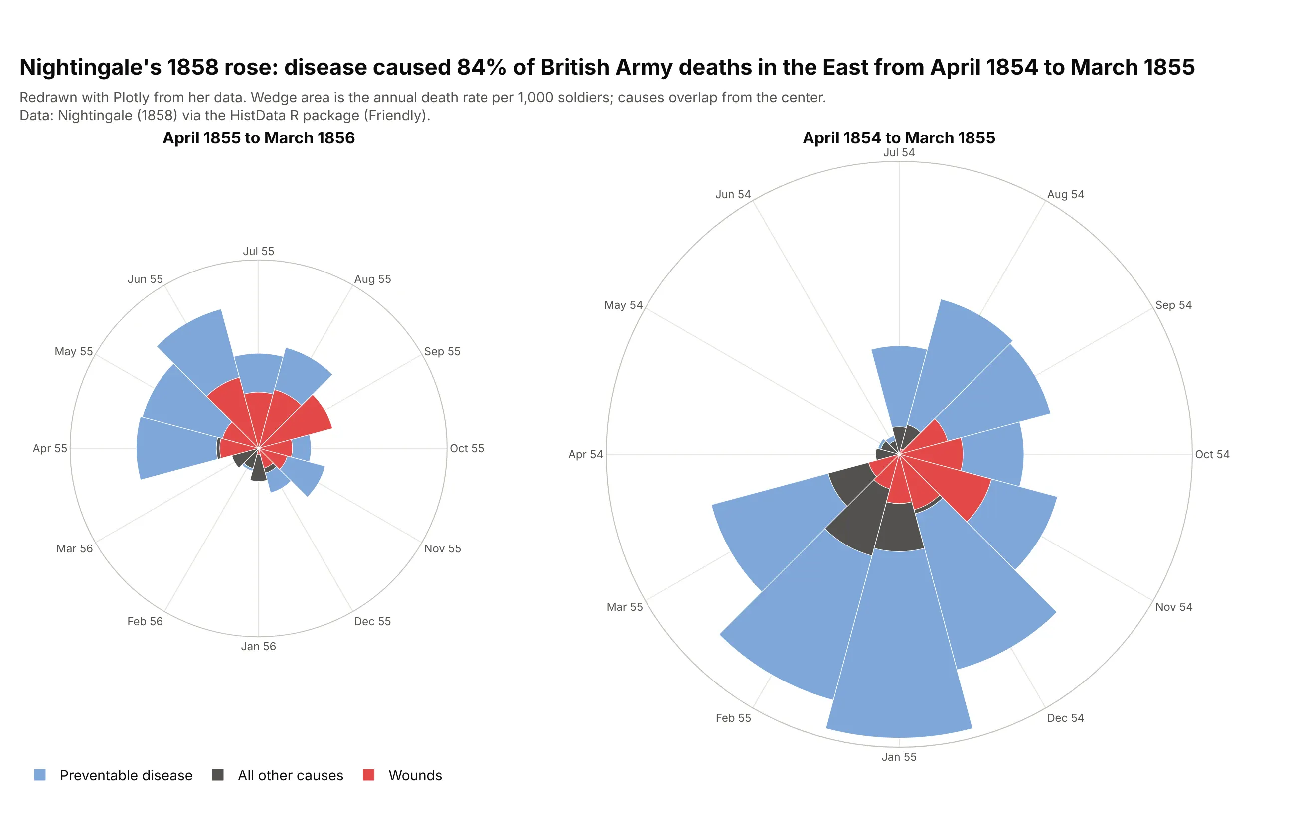
Data: Nightingale (1858) via the HistData R package. In the first year, disease caused 84% of the deaths, and its annual rate peaked at 1,023 per 1,000 soldiers in January 1855.

A recent classic is Ed Hawkins' climate spiral of 2016, a polar line chart of monthly global temperatures that the main example above redraws with NASA's data.

Alternatives to a polar chart

Here's the same 146 years of monthly temperatures drawn six ways. Some are better for the question, some worse, some just different:

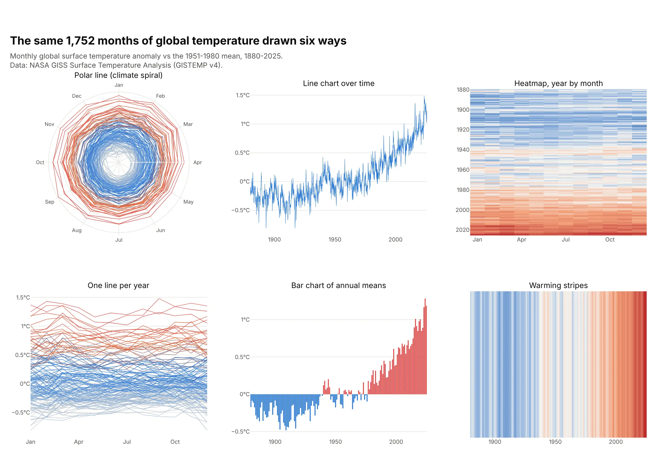
• Polar line chart (works for cycles and for impact). It shows the seasonal loop and the drift outward at once, but reading an exact value or the gap between two years is harder than on straight axes.
• Line chart over time (better for the trend). One line from 1880 to 2025 shows the long rise and the month-to-month noise most precisely, and it's what most readers expect.
• Heatmap of year by month (works too). Every month gets its own cell, so you can find a single month, though colors are harder to compare than positions.
• One line per year on straight axes (worse here). It is the same chart as the spiral unrolled, but December and January end up at opposite edges, and 146 lines tangle into a band.
• Bar chart of annual means (better for comparing years). The years line up on one baseline, so 2024 is plainly the tallest bar, but the months and the seasonal cycle are gone.
• Warming stripes (different). One colored stripe per year has no axis at all, which makes it a poster rather than a chart you read numbers from.

When the angle is a direction instead of a time, as in a wind rose or a sun path diagram, a polar chart is the natural choice, because a compass is already a circle.

How to make a polar chart

With AI

ChatGPT, Claude Code, GitHub Copilot, Cursor and other AI tools are excellent at writing Plotly code. Name Plotly in the prompt, and say where the circle starts, which way it runs and what the radial axis should cover:

With Plotly Studio

Plotly Studio is a desktop app where you point an AI at a dataset and it builds charts and a Dash app around your questions. Ask for a polar chart the same way:

Show a polar bar chart of quarry blasts by hour of the day, midnight at the top and clockwise like a clock, each bar the share of all blasts in that hour, with earthquakes as a second chart for comparison.

Make a polar chart in Python

This is the code AI tools write under the hood. Plotly Express makes each kind of polar chart in one line of code, and the Plotly polar chart documentation and bar polar documentation cover the rest:

Numbers in theta are read as degrees, and text is read as categories spaced evenly around the circle in the order they first appear. render_mode="svg" in the first chart keeps px.line_polar from switching to WebGL above 1,000 rows. With go.Scatterpolar and go.Barpolar from plotly.graph_objects you get the same traces with full control, which is how the examples in this guide are built.

Make a polar chart in JavaScript

In JavaScript, plotly.js draws polar charts with the scatterpolar and barpolar traces. This page makes a polar area chart, where each wedge's area is proportional to the value, and a polar line chart of the same data:

For a plain polar bar chart, where the length is the value, pass the values as r and leave out base. The plotly.js polar chart documentation has more examples.

Share it

Every Plotly chart has a Share chart button (the cloud icon in its toolbar) that uploads it to Plotly Cloud and gives you a link. Only you can see it until you change its visibility.

For a live app, put the chart in a Dash app and publish it with the Plotly Cloud CLI. Coding agents can run these commands for you:

If your data has to stay in your own cloud or data center, publish to Dash Enterprise instead.

Dos and don'ts

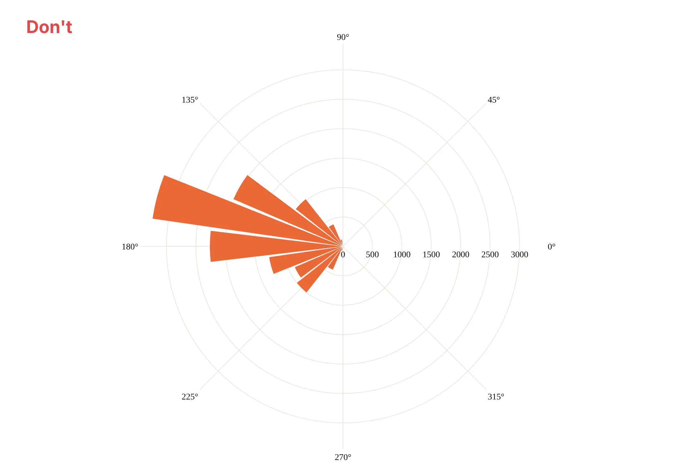
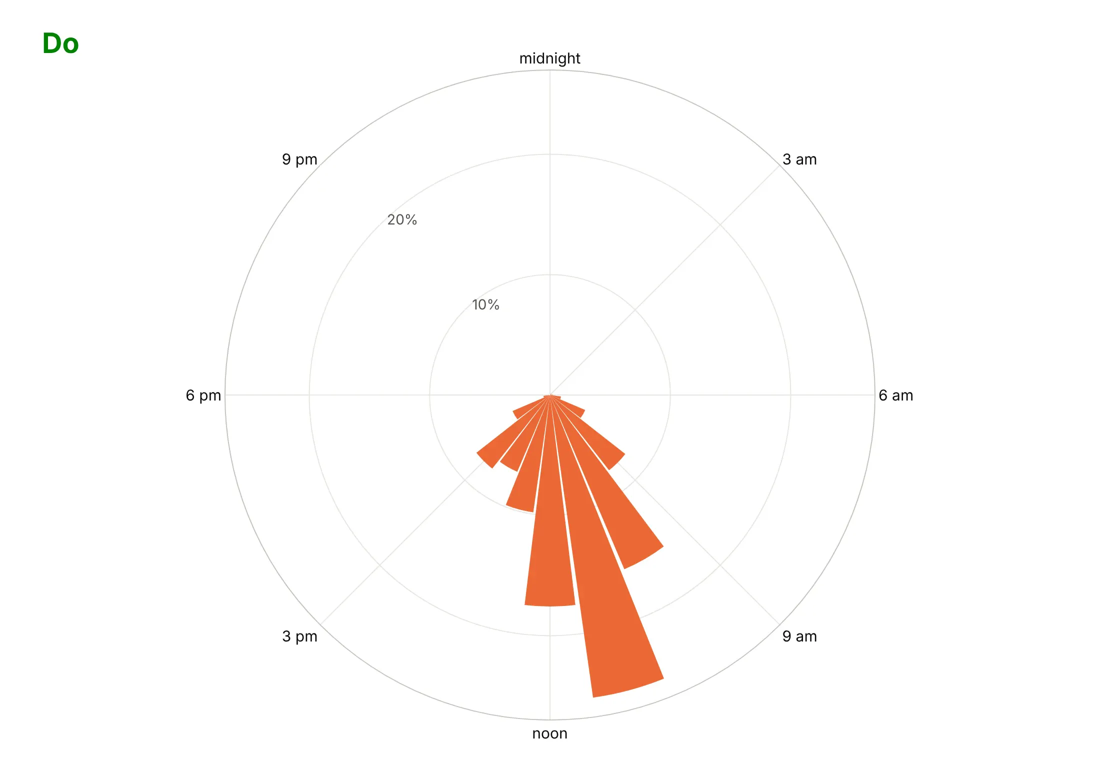
Most mistakes in a published polar chart come from the angular axis, because readers expect a clock or a compass and Plotly starts from mathematics. Here are the 12,888 quarry blasts both ways, in the same color.

Don't pass hours as degrees (hour × 15) and keep the default orientation, which puts midnight at three o'clock and runs the day counterclockwise, label the angles in degrees instead of times, print raw counts on radial ticks that sit over the bars, or use a default serif font:

Do put midnight at the top and run clockwise like a clock, label the hours, show each hour's share in percent, and move the radial tick labels to an empty part of the circle:

Make area match the value in a polar area chart

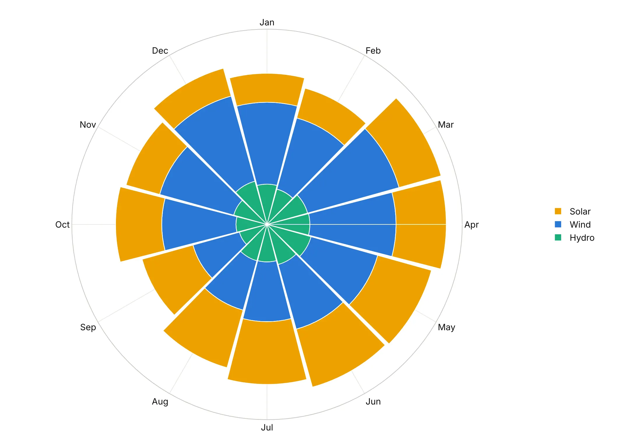
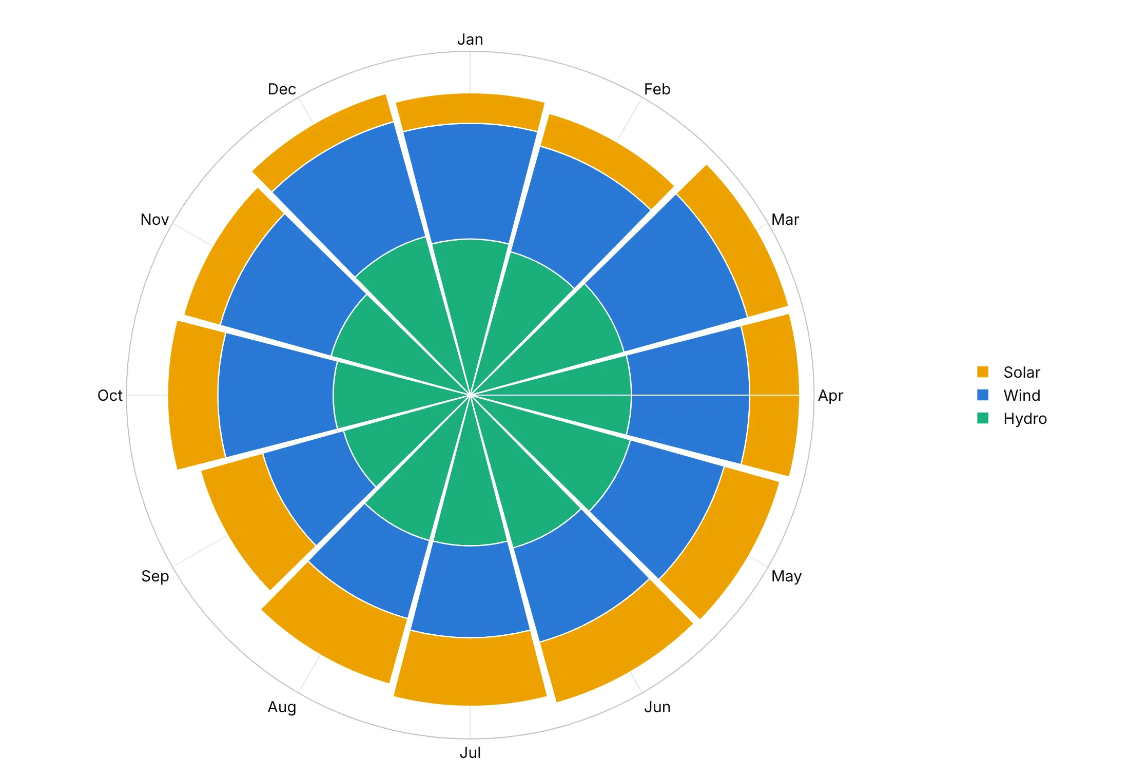
A wedge's area grows with the square of its radius, so when the radius is the value, the outer layers look bigger than they are. These are the 2025 wind, solar and hydro numbers both ways.

Radius proportional to the value. Plain stacked go.Barpolar bars make the outer solar layer look like the largest source, although solar generated 296 TWh in 2025 against 464 TWh from wind.

Area proportional to the value. Setting each layer's outer radius to the square root of the running total (base= for the inner edge) gives each source the area it earned, which is how Nightingale drew her diagram.

Checklist

Do

• Set rotation and direction for the reader's frame: rotation=90, direction="clockwise" for clocks, calendars and compasses.
• Use categories (or degrees you computed) for theta, and label hours, months and compass points by name.
• Start the radial axis at zero for bars, and say so when a line chart's axis starts elsewhere, as the climate spiral's does at -1 °C.
• Use square-root radii when the wedges' area should carry the value.
• Join the last point to the first (line_close=True, or repeat the first point) so loops close.
• Write a title that states the takeaway and put the source in the subtitle.

Don't

• Use a polar chart for data with no direction or cycle; a bar or line chart reads more precisely.
• Compare values at angles far apart on the circle when exact differences matter.
• Stack many series in a polar bar chart with linear radii; the outer one will look too big.
• Let radial tick labels sit on top of bars or lines.

Options to customize

These are the options that matter most for go.Scatterpolar, go.Barpolar and the layout.polar axes they share. The full lists are in the scatterpolar reference, the barpolar reference and the layout.polar reference.

1. r, theta: the distance from the center and the angle, in degrees for numbers and evenly spaced for categories.
2. thetaunit: "radians" if your angles are in radians.
3. mode (scatterpolar): markers for a polar scatter chart, lines for a polar line chart, or both.
4. px.line_polar(line_close=True): closes each loop by joining the last point to the first.
5. go.Scatterpolargl or render_mode="webgl": WebGL markers for tens of thousands to a million points.
6. base (barpolar): where each bar starts, for stacked area-true wedges and for bars that start at a reference ring.
7. polar.barmode: stack for stacked bars, overlay for wedges measured from the center, as in Nightingale's diagram.
8. polar.bargap: the gap between wedges; 0 for touching bins.
9. polar.angularaxis.rotation, direction: where 0 or the first category sits and which way angles run; 90 and clockwise for a clock or a compass.
10. polar.angularaxis.categoryarray, tickvals, ticktext: the order of categories and which labels to show.
11. polar.radialaxis.range: a fixed scale, which can start below zero for anomalies or returns.
12. polar.radialaxis.angle, tickangle: where the radial tick labels sit, so they don't cover the data.
13. polar.hole: an empty center, as a fraction of the radius.
14. polar.sector: draw only part of the circle, such as [0, 180] for a half circle.
15. polar.domain: place several polar charts side by side, as in the quarry blasts example.

More polar chart examples

Six more polar charts built from real public data, each with its source, the technique that makes it work and a prompt to rebuild it.

1. Arctic sea ice by day of the year, a polar line chart

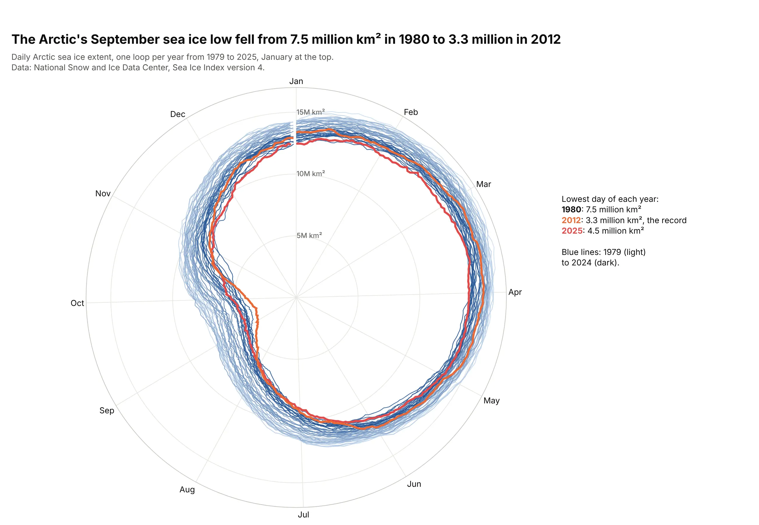
The lowest daily Arctic sea ice extent fell from 7.5 million km² in September 1980 to 3.3 million in September 2012, the record. On a circle, every year is one loop and the September dent moves toward the center. Data: National Snow and Ice Data Center, Sea Ice Index version 4.

Tip: draw dozens of years as thin lines in one light-to-dark color, and only the years in the story in strong colors on top.

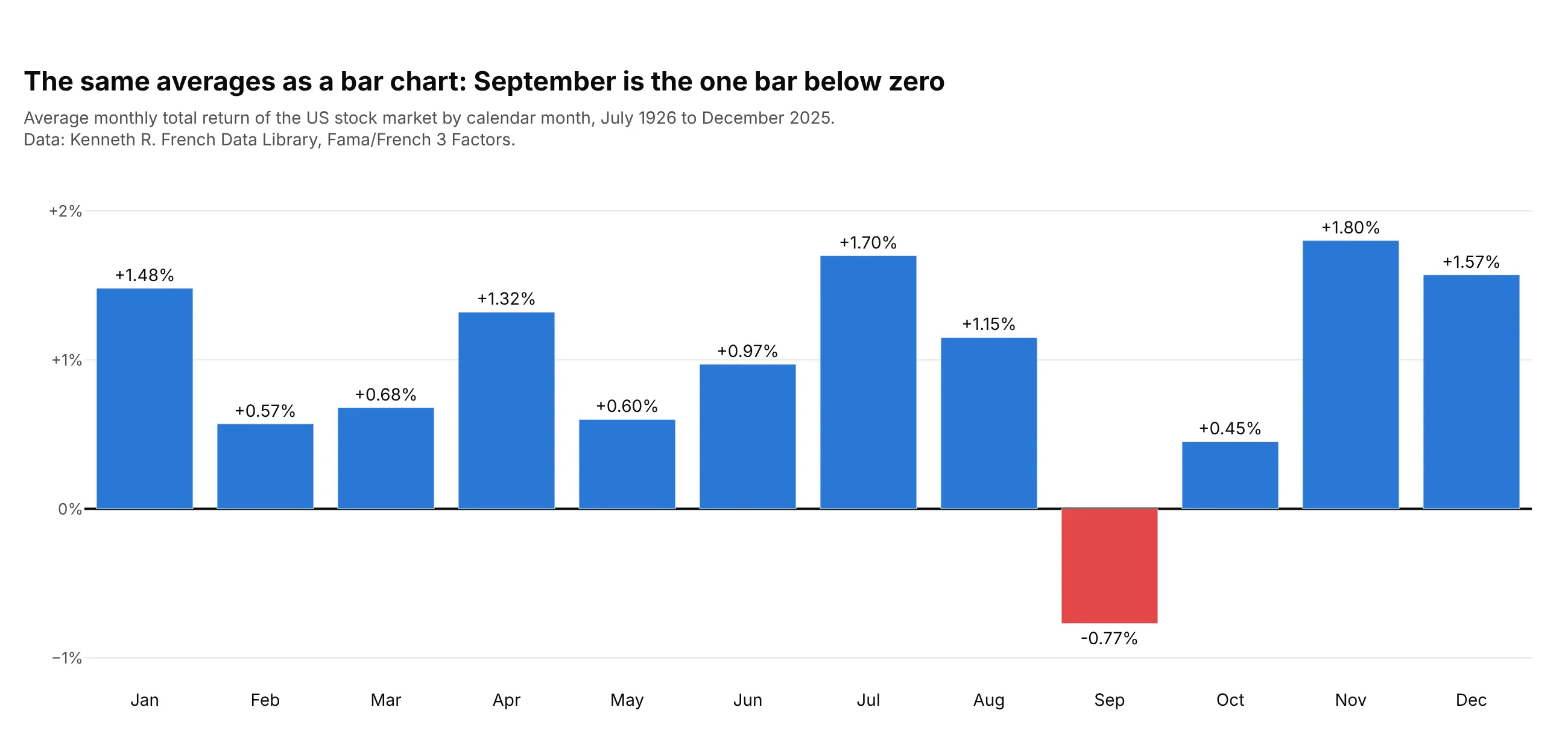
2. Stock market returns by calendar month, a polar bar chart example with negative values

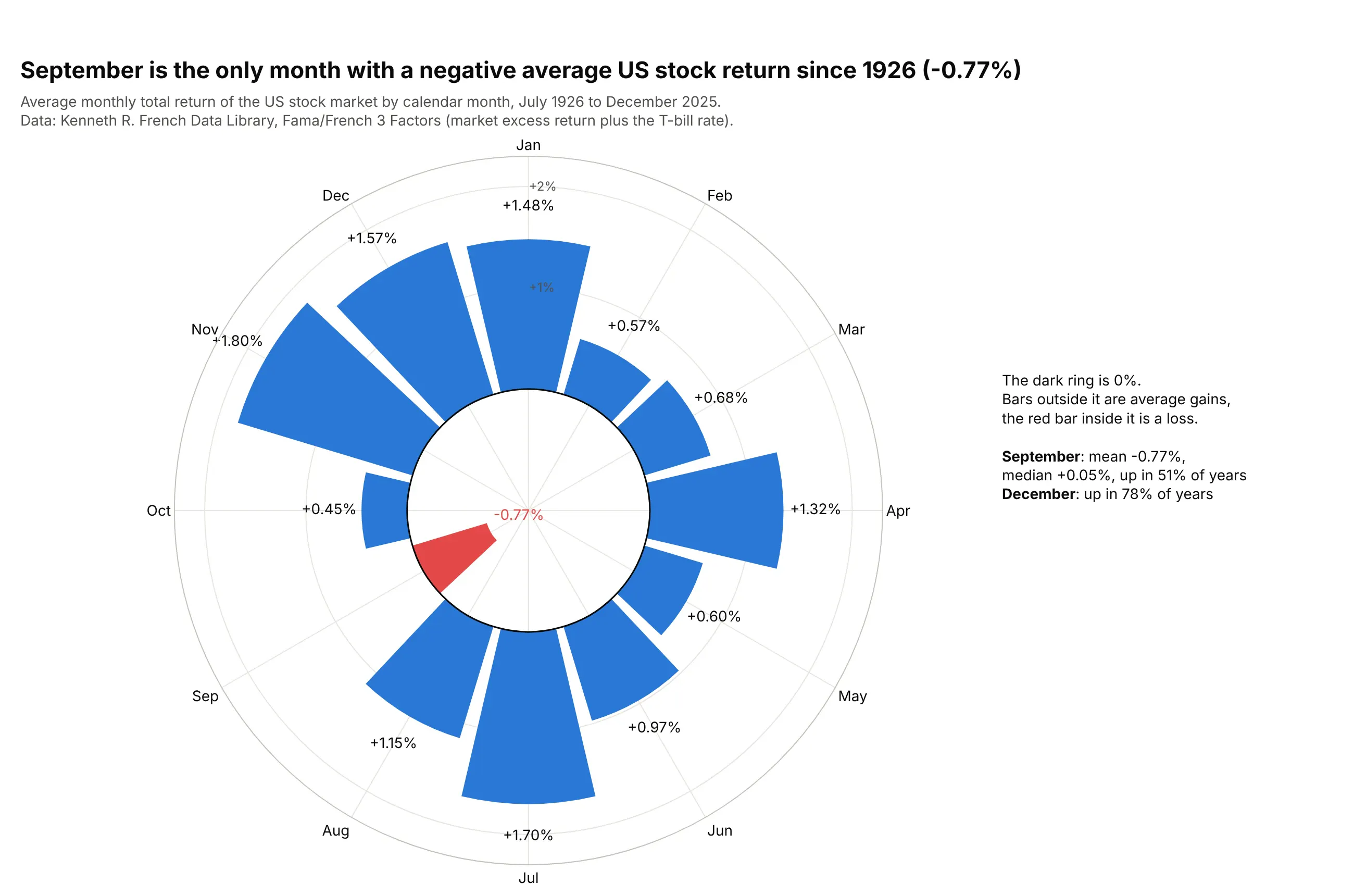
September is the only calendar month with a negative average US stock return from July 1926 to December 2025, at -0.77%, and it rose in only 51 of 100 years. The radial axis starts at -1.2%, so 0% is a ring and the losing month points inward. Data: Kenneth R. French Data Library, Fama/French 3 Factors.

Tip: with negative values, set radialaxis.range below zero and draw the zero ring as its own dark line, so readers can see where a bar changes direction.

Another way to see it: a plain bar chart puts the twelve averages on one straight baseline, which reads the size of each month more precisely than wedges on a circle.

3. Every hour of wind at a buoy off Long Island, a polar scatter chart

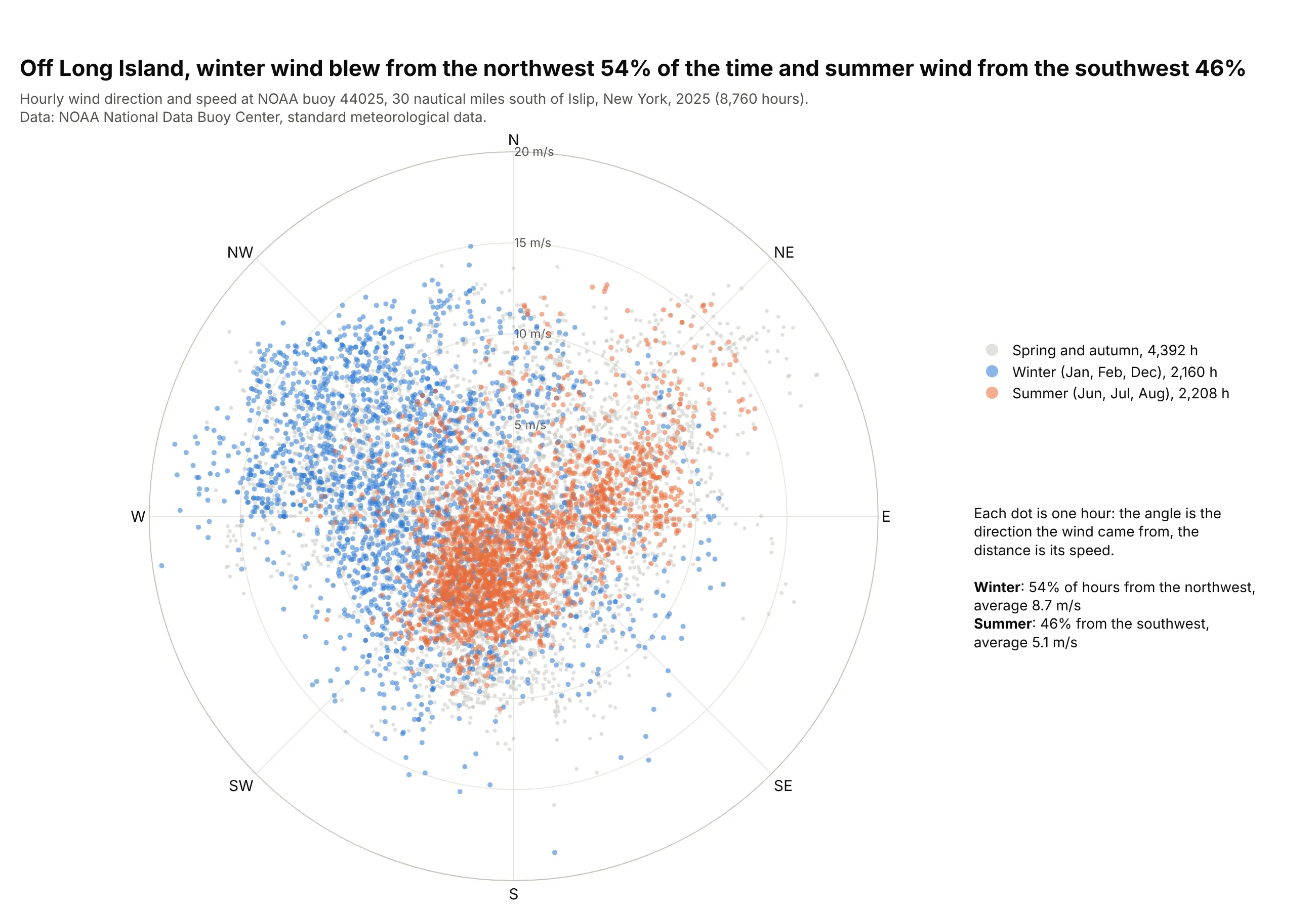
In 2025, the wind 30 nautical miles south of Islip, New York, came from the northwest in 54% of winter hours and from the southwest in 46% of summer hours, and averaged 8.7 m/s in winter against 5.1 m/s in summer. Each dot is one hour, so nothing is binned. Data: NOAA National Data Buoy Center, station 44025.

Tip: go.Scatterpolargl draws all 8,760 hours quickly, and coloring two seasons over the rest in light gray shows the shift without binning; the wind rose guide bins the same kind of data.

4. US births by day of the year

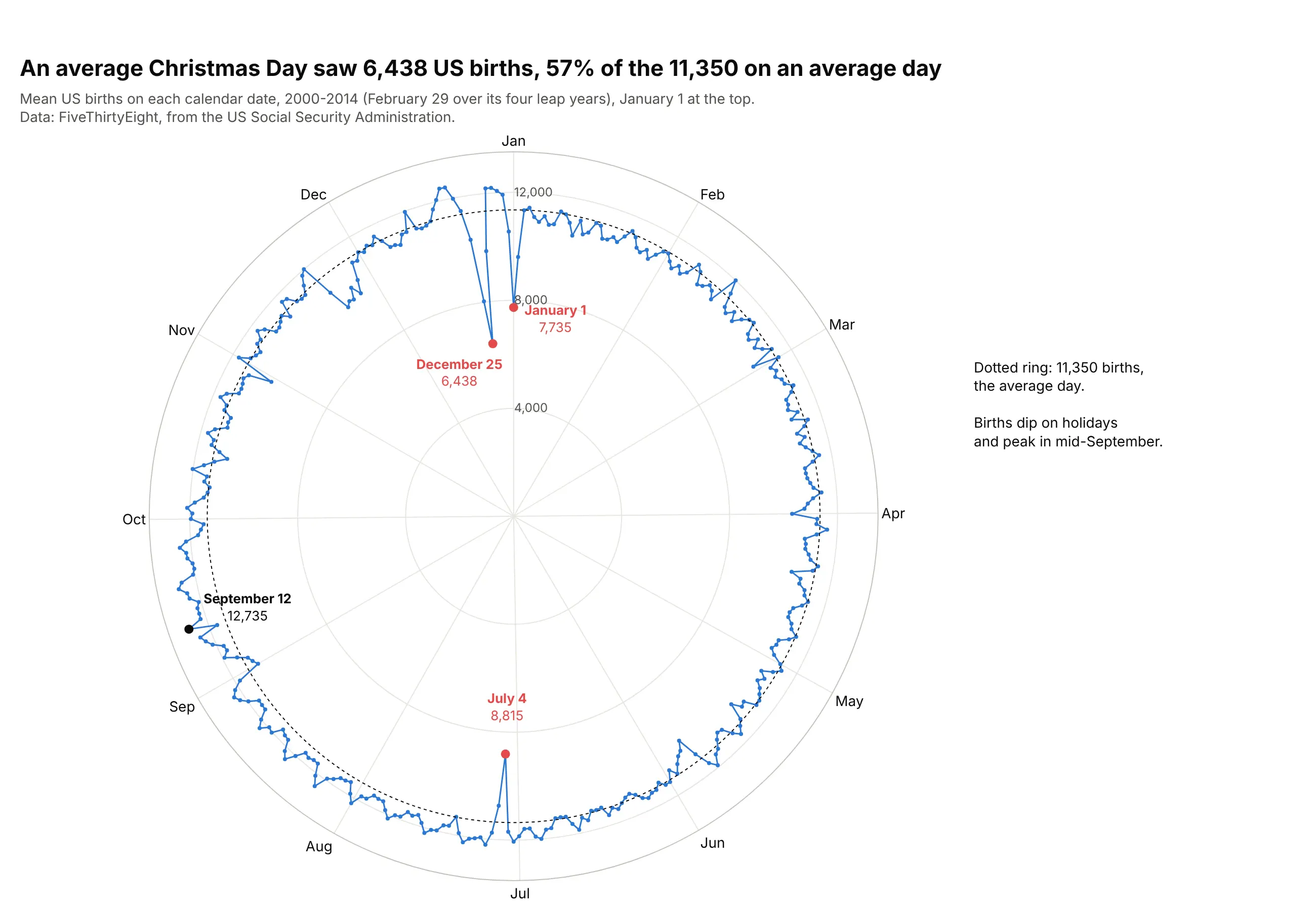
From 2000 to 2014, an average Christmas Day had 6,438 US births, 57% of the 11,350 on an average day, and January 1 and July 4 also dip. On a circle, the Christmas and New Year dips sit next to each other instead of at opposite ends of an axis. Data: FiveThirtyEight, from the US Social Security Administration.

Tip: start the radial axis at zero for counts, so a dip to 57% looks like 57%, and add a dotted ring at the average.

5. The orbits of the inner planets as polar curves

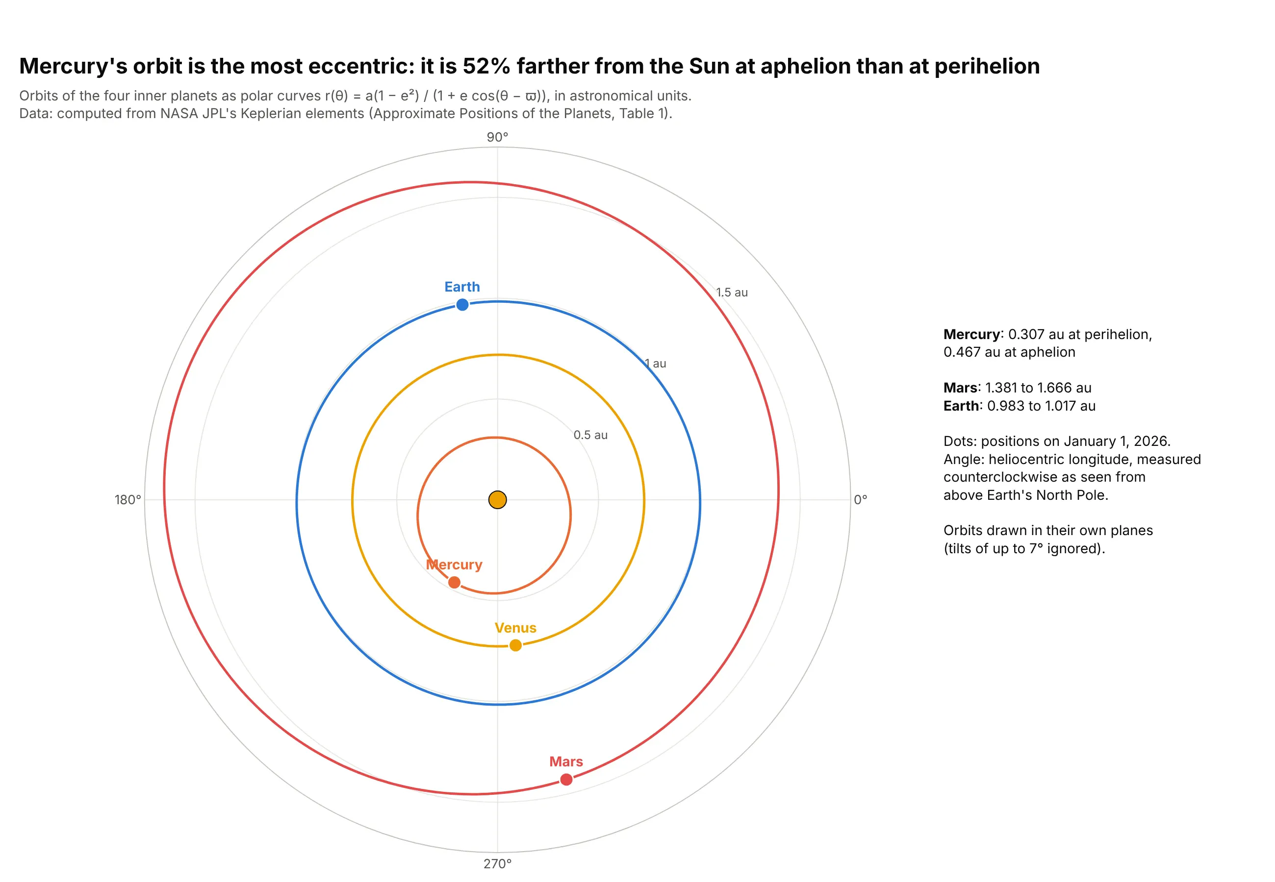
Mercury is 52% farther from the Sun at aphelion (0.467 au) than at perihelion (0.307 au), the most eccentric orbit of the four inner planets, while Earth only varies from 0.983 to 1.017 au. An orbit is a polar equation r(θ), the textbook use of polar coordinates. Data: computed from NASA JPL's Keplerian elements.

Tip: for astronomy and mathematics keep Plotly's default orientation (0° on the right, counterclockwise), because that's the convention readers expect.

6. Texas's power grid on a 24-hour clock

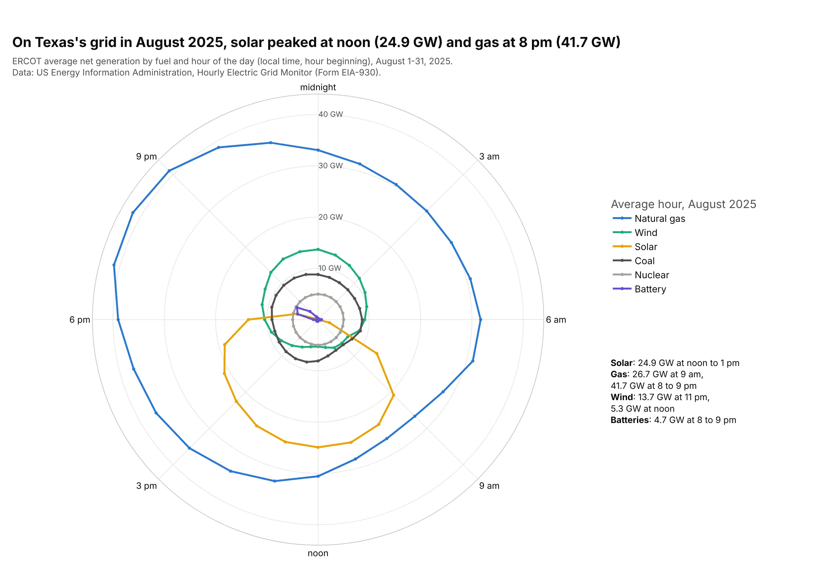
On ERCOT's grid in August 2025, solar averaged 24.9 GW at noon, a third of generation in that hour, and gas peaked at 41.7 GW between 8 and 9 pm as the sun set. Wind ran highest at 11 pm and batteries discharged most at 8 pm. Data: US Energy Information Administration, Hourly Electric Grid Monitor (Form EIA-930).

Tip: close each loop by repeating the first hour at the end, so the line from 11 pm back to midnight isn't missing.