Chris Parmer

October 24, 2026

Radar Charts - A Complete Guide

TL;DR

A radar chart draws several measures as spokes from a center and joins one item's values into a polygon, so each item becomes a shape you can recognize.
Radar charts are also known as spider charts, web charts, star plots and Kiviat diagrams, and are similar to parallel coordinates plots and wind roses.
Use one for a few profiles on axes that share a scale (percentiles, a share of a benchmark), for one profile against a benchmark ring, and for cycles such as months, hours or wind direction.
Use a dot plot or bars when exact values matter, small multiples or parallel coordinates for more than two or three items, and never compare polygon areas, because they change with the order of the axes.
Any coding agent can make one with Plotly in a minute. In Python it's px.line_polar(df, r=..., theta=..., line_close=True).

What is a radar chart?

Radar charts look like this:

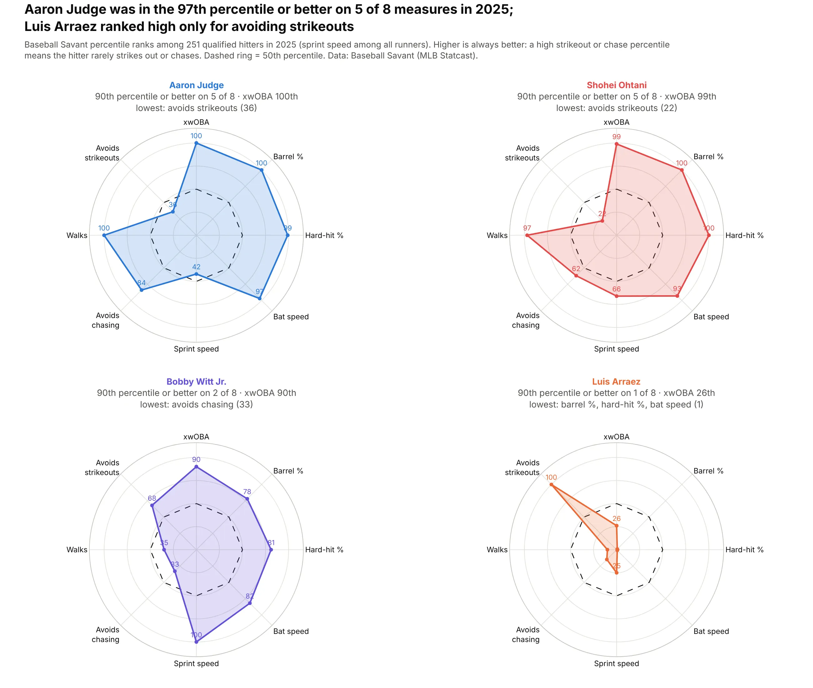
Four radar charts of 2025 Statcast percentile ranks with a dashed 50th percentile ring. Aaron Judge is at 97 or better on five of eight measures; Luis Arraez is at the 100th percentile for avoiding strikeouts and the 1st for barrels, hard hits and bat speed

Data: Baseball Savant (MLB Statcast), 2025.

How do you read a radar chart? In the example above, notice these things:

Each of the four charts is one hitter, and each of the eight spokes is one Statcast measure. The dot on a spoke is the hitter's percentile rank on that measure among qualified hitters (among all runners for sprint speed), so a dot at the edge means he was at the top of the league.
Strikeouts and chasing are ranked so that a high percentile means the hitter rarely does them, so outward always means better and a shape that reaches the edge on many spokes belongs to a strong all-round hitter. Aaron Judge is near the edge, at the 97th percentile or better, on five of the eight spokes.
The dashed ring is the 50th percentile, which shows at a glance where a hitter is above or below average. Luis Arraez is inside the ring on every spoke except avoiding strikeouts, which makes his shape a single spike.
Power measures sit on the right and plate discipline on the left, so the direction a shape leans tells you what kind of hitter it is. Bobby Witt Jr.'s shape stretches down toward sprint speed, where he ranks in the 100th percentile.
The area of a shape depends on the order of the spokes, and the same eight percentiles in a different order would draw a different shape. When you compare hitters closely, read the dots on each spoke.

It's often used for charts like these:

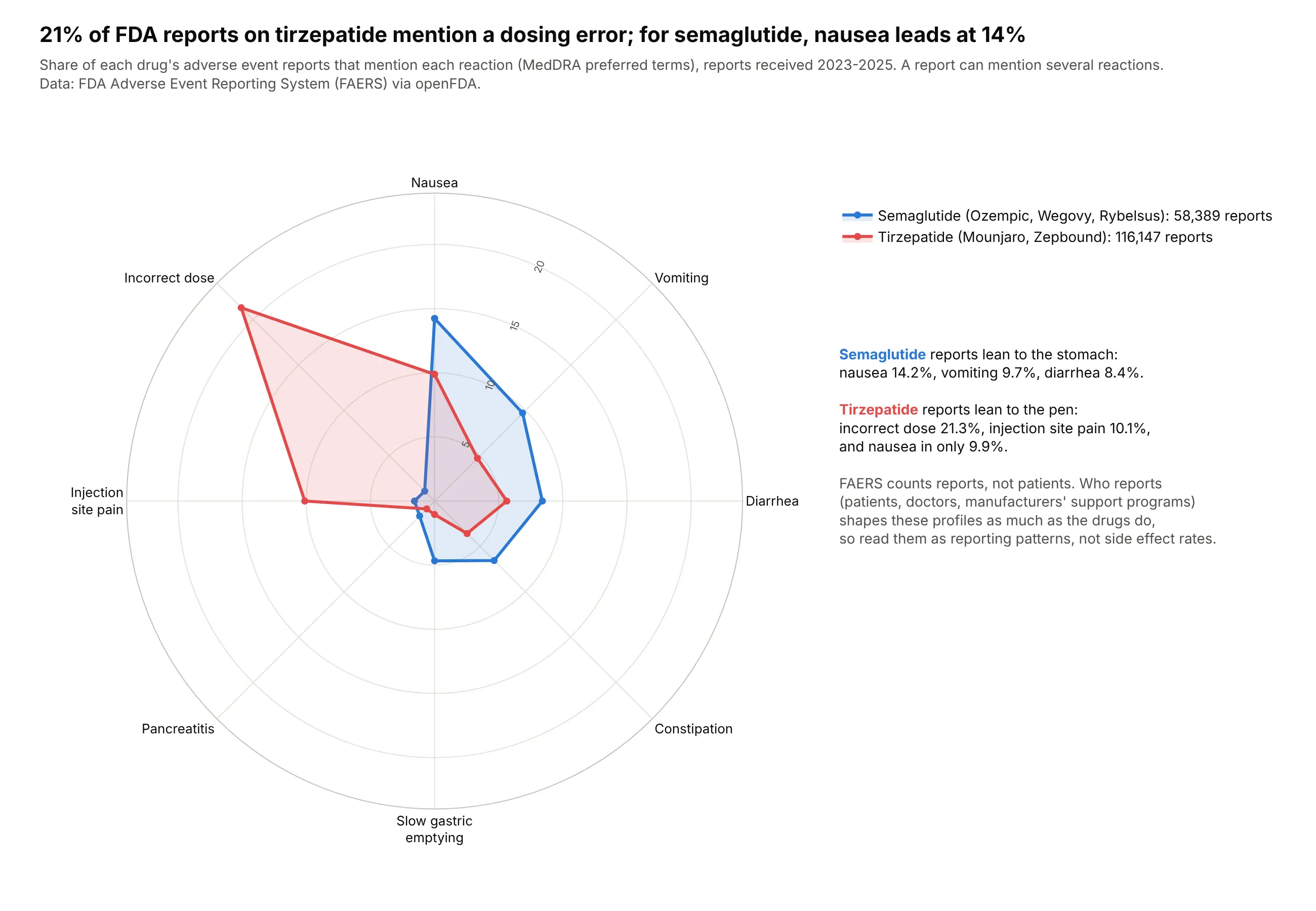
Radar chart of the share of FDA adverse event reports from 2023 to 2025 mentioning eight reactions, for semaglutide and tirzepatide. Semaglutide's shape leans to nausea (14.2%), tirzepatide's to incorrect dose (21.3%) and injection site pain (10.1%)

Two profiles against each other. 21% of FDA adverse event reports on tirzepatide mention a dosing error, while semaglutide's reports lead with nausea at 14% (these are reporting patterns, not side effect rates). Data: FDA FAERS via openFDA, 2023-2025.

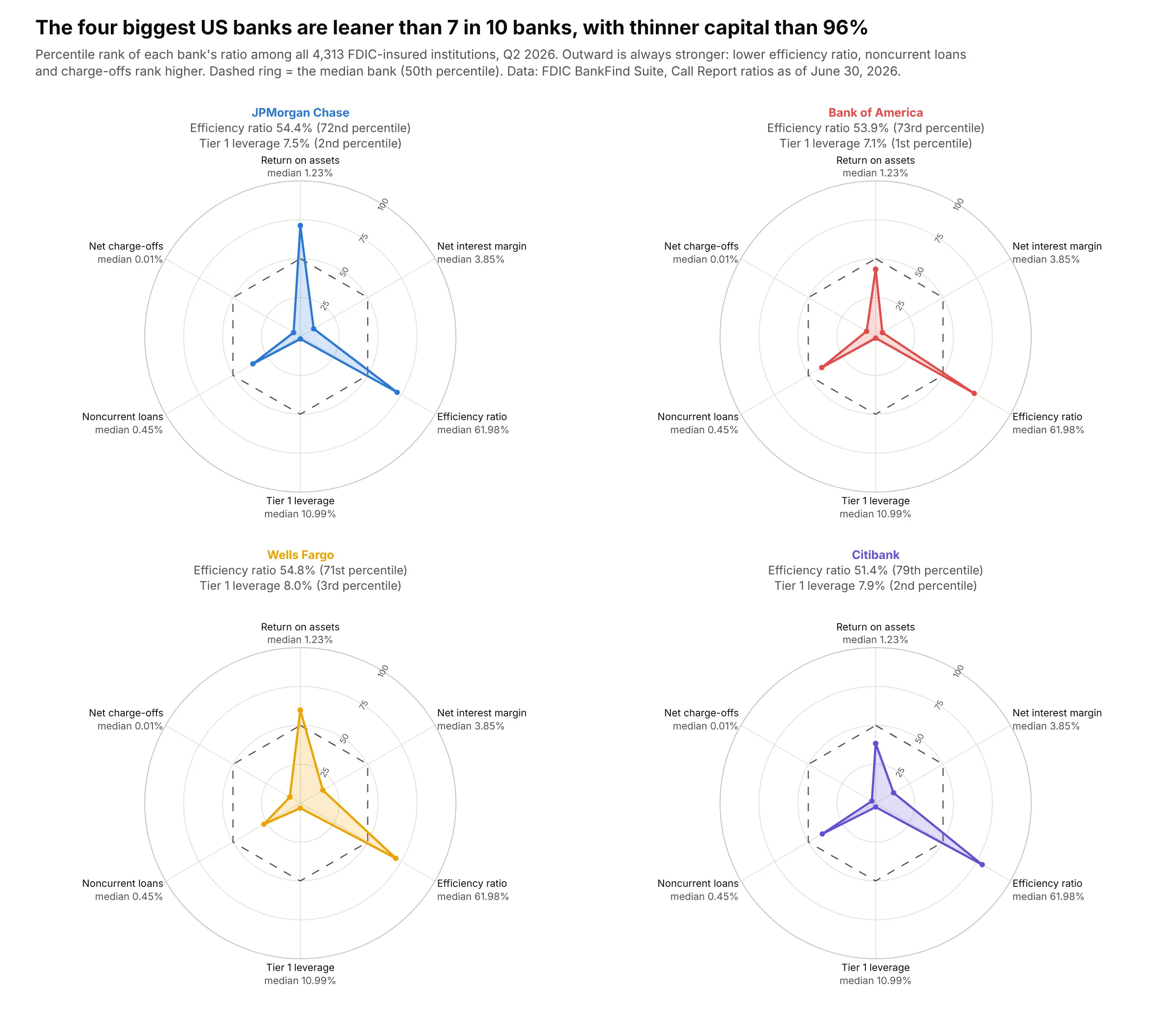
Four radar charts of percentile ranks among 4,313 FDIC-insured institutions in Q2 2026. JPMorgan, Bank of America, Wells Fargo and Citibank rank in the 71st to 79th percentile on efficiency and the 1st to 3rd on Tier 1 leverage, with a dashed ring at the 50th percentile

One profile against a benchmark. Ranked against all 4,313 insured banks, the four biggest US banks are more efficient than about 7 in 10 but sit in the bottom 4% on Tier 1 capital to average assets (7.1% to 8.0%, against a median of 11.0%). Data: FDIC BankFind Suite, Call Reports, June 30, 2026.

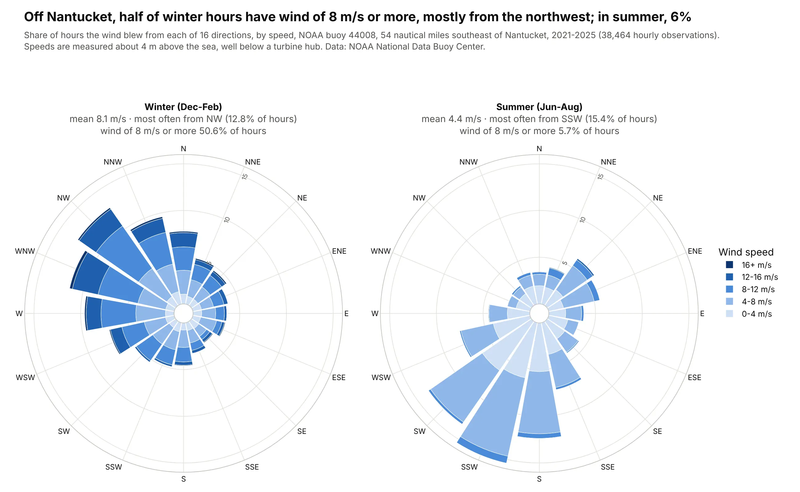
Two wind roses for NOAA buoy 44008 off Nantucket, 2021-2025. In winter the wind blows most often from the northwest and is 8 m/s or more 50.6% of the time; in summer it comes from the south-southwest and reaches 8 m/s only 5.7% of the time

A wind rose, the polar bar chart of directions. Off Nantucket, near the New England offshore wind leases, the wind blows at 8 m/s or more in 50.6% of winter hours, mostly from the northwest, and in 5.7% of summer hours. Data: NOAA National Data Buoy Center, buoy 44008, 2021-2025.

A short history

The star chart is commonly credited to the German statistician Georg von Mayr, who used it in an 1877 book of social statistics. Its polar bar cousin is older: in 1858 Florence Nightingale drew the deaths in the British army in the Crimean War as a rose of monthly wedges, to show that most soldiers died of preventable disease rather than wounds. Here is her diagram, redrawn with Plotly from her own numbers:

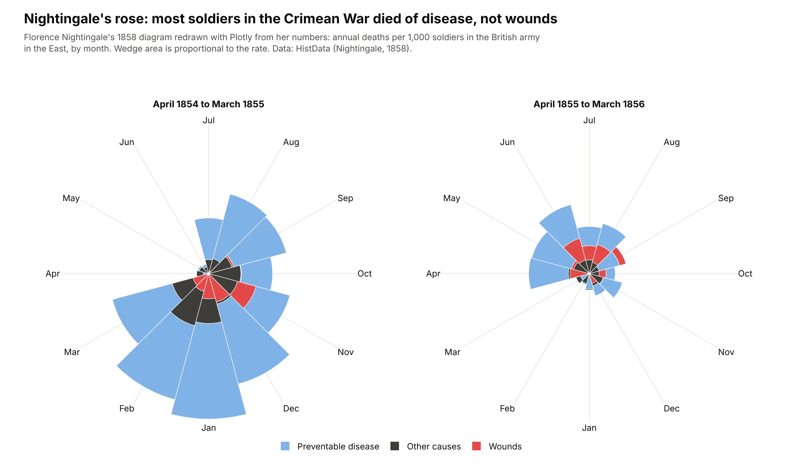
Florence Nightingale's 1858 rose diagram redrawn with Plotly: two polar area charts of annual deaths per 1,000 soldiers in the British army in the East, April 1854 to March 1855 and April 1855 to March 1856, with large blue wedges for preventable disease peaking in January 1855, much smaller red wedges for wounds and dark wedges for other causes

In the first year, 11,157 of the 13,294 deaths (84%) were from disease and 772 from wounds. In computing, Kenneth Kolence and Philip Kiviat used the star form for system performance profiles in 1973, which is why it's still called a Kiviat diagram there, and sports and video games later made the player "spider chart" familiar to everyone else.

Alternatives to a radar chart

Here's the same set of sector ETF profiles drawn six ways. Some are better for the question, some worse, some just different:

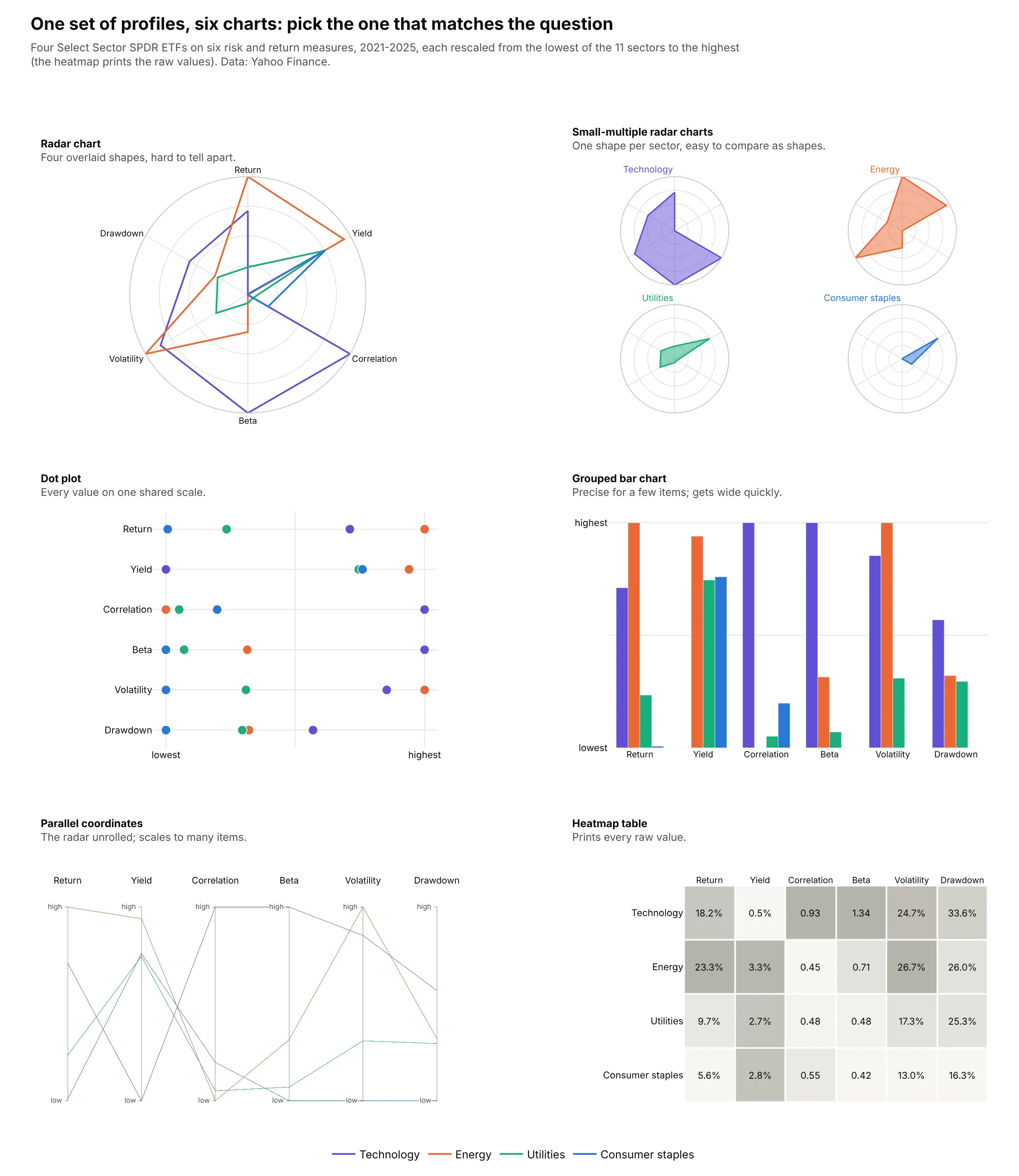
The same four sector ETFs (technology, energy, utilities and consumer staples) on six risk and return measures, 2021-2025, drawn six ways: one radar chart with four overlaid shapes, four small-multiple radar charts, a dot plot, a grouped bar chart, parallel coordinates and a heatmap table of the raw values, from energy's 23.3% annual return to technology's beta of 1.34

Dot plot (better for precise comparisons). It puts every value on one straight, shared scale, and people judge positions on a common scale more accurately than angles or areas (Cleveland and McGill, 1984; Heer and Bostock, 2010). Radial layouts were slower than Cartesian ones for most tasks in Diehl, Beck and Burch's study.
Small-multiple radar charts (better for more than two items). One shape per panel keeps the thing radar charts are good at, recognizing a profile, without the tangle of overlaid shapes.
Grouped bar chart (works too, for a few items). It's as precise as the dot plot, but it gets wide as items and measures multiply.
Parallel coordinates (better for many items). These are the radar chart's polylines unrolled onto parallel vertical axes, and they scale to dozens of items and axes. See our parallel coordinates plot guide.
Heatmap table (better when every value matters). It prints the raw value in every cell and can be sorted by any column, at the cost of any sense of shape. See our heatmap guide.
Overlaid radar chart (worse for three or more items). In a test of charts for composite indicators, Albo et al. found the radar chart the least effective and least liked of three radial designs.

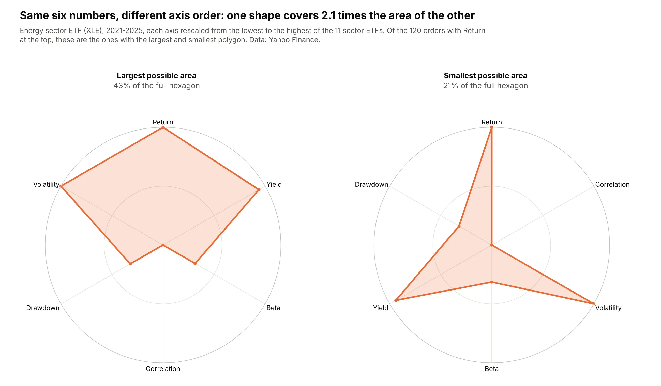
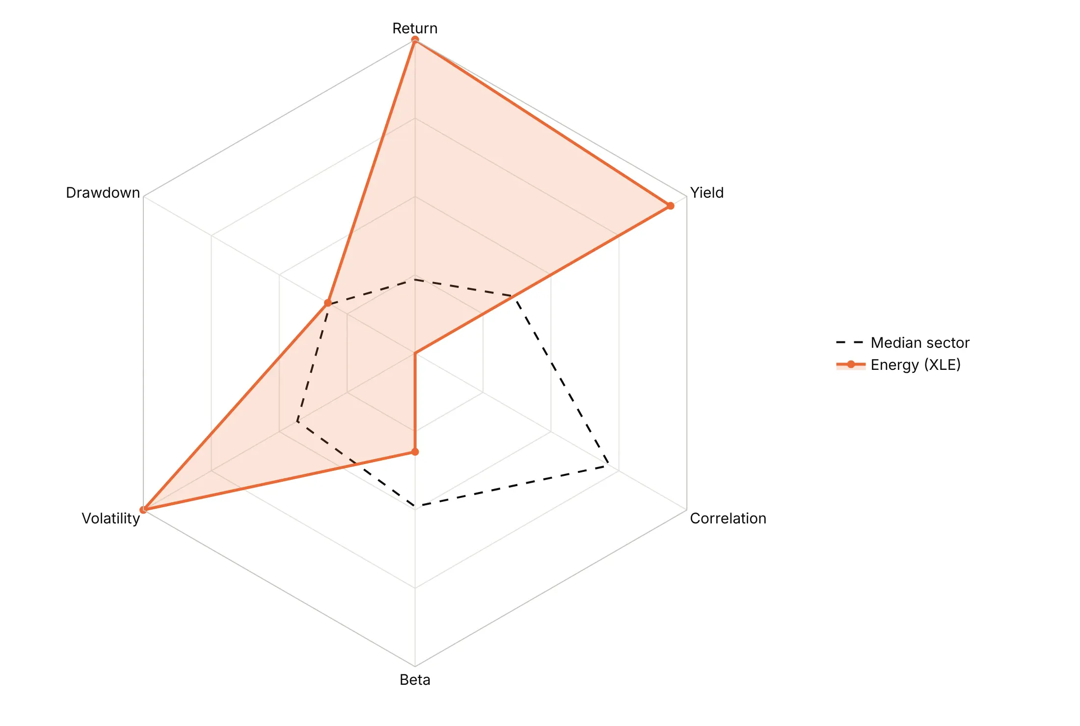
Here's where any of the straight-axis charts wins. The polygon's area depends on the order of the axes, not just on the data, so the same six numbers for the energy sector ETF cover 43% of the full hexagon in one order and 21% in another:

The energy sector ETF's six rescaled risk and return measures in two axis orders, the largest possible polygon covering 43% of the hexagon and the smallest 21%, 2.1 times the area for the same numbers

How to make a radar chart

With AI

ChatGPT, Claude Code, GitHub Copilot, Cursor and other AI tools are excellent at writing Plotly code. Name Plotly in the prompt, say how to scale the axes and which way is better, and list the checks you want:

Make a plotly radar chart from profiles.csv (columns: item, metric, value).

- Pivot to one row per item. Rescale each metric from its minimum (0) to its maximum (1)
  across items, and flip metrics where lower is better so outward always means better.
  Say how the axes were rescaled in the subtitle.
- One small multiple per item (make_subplots with type "polar"), go.Scatterpolar with
  fill="toself", the polygon closed by repeating the first point, and a dashed median ring.
- Related metrics next to each other; angularaxis rotation=90, direction="clockwise".
- A title that states the main takeaway.
- Check that every metric has a value for every item, and print the min and max per metric.
- Save it as radar.html and as a PNG at 2x scale.

With Plotly Studio

Plotly Studio is a desktop app where you point an AI at a dataset and it builds charts and a Dash app around your questions. Ask for a radar chart the same way:

Show a radar chart of each bank's financial ratios as percentile ranks among all banks, flipped so outward is always stronger, with a dashed ring at the 50th percentile. One small multiple per bank, and a dropdown to pick which banks to show.

Make a radar chart in Python or JavaScript

This is the code AI tools write under the hood. In Python, Plotly Express draws a radar chart from a long table with one row per item and measure:

import pandas as pd
import plotly.express as px

df = pd.DataFrame({
    "player": ["Judge"] * 5 + ["Arraez"] * 5,
    "stat": ["xwOBA", "Barrel %", "Walk %", "Avoids strikeouts", "Sprint speed"] * 2,
    "percentile": [100, 100, 100, 36, 42, 26, 1, 10, 100, 25],
})
fig = px.line_polar(df, r="percentile", theta="stat", color="player", line_close=True, range_r=[0, 100])
fig.update_traces(fill="toself")
fig.show()

In JavaScript, plotly.js takes one scatterpolar trace per item. Repeat the first point at the end to close the polygon:

<div id="chart"></div>
<script src="https://cdn.plot.ly/plotly-4.1.1.min.js"></script>
<script>
  const stats = ["xwOBA", "Barrel %", "Walk %", "Avoids strikeouts", "Sprint speed", "xwOBA"];
  Plotly.newPlot("chart", [
    {type: "scatterpolar", name: "Judge", r: [100, 100, 100, 36, 42, 100], theta: stats, fill: "toself"},
    {type: "scatterpolar", name: "Arraez", r: [26, 1, 10, 100, 25, 26], theta: stats, fill: "toself"}
  ], {polar: {radialaxis: {range: [0, 100]}, angularaxis: {rotation: 90, direction: "clockwise"}}});
</script>

For a wind rose, use go.Barpolar (type: "barpolar" in JavaScript) with one trace per speed band and polar.barmode="stack".

Share it

Every Plotly chart has a Share chart button (the cloud icon in its toolbar) that uploads it to Plotly Cloud and gives you a link. Only you can see it until you change its visibility.

For a live app, put the chart in a Dash app and publish it with the Plotly Cloud CLI. Coding agents can run these commands for you:

pip install "dash[cloud]"
plotly user login
plotly app publish

If your data has to stay in your own cloud or data center, publish to Dash Enterprise instead.

Dos and don'ts

Plotly's defaults draw raw values on one radial axis, with a color and a filled shape for each series. For a chart you publish, most of the work is rescaling the axes and deciding what to leave out. Here is the same sector ETF data both ways.

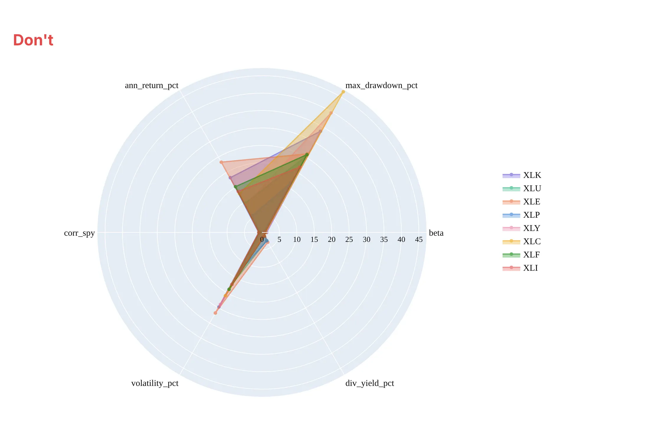
Don't plot raw values in different units on one radial axis, where a drawdown of up to 47% flattens betas and correlations under 1.4, label the axes with column names, or overlay eight filled shapes:

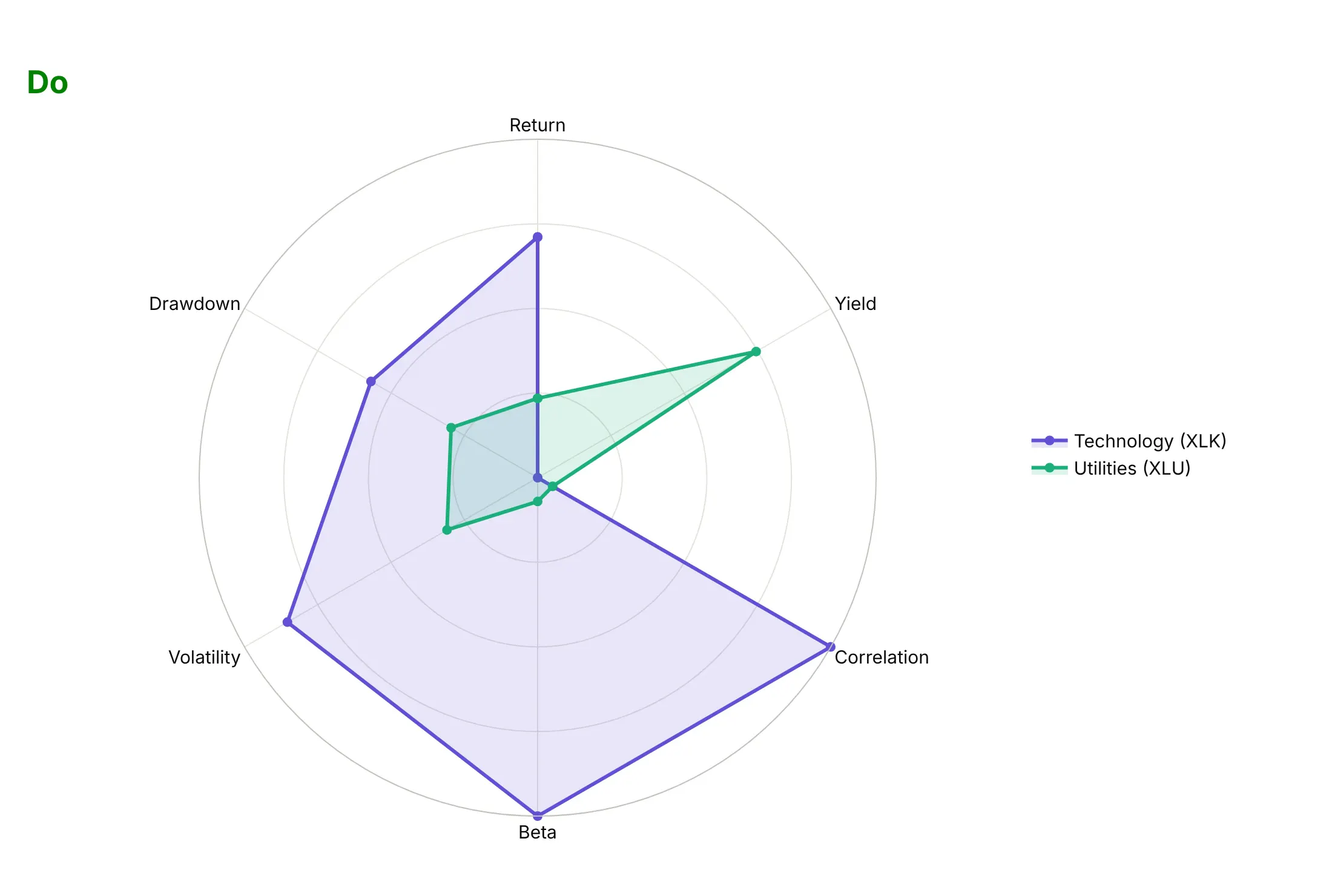
A radar chart of eight sector ETFs with plotly-style defaults: raw values in five different units on one radial axis from 0 to 45, column names such as max_drawdown_pct as axis labels, eight overlapping filled shapes in the same palette as the next chart and a serif font

Do rescale each axis (here from the lowest of the 11 sector ETFs to the highest), compare two series, and keep return and yield next to each other and the risk measures together:

The same data designed on purpose: technology in purple and utilities in green on six rescaled axes named Return, Yield, Correlation, Beta, Volatility and Drawdown, with technology reaching the edge on beta and correlation and utilities spiking toward yield

With many series, show one at a time

Here are four ways to draw all 11 sector ETFs on the same six rescaled axes.

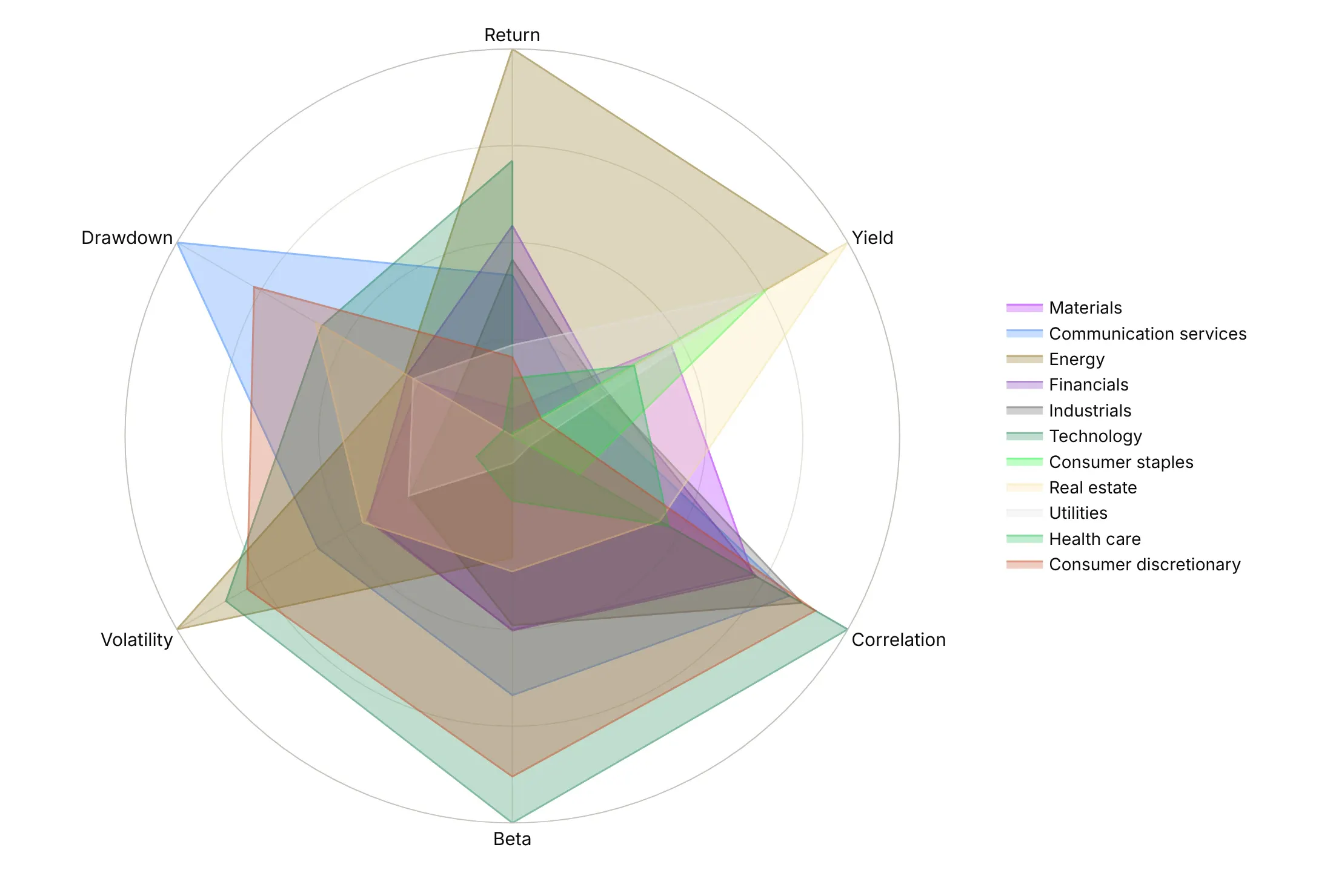
Every series in its own color (avoid). Eleven overlapping shapes, and the eye can't follow any of them.

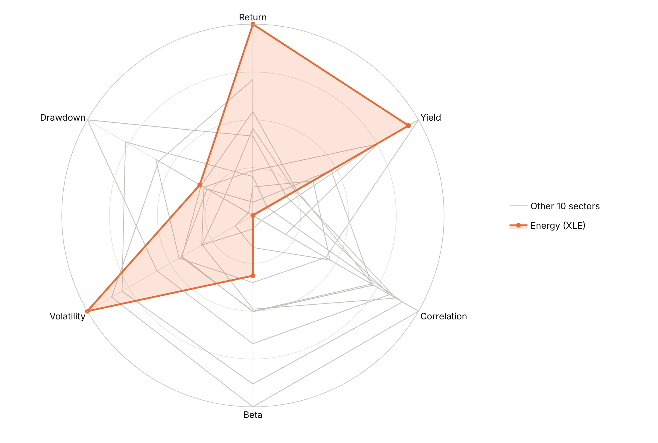
Eleven sector ETFs on one radar chart, each a filled shape in its own color, overlapping into a tangle in which no single sector can be followed

Highlight one, gray the rest. Energy stands out, and the gray outlines still show the range of the other ten sectors.

The 11 sector ETFs with energy as a filled orange shape at or near the edge on return, yield and volatility, and the other ten sectors as thin gray outlines

One against a benchmark. Energy against the median of the 11 sectors, drawn as a dashed line, says where it's above or below a typical sector on each measure.

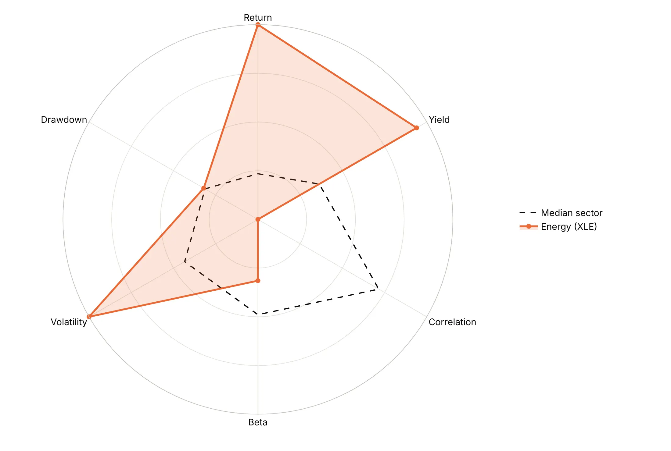
Energy as a filled orange shape against a dashed black line for the median of the 11 sector ETFs, with energy far outside the median on return, yield and volatility and inside it on correlation and beta

Polygon gridlines. polar.gridshape="linear" draws the rings as polygons, so they run parallel to the shape's edges.

The same energy against median comparison drawn on hexagonal gridlines instead of circles

Checklist

Write a title that states the takeaway.
Rescale every axis on purpose and say how: percentiles, min to max, a ratio to a benchmark or a fixed range per axis.
Point every axis the same way, so outward always means more, or always means better.
Start the radial axis at zero, or say on the chart where it starts.
Put related axes next to each other.
Draw a benchmark ring and label its value.
Label the values that matter on the points, and clip outliers at the edge with their real value as text.

Don't

Plot mixed units on one radial axis.
Overlay more than two or three filled shapes.
Rank items by polygon area.
Use a radar chart for a time series that isn't a cycle.
Rely on hover in a static image.

Options to customize

These are the go.Scatterpolar, go.Barpolar and polar layout options that matter most. The full list is in the Plotly radar chart documentation, the polar chart documentation and the scatterpolar reference.

px.line_polar(r, theta, color, line_close): a radar chart from a long DataFrame in one line; line_close=True closes the polygon.
go.Scatterpolar(r, theta): one polygon or line; repeat the first point at the end to close it.
fill="toself": fills the polygon. Keep fills light and use them for one or two shapes.
mode="lines+markers+text", text: points and value labels, to print the values that matter.
go.Barpolar(r, theta, width): one wedge per angle, for wind roses and calendar wheels.
polar.barmode: stack for speed bands in a wind rose, overlay for nested counts.
polar.radialaxis.range: the radial minimum and maximum. Start at 0, or say where it starts; use a negative minimum for values such as betas.
polar.radialaxis.tickvals, ticktext, angle: ring positions, their labels and the angle the labels sit at.
polar.angularaxis.rotation, direction: rotation=90, direction="clockwise" puts the first axis at 12 o'clock and runs clockwise.
polar.angularaxis.thetaunit, tickvals, ticktext: numeric angles with custom labels, for hours or calendar dates.
polar.gridshape: circular (default) or linear for polygon rings.
polar.hole: an empty center as a fraction of the radius, which keeps the lowest values off the exact center.
polar.domain: the position of a polar subplot, to put several radars or wind roses side by side.
make_subplots(specs=[[{"type": "polar"}] * n]): a grid of polar subplots for small multiples.
hovertemplate, customdata: hover text, to show the raw values behind rescaled axes.

More radar chart examples

Ten more radar and polar charts built from real public data, each with its source, the technique that makes it work and a prompt to rebuild it.

1. Factor ETFs against the S&P 500

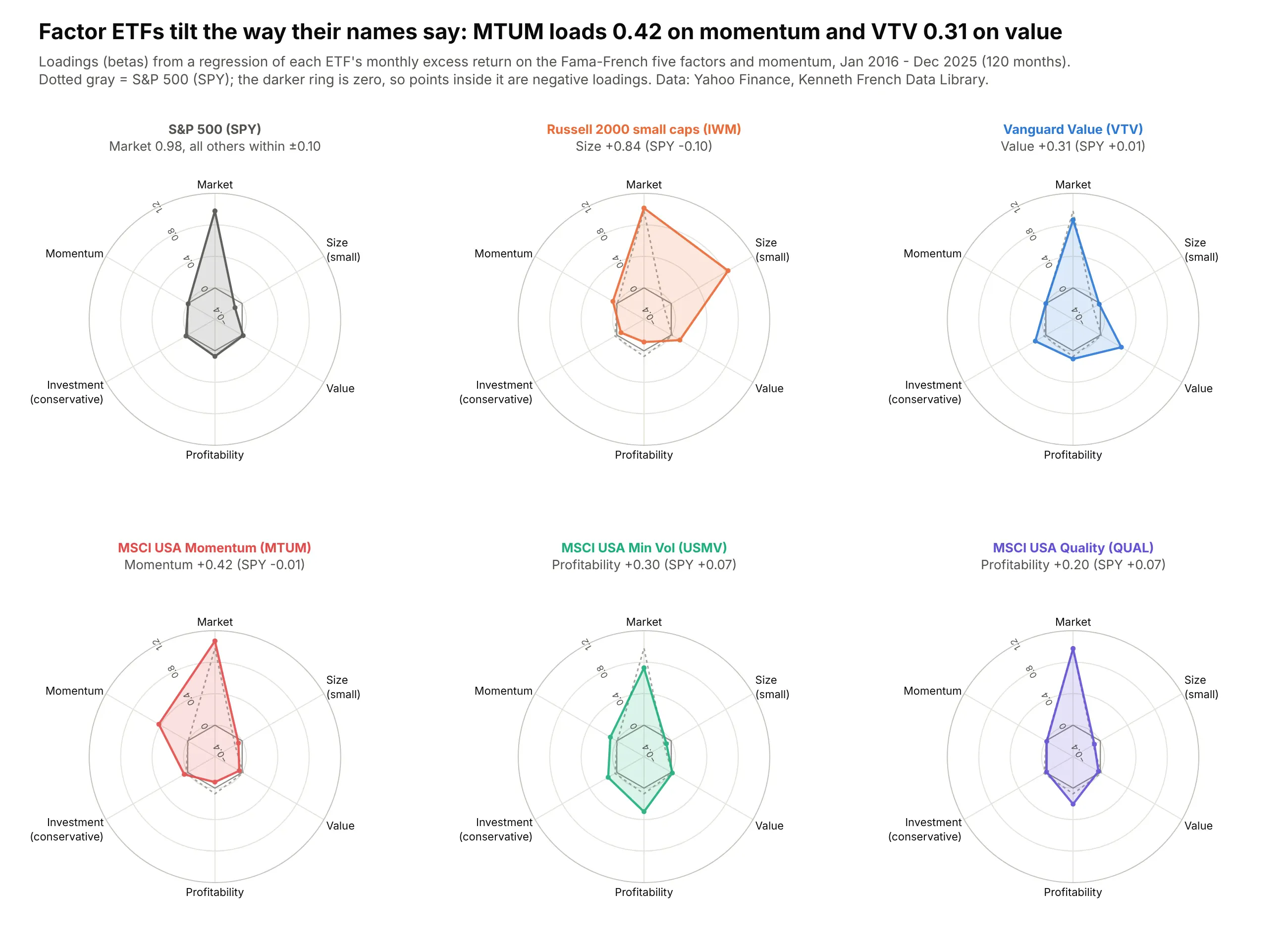
Six radar charts of factor loadings from 2016 to 2025: the S&P 500, then five factor ETFs each with the S&P 500 dotted behind. MTUM loads 0.42 on momentum, VTV 0.31 on value, IWM 0.84 on size, USMV 0.30 on profitability with a market beta of 0.73

Regressing ten years of monthly returns on the Fama-French factors shows each ETF tilting the way its name says. MTUM loads 0.42 on momentum and VTV 0.31 on value, where the S&P 500 is near zero on both. Data: Yahoo Finance; Kenneth French Data Library, 2016-2025.

Tip: betas can be negative, so the radial axis runs from -0.4 and a dark ring marks zero.

Get the data from Yahoo Finance (monthly dividend-adjusted closes for SPY, IWM, VTV, MTUM, USMV, QUAL)
and Kenneth French's Data Library (Fama-French 5 factors 2x3 and momentum, monthly, 2016-2025)
and regress each ETF's excess return on the six factors
(columns: etf, factor, beta).

Plot a 2x3 grid of plotly radar charts, one per ETF, with SPY as a dotted gray benchmark in each.
Radial axis from -0.4 to 1.2 with a dark ring at 0. Title the biggest tilt per panel.

2. Eleven sector ETFs, eleven risk profiles

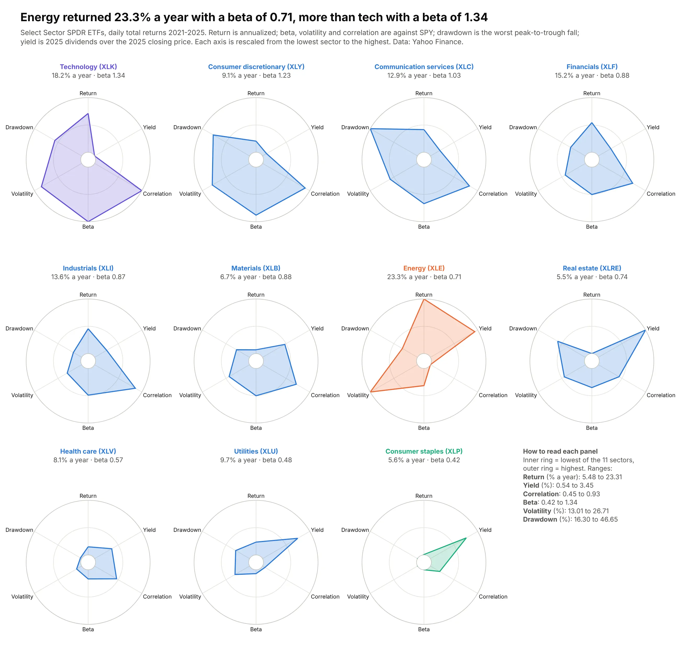
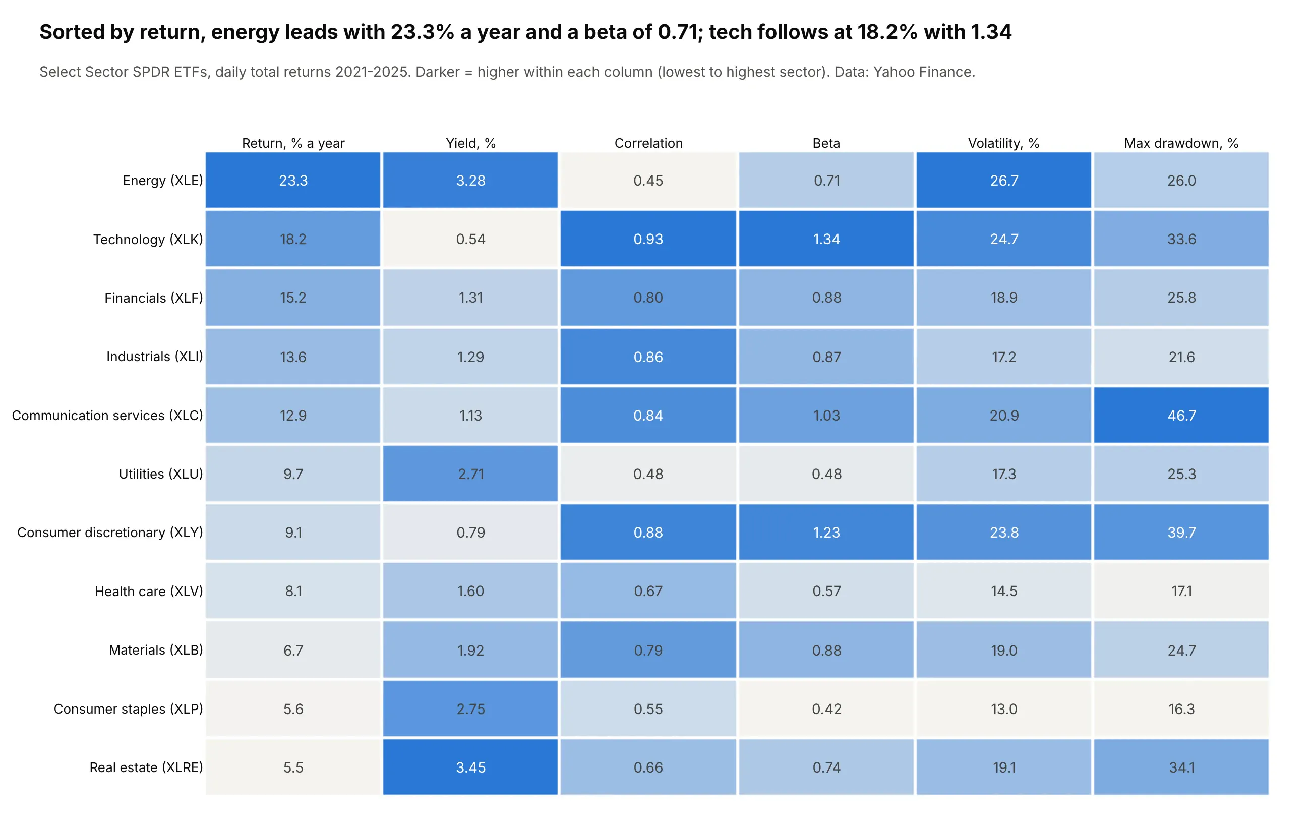
Eleven small radar charts of Select Sector SPDR ETFs on return, yield, correlation, beta, volatility and drawdown from 2021 to 2025, each axis rescaled from the lowest sector to the highest. Energy returned 23.3% a year with a beta of 0.71; tech 18.2% with a beta of 1.34

Small multiples sort sectors into families: compact defensive shapes (staples, utilities, health care), big high-beta ones (tech, discretionary) and energy on its own. Energy returned 23.3% a year from 2021 to 2025 with a beta of 0.71. Data: Yahoo Finance.

Tip: min-max rescaling per axis, with the ranges printed in the empty twelfth cell.

Get the data from Yahoo Finance (daily closes, adjusted closes and dividends, 2021-2025, for the
11 Select Sector SPDR ETFs and SPY) and compute per ETF
(columns: ticker, sector, ann_return_pct, volatility_pct, beta, max_drawdown_pct, div_yield_pct, corr_spy).

Rescale each metric min-max across the 11 ETFs and draw a 3x4 grid of plotly radar charts (polar.hole=0.12).
Return and yield on the right, risk measures on the left. Print each metric's range in the 12th cell.

Another way to see it: a heatmap table prints every raw value and sorts by any column.

A heatmap table of the 11 sector ETFs sorted by annual return, from energy at 23.3% to real estate at 5.5%, with yield, correlation, beta, volatility and drawdown printed in each cell

3. External risk in nine emerging markets

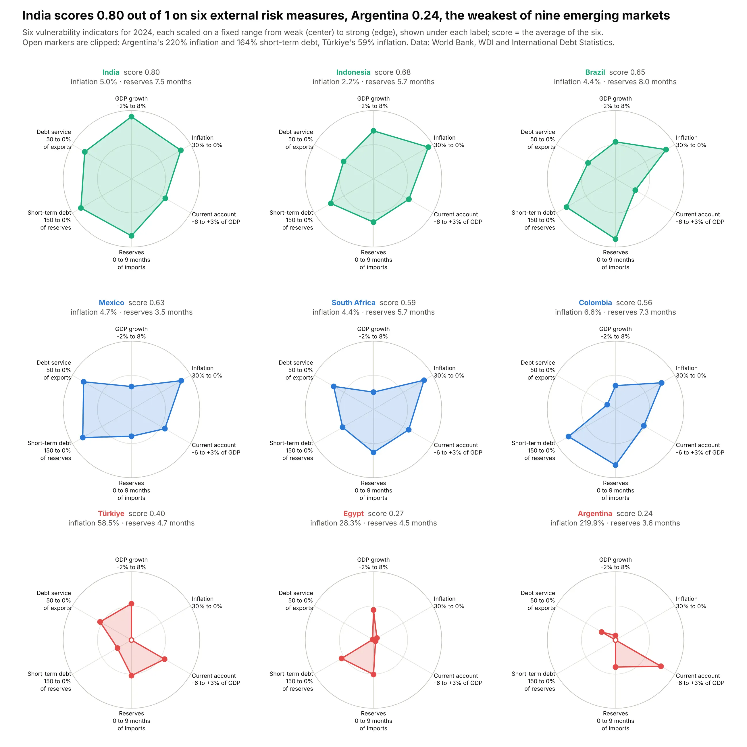
Nine radar charts of 2024 external vulnerability indicators on fixed scales, ordered by score: India 0.80, Indonesia 0.68, Brazil 0.65, Mexico 0.63, South Africa 0.59, Colombia 0.56, Türkiye 0.40, Egypt 0.27 and Argentina 0.24, with Argentina's 220% inflation clipped

On six World Bank indicators scaled to fixed thresholds, India scores 0.80 out of 1 and Argentina 0.24, and Argentina's 220% inflation runs off the scale. Data: World Bank WDI and International Debt Statistics, 2024.

Tip: a fixed range per axis (printed under each label) keeps magnitudes, and clipped values get an open marker.

Get the data from the World Bank API for 2024 (FP.CPI.TOTL.ZG, NY.GDP.MKTP.KD.ZG, BN.CAB.XOKA.GD.ZS,
FI.RES.TOTL.MO, DT.DOD.DSTC.IR.ZS, DT.TDS.DECT.EX.ZS) for ARG, TUR, EGY, ZAF, COL, BRA, MEX, IND, IDN
(columns: iso3, country, indicator, value).

Scale each indicator on a fixed range from weak (0) to strong (1) and clip. Draw a 3x3 plotly radar grid
ordered by the average score, with the range under each axis label and open markers for clipped values.

4. US solar and wind by month

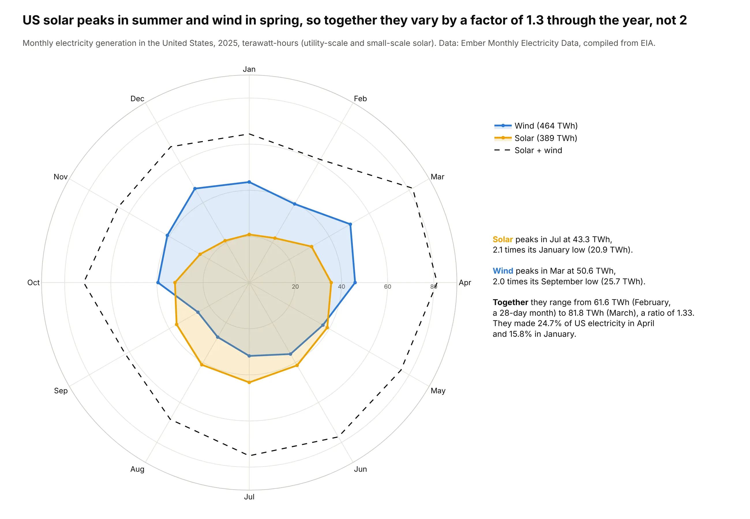
Polar line chart of US monthly generation in 2025: solar peaks in July at 43.3 TWh, wind in March at 50.6 TWh, and the dashed solar plus wind line ranges from 61.6 to 81.8 TWh

Solar peaks in July (43.3 TWh) and wind in March (50.6 TWh), so together they vary by a factor of 1.3 over 2025 rather than about 2. Data: Ember Monthly Electricity Data (from EIA).

Tip: January at the top, months clockwise, and the combined total as an unfilled dashed line.

Get the data from Ember's Monthly Electricity Data (ember-energy.org), United States, 2025
(columns: month, source [Solar, Wind, Total], twh).

Draw a plotly polar line chart: theta = month names (January at the top, clockwise), r = TWh from 0.
Solar and wind filled, solar + wind as a dashed line. Annotate each peak month.

5. California's duck curve on a clock

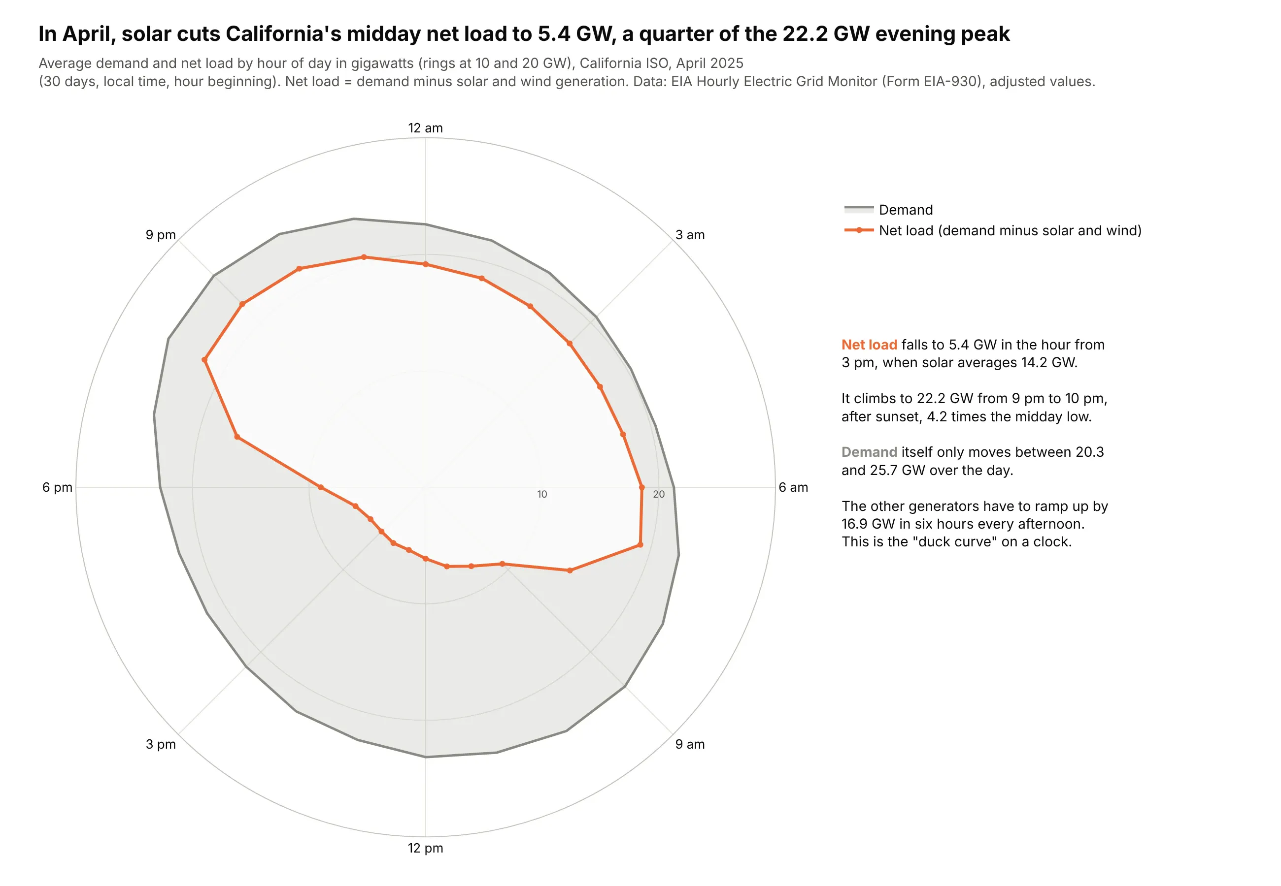
24-hour polar chart of California ISO in April 2025: demand stays between 20.3 and 25.7 GW, while net load after solar and wind falls to 5.4 GW at 3 pm and climbs to 22.2 GW at 9 pm

In April 2025, solar cut California's midday net load to 5.4 GW, a quarter of the 22.2 GW evening peak, so other plants have to add 16.9 GW in six hours every afternoon. Data: EIA Hourly Electric Grid Monitor (Form EIA-930).

Tip: a numeric angle (hour x 15°) with tick labels every three hours, midnight at the top.

Get the data from the EIA Hourly Electric Grid Monitor six-month balance files for 2025 (eia.gov)
for balancing authority CISO (columns: hour, demand_gw, solar_gw, wind_gw), averaged by hour for April.

Draw a plotly polar line chart, theta = hour x 15 degrees (midnight at the top, clockwise),
demand filled gray, net load (demand - solar - wind) in orange. Label 3-hourly ticks.

6. The Atlantic hurricane season

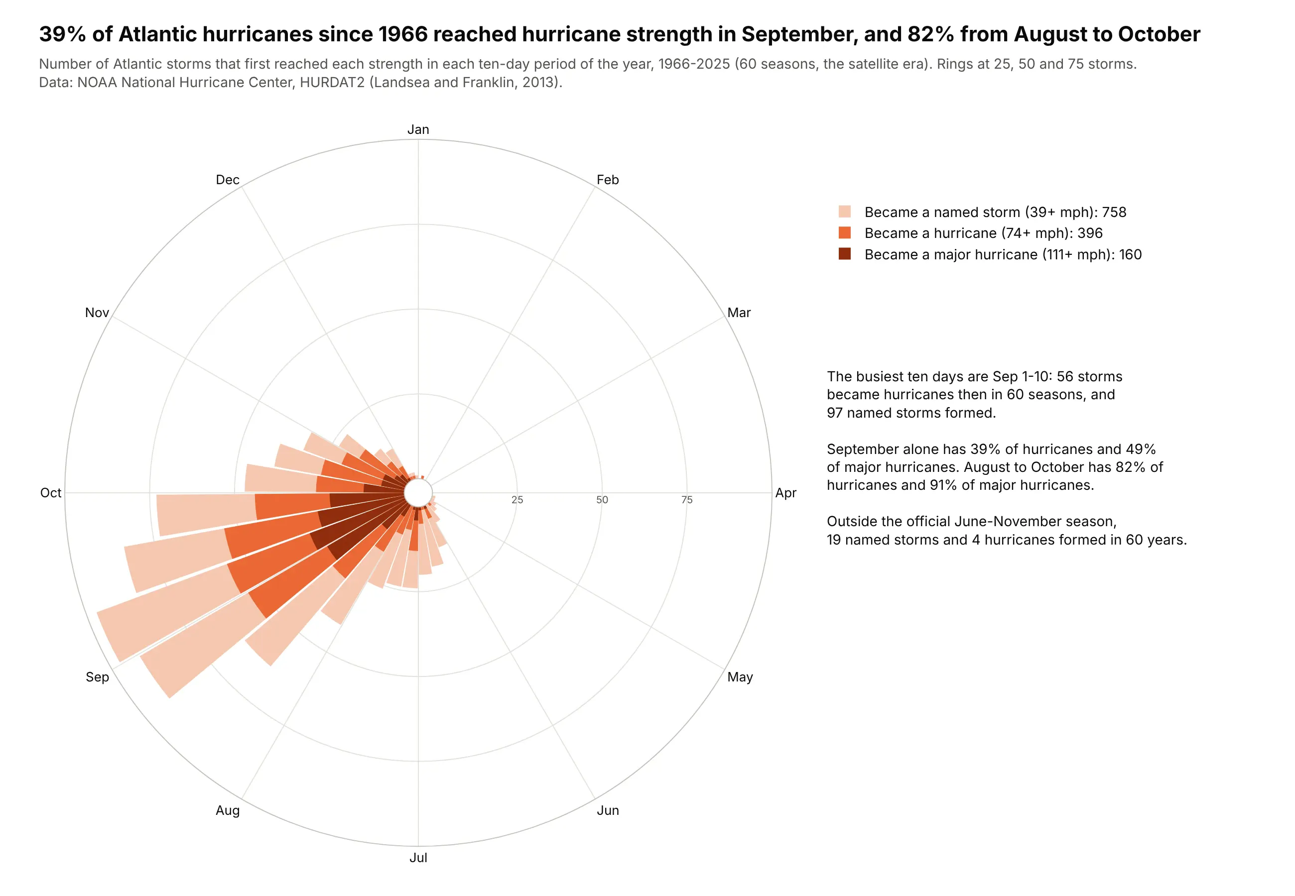
Polar bar chart of Atlantic storms by the ten-day period they reached named storm, hurricane and major hurricane strength, 1966-2025. The bars bulge from August to October, with the most hurricanes in September 1-10

Since 1966, 39% of Atlantic hurricanes reached hurricane strength in September and 82% between August and October, and September 1-10 alone saw 56. Data: NOAA NHC HURDAT2.

Tip: overlaid, not stacked, bars (polar.barmode="overlay"), because every hurricane was a named storm first.

Get the data from NOAA's Atlantic hurricane database HURDAT2 (nhc.noaa.gov/data/hurdat), 1966-2025,
and find the first date each storm reached tropical storm, hurricane and major (96+ kt) strength
(columns: month, part [1-10, 11-20, 21-end], named_storms, hurricanes, major_hurricanes).

Draw a plotly Barpolar with 36 ten-day bins (January at the top), the three counts overlaid
with polar.barmode="overlay", light to dark orange.

7. Six drugmakers' clinical trial fingerprints

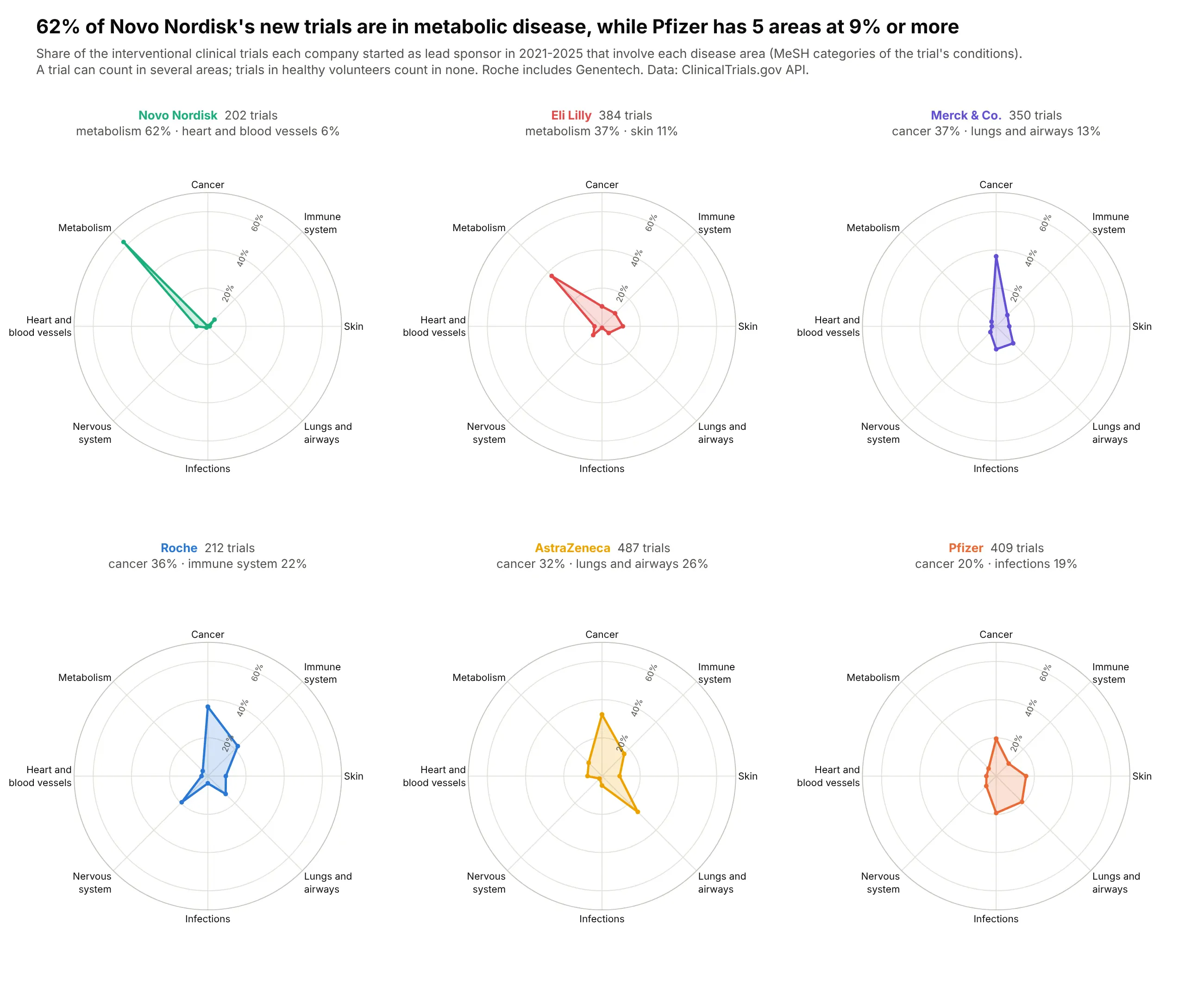
Six radar charts of the share of each company's 2021-2025 clinical trials by disease area. Novo Nordisk's shape is one spike to metabolism (62%), Merck's and Roche's lean to cancer, and Pfizer's spreads across cancer, infections, lungs and skin

62% of the trials Novo Nordisk started since 2021 involve metabolic disease, while Pfizer has five areas at 9% or more. Data: ClinicalTrials.gov API, 2021-2025.

Tip: one shared radial scale across panels, so a spike in one panel compares with the others.

Get the data from the ClinicalTrials.gov API v2, interventional trials started 2021-2025 with lead sponsor
Pfizer, Hoffmann-La Roche or Genentech, AstraZeneca, Eli Lilly, Novo Nordisk or Merck Sharp & Dohme,
tagged by MeSH disease category (columns: company, area, trials, total_trials, pct).

Draw a 2x3 plotly radar grid with a shared 0-70% radial axis, related areas side by side.

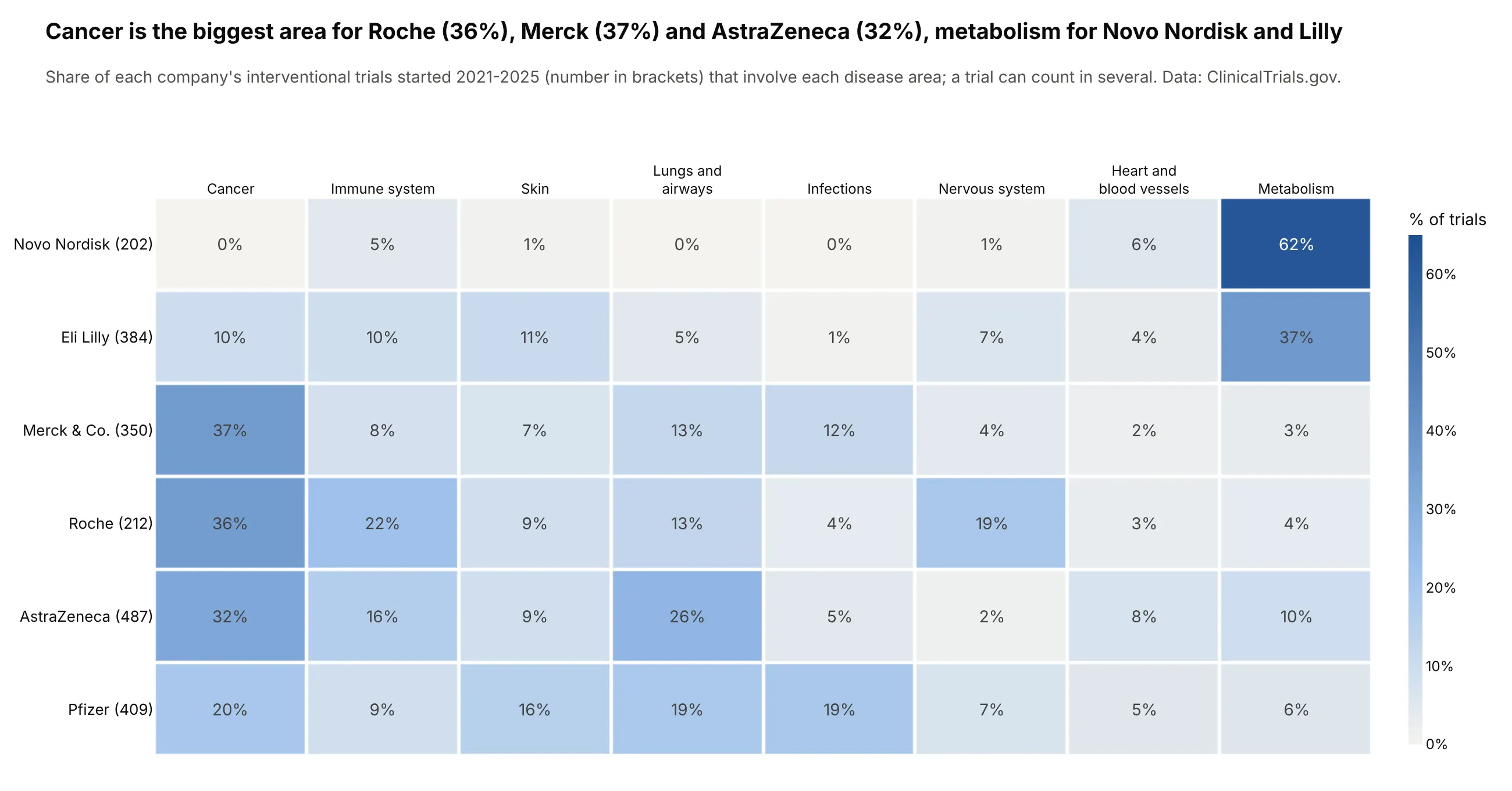
Another way to see it: a heatmap prints all 48 shares.

Heatmap of six drugmakers by eight disease areas: metabolism 62% for Novo Nordisk and 37% for Lilly, cancer 37% for Merck, 36% for Roche and 32% for AstraZeneca

8. State health profiles against the median state

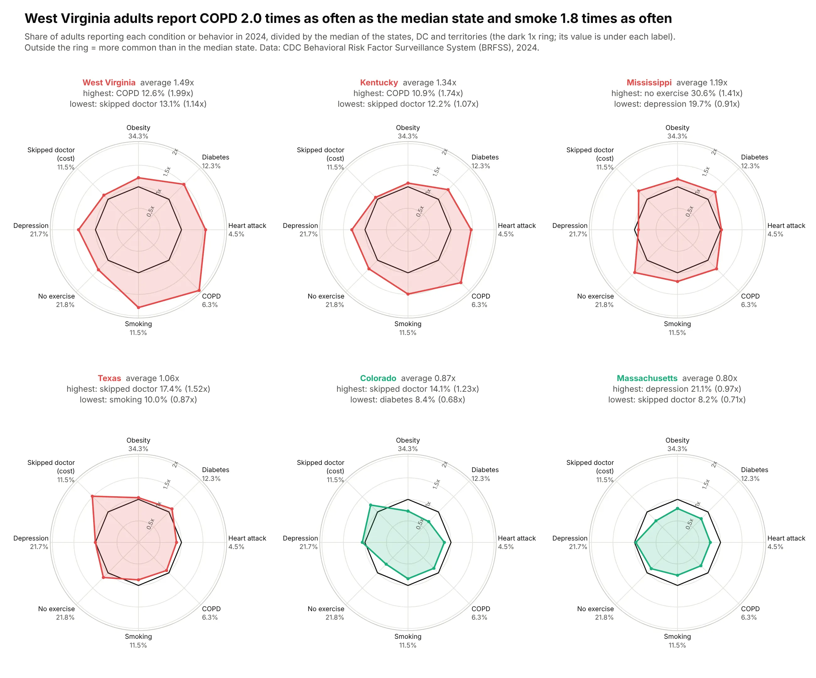
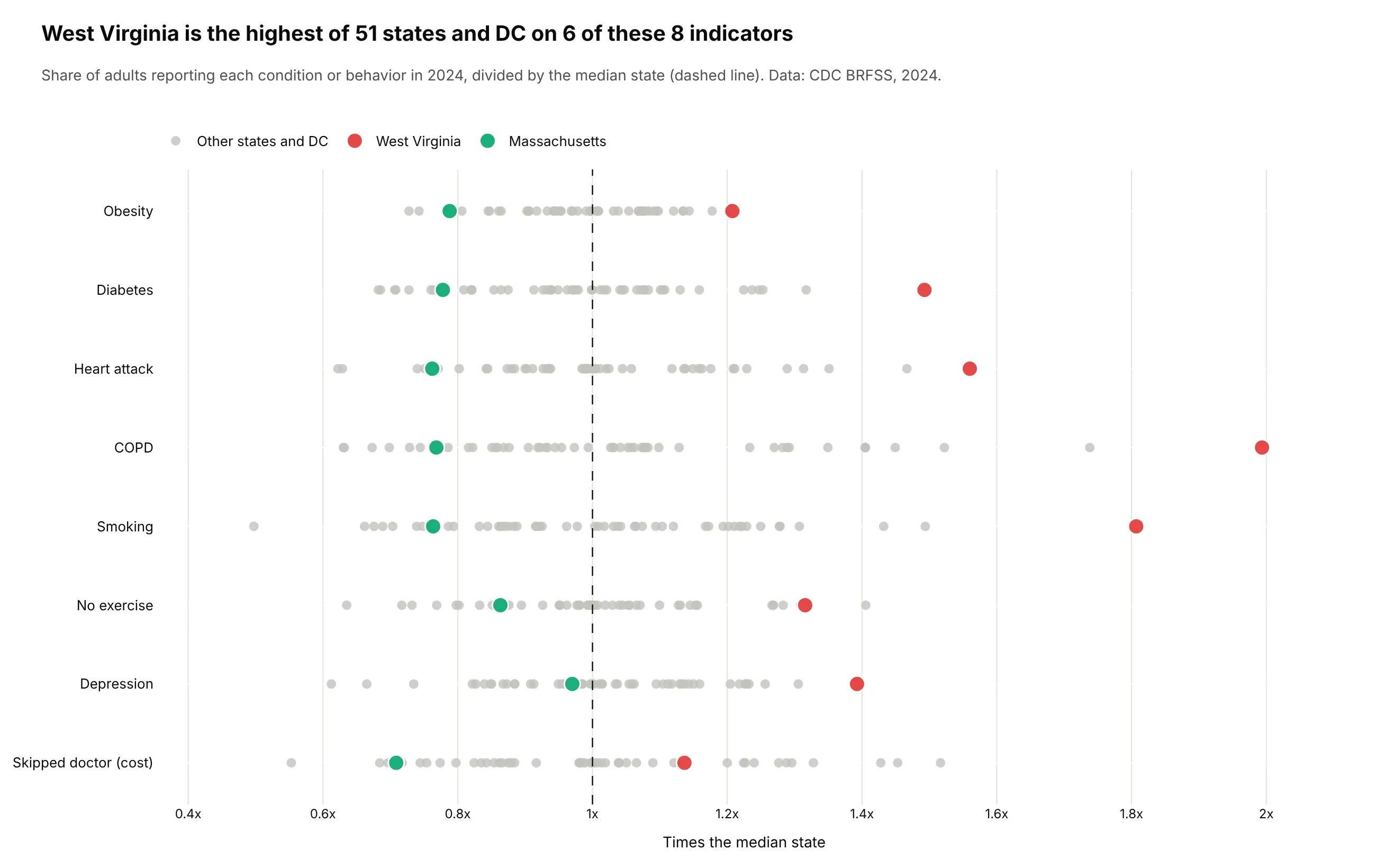
Six radar charts of 2024 BRFSS indicators divided by the median state, with a dark ring at 1x. West Virginia reports COPD at 2.0 times and smoking at 1.8 times the median; Massachusetts sits inside the ring on most indicators

West Virginia adults report COPD at 2.0 times the median state's rate (12.6% vs 6.3%) and smoke 1.8 times as often. Data: CDC Behavioral Risk Factor Surveillance System, 2024.

Tip: a ratio to the benchmark, with the benchmark's raw value under each axis label.

Get the data from CDC BRFSS Prevalence Data (data.cdc.gov dataset dttw-5yxu), 2024, Overall
(columns: state, indicator, pct, us_pct), for obesity, diabetes, heart attack, COPD, smoking,
no exercise, depression and skipped doctor due to cost.

Divide by the US median row. Draw a 2x3 plotly radar grid for WV, KY, MS, TX, CO, MA with a dark ring at 1x
and the median value under each axis label.

Another way to see it: a strip of all 51 states per indicator shows West Virginia is the highest on 6 of 8.

Strip plot of 51 states and DC on eight health indicators as multiples of the median state. West Virginia is the rightmost dot on six, including COPD at 1.99 times and smoking at 1.81 times

9. Sixteen flu seasons on a calendar wheel

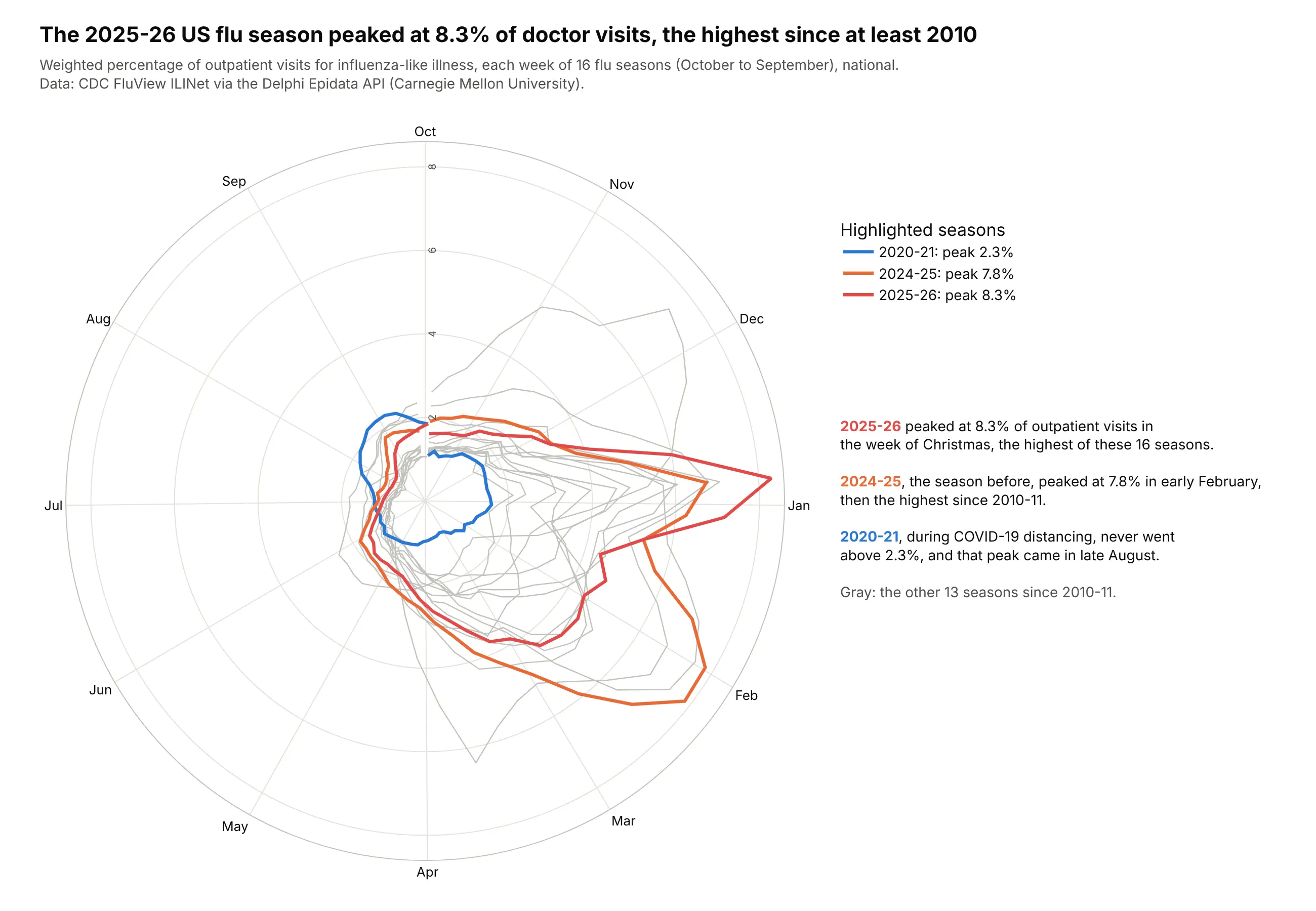
Polar line chart of weekly influenza-like illness for 16 US flu seasons, October at the top. 2025-26 peaks at 8.3% in late December, 2024-25 at 7.8% in early February, and 2020-21 stays below 2.3%

The 2025-26 flu season peaked at 8.3% of outpatient visits in the week of Christmas, the highest of the 16 seasons since 2010-11, a year after 2024-25 set the previous high (7.8%). Data: CDC FluView ILINet via the Delphi Epidata API.

Tip: each week sits at its calendar angle, so month labels mark where months start.

Get the data from CDC FluView ILINet national weighted ILI through the Delphi Epidata API
(api.delphi.cmu.edu/epidata/fluview), seasons 2010-11 to 2025-26
(columns: season, epiweek, week_of_season, wili).

Draw a plotly polar line chart with one line per season, angle = days since October 1,
October at the top, gray lines and color only for 2025-26, 2024-25 and 2020-21.

10. New York's taxis by hour

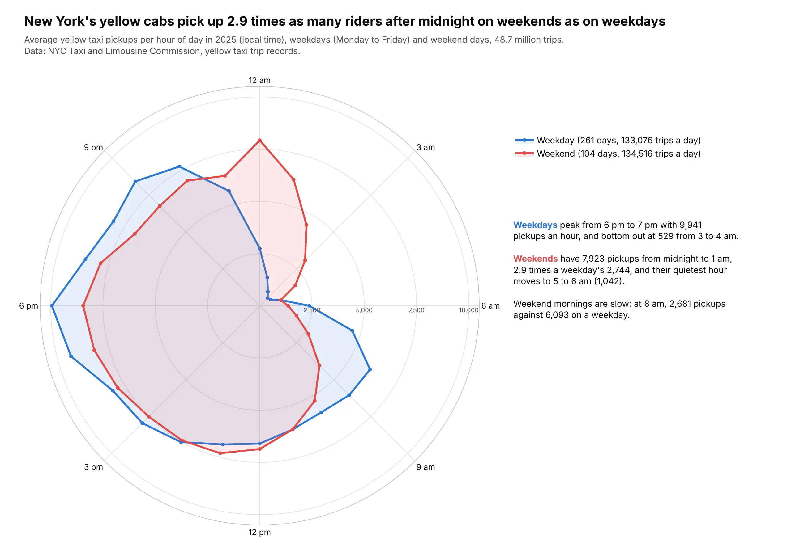
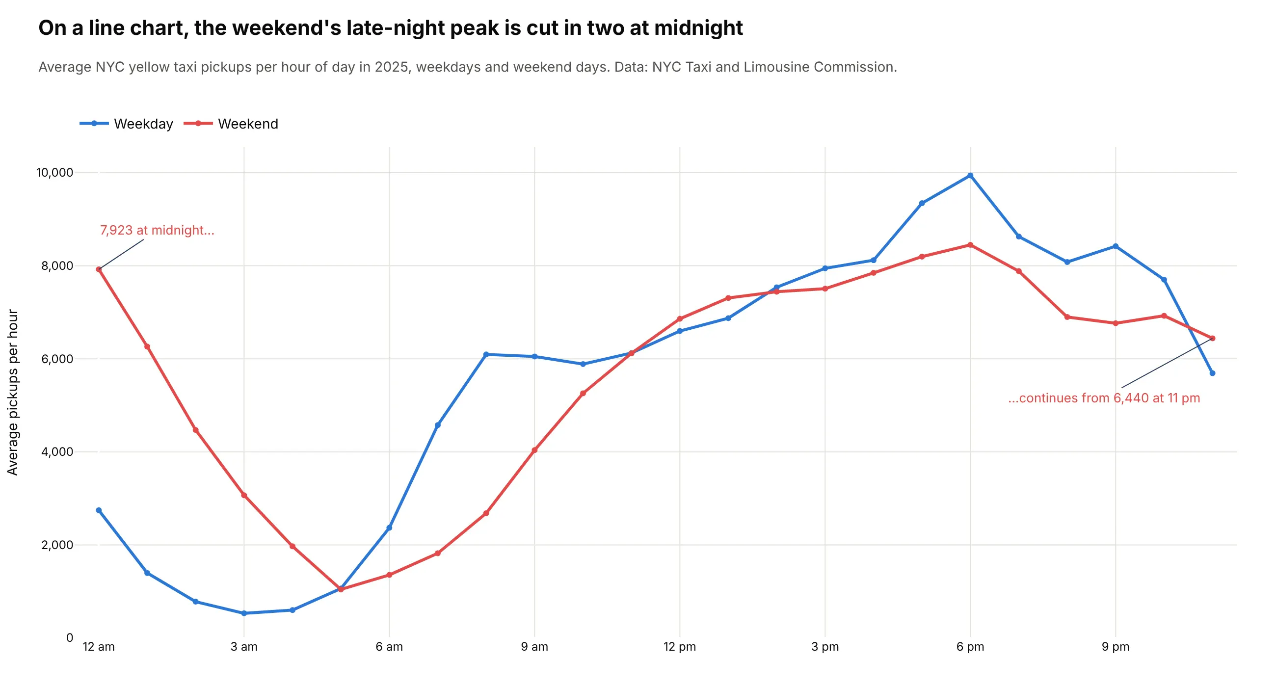
24-hour polar chart of average NYC yellow taxi pickups in 2025. Weekdays peak at 9,941 an hour at 6 pm; weekends bulge after midnight with 7,923 pickups from midnight to 1 am, 2.9 times the weekday's 2,744

Across 48.7 million trips in 2025, yellow cabs picked up 2.9 times as many riders between midnight and 1 am on weekends as on weekdays. Data: NYC Taxi and Limousine Commission trip records.

Tip: on a 24-hour clock, the late-night peak is one bulge, not two ends of an axis.

Get the data from NYC TLC yellow taxi trip records for 2025 (monthly Parquet files, pickup time only)
and count pickups by hour for weekdays and weekends (columns: day_type, hour, trips, days, avg_trips).

Draw a plotly polar line chart, theta = hour x 15 degrees with midnight at the top, one filled line per
day type, and the radial axis from 0.

Another way to see it: on a line chart, the weekend's late-night peak is cut in two at midnight.

Line chart of hourly NYC taxi pickups from midnight to midnight, with the weekend's 7,923 pickups at midnight on the left edge and its 6,440 at 11 pm on the right edge