
Chris Parmer
November 15, 2026
Hertzsprung-Russell Diagrams - A Complete Guide
TL;DR
- A Hertzsprung-Russell (HR) diagram is a scatter plot of stars with their brightness on the y axis (brighter at the top) and their color or temperature on the x axis (hotter on the left), and stars don't fall evenly across it: most lie on a diagonal band called the main sequence, with giants above it and white dwarfs below.
- HR diagrams are also known as H-R diagrams, HRDs and color-magnitude diagrams (CMDs), and when temperature and luminosity are on log axes, as theoretical HR diagrams. They are similar to scatter plots, hexbin plots and 2D histograms when there are too many stars to draw one by one.
- Read them by region: the main sequence is stars fusing hydrogen in their cores (70% of the 222,000 stars within 100 parsecs of the Sun are faint red dwarfs on its lower end), red giants sit above it, and white dwarfs, the faint cores of dead stars, sit below it.
- Astronomers use them to estimate the size of a star from its position, to date star clusters from where the main sequence stops, and to measure how far away a cluster is.
- You can make an HR diagram with Plotly in Python or JavaScript from a scatter trace (go.Scattergl for hundreds of thousands of stars) with the brightness axis reversed.
What is a Hertzsprung-Russell diagram?
This is a Hertzsprung-Russell diagram:
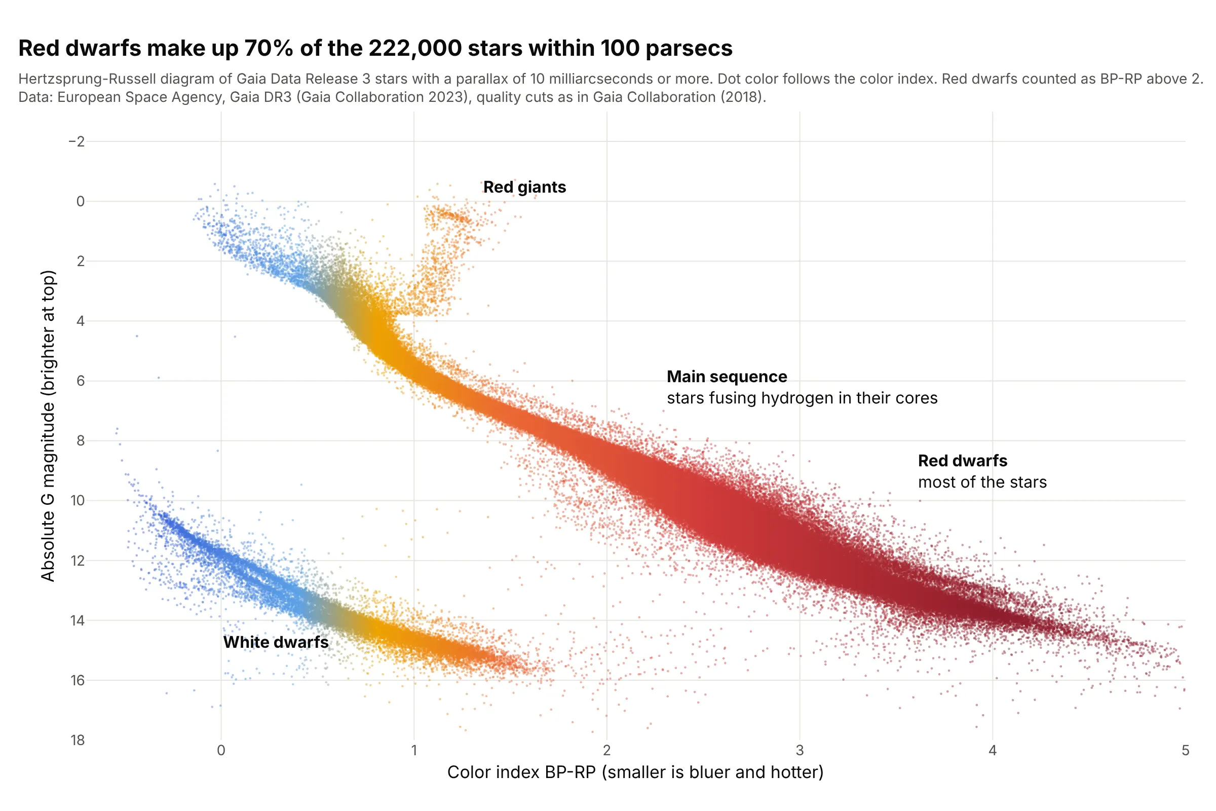
Data: European Space Agency (ESA), Gaia Data Release 3, Gaia Collaboration (2023), stars with a parallax of 10 milliarcseconds or more (within about 100 parsecs, where one parsec is 3.26 light years) and the quality cuts of Gaia Collaboration (2018).
How do you read an HR diagram? In the example above, notice these things:
- Each dot is one of 222,000 stars. Its x position is its color index BP-RP, the difference between its brightness through Gaia's blue and red filters, where a smaller number means bluer and hotter. Its y position is its absolute G magnitude, how bright it would look from a standard distance of 10 parsecs. Magnitudes run backward (a smaller number is brighter), so the axis is reversed to put bright stars at the top.
- The diagonal band is the main sequence, where stars spend most of their lives fusing hydrogen into helium in their cores. Hot, bright stars are at the upper left and cool, faint ones at the lower right.
- Most stars are at the faint end: 154,649 of the 222,000 (70%) have a color index above 2, which makes them red dwarfs.
- The orange group above the main sequence, near a color index of 1.2 and an absolute magnitude of 0.5, is the red giants, stars that have used up the hydrogen in their cores and swelled. Only 552 stars sit in that region.
- The separate band at the lower left is white dwarfs. 15,284 stars (7%) lie in that region, which we defined as more than 8 + 4 times the color index in absolute magnitude.
It's often used for charts like these:
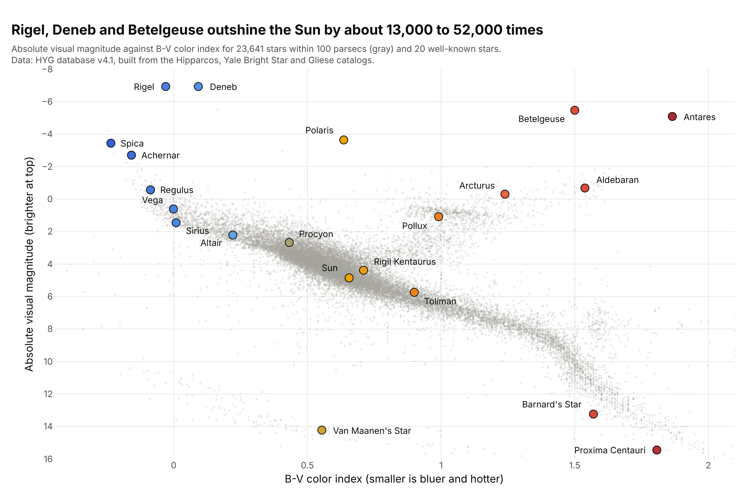
Famous stars (the classic use). A textbook HR diagram labels the stars everyone knows, and shows that Rigel, Deneb and Betelgeuse outshine the Sun by about 13,000 to 52,000 times, while Proxima Centauri, the nearest star, is at the faint end of the main sequence. Data: HYG database v4.1, which combines the Hipparcos, Yale Bright Star and Gliese catalogs (the 3D bar chart guide bins the same stars).
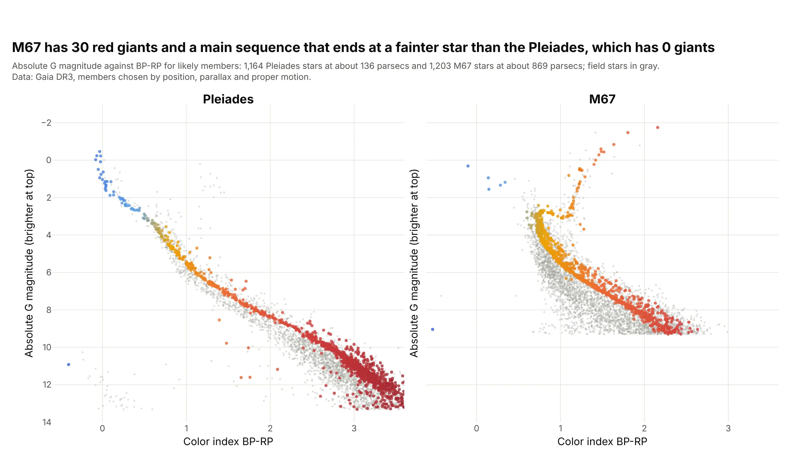
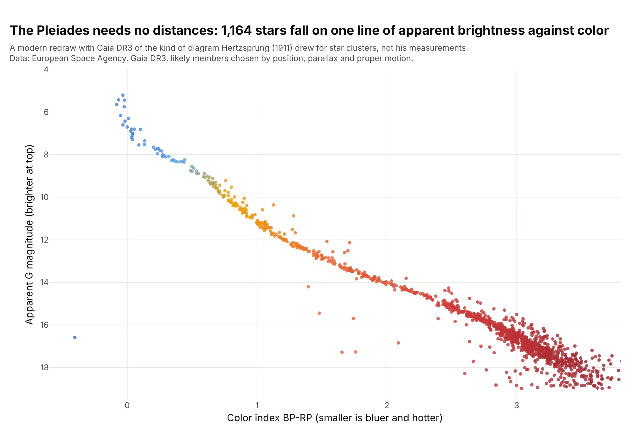
Dating star clusters. The stars of a cluster formed together, so the main sequence of the Pleiades continues up to bright blue stars, while M67 has lost its brighter main sequence stars and shows 30 red giants. The same diagram is how astronomers rank cluster ages. Data: Gaia DR3, 1,164 Pleiades and 1,203 M67 stars picked by position, parallax and proper motion.
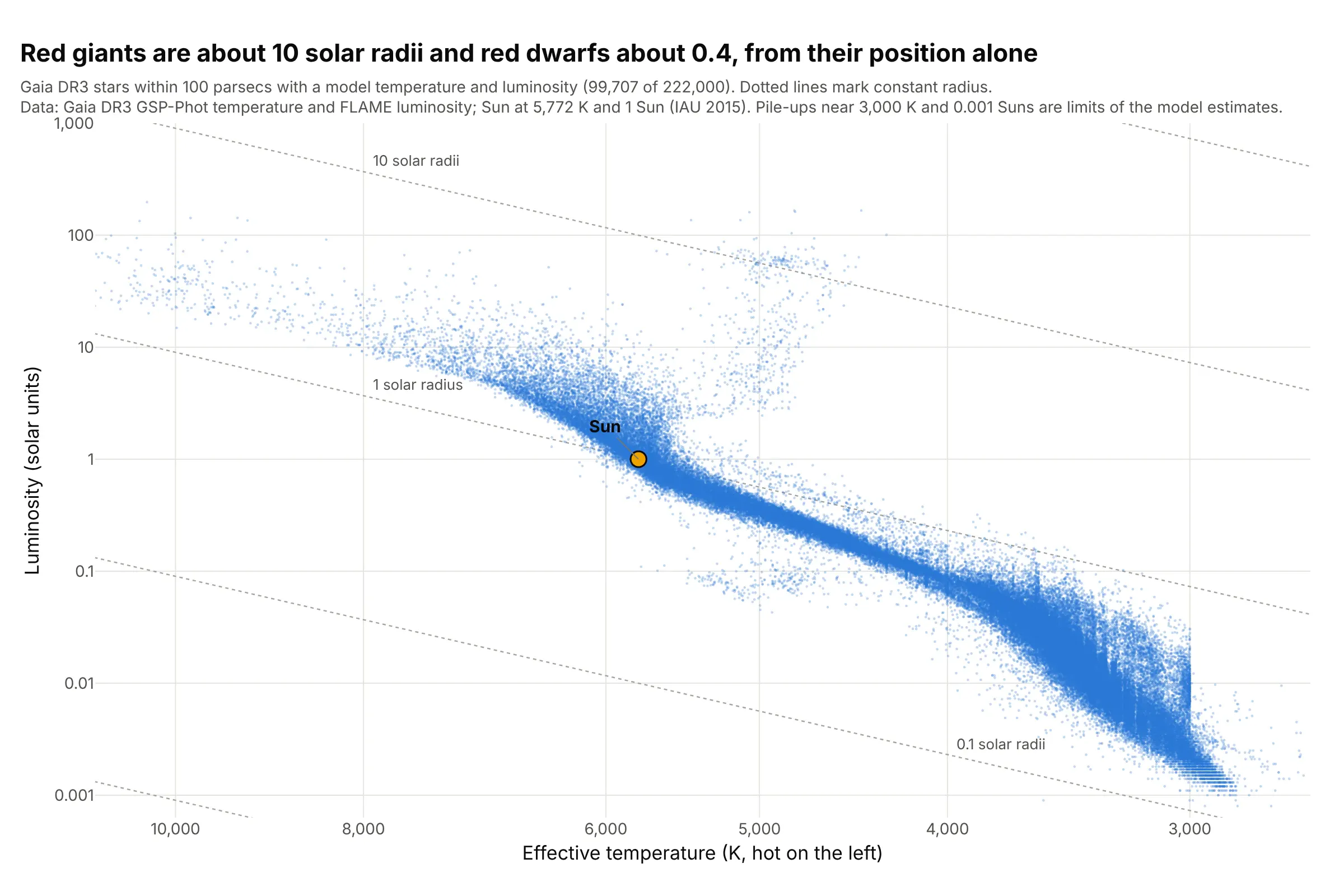
Temperature and luminosity. Theory predicts temperature and luminosity rather than color and magnitude, and the Stefan-Boltzmann law (a star's luminosity is its surface area times the fourth power of its temperature) turns each point into a radius, about 10 solar radii for the red giants and 0.4 for the red dwarfs. Data: Gaia DR3 temperatures and luminosities from the Generalized Stellar Parameterizer from Photometry (GSP-Phot) and the Final Luminosity Age Mass Estimator (FLAME).
How to read an HR diagram from another field
The chart assumes a few ideas from astronomy, and each of them sets one axis or one region.
- Absolute magnitude is how bright a star would look at 10 parsecs. Stars at different distances look brighter or fainter for reasons that have nothing to do with the star, so astronomers convert apparent magnitude m to absolute magnitude M with the star's parallax p (its tiny apparent shift in the sky as Earth orbits the Sun, in milliarcseconds): M = m + 5 log10(p) - 10. A smaller magnitude is a brighter star, and a difference of 5 magnitudes is a factor of 100 in brightness.
- Color index is the difference in a star's magnitude between a blue and a red filter, so it is a measure of temperature that doesn't need a spectrum. Gaia's is BP-RP (its blue and red photometers), and older diagrams use B-V (blue minus visual). Smaller means bluer and hotter, so a color axis that increases to the right already puts hot stars on the left, while a temperature axis has to be reversed.
- Spectral class is the letter astronomers assign to a star from its spectrum, from hottest to coolest O, B, A, F, G, K and M, each split into tenths (the Sun is G2). It was the horizontal axis of the first diagrams (example 3 below).
- Where a star sits follows from its mass and age. On the main sequence mass decides the position (example 4), and when a star runs out of hydrogen in its core it leaves the main sequence for the giant branch, while the leftover core of a low-mass star becomes a white dwarf that only cools.
A short history
Hans Rosenberg published a diagram of the Pleiades in 1910 that plotted the apparent magnitude of its stars against the strength of lines in their spectra, and Ejnar Hertzsprung drew star clusters the same way with a color measure in a 1911 Potsdam publication (the reference Wikipedia gives). In 1913 Henry Norris Russell combined nearby stars with measured distances, stars of the Hyades cluster and several moving groups into the diagram with spectral class on one axis and absolute magnitude on the other, and published it in Popular Astronomy (1914). We couldn't find the original measurements in a public form, so this redraws the idea with modern data: the Pleiades as Hertzsprung drew clusters, with apparent magnitude against color, because every star of a cluster is at about the same distance, which is why a cluster needs no distances at all.
Alternatives to an HR diagram
Here's the same 222,000 stars drawn six ways. Some are better for the question, some worse, some just different:
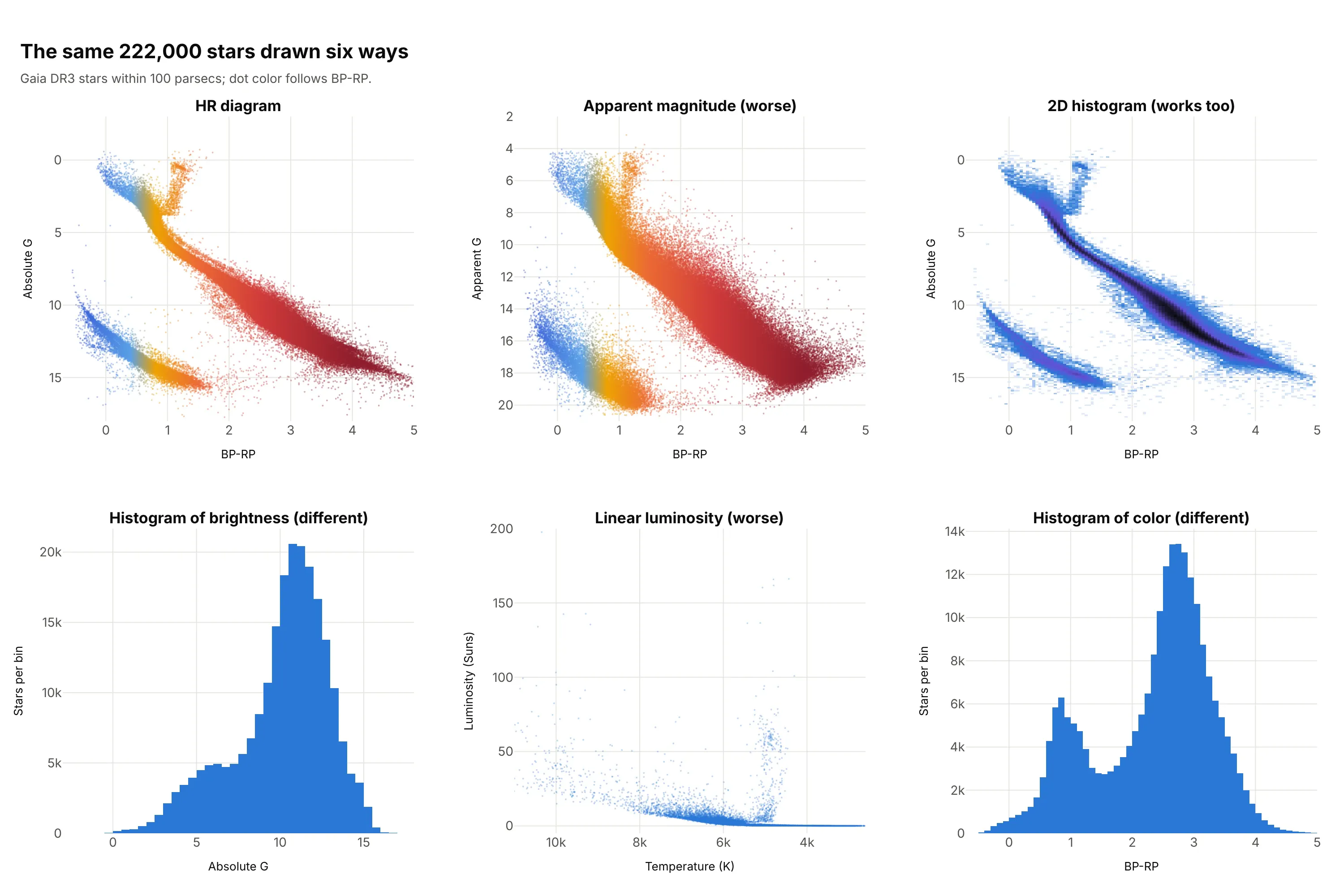
- Apparent magnitude instead of absolute (worse, except in a cluster). Stars at different distances smear the main sequence, because between 10 and 100 parsecs the distance alone changes the apparent magnitude by 5. In a cluster all the stars share a distance, so it works, and it's how the first diagrams were drawn.
- 2D histogram (works too). Counting stars in bins shows where the crowd is, which a scatter plot hides when the dots overlap (example 1 below). A hexbin plot does the same with hexagons.
- Histogram of brightness (different). It is the luminosity function, how many stars there are at each brightness, and it peaks at an absolute magnitude of about 11, but it loses the color, so it can't separate white dwarfs from red dwarfs.
- Linear luminosity (worse). Luminosity spans about five powers of ten in this sample (0.0008 to 198 Suns), so on a linear axis nearly every star is squeezed against zero. Use a log axis.
- Histogram of color (different). It shows two humps, one from Sun-like and hotter stars near 1 and one from the red dwarfs near 3, without the brightness that separates them. For comparison with a scatter plot, the HR diagram is the same idea with a second variable.
How to make a Hertzsprung-Russell diagram
With AI
ChatGPT, Claude Code, GitHub Copilot, Cursor and other AI tools are excellent at writing Plotly code. Name Plotly in the prompt, and say which axis is reversed and how to color the dots:
Make a plotly Hertzsprung-Russell diagram from gaia_100pc.csv (columns: bp_rp, abs_g, the color index and theabsolute G magnitude).- Use go.Scattergl with 2.5 px markers at 0.45 opacity, colored by bp_rp from blue to gold to red.- Reverse the y axis so bright stars are at the top (yaxis autorange reversed). Leave the x axis as it is,because a smaller BP-RP is already bluer and hotter.- Axis titles: "Color index BP-RP (smaller is bluer and hotter)" and "Absolute G magnitude (brighter at top)".- Label the main sequence, the red giants and the white dwarfs. A title that states the takeaway.
With Plotly Studio
Plotly Studio is a product for creating data visualizations and Dash apps and for analyzing data with AI, available as a desktop app or embedded in Dash apps. Ask for an HR diagram the same way:
Show a Hertzsprung-Russell diagram of the Gaia stars within 100 parsecs, color index on x and absolute magnitude on y with bright stars at the top, a dropdown to switch the dots between color index and mass, and a slider for the maximum distance.
Make an HR diagram in Python or JavaScript
This is the code AI tools write under the hood. In Python, a go.Scattergl trace draws the stars, and yaxis_autorange="reversed" puts the bright ones at the top. The absolute magnitude comes from the apparent magnitude and the parallax:
import numpy as npimport pandas as pdimport plotly.graph_objects as gostars = pd.read_csv("gaia_100pc.csv") # g (apparent G magnitude), parallax (mas), bp_rpstars["abs_g"] = stars.g + 5 * np.log10(stars.parallax) - 10 # absolute magnitude, as at 10 parsecsfig = go.Figure(go.Scattergl(x=stars.bp_rp, y=stars.abs_g, mode="markers",marker=dict(size=2.5, opacity=0.45, color=stars.bp_rp, cmin=-0.5, cmax=4.0,colorscale=["#3157d6", "#5aa0e6", "#eda100", "#eb6834", "#d03a3a", "#8f1d2c"]),))fig.update_layout(xaxis_title="Color index BP-RP (smaller is bluer and hotter)",yaxis_title="Absolute G magnitude (brighter at top)",yaxis_autorange="reversed", showlegend=False)fig.show()
For a temperature axis, reverse it too and use log axes: fig.update_xaxes(type="log", autorange="reversed") and fig.update_yaxes(type="log"), with temperature on x and luminosity on y. For a density version, count the stars with np.histogram2d and draw the counts with go.Heatmap, as in example 1 below.
In JavaScript, plotly.js draws the same chart from a scatter trace. This example labels a few well-known stars, with autorange: "reversed" on the y axis:
<div id="chart"></div><script src="https://cdn.plot.ly/plotly-4.1.1.min.js"></script><script>// B-V color index and absolute visual magnitude of well-known stars, from the HYG database v4.1const stars = [["Sun", 0.66, 4.85], ["Sirius", 0.01, 1.45], ["Vega", 0.0, 0.60], ["Procyon", 0.43, 2.67],["Arcturus", 1.24, -0.31], ["Aldebaran", 1.54, -0.68], ["Betelgeuse", 1.50, -5.47], ["Rigel", -0.03, -6.93],["Deneb", 0.09, -6.93], ["Proxima Centauri", 1.81, 15.45], ["Van Maanen's Star", 0.55, 14.22]];Plotly.newPlot("chart", [{x: stars.map(s => s[1]), y: stars.map(s => s[2]), text: stars.map(s => s[0]),mode: "markers+text", textposition: "middle right",marker: {size: 12, color: stars.map(s => s[1]), cmin: -0.3, cmax: 2.0,colorscale: [[0, "#3157d6"], [0.2, "#5aa0e6"], [0.4, "#eda100"], [0.65, "#eb6834"], [0.85, "#d03a3a"], [1, "#8f1d2c"]]}}], {width: 800, height: 560, showlegend: false,xaxis: {title: {text: "B-V color index (smaller is bluer and hotter)"}, range: [-0.4, 2.6], zeroline: false},yaxis: {title: {text: "Absolute visual magnitude (brighter at top)"}, autorange: "reversed", zeroline: false}});</script>
To get the Gaia stars, the Gaia archive answers queries in a language called ADQL (the Astronomical Data Query Language) over a service called the Table Access Protocol (TAP). It returns at most 100,000 rows at a time, so ask for the stars in bands of parallax, as the guide's fetch script does.
Share it
Every Plotly chart has a Share chart button (the cloud icon in its toolbar) that uploads it to Plotly Cloud and gives you a link. Only you can see it until you change its visibility.
For a live app, put the chart in a Dash app and publish it with the Plotly Cloud command-line interface (CLI). Coding agents can run these commands for you:
pip install "dash[cloud]"plotly user loginplotly app publish
If your data has to stay in your own cloud or data center, publish to Dash Enterprise instead.
Dos and don'ts
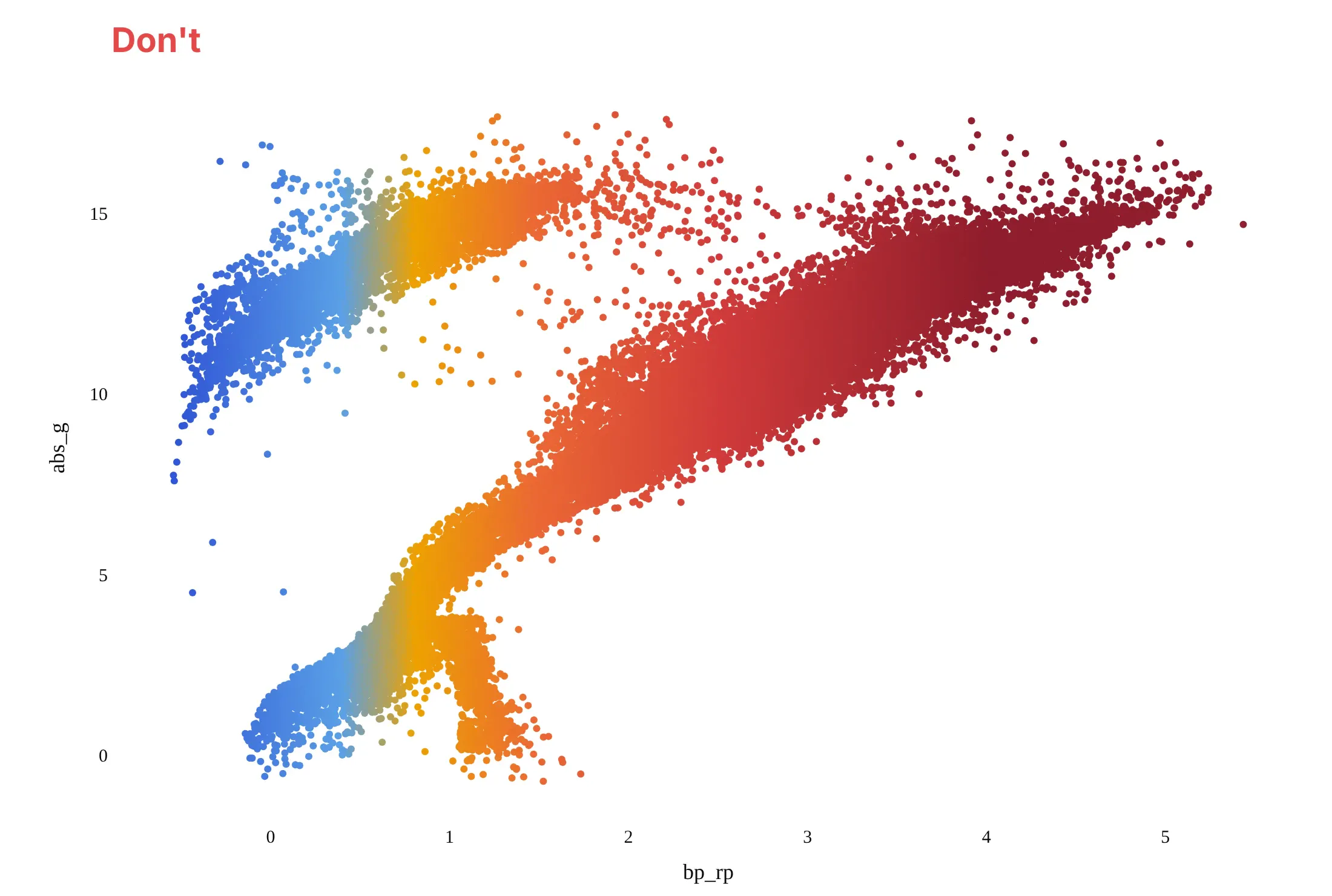
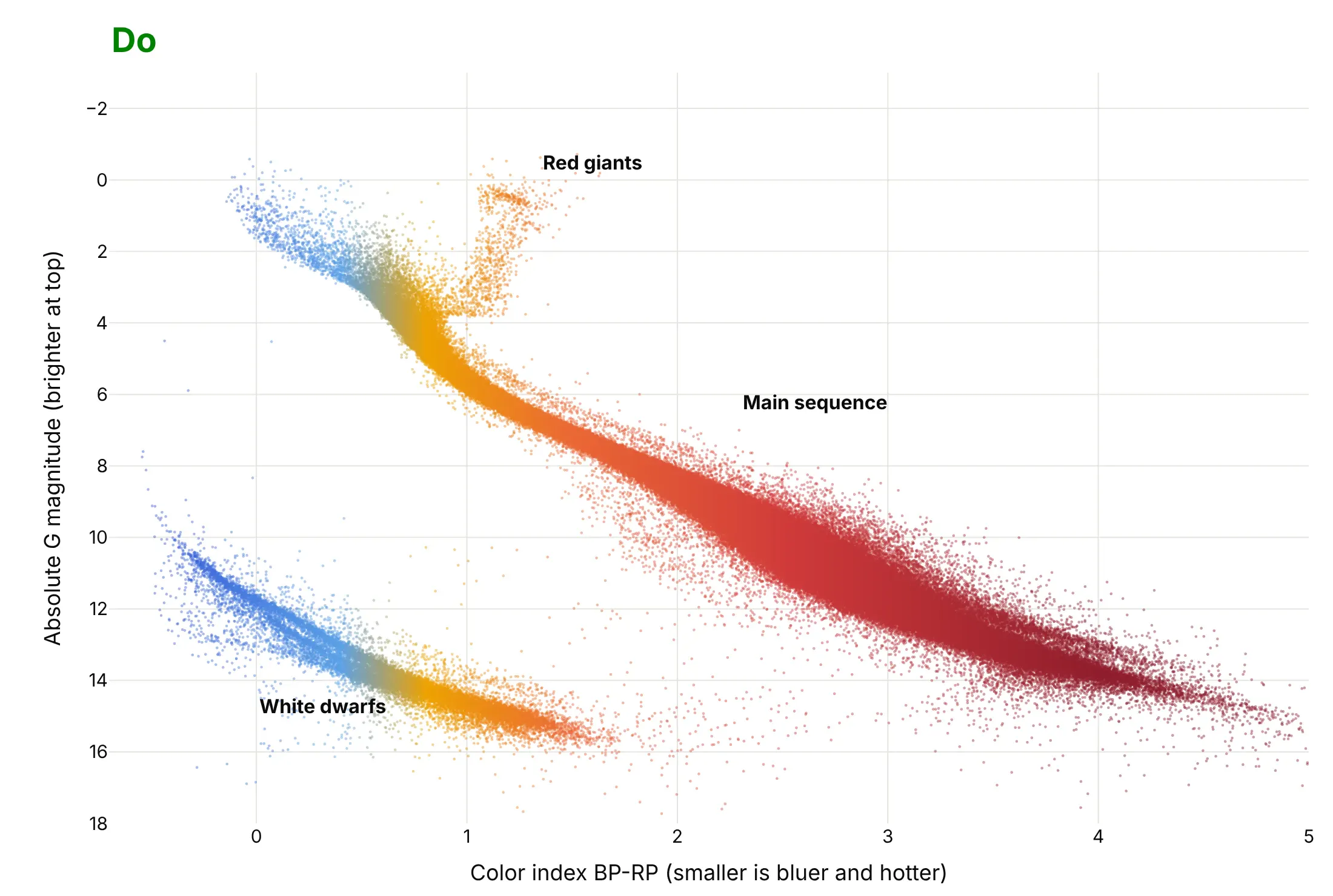
An HR diagram is read by position, so most of the work is getting the axes in the conventional direction and keeping the dots from merging. Here are the Gaia stars both ways, in the same colors.
Don't leave the brightness axis in its natural direction, so that faint stars sit at the top, keep the raw column names bp_rp and abs_g as axis titles, draw large opaque markers that merge into a blob, or use a default serif font:
Do reverse the brightness axis so bright stars are at the top, write the axis titles in words with the direction that matters, use small partly transparent markers so the dense red dwarfs don't hide the rest, and label the main sequence, the giants and the white dwarfs:
Checklist
Do
- Put hot (blue) stars on the left and bright stars at the top, the convention since the first diagrams.
- Use a log axis for luminosity and temperature, and reverse the temperature axis. A color index doesn't need reversing.
- Use absolute magnitude (or luminosity) for stars at different distances, and apparent magnitude only inside one cluster.
- Switch to a 2D histogram or hexbin plot when the dots overlap, and use WebGL (go.Scattergl) above about 10,000 stars.
- Say which catalog, which cuts and which distance limit, because the stars you see depend on how far you look (example 6).
Don't
- Read the density of dots as the density of stars in space. A catalog that reaches farther for bright stars shows too many giants.
- Treat the color of the dots as a physical star color. It only follows the color index.
- Call a chart an HR diagram without saying whether the x axis is spectral class, color index or temperature.
More Hertzsprung-Russell diagram examples
Six more HR diagrams built from real public data, each with its source, a tip and a prompt to rebuild it.
1. Counting stars instead of drawing them
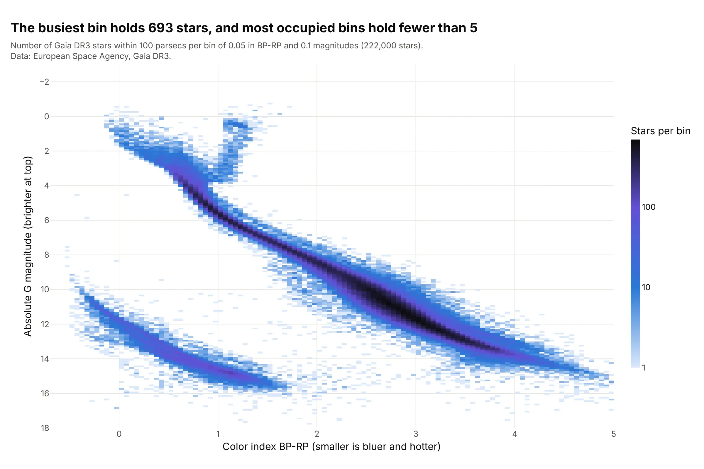
With 222,000 dots the red dwarfs merge into one mass, while binned counts show the busiest bin holds 693 stars and the median occupied bin holds 4. The log color scale keeps the giants and white dwarfs visible next to the crowd. This is the same plot a hexbin or 2D histogram guide describes. Data: ESA Gaia DR3.
Tip: put the counts on a log color scale, or the main sequence turns into one dark stripe and everything else vanishes.
Get the data from the Gaia Data Release 3 catalog (gaiadr3.gaia_source) through a Table Access Protocol service such ashttps://gaia.ari.uni-heidelberg.de/tap: stars with parallax >= 10 mas, parallax_over_error > 10 and ruwe < 1.4,in bands of parallax because a query returns at most 100,000 rows (columns: g, parallax, bp_rp).Compute absolute G = g + 5*log10(parallax) - 10 and build a plotly 2D histogram of bp_rp (bins of 0.05) against absolute G(bins of 0.1) with np.histogram2d and go.Heatmap, log10 counts, empty bins white, the y axis reversed.
2. White dwarfs
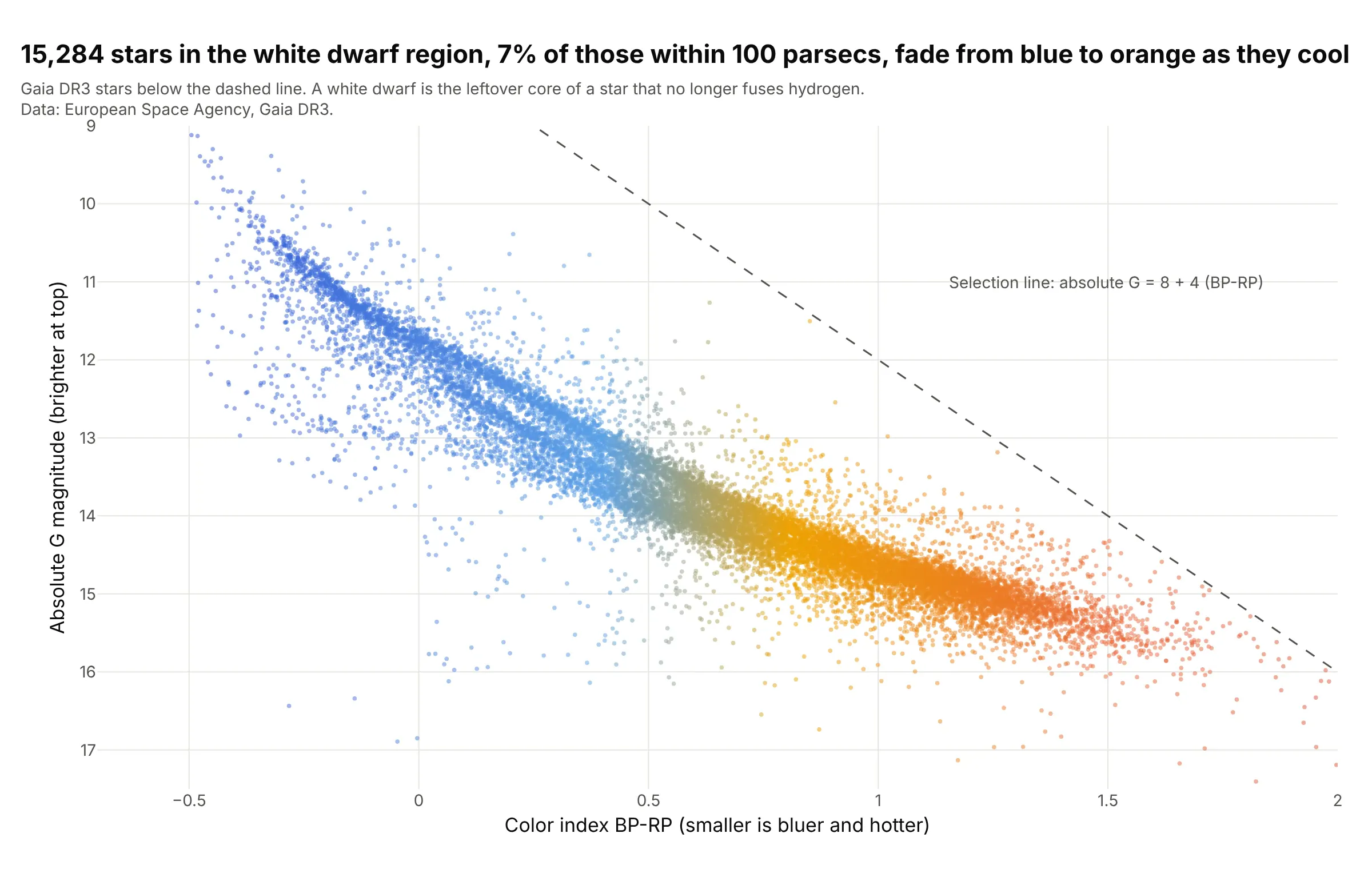
The 15,284 stars below the dashed line (7% of the sample) fade from blue to orange as they cool, tracing the cooling sequence of white dwarfs, the cores left behind when stars like the Sun run out of fuel. Near a color index of 0 they split into two bands. Data: ESA Gaia DR3.
Tip: zoom the axes to the region instead of plotting everything, so the structure inside it is visible.
Get the data from the Gaia Data Release 3 catalog (gaiadr3.gaia_source): stars with parallax >= 10 mas,parallax_over_error > 10 and ruwe < 1.4 (columns: g, parallax, bp_rp).Compute absolute G = g + 5*log10(parallax) - 10, keep stars with absolute G > 8 + 4*bp_rp, and build a plotly scatterof bp_rp (-0.7 to 2) against absolute G (9 to 17.5, reversed), 4 px markers at 0.5 opacity colored by bp_rp, and adashed line for the selection.
3. Russell's axes: spectral class
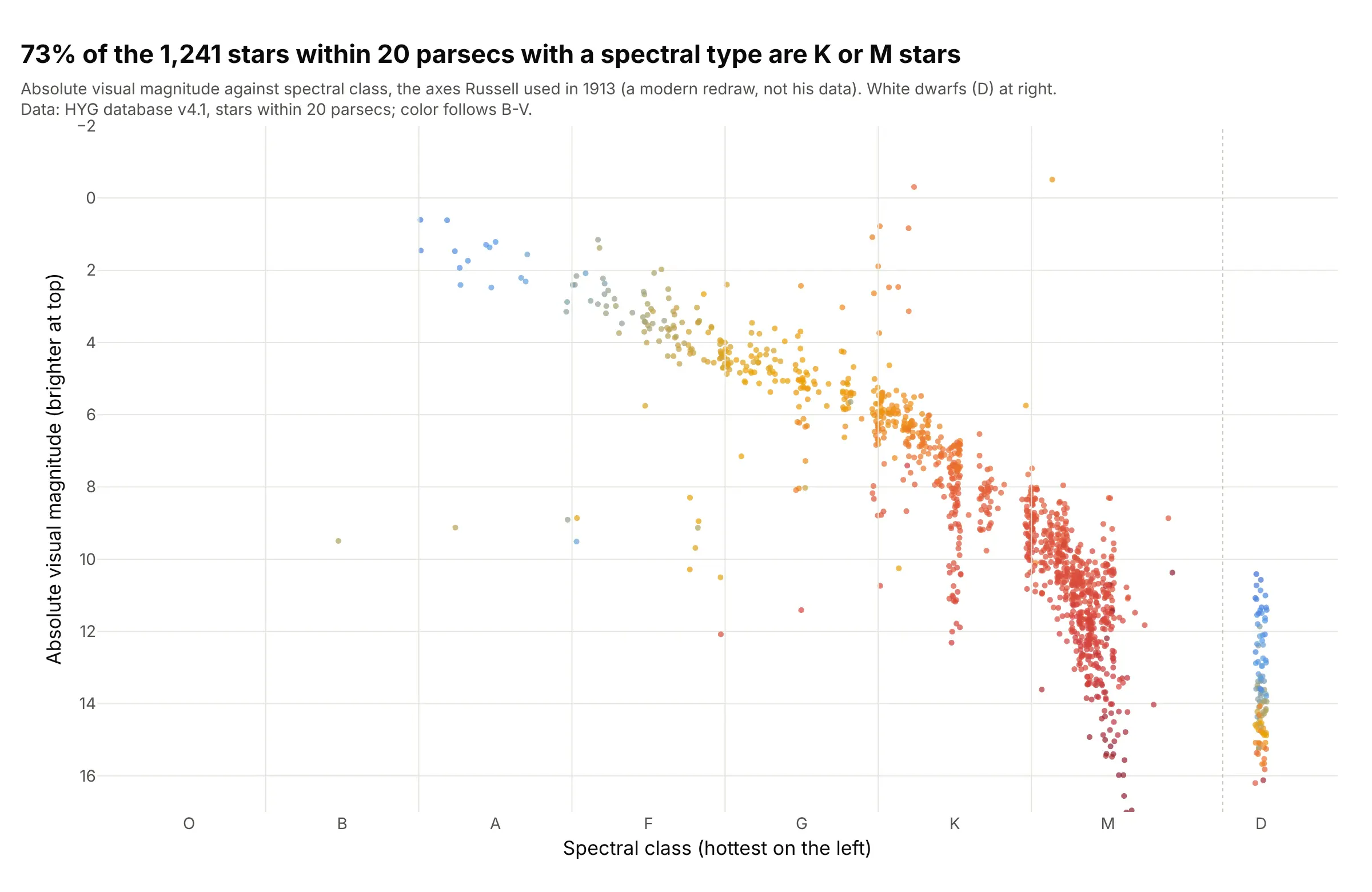
Russell's 1913 diagram had spectral class on x. Drawn with the stars within 20 parsecs, 73% of the 1,241 with a class are K or M stars, and 100 are white dwarfs (the column at the right). This is a modern redraw, not his data. Data: HYG database v4.1.
Tip: place each star at its class letter plus its digit (G2 is 4.2) with a little horizontal jitter, so a categorical axis doesn't stack the dots in one line.
Get the data from the HYG star database v4.1 (https://github.com/astronexus/HYG-Database, file hyg/CURRENT/hygdata_v41.csv)(columns: dist, absmag, ci, spect).Keep stars within 20 parsecs, parse spect into a class letter (O, B, A, F, G, K, M) and a digit, and build a plotly scatterof class position (letter index plus digit/10, white dwarfs starting with D in their own column) against absmag(reversed), jittered by 0.04, colored by ci, with the letters as x tick labels.
4. Mass sets the position on the main sequence
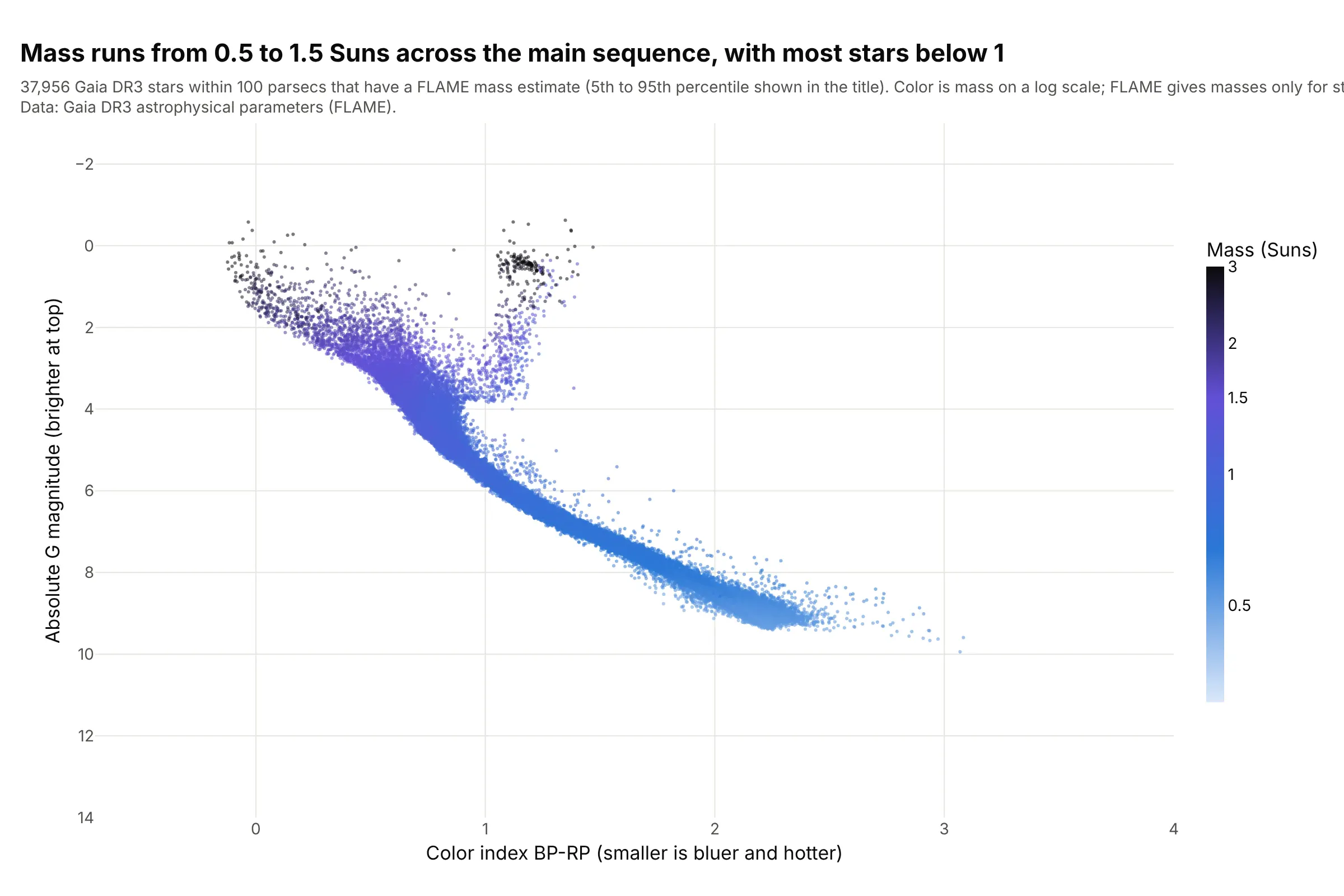
Colored by mass, the main sequence is ordered: the 5th to 95th percentile of the masses runs from 0.54 to 1.46 Suns, and the median star is 0.85 Suns. The most massive stars are at the upper left and the giants are heavy ones too. Data: Gaia DR3 FLAME masses, available for 37,956 of the 222,000 stars.
Tip: color by the log of the mass, with the colorbar labeled in Suns, because a linear scale gives all the faint stars the same color.
Get the data from the Gaia Data Release 3 catalog: gaiadr3.gaia_source joined to gaiadr3.astrophysical_parameterson source_id, stars with parallax >= 10 mas, parallax_over_error > 10 and ruwe < 1.4 (columns: g, parallax, bp_rp,mass_flame).Keep stars with a mass_flame, and build a plotly HR diagram (bp_rp against absolute G, y reversed) colored bylog10(mass_flame) with a colorbar ticked at 0.5, 1, 1.5, 2 and 3 Suns.
5. Stars with planets
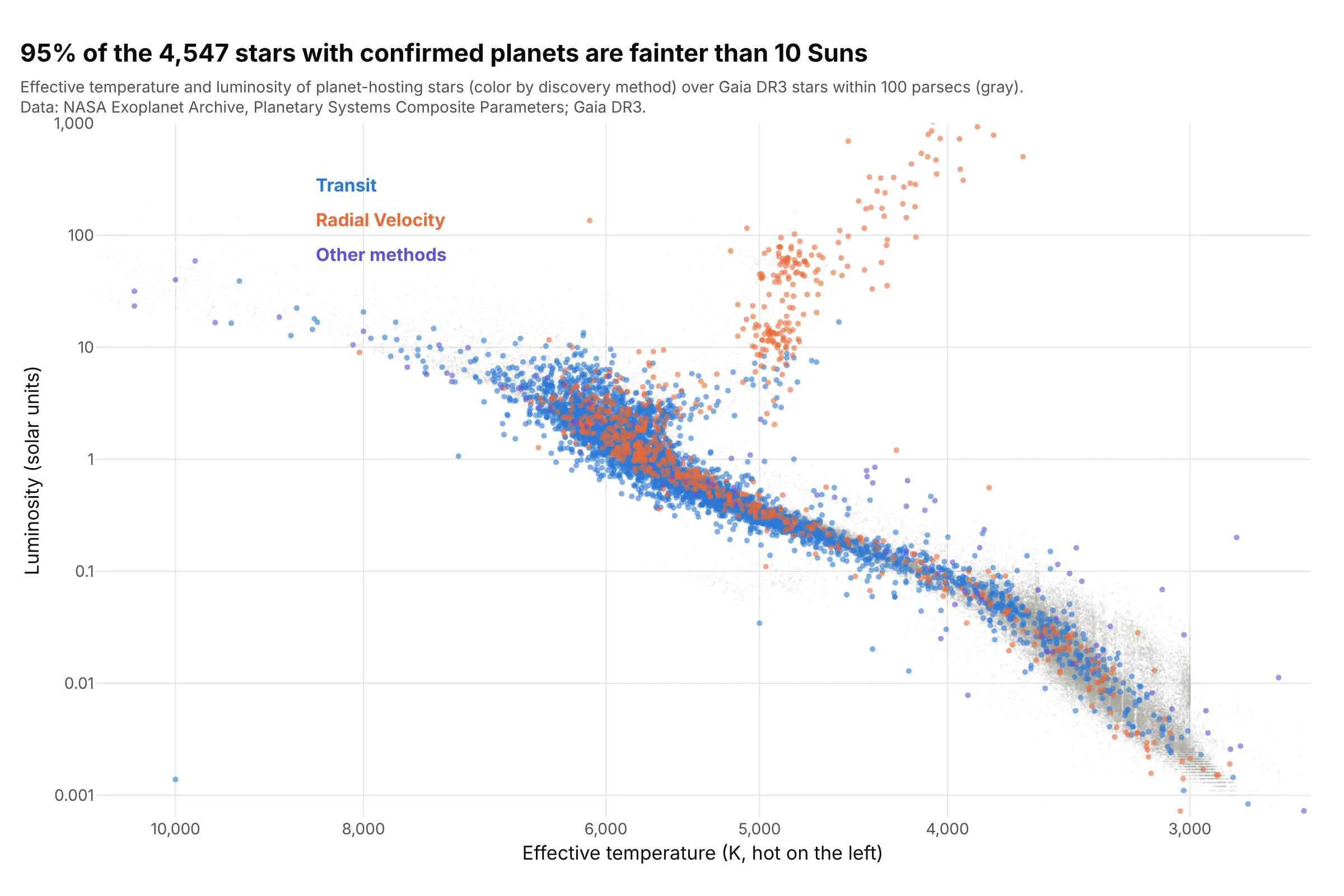
Of the 4,547 stars with a measured temperature and luminosity in the NASA Exoplanet Archive, 95% are fainter than 10 Suns, and 3,628 were found by the transit method. The orange giants at the top right were found by radial velocity. Data: NASA Exoplanet Archive, Planetary Systems Composite Parameters, over Gaia DR3 stars.
Tip: draw the background field first in a light gray, so the colored hosts show where the planet search has looked.
Get the data from the NASA Exoplanet Archive Table Access Protocol service(https://exoplanetarchive.ipac.caltech.edu/TAP/sync), table pscomppars:select hostname, st_teff, st_lum, discoverymethod from pscomppars (st_lum is log10 of the luminosity in Suns).Build a plotly scatter of st_teff (log axis, reversed, hot on the left) against 10**st_lum (log axis), colored bydiscoverymethod for Transit, Radial Velocity and everything else, with the Gaia stars as a light gray background.
6. What you see depends on how far you look
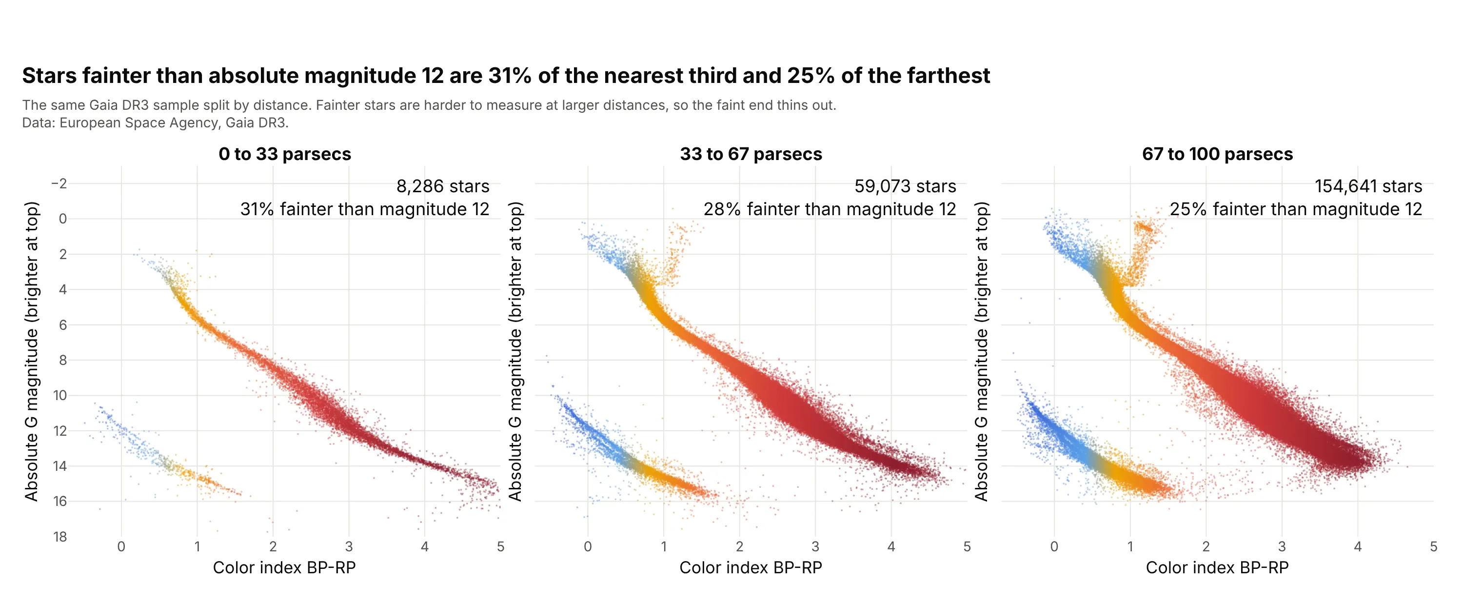
Split by distance, stars fainter than absolute magnitude 12 are 31% of the nearest 8,286 and 25% of the farthest 154,641, and the giant region holds 3 stars in the nearest shell against 447 in the farthest, because giants are rare and the volume grows with distance. The stars are the same sample, but fainter stars are harder to measure at larger distances. Data: ESA Gaia DR3.
Tip: use the same axes in every panel, so the shells can be compared by eye, and put the star count in each panel.
Get the data from the Gaia Data Release 3 catalog (gaiadr3.gaia_source): stars with parallax >= 10 mas,parallax_over_error > 10 and ruwe < 1.4 (columns: g, parallax, bp_rp).Build three plotly HR diagrams side by side with make_subplots and shared y axes for the distance shells 0 to 33,33 to 67 and 67 to 100 parsecs (distance = 1000 / parallax), each with its star count and the share fainter thanabsolute magnitude 12 in the corner.
FAQ
Options to customize
An HR diagram in Plotly is a scatter trace (or a heatmap of counts) with two axes set the way astronomers read them, so these are the options that matter most. The full lists are in the scattergl trace reference, the scatter trace reference and the heatmap reference.
- go.Scattergl or render_mode="webgl": WebGL markers for tens of thousands of stars or more.
- yaxis.autorange="reversed": puts bright stars (small magnitudes) at the top; use it on the x axis for a temperature axis so hot stars are on the left.
- xaxis.type="log", yaxis.type="log": log axes for temperature and luminosity.
- marker.color, marker.colorscale, marker.cmin, marker.cmax: color the dots by color index, mass or distance, with the scale fixed so panels match.
- marker.size, marker.opacity: 2 to 3 px at 0.4 to 0.5 opacity for hundreds of thousands of stars, so the dense red dwarfs don't hide the rest.
- go.Heatmap or go.Histogram2d: counts per bin on a log color scale, for crowded samples.
- marker.colorbar.tickvals, ticktext: label a log color scale in real units (Suns, stars per bin).
- add_annotation with ax, ay: labels for the main sequence, giants, white dwarfs and named stars.
- add_trace with mode="lines": lines of constant radius, an isochrone or a selection boundary.
- customdata and hovertemplate: a star's name, distance or catalog ID on hover.
- make_subplots with shared_yaxes=True: clusters or distance shells side by side on the same axes.
- xaxis.tickvals and ticktext: spectral class letters at their positions for Russell's form.