Density Maps - A Complete Guide

TL;DR

• A density map puts a soft blob of color on a map around every point and adds the blobs up, so places with many points nearby turn dark. It shows where events cluster when there are too many to draw as dots.
• Density maps are also known as heat maps, kernel density maps and density heatmaps, and are similar to hexbin maps, choropleth maps and bubble maps.
• The radius of each blob and the weight of each point decide what the map shows, so the same data can look like a few hot spots or one dark mass. This guide shows how to set both.
• You can make a density map with Plotly in one line of code with px.density_map, which draws a densitymap trace on a MapLibre base map with no access token. It replaced px.density_mapbox, which Plotly 7 removed.

What is a density map?

Density maps look like this:

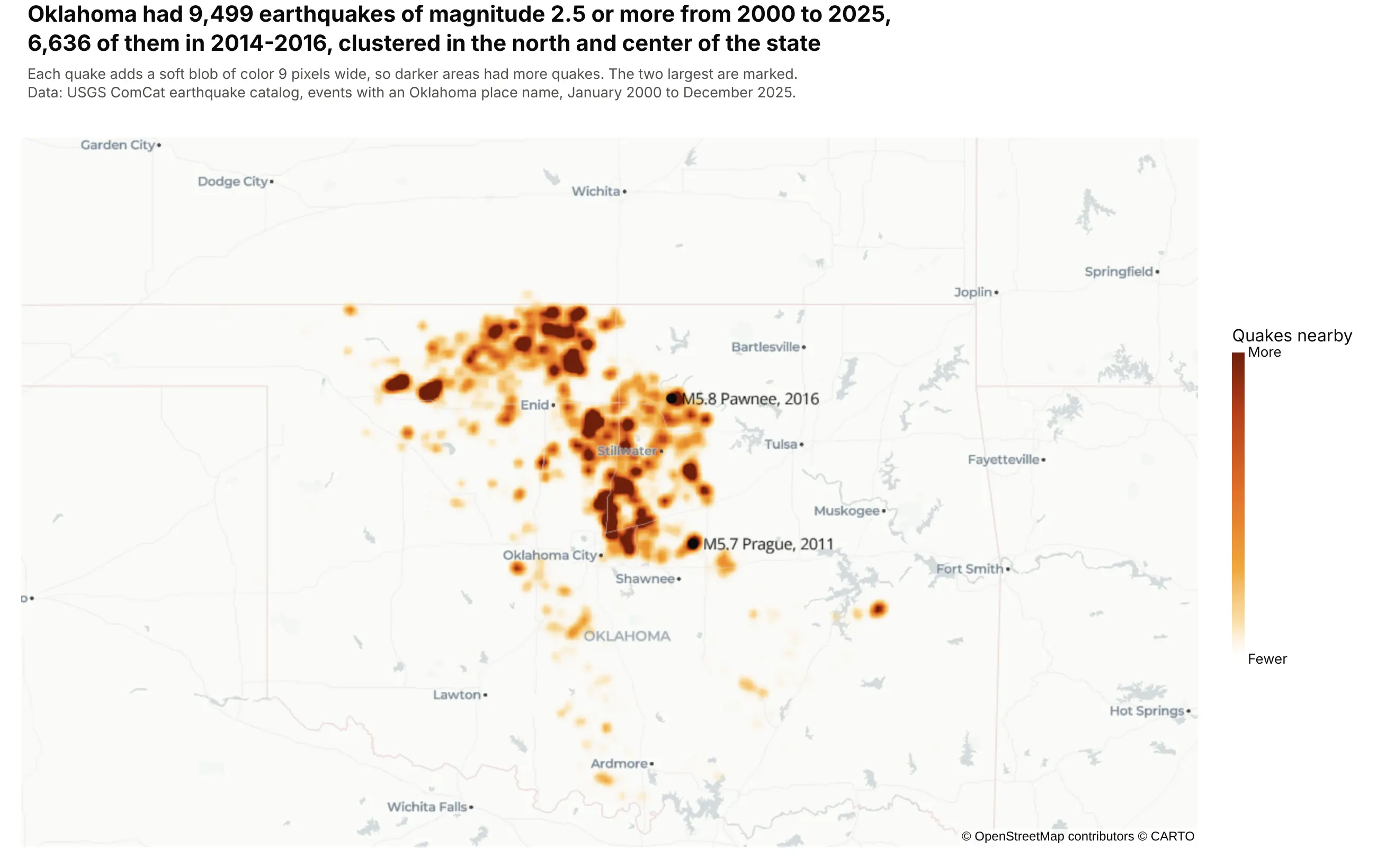
Data: USGS ComCat earthquake catalog, 2000 to 2025.

How do you read a density map? In the example above, notice these things:

• Each quake adds a soft blob of color 9 pixels wide around its epicenter, and the blobs add up, so the color shows how many quakes happened nearby, not the strength of any one quake.
• The colors have no unit. Here each quake adds a twelfth of the full color, so the darkest spots have roughly a dozen or more quakes close together, and the color bar only says fewer or more.
• The darkest areas are in the north and center of the state. Grant County, on the Kansas line, had 1,682 of the 9,499 quakes, more than any other county.
• The map adds up 26 years, and the quakes are not spread evenly over them: 6,636 struck in 2014-2016 and only 35 before 2009. Seismologists link the increase to wastewater injected deep underground by the oil and gas industry (Keranen et al. 2014).
• The two marked quakes are the largest, an M5.8 near Pawnee in 2016 and an M5.7 near Prague in 2011. Big quakes and frequent quakes are different questions, and this map answers the second.

It's often used for charts like these:

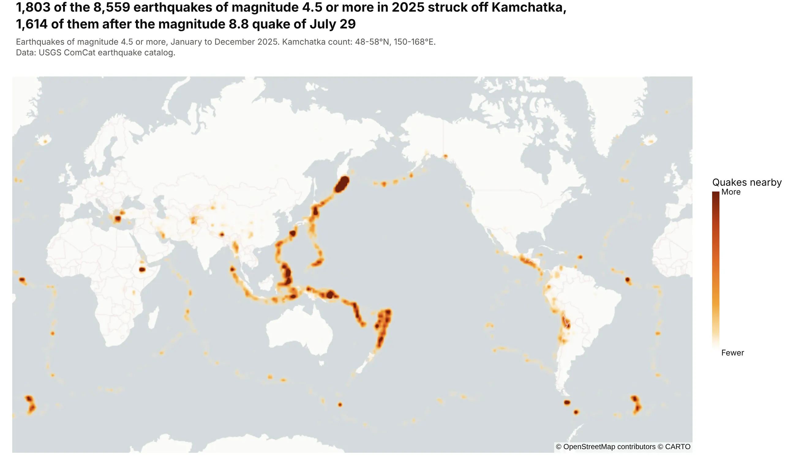
Earthquakes, the classic dataset. 1,803 of the 8,559 earthquakes of magnitude 4.5 or more in 2025 struck off Kamchatka, 1,614 of them after the magnitude 8.8 quake of July 29. Data: USGS ComCat earthquake catalog.

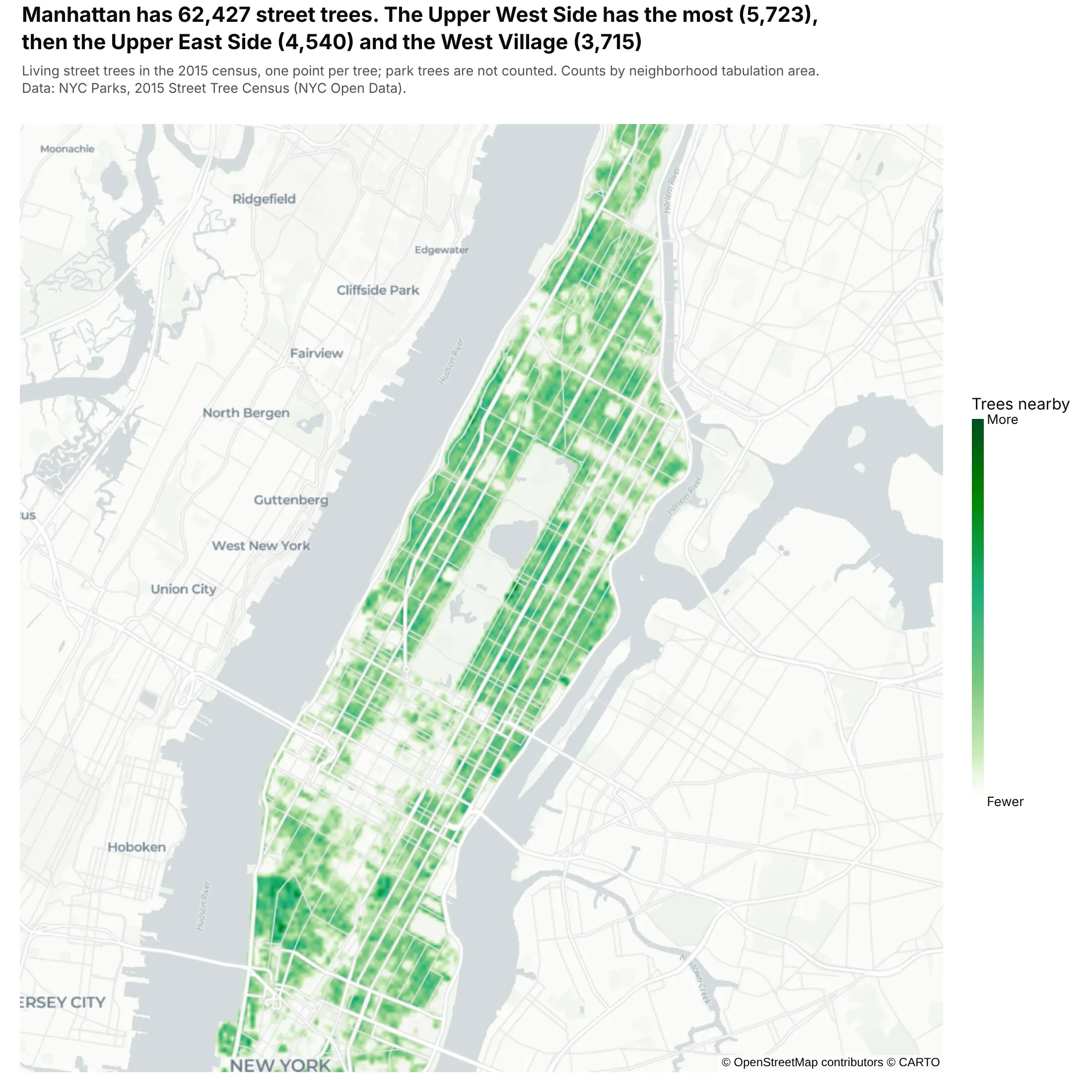
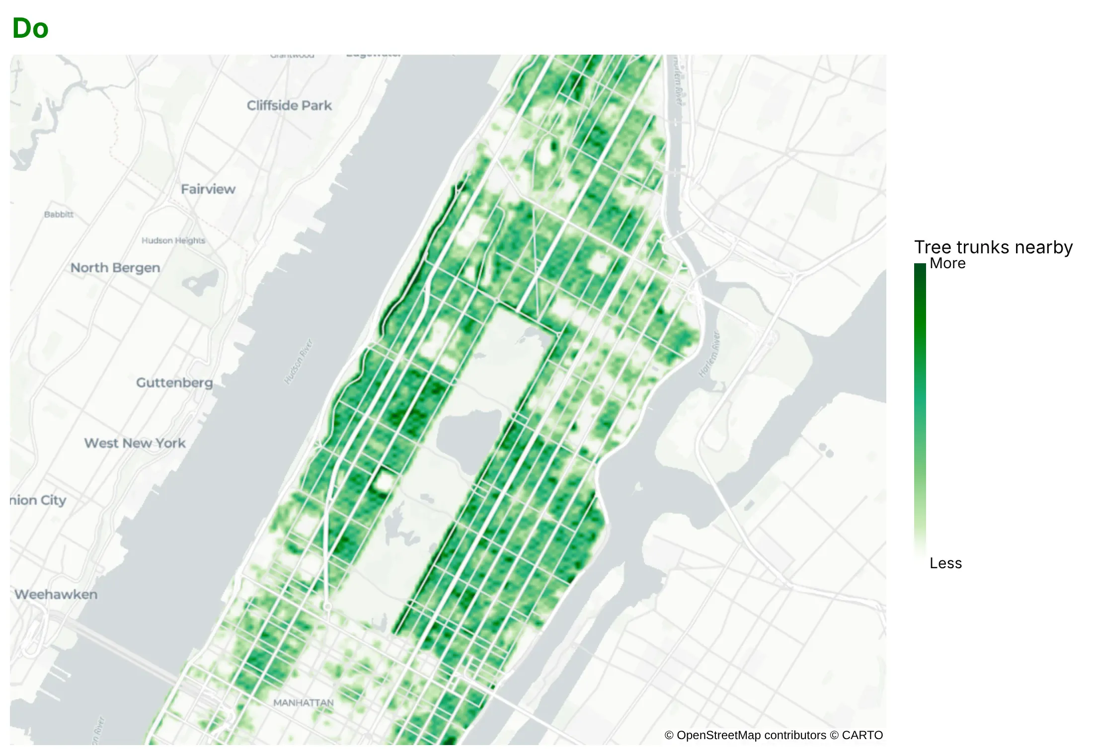
City assets. Manhattan has 62,427 street trees, and the Upper West Side has the most (5,723), then the Upper East Side (4,540) and the West Village (3,715). Data: NYC Parks, 2015 Street Tree Census.

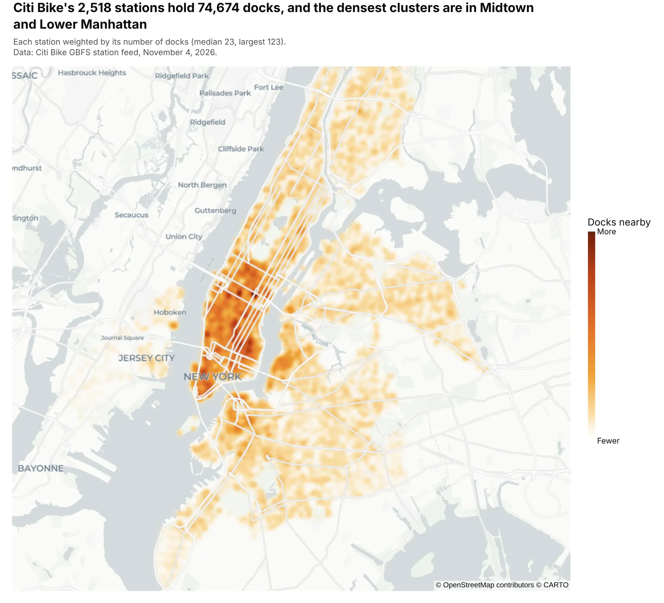
Weighting each point by a value. Citi Bike's 2,518 stations hold 74,674 docks, and weighting each station by its docks shows where the bike-share capacity is, not only where stations are. Data: Citi Bike GBFS station feed, November 4, 2026.

A short history

One of the most famous maps of where cases cluster is John Snow's. His map of the 1854 cholera outbreak in London's Soho, published in On the Mode of Communication of Cholera (1855), drew a bar for each death at its address and showed them crowded around the Broad Street pump. This is his data redrawn as a density map, from Robin Wilson's digitized version:

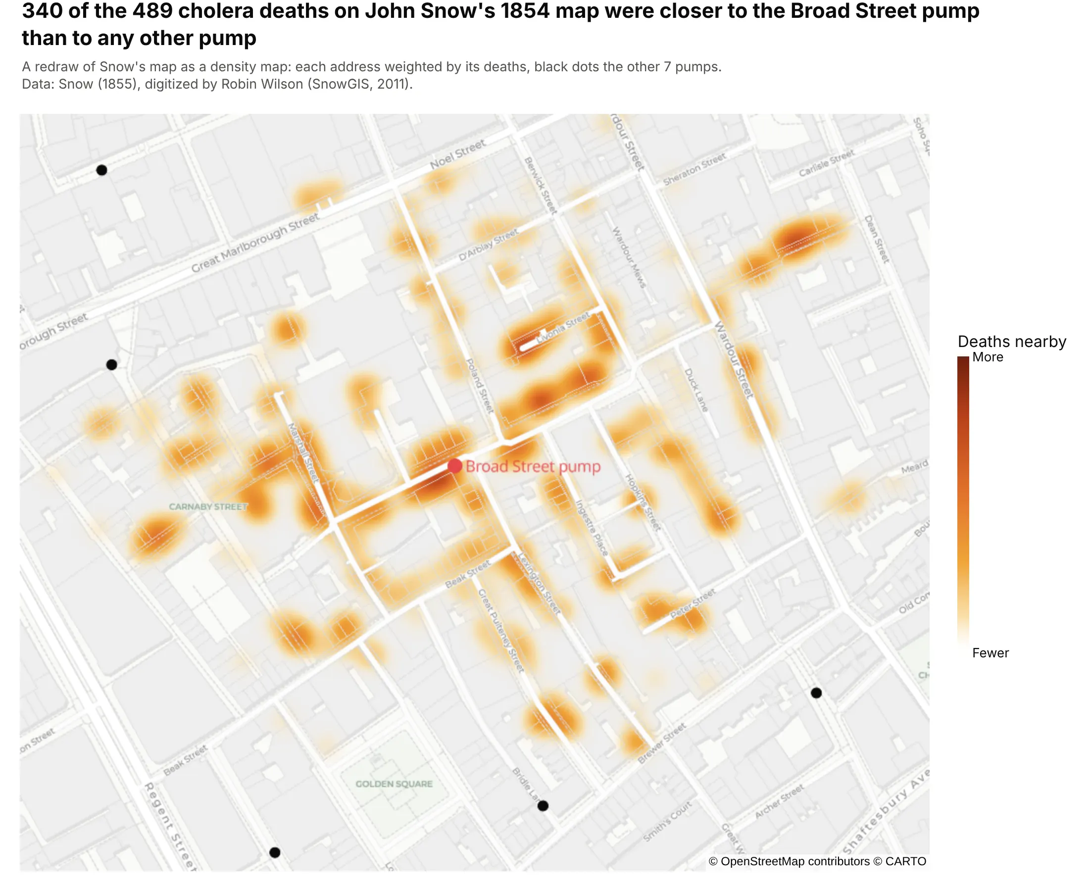
Data: Snow (1855), digitized by Robin Wilson (SnowGIS, 2011). 340 of the 489 deaths were at addresses closer to the Broad Street pump than to any other pump, in a straight line.

The smoothing behind a density map is kernel density estimation, which Rosenblatt (1956) and Parzen (1962) described for one variable, and GIS tools such as QGIS ("Heatmap (kernel density estimation)") and ArcGIS ("Kernel Density") apply to points on a map. Web maps later drew the same idea on the fly as a heat map layer. Plotly added the densitymapbox trace in plotly.js 1.49 (July 2019) and the token-free densitymap trace, drawn with MapLibre, in plotly.js 2.35 and plotly.py 5.24 (August 2024).

Alternatives to a density map

Here's the same set of 9,499 Oklahoma earthquakes drawn six ways. Some are better for the question, some worse, some just different:

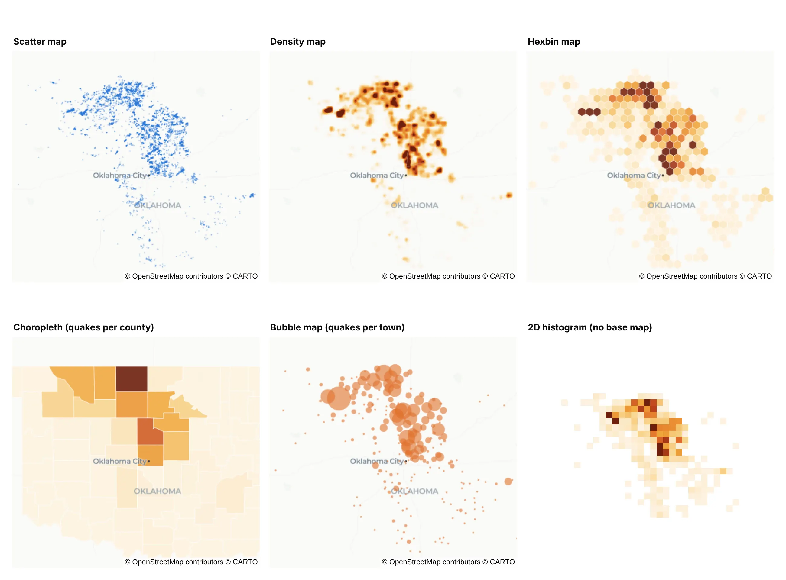
• Scatter map (better below a few thousand points). Every quake is visible and you can hover each one, but where thousands overlap, the dots merge and you can't tell 50 from 500.
• Hexbin map (better for counts you can read). Each hexagon holds an exact count, so the color bar has real numbers, though the hexagon size changes the picture the same way the radius does.
• Choropleth map (better for rates by area). Counting quakes per county gives a number per area that you can join to other county data, but Grant County looks uniformly dark even though its quakes cluster in a few spots.
• Bubble map (works too, with named places). One circle per town, sized by its quakes, reads well and labels well, but the circles overlap where towns are close together.
• 2D histogram (different). Square bins of longitude and latitude, the chart in the density plot guide and the heatmap guide, give exact counts but lose the base map, so you can't see where a cluster is.

How to make a density map

With AI

ChatGPT, Claude Code, GitHub Copilot, Cursor and other AI tools are excellent at writing Plotly code. Name Plotly in the prompt, and say what radius and weight you want, because the defaults rarely suit a large dataset:

With Plotly Studio

Plotly Studio is a desktop app where you point an AI at a dataset and it builds charts and a Dash app around your questions. Ask for a density map the same way:

Show a density map of New York's street trees from the 2015 census, with a slider for the radius, a dropdown to pick the borough and species, and the neighborhoods with the most trees listed beside the map.

Make a density map in Python or JavaScript

This is the code AI tools write under the hood. In Python, px.density_map makes the chart in one line of code, and the Plotly density heatmap documentation covers the options:

px.density_map returns a figure with one densitymap trace on a map subplot. To weight points by a value, pass that column as z and set range_color to start at 0; the next sections explain why.

In JavaScript, plotly.js draws the same trace. This example loads 2025's earthquakes straight from the USGS catalog:

Share it

Every Plotly chart has a Share chart button (the cloud icon in its toolbar) that uploads it to Plotly Cloud and gives you a link. Only you can see it until you change its visibility.

For a live app, put the chart in a Dash app and publish it with the Plotly Cloud CLI. Coding agents can run these commands for you:

If your data has to stay in your own cloud or data center, publish to Dash Enterprise instead.

Dos and don'ts

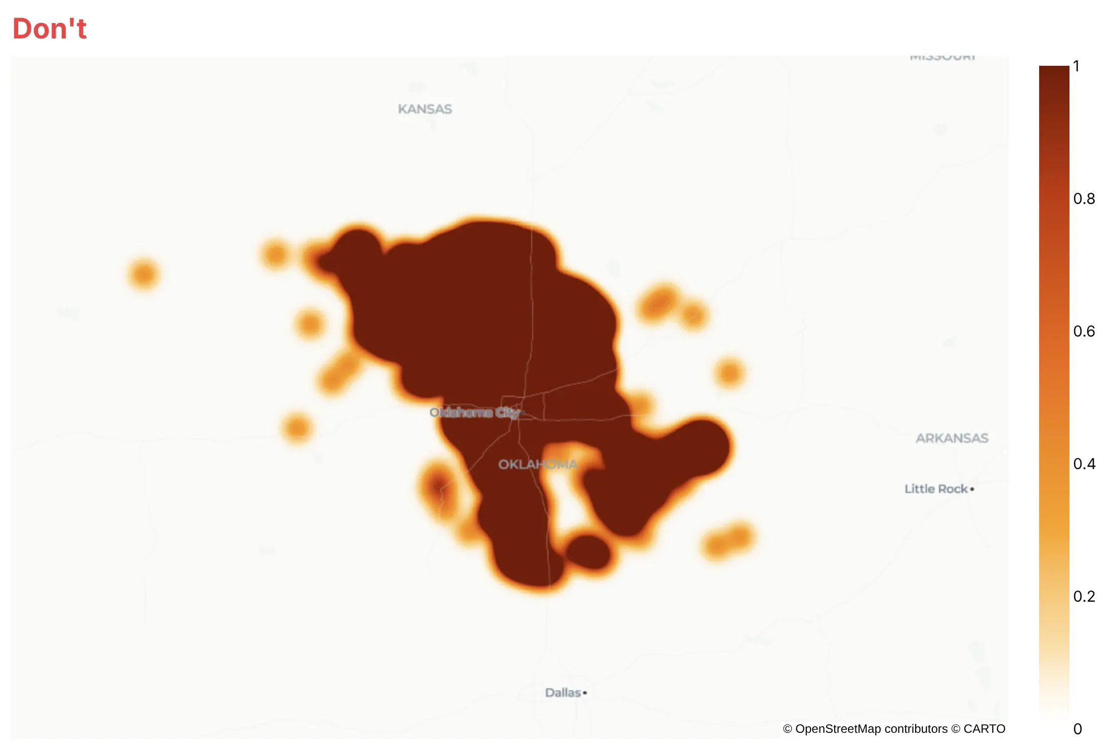
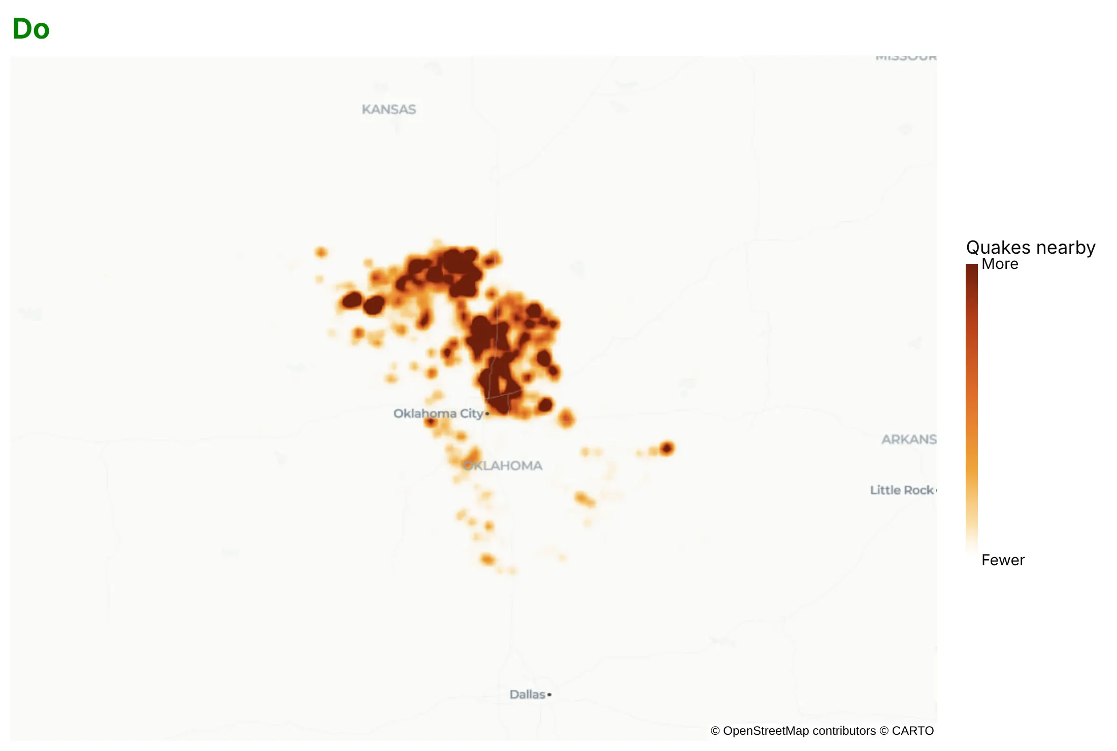
Most of the work in a density map is choosing how much each point counts and how far it spreads. Here are the 9,499 Oklahoma quakes both ways, with the same colors and base map.

Don't keep the default 30-pixel radius and full weight per point for thousands of points, which saturates every cluster into one dark mass, or leave a color bar from 0 to 1 that looks like a unit but isn't one:

Do shrink the radius until clusters separate, lower each point's weight with z and range_color so the busiest areas still differ, and label the color bar with words:

Choose the radius

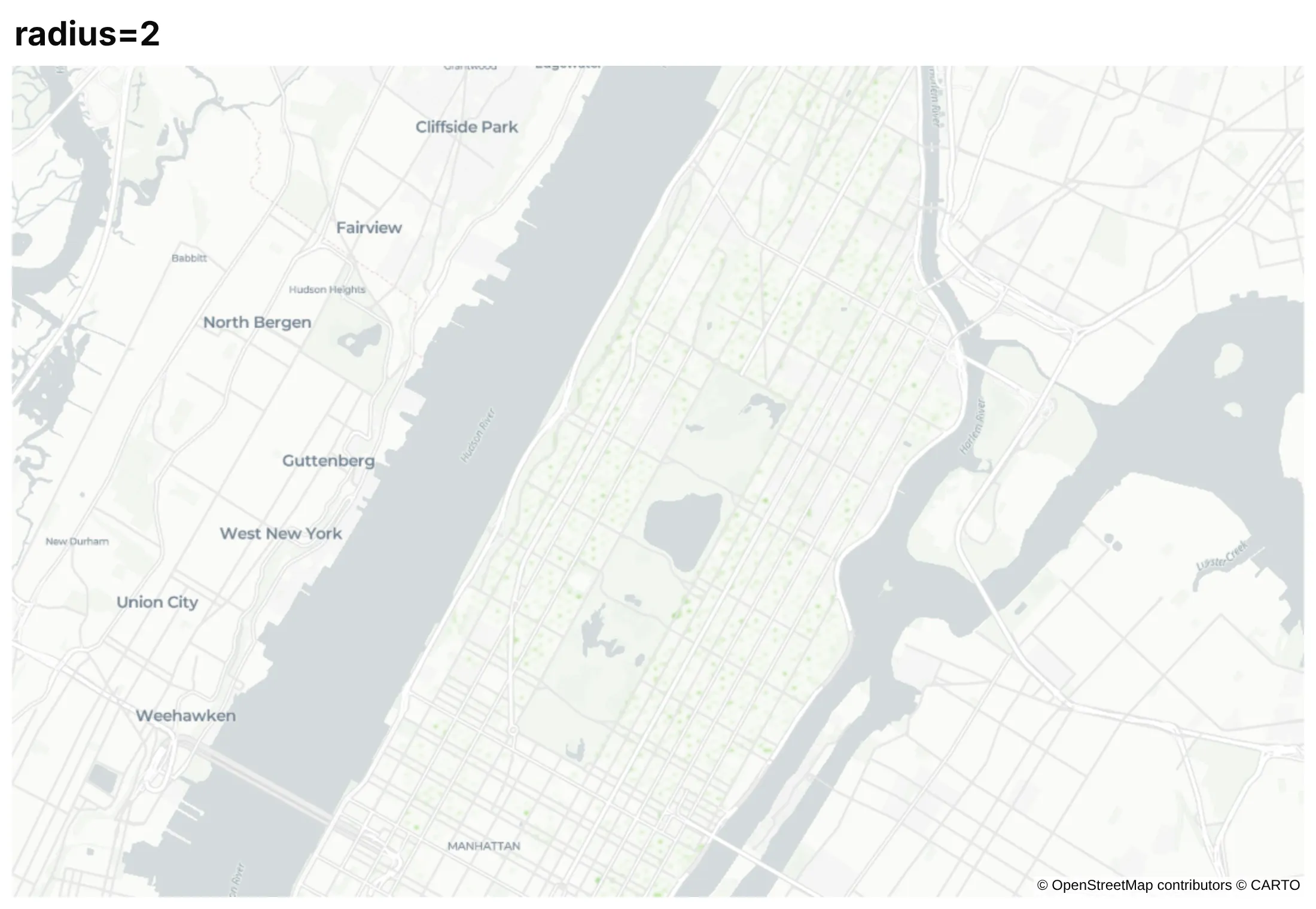
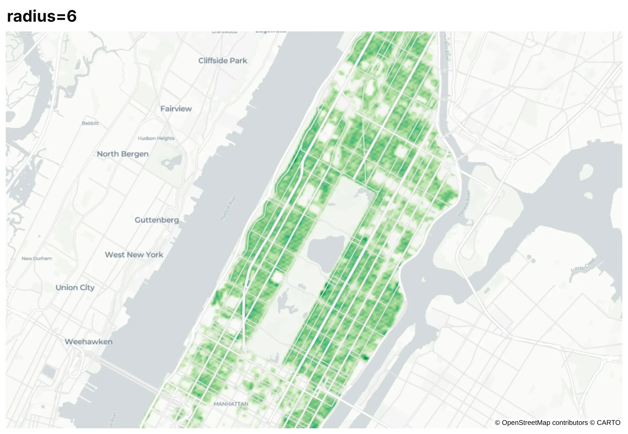
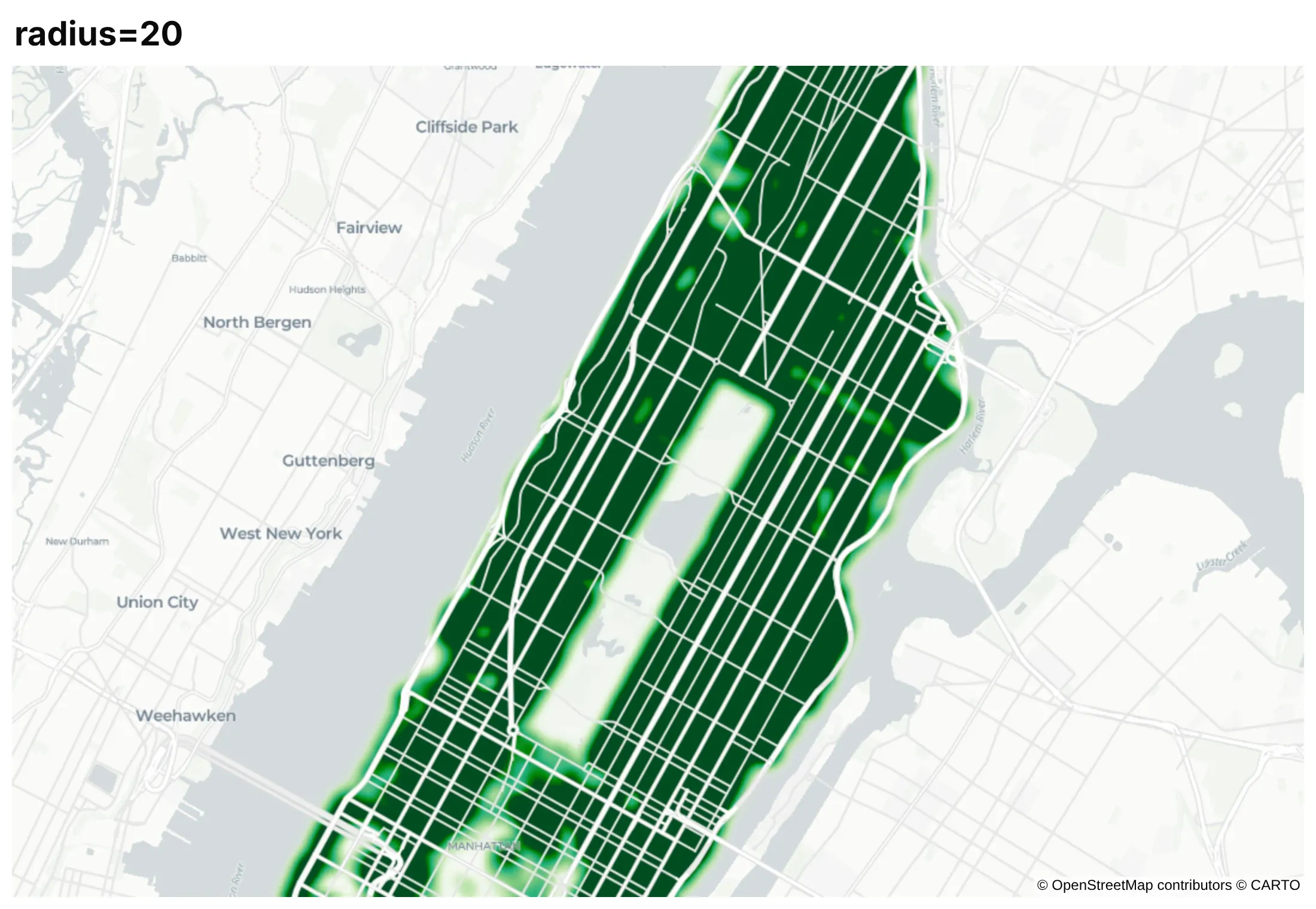
The radius is in screen pixels, so it decides how far each point spreads and how much neighboring points overlap. It changes the picture more than any other option, and it changes again when you zoom, because the same 10 pixels cover less ground at a higher zoom. Here are Manhattan's street trees with the same weight and three radii.

radius=2. Each tree is a faint dot, so you see the street grid but no pattern.

radius=6. Neighboring trees overlap enough to show which blocks and neighborhoods have the most.

radius=20. The blobs merge and saturate, and the map says only that most streets have trees.

There is no correct radius, so try a few, pick the one that matches the scale of the question (blocks, neighborhoods, regions), and say what you used in the subtitle. If readers will zoom, test the map at the zoom levels they'll use.

Set the weight range yourself

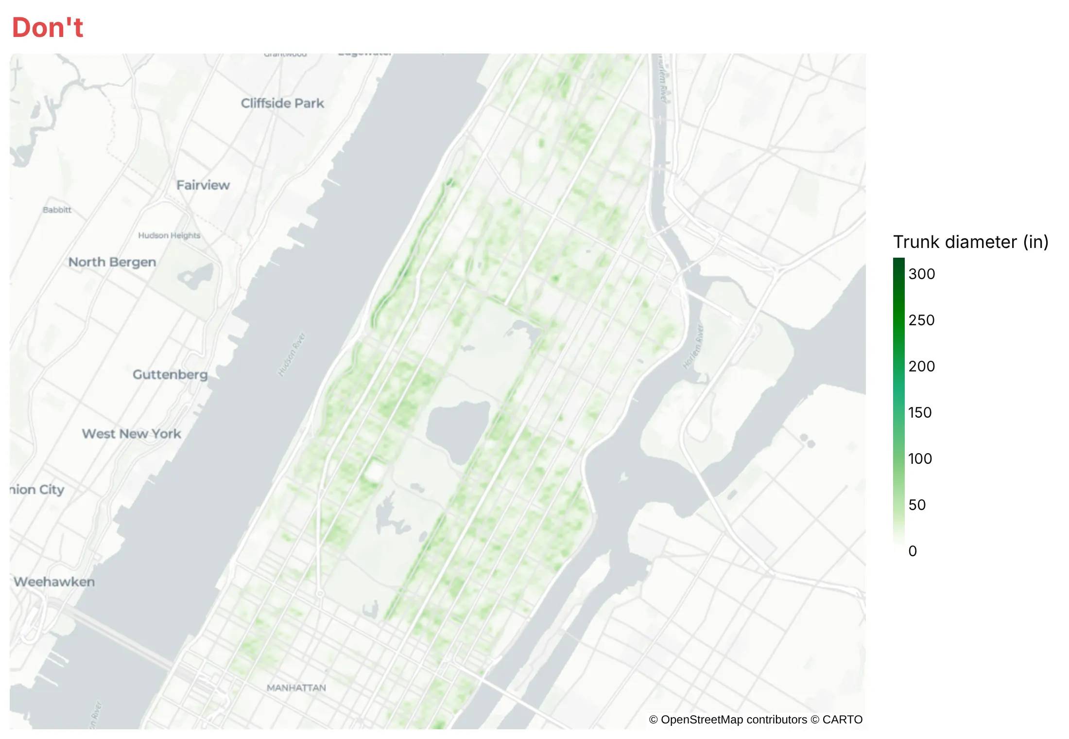
When you pass z, plotly.js scales each point's weight from the low end of the color range to the high end, so a point at the low end adds nothing and a point at the high end adds the full color. Left alone, the range runs from the smallest to the largest weight in the data. Here are Manhattan's street trees weighted by trunk diameter.

Don't leave the range to the data. Trunks run from 0 to 318 inches, so the median tree, 8 inches across, adds only a fortieth of the full color and the map looks washed out:

Do set range_color=[0, N] (or zmin=0 and zmax=N on the trace), with N the weight at which one point should reach full color. Here N is 60 inches, so the median tree adds 8/60 and the 8 trunks over 60 inches count as 60:

Checklist

Do

• Pick the radius for the scale of the question, and say what it is.
• Lower each point's weight with z and range_color when you have thousands of points, so dense areas don't all saturate.
• Start range_color at 0 whenever you pass z.
• Label the color bar with words such as Fewer and More, because the density has no unit.
• Use a light, label-light base map (carto-positron) for warm colors and a dark one for fire or light data.
• Mark the few points the story needs (the largest quake, the pump) with a scatter_map trace on top.
• Write a title that states the takeaway and a subtitle with the source and period.

Don't

• Read the color as a count or a rate; it's a relative density.
• Compare two density maps with different radii, weights or zooms.
• Weight by a value with a long tail (deposits, revenue) without checking that a few points don't drown out the rest; a bubble map often works better.
• Use a density map for rates per person or per area; a choropleth does that honestly.

Options to customize

A density map in Plotly is px.density_map or a go.Densitymap trace on a map subplot, so these are the options that matter most. The full lists are in the px.density_map reference and the densitymap trace reference.

1. lat, lon: the point locations, in degrees.
2. radius: how far each point spreads, in screen pixels (default 30); also takes one value per point.
3. z: a weight per point; a weight of 10 counts like 10 points in the same spot.
4. range_color (zmin, zmax on the trace): the weights that map to no color and full color; start it at 0.
5. color_continuous_scale: the colors; the first one is made transparent so the base map shows through.
6. opacity: the opacity of the whole density layer.
7. map_style: the base map, such as carto-positron, carto-darkmatter, open-street-map or white-bg; none needs a token.
8. center, zoom: the starting view; plotly.js 4 fits the view to the data when you leave them out.
9. hover_name, hover_data: what shows when you hover a point.
10. animation_frame: one frame per year or month, with a slider.
11. below (go.Densitymap): which base map layer to draw under; "" puts the density on top of labels.
12. fig.add_scattermap(...): points, labels and markers on top of the density.

More density map examples

Six more density maps built from real public data, each with its source, the technique that makes it work and a prompt to rebuild it.

1. Where America's bank branches are

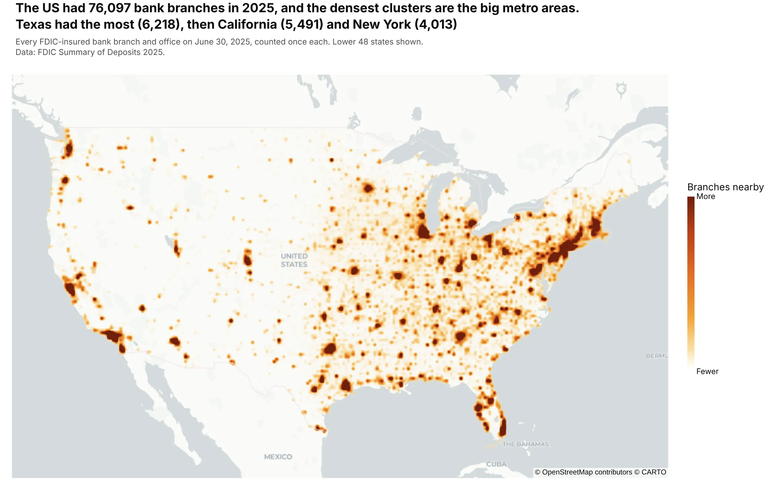
The US had 76,097 bank branches and offices on June 30, 2025, and the densest clusters are the big metro areas. Texas had the most branches (6,218), then California (5,491) and New York (4,013). Data: FDIC Summary of Deposits 2025.

Tip: weight every branch the same when the question is where people can reach a bank.

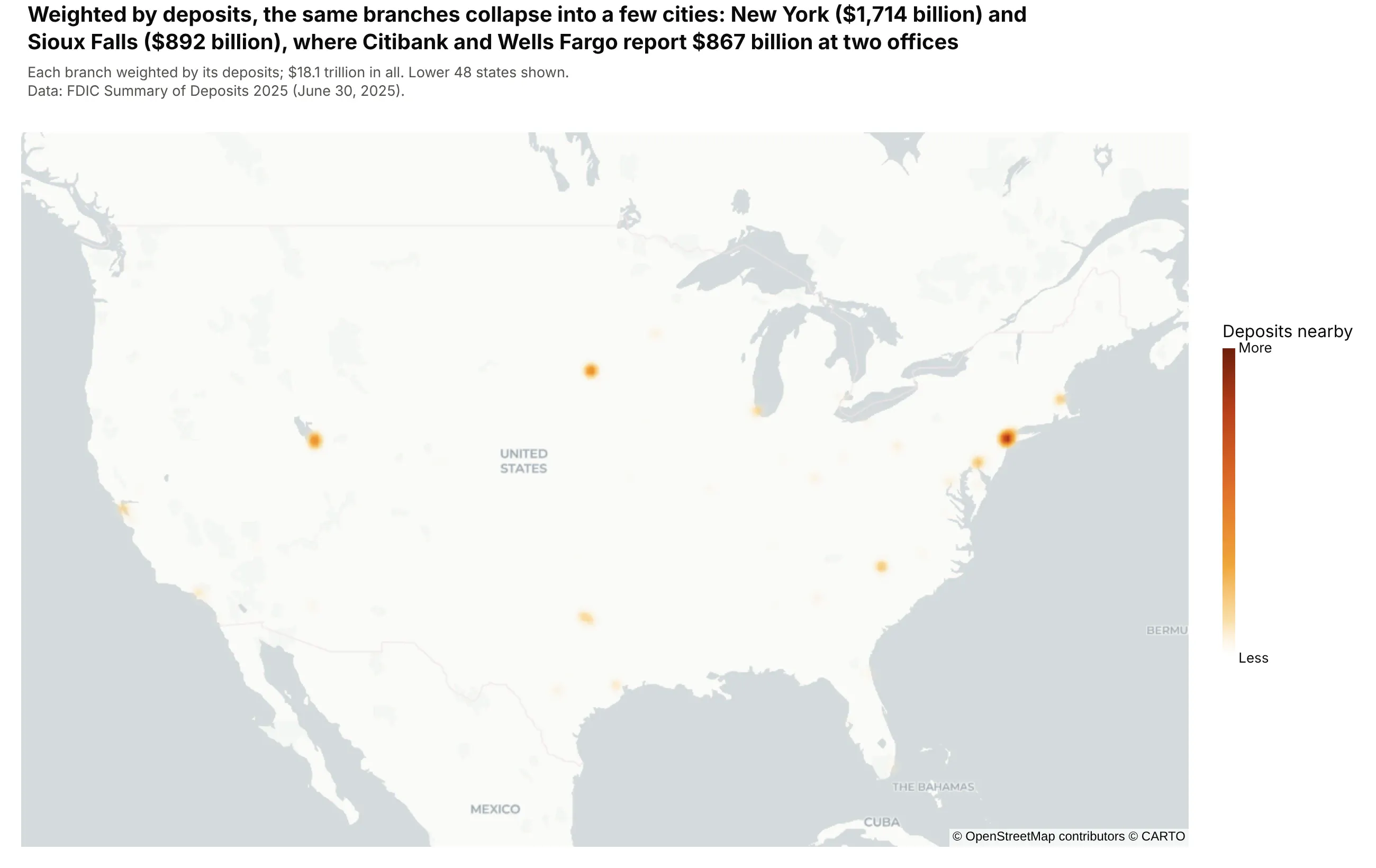
Another way to see it: weighting each branch by its deposits collapses the map into a few cities, because banks book deposits at a few offices: Citibank and Wells Fargo report $867 billion at two offices in Sioux Falls. For a heavy-tailed value like this, a bubble map of the top cities is clearer.

2. Where Phase 3 trials recruit

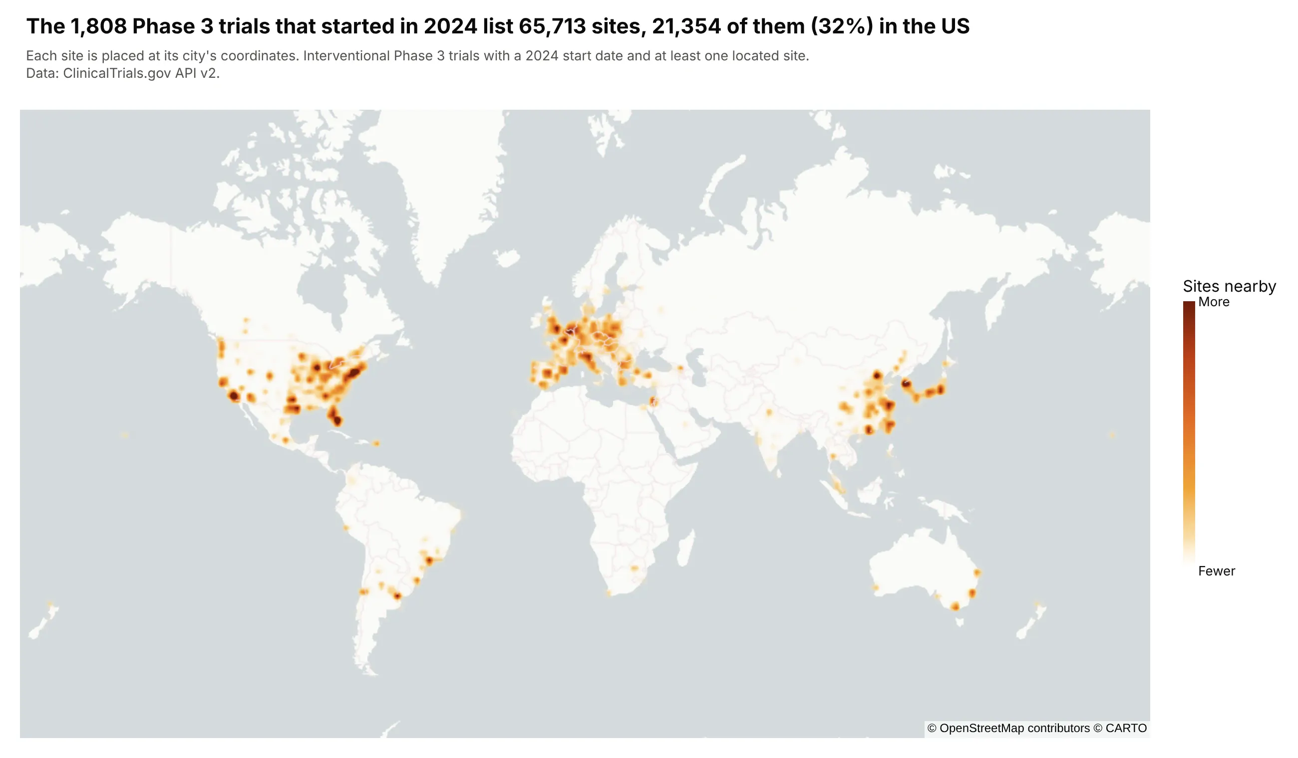
The 1,808 Phase 3 trials that started in 2024 list 65,713 sites, and 21,354 of them (32%) are in the US. Seoul has the most sites of any city, 749. Data: ClinicalTrials.gov API v2.

Tip: when many points share the same coordinates, as sites in one city do here, a density map adds them up where a scatter map draws one dot.

3. A week of fire seen from space

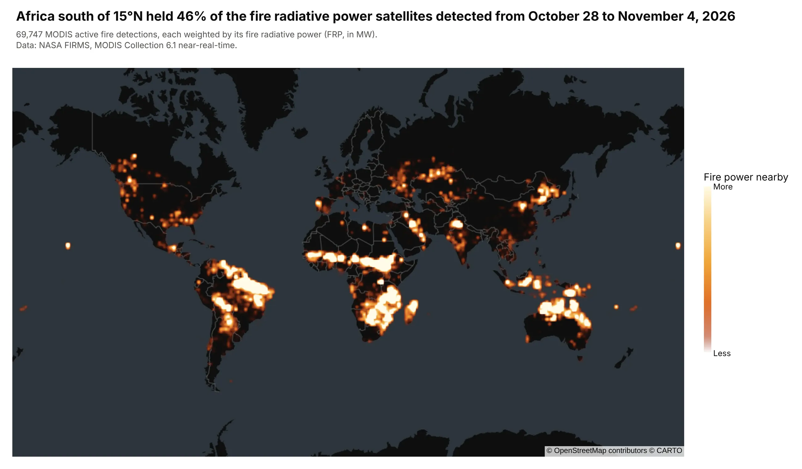
Africa south of 15°N held 46% of the fire radiative power that NASA's MODIS satellites detected from October 28 to November 4, 2026. Weighting each of the 69,747 detections by its power shows where the most energy was released. Data: NASA FIRMS, MODIS Collection 6.1.

Tip: for fire or light data, use the carto-darkmatter base map and a scale that ends in white.

4. 75 years of US tornadoes

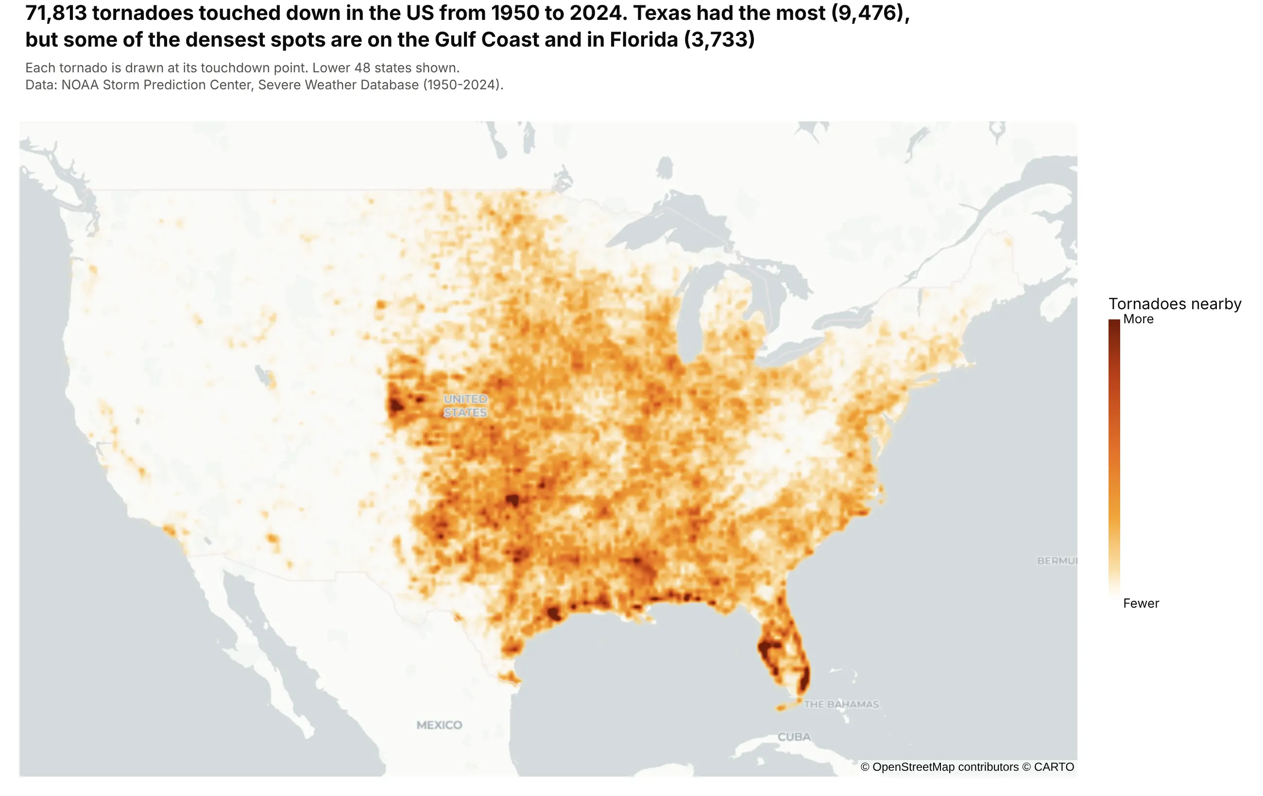
71,813 tornadoes touched down in the US from 1950 to 2024. Texas had the most (9,476), but some of the densest spots are on the Gulf Coast and in Florida (3,733). Data: NOAA Storm Prediction Center, Severe Weather Database.

Tip: a density map counts events, so filter to strong tornadoes (mag >= 3) if the question is about damage rather than frequency.

5. Oklahoma's orphan wells

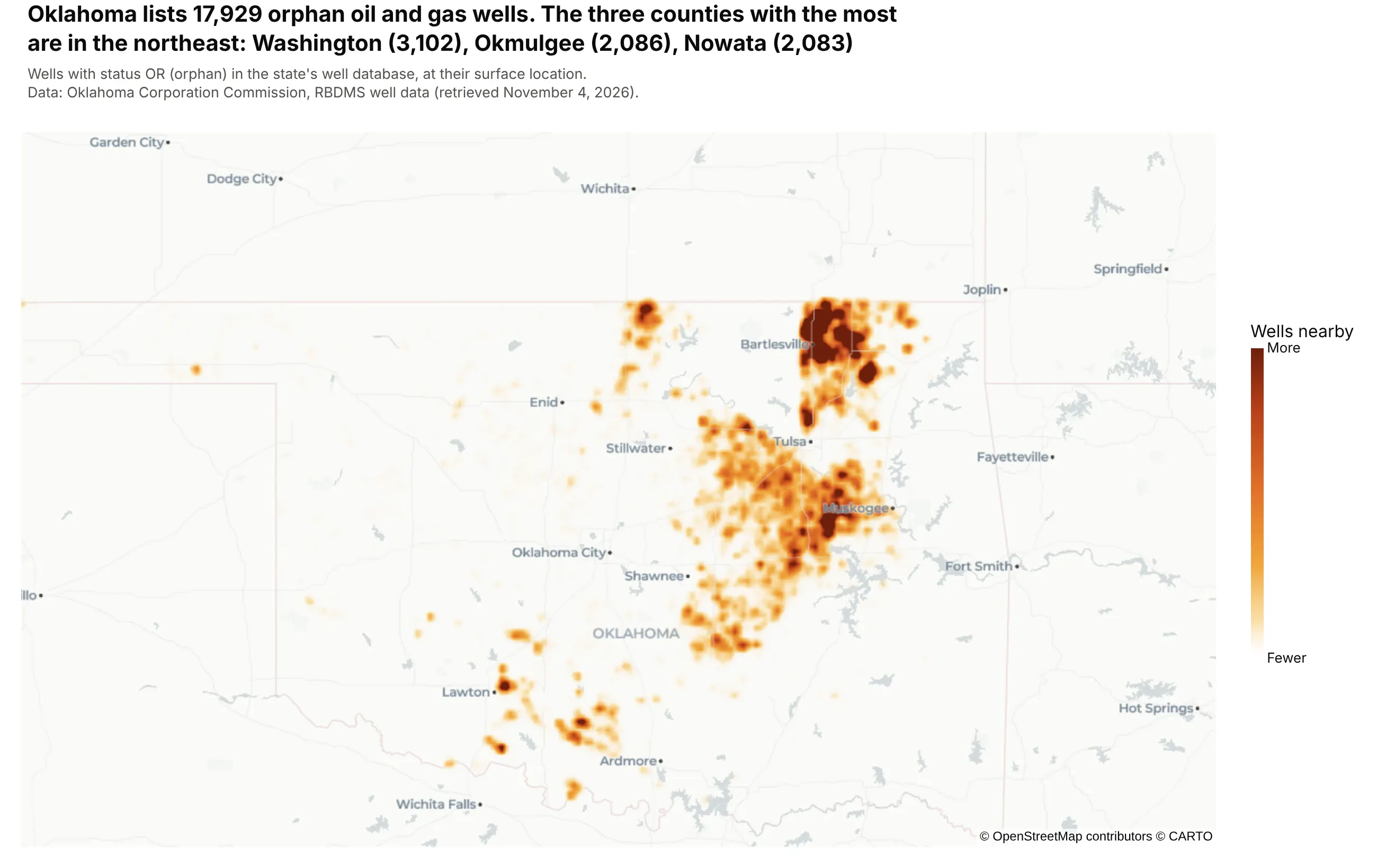
Oklahoma lists 17,929 orphan oil and gas wells, wells with no responsible operator. The three counties with the most are in the northeast: Washington (3,102), Okmulgee (2,086) and Nowata (2,083). Data: Oklahoma Corporation Commission, RBDMS well data.

Tip: wells a few hundred meters apart merge into dots at state zoom, so a 7-pixel radius shows which fields hold the most.

6. The rise and fall of Oklahoma's earthquakes

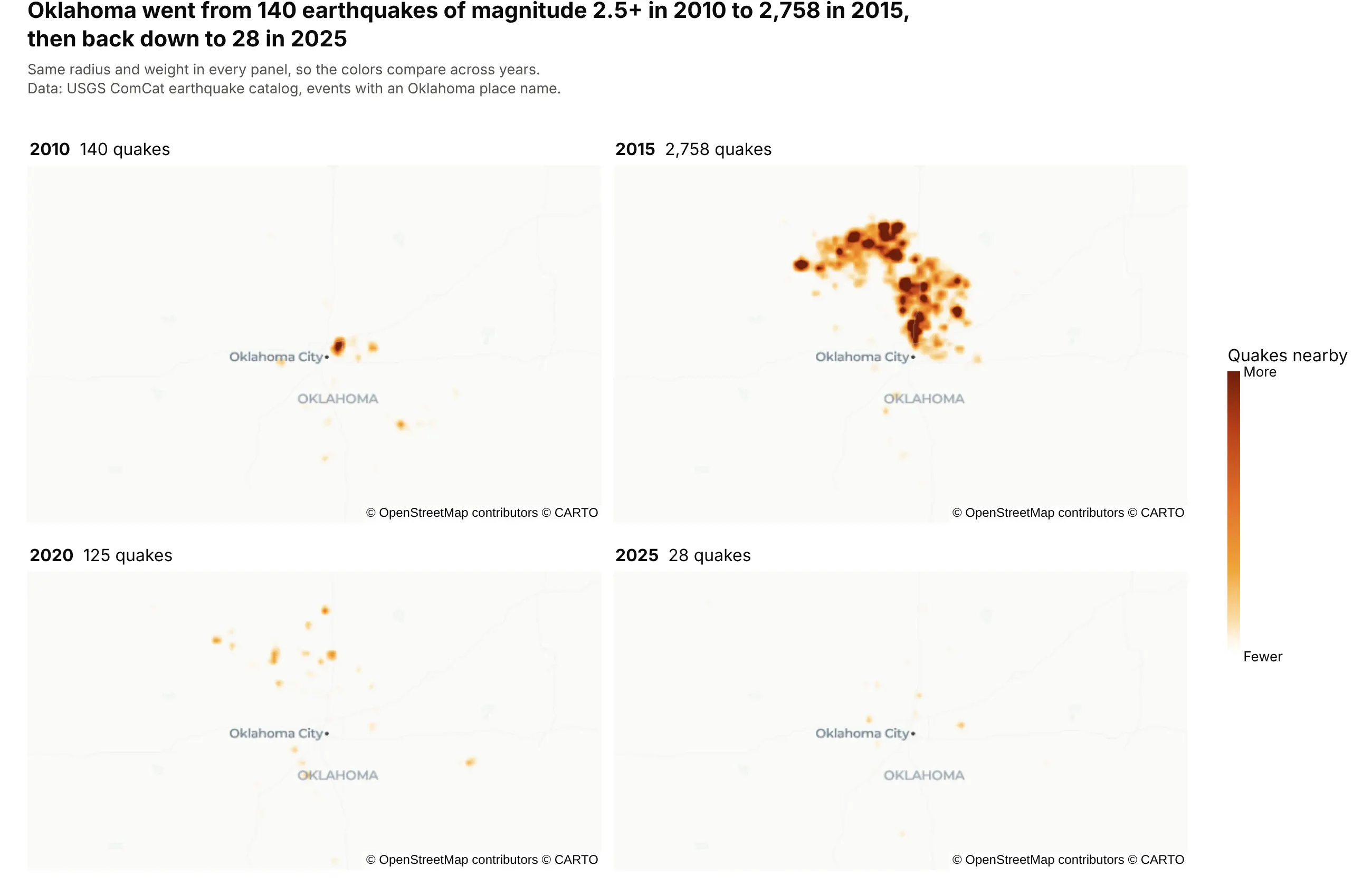
Oklahoma went from 140 earthquakes of magnitude 2.5 or more in 2010 to 2,758 in 2015, then back down to 28 in 2025. Splitting the main example by year shows the boom and the decline that a single map hides. Data: USGS ComCat earthquake catalog.

Tip: use the same radius, weight and color range in every panel so the years compare; in an interactive chart, animation_frame="year" does the same with a slider.