Bubble Maps - A Complete Guide

TL;DR

• A bubble map puts a circle on a map at each place, and the circle's area shows an amount there: the capacity of a power plant, the people in a city, the passengers at an airport.
• Bubble maps are also known as proportional symbol maps, scaled symbol maps and, when the sizes come in classes, graduated symbol maps, and are similar to bubble charts, choropleth maps and density maps.
• Use one for counts and totals. A choropleth colors whole regions, so big, empty regions look important; a bubble shows the amount without the region's size getting in the way.
• You can make a bubble map with Plotly in one line of code with px.scatter_geo (an outline map) or px.scatter_map (a street tile map). Size the bubbles by area, which Plotly Express does by default.

What is a bubble map?

Bubble maps look like this:

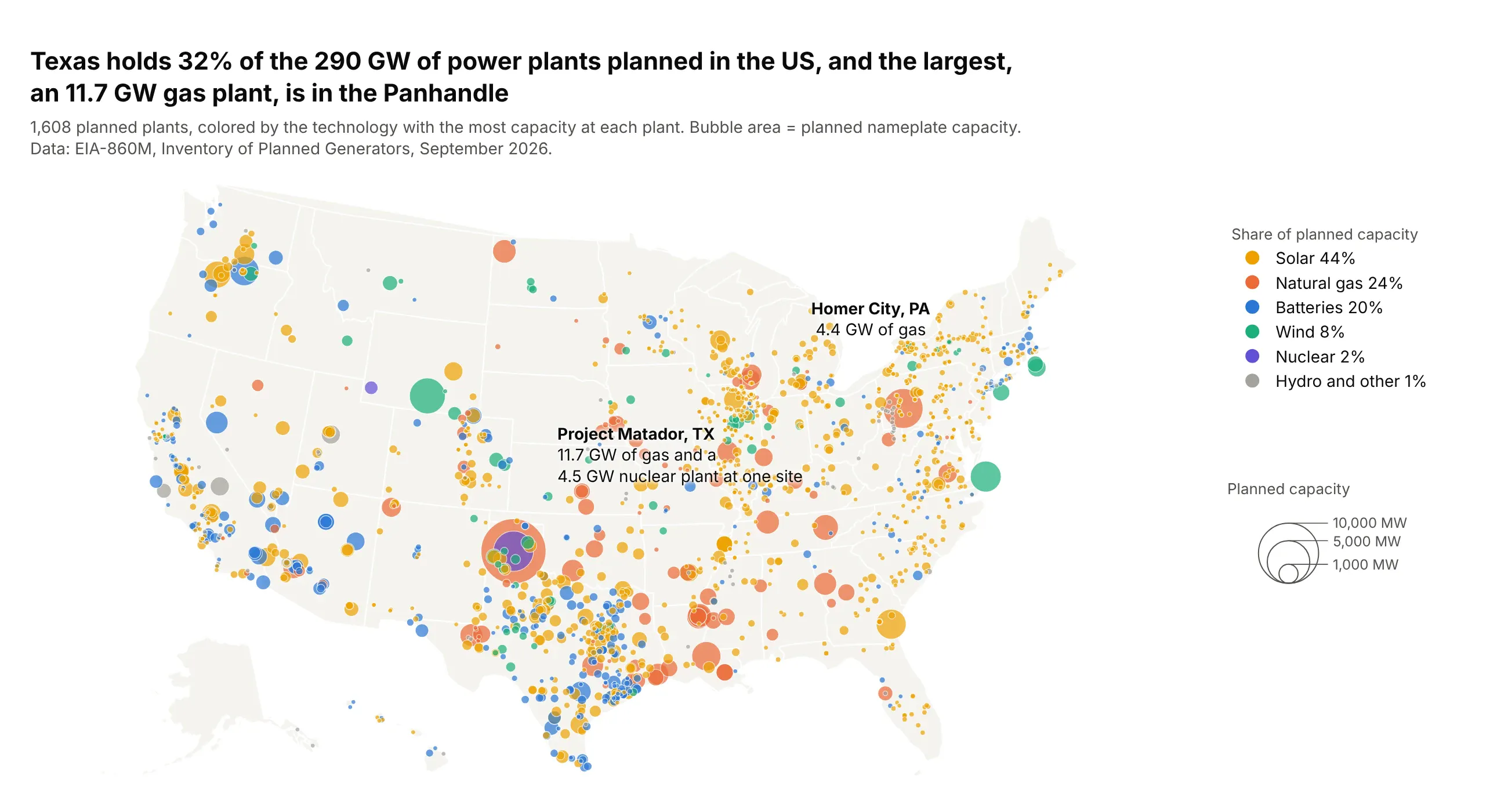
Data: EIA-860M, Inventory of Planned Generators, September 2026.

How do you read a bubble map? In the example above, notice these things:

• Each bubble is one planned power plant, drawn at its latitude and longitude, so the clusters are real places: the solar and battery projects around Houston and Dallas, the gas plants along the Gulf Coast.
• The area of a bubble is the plant's planned capacity. The 10,000 MW circle in the legend has 10 times the area of the 1,000 MW circle, but only about 3.2 times its width, so compare areas, not widths.
• Color is the technology with the most capacity at the plant. Solar has 1,023 of the 1,608 plants but 44% of the capacity, because the average solar plant is 124 MW and the average gas plant 690 MW.
• The biggest bubble, Project Matador in the Texas Panhandle, is 11.7 GW of gas with a 4.5 GW nuclear plant drawn inside it at the same site. Texas holds 32% of the 290 GW planned in the US.

It's often used for charts like these:

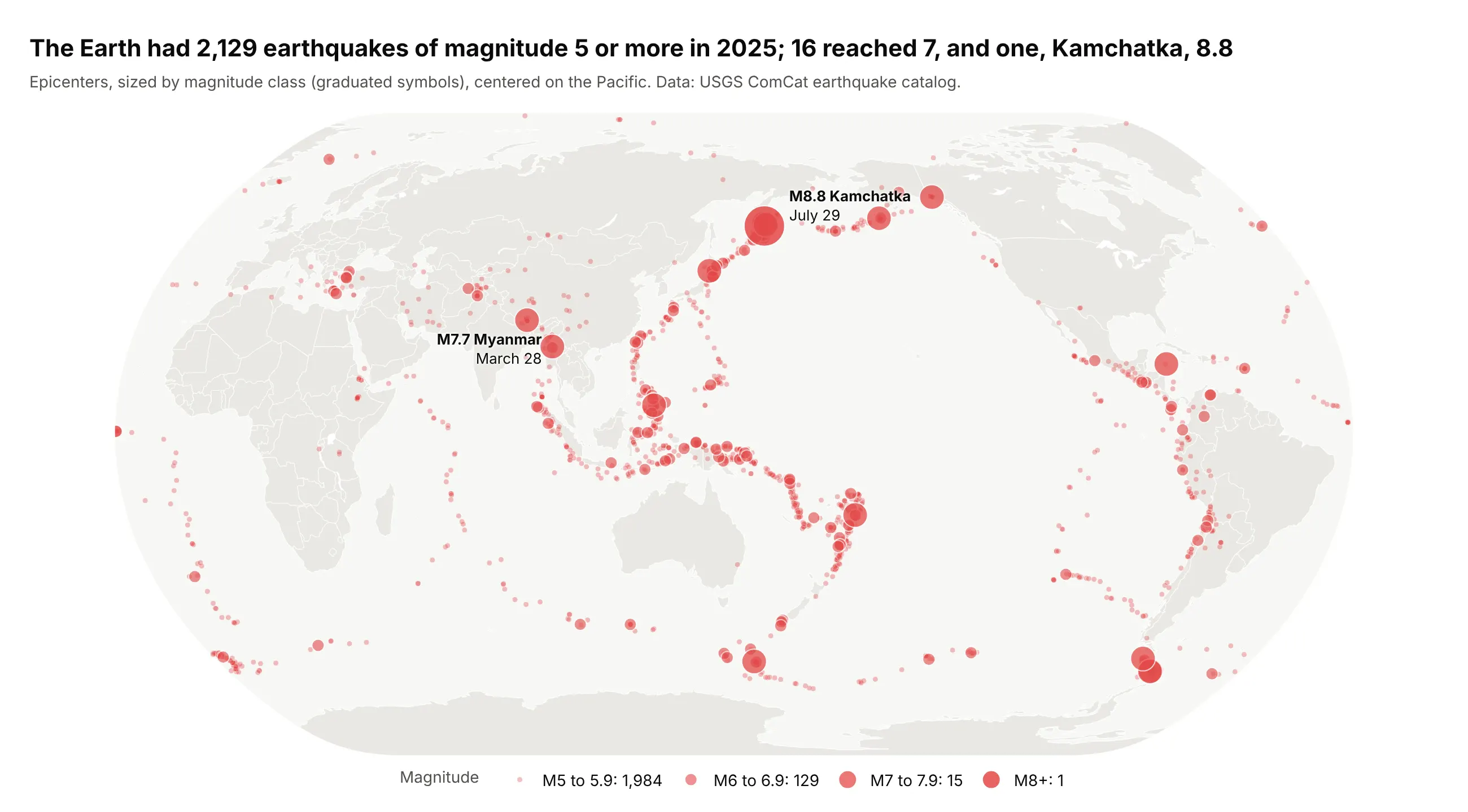
Earthquakes. The classic bubble map in seismology: 2,129 earthquakes of magnitude 5 or more in 2025, 16 of them 7 or more, drawn as graduated symbols because magnitude is a logarithmic scale. Data: USGS ComCat earthquake catalog.

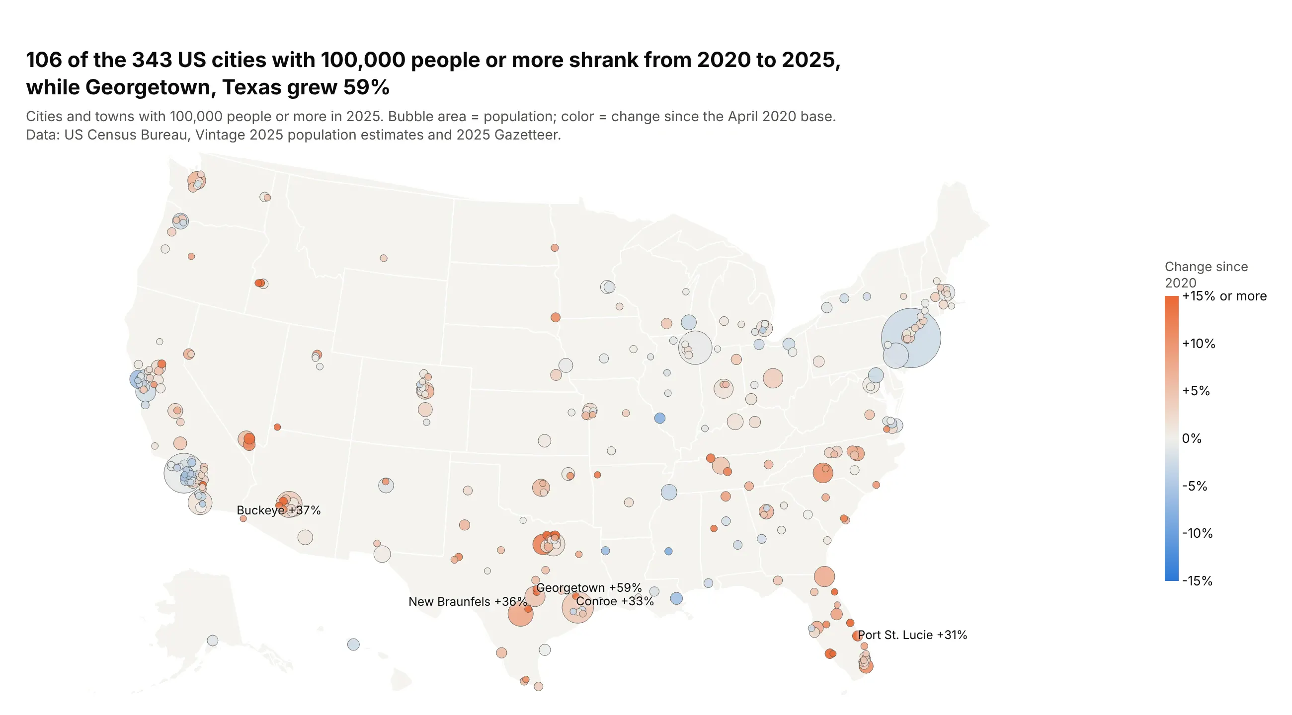
City populations. The oldest use of the chart: 106 of the 343 US cities with 100,000 people or more shrank from 2020 to 2025, while Georgetown, Texas grew 59%. Data: US Census Bureau, Vintage 2025 population estimates.

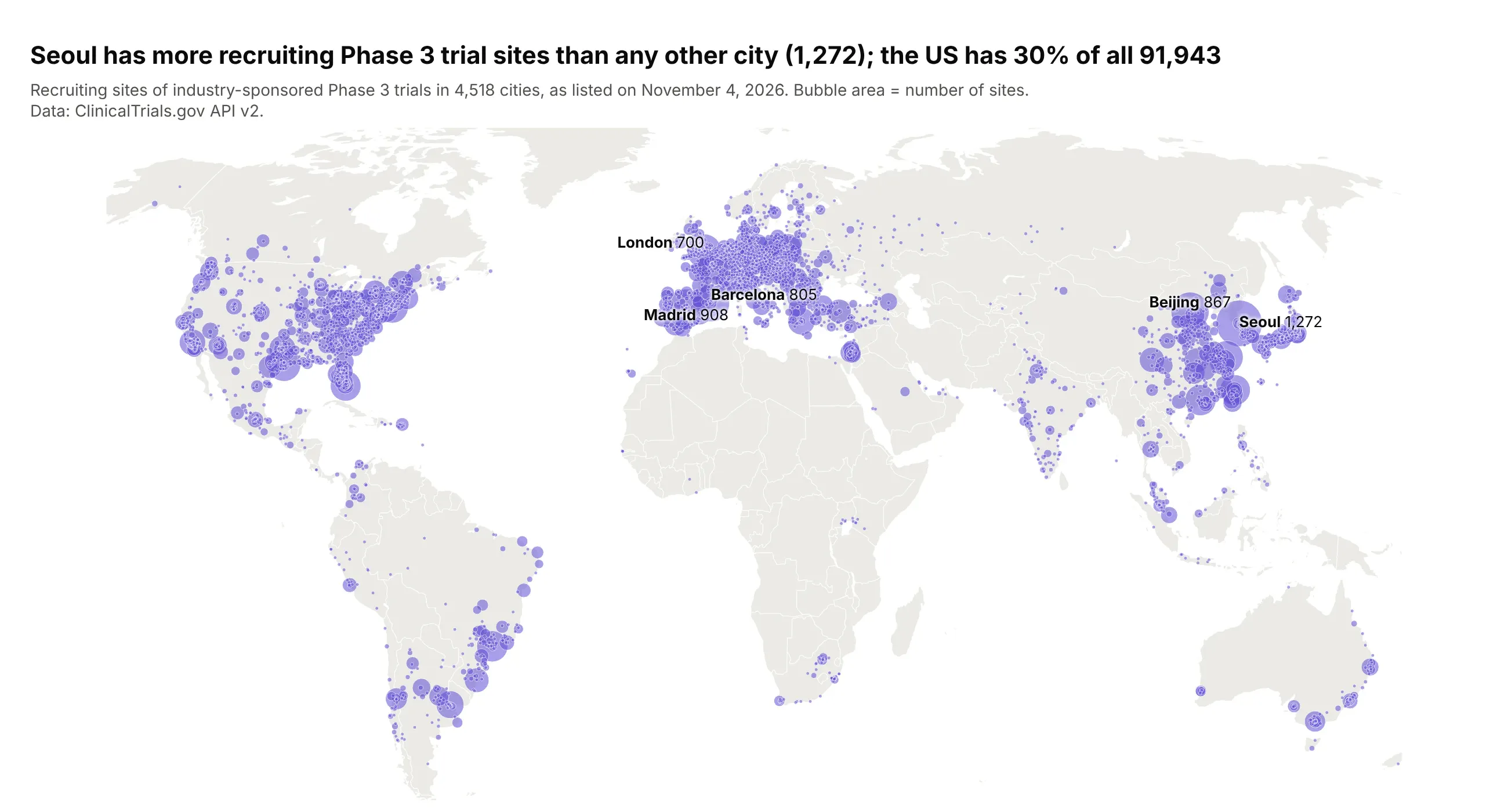
Sites and facilities. Seoul has 1,272 recruiting sites for industry-sponsored Phase 3 trials, more than any other city, and the US has 30% of all 91,943. Data: ClinicalTrials.gov API v2.

A short history

Bubbles on maps came before bubble charts. The geographer Arthur Robinson traced the first map that sized point symbols in proportion to a number to the 1837 maps drawn for the Irish Railway Commissioners, whose circles showed city populations (Robinson 1955). Charles Joseph Minard drew proportional circles for regions in the 1850s, including an 1858 map of the meat sent to Paris from each French department, with pie charts inside the circles (Wikipedia, proportional symbol map). In the 1950s and 1970s James Flannery tested how people read them and found that readers underestimate the larger of two circles (Flannery 1971), which is why a size legend matters.

Alternatives to a bubble map

Here's the same planned power plant data drawn six ways. Some are better for the question, some worse, some just different:

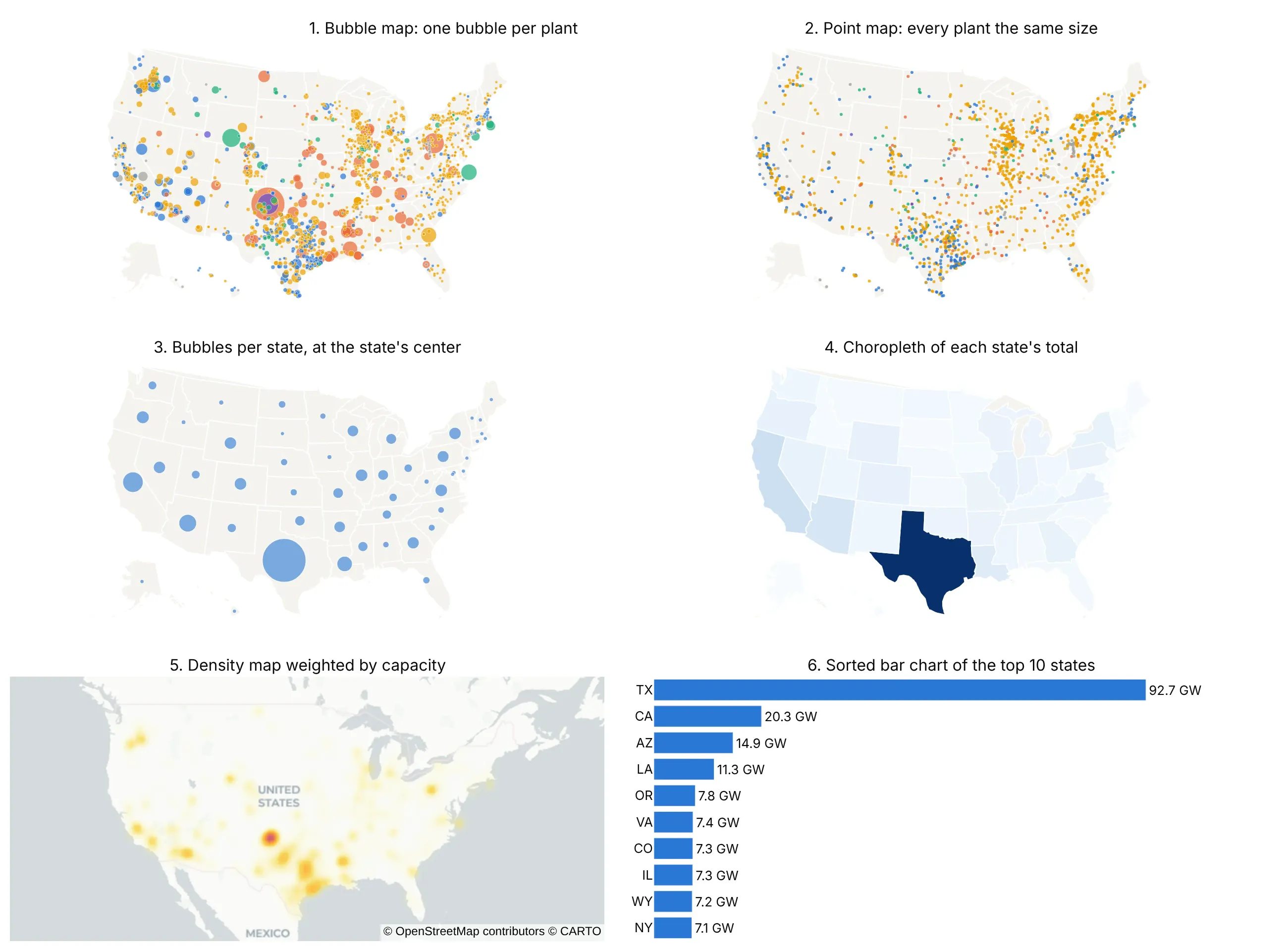
• Point map, or dot map (different). Every plant is the same size, so it shows where projects are and how many, and solar's 1,023 plants take over. It answers "how many" but not "how much"; a dot density map, where each dot stands for a fixed amount, is the same idea for regions.
• Bubbles per state (works too, for regions). When your numbers are totals by region, one bubble per state or country at its center keeps the advantage over a choropleth. Plotly places them from state or country codes, as in example 1 below.
• Choropleth map (worse for counts). Coloring each state by its total makes Texas the only dark state and paints large, empty states by area. Choropleths are the better chart for rates and shares, such as capacity per person.
• Density map (different). A smoothed heat map weighted by capacity shows hot spots, here the Texas Panhandle and Houston, and handles tens of thousands of points, but you can't read a single plant.
• Sorted bar chart (better for ranking). Texas at 92.7 GW is more than four times California at 20.3 GW, which is easier to read from bars than from circles. You lose the map.
• Bubble chart (different). The same circles on x and y axes instead of longitude and latitude, for comparing three numbers rather than places.

How to make a bubble map

With AI

ChatGPT, Claude Code, GitHub Copilot, Cursor and other AI tools are excellent at writing Plotly code. Name Plotly in the prompt, and say how the bubbles should be sized and drawn:

With Plotly Studio

Plotly Studio is a desktop app where you point an AI at a dataset and it builds charts and a Dash app around your questions. Ask for a bubble map the same way:

Show a bubble map of every recruiting Phase 3 trial site by city, sized by the number of sites, with the city, country and number of trials on hover and a filter by sponsor type.

Make a bubble map in Python or JavaScript

This is the code AI tools write under the hood. In Python, px.scatter_geo makes the chart in one line of code, and the Plotly bubble map documentation covers more options:

Plotly Express sets sizemode="area" and computes one sizeref for every color, so bubbles compare across traces and size_max is the width in pixels of the biggest one. With go.Scattergeo you set them yourself: the default sizemode is "diameter", and sizeref = 2 * max(values) / size_max**2 with sizemode="area" gives the same result. To draw the bubbles on a street map instead, swap px.scatter_geo for px.scatter_map, as in the Manhattan example below. px.scatter_mapbox was deprecated in plotly 6.0 and removed in plotly 7.0, and px.scatter_map takes the same arguments without a Mapbox token (migration guide).

In JavaScript, plotly.js draws the same thing from a scattergeo trace:

Share it

Every Plotly chart has a Share chart button (the cloud icon in its toolbar) that uploads it to Plotly Cloud and gives you a link. Only you can see it until you change its visibility.

For a live app, put the chart in a Dash app and publish it with the Plotly Cloud CLI. Coding agents can run these commands for you:

If your data has to stay in your own cloud or data center, publish to Dash Enterprise instead.

Dos and don'ts

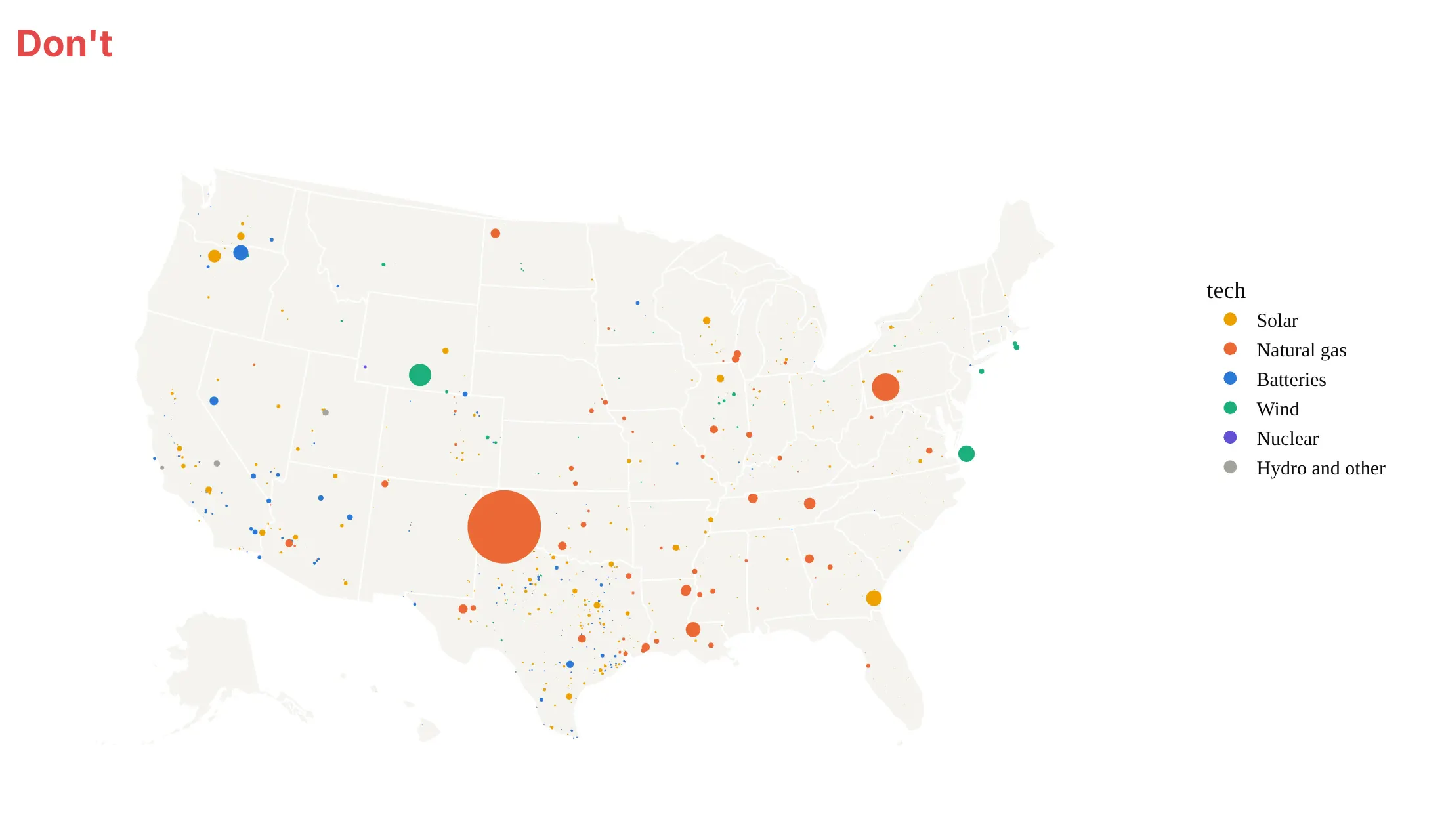
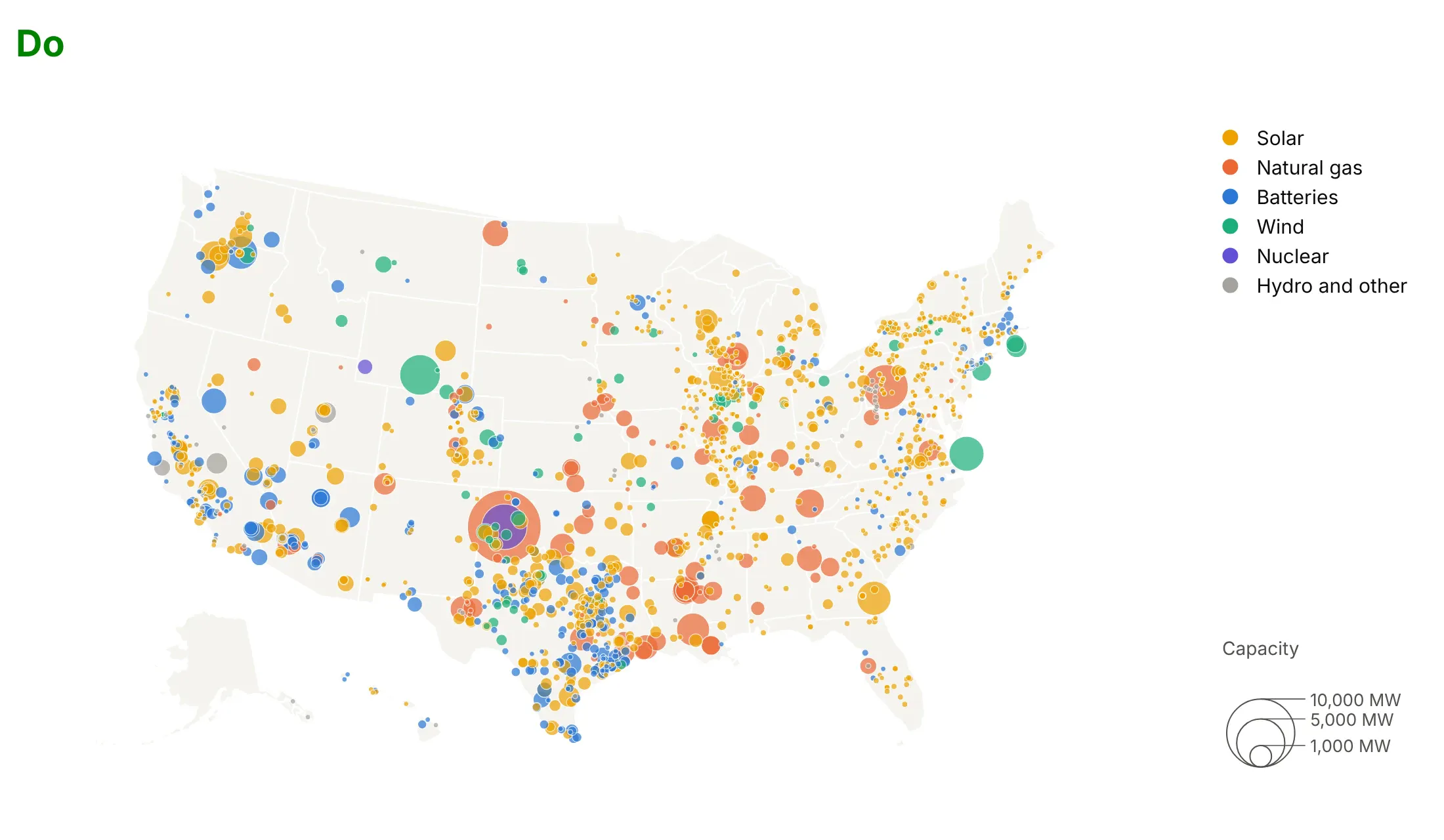
Most of what makes a bubble map honest is how the bubbles are sized and drawn. Here are the planned power plants both ways, in the same colors.

Don't size the bubbles by diameter (go.Scattergeo's default), which makes a plant with twice the capacity look four times as big and shrinks a 1,000 MW plant to a 5-pixel dot, draw the small plants first so big bubbles cover them, use opaque bubbles with no outline, leave out the size legend, or keep a default serif font and a raw column name as the legend title:

Do size by area, draw the big plants first so small ones sit on top, use partly transparent bubbles with a thin white outline so overlaps stay readable, and add a size legend:

Choose proportional or graduated symbols

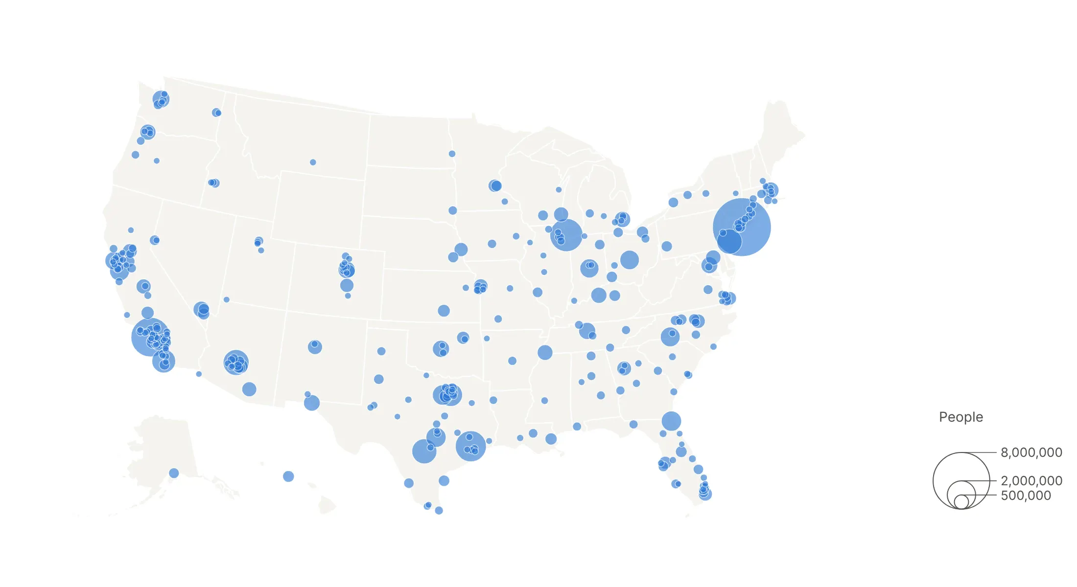
Proportional symbols. Each bubble's area is exactly proportional to the value, so New York's 8.6 million people get a bubble 34 times the area of a city of 250,000. Use it when the reader should compare amounts.

Graduated symbols. Values are grouped into classes and each class gets one size, like a choropleth's color classes. Use it when the range is too wide for proportional bubbles, or when the values are on a logarithmic scale like earthquake magnitude, and print the class ranges in the legend.

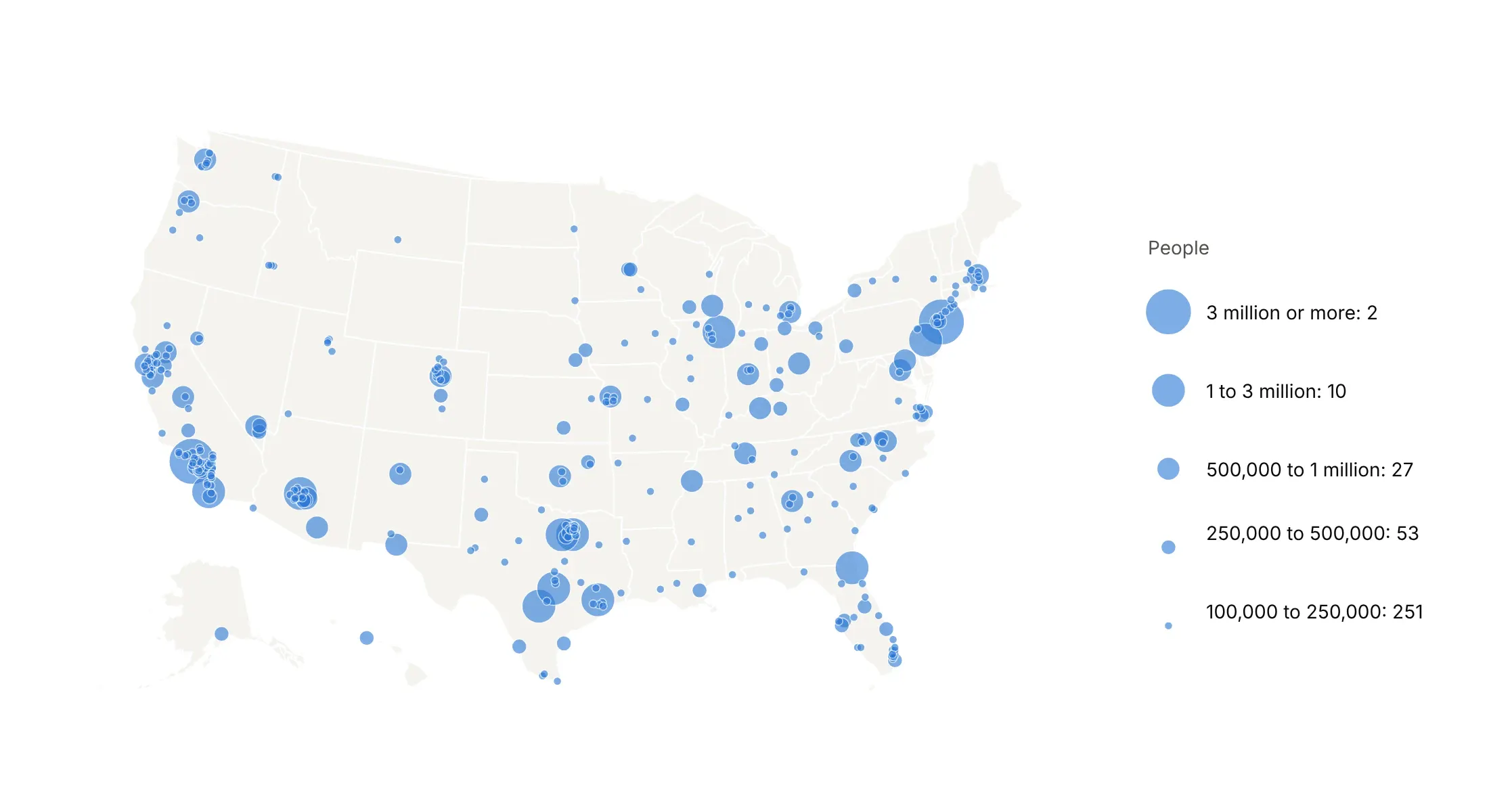
Handle overlapping bubbles

Some overlap is normal, and a bubble map whose bubbles never touch has them too small to compare. Draw the largest first (sort by size, descending), use opacity from 0.5 to 0.8 and a thin outline, and keep sizemin at 1 to 3 pixels so the smallest places stay visible. When one area is too crowded, zoom in on a tile map with px.scatter_map, aggregate to cities or regions, or switch to a density map.

Checklist

Do

• Size bubbles by area (sizemode="area"), with sizeref set from the largest value.
• Sort by size, descending, so small bubbles are drawn on top.
• Use partial opacity and a thin outline where bubbles overlap.
• Add a size legend with two or three round values.
• Put counts and totals on size, and rates or categories on color.
• Write a title that states the takeaway.

Don't

• Size by diameter or radius, which exaggerates the big values.
• Use a bubble map for rates and percentages; use a choropleth for those.
• Size bubbles by a negative number; size by the absolute value and color by the sign, as in example 6.
• Read a bubble at a region's center as a point location; say in the subtitle when bubbles stand for regions.

Options to customize

A bubble map in Plotly is a scattergeo trace (px.scatter_geo) on an outline map or a scattermap trace (px.scatter_map) on a tile map, so these are the options that matter most. The full lists are in the scattergeo reference, the scattermap reference and the geo map configuration page.

1. px.scatter_geo(lat=..., lon=..., size=...): one bubble per row, at a latitude and longitude, sized by a column.
2. locations, locationmode: place bubbles by ISO-3 country code, US state code or country name instead of coordinates; Plotly puts each at the region's center.
3. size_max (Plotly Express): the width in pixels of the largest bubble.
4. marker.sizemode="area": makes area, not diameter, proportional to the value; Plotly Express sets it, go.Scattergeo defaults to "diameter".
5. marker.sizeref: the scale; 2 * max(values) / size_max**2 makes the largest bubble size_max pixels wide. Use one sizeref for every trace you want to compare.
6. marker.sizemin: the smallest bubble in pixels, so tiny values stay visible.
7. marker.opacity, marker.line: transparency and outline for overlapping bubbles.
8. color, color_continuous_scale, range_color: a category or a rate on color.
9. hover_name, hover_data, hovertemplate: the place's name and values on hover.
10. scope, projection_type, fitbounds: the outline map's region ("usa", "europe", "world"), projection ("albers usa", "natural earth", "orthographic") and zoom to the data.
11. showland, landcolor, showcountries, subunitcolor: the outline map's base layers; a light gray land color keeps the bubbles in front.
12. px.scatter_map(..., map_style=..., zoom=..., center=...): the same bubbles on a MapLibre tile map, for city scale; "carto-positron" and "open-street-map" need no token.
13. animation_frame: one frame per year or month, for bubbles that grow and shrink over time.

More bubble map examples

Six more bubble maps built from real public data, each with its source, the technique that makes it work and a prompt to rebuild it.

1. CO2 emissions by country

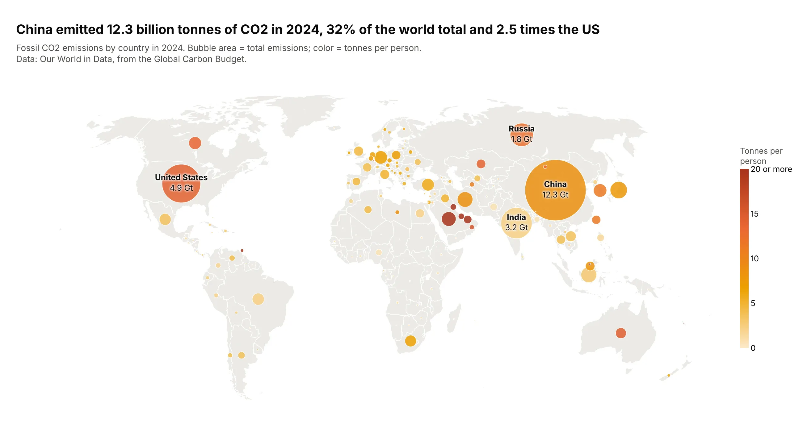
China emitted 12.3 billion tonnes of CO2 in 2024, 32% of the world total and 2.5 times the US, but the US emitted 14.2 tonnes per person against China's 8.7. Total goes on size and the per-person rate on color, so one map answers both. Data: Our World in Data, from the Global Carbon Budget.

Tip: px.scatter_geo(df, locations="iso_code", size=...) places each bubble at the country's center from its ISO-3 code, with no latitude or longitude in the data.

2. Bank deposits in Manhattan on a street map

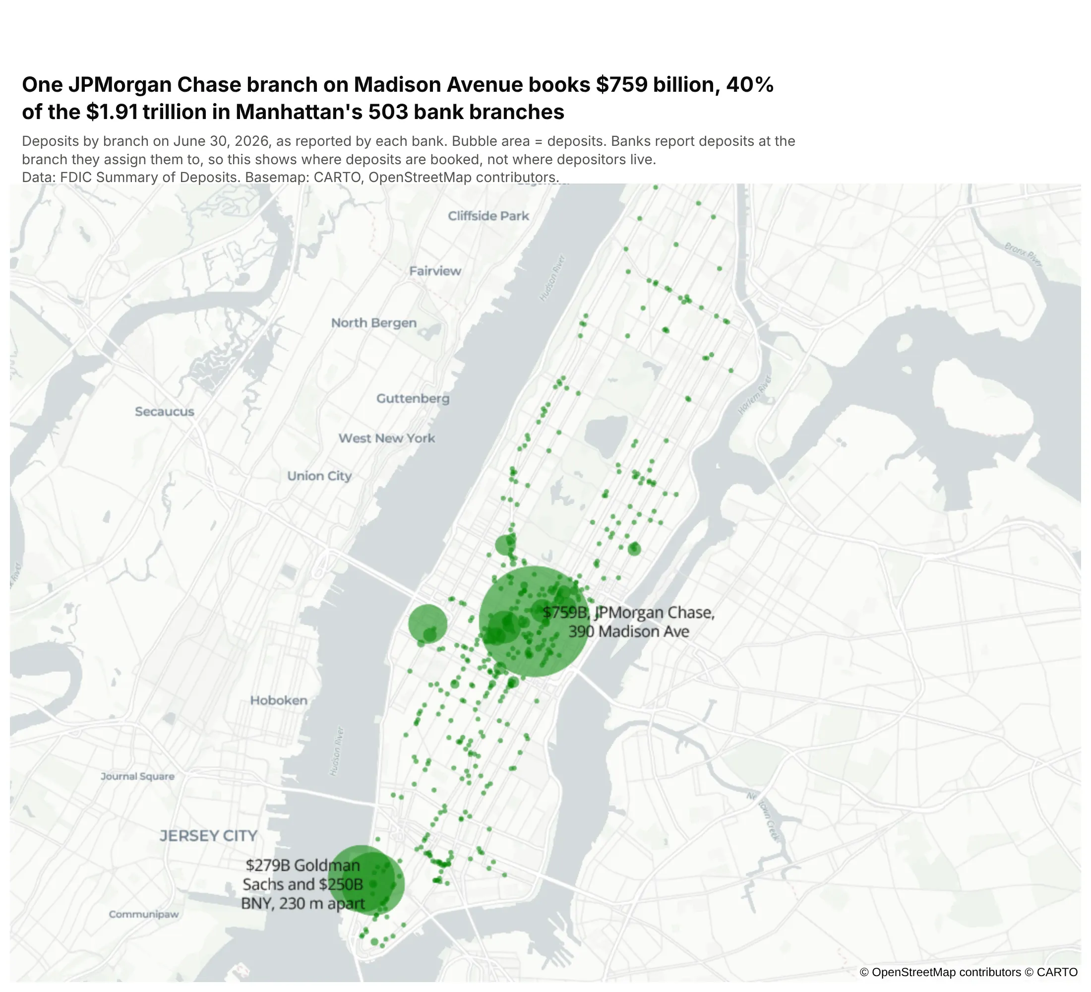
One JPMorgan Chase branch at 390 Madison Avenue books $759 billion, 40% of the $1.91 trillion in Manhattan's 503 bank branches. Banks report each deposit at the branch they assign it to, and the largest banks assign most of theirs to a few offices, so the map shows where deposits are booked, not where depositors live. Data: FDIC Summary of Deposits, June 30, 2026.

Tip: at city scale, use px.scatter_map with map_style="carto-positron" so readers can find the bubbles by street.

3. Passengers at US airports

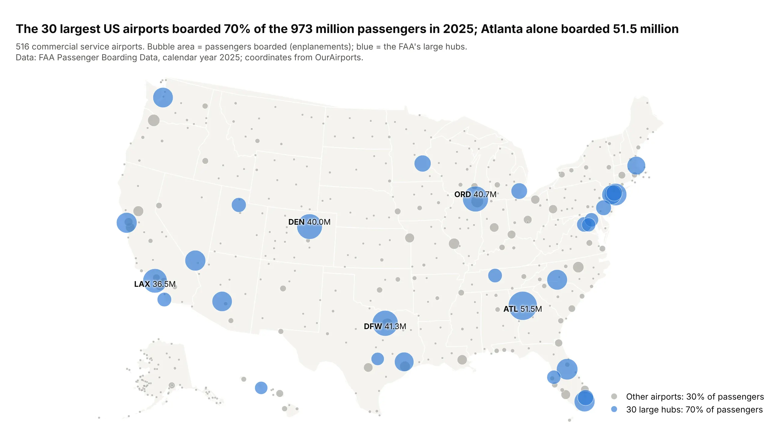
The 30 largest US airports boarded 70% of the 973 million passengers in 2025, and Atlanta alone boarded 51.5 million. The other 486 airports share the remaining 30%. Data: FAA Passenger Boarding Data, calendar year 2025; coordinates from OurAirports.

Tip: when you split bubbles into traces by category, give every trace the same sizeref so the sizes stay comparable.

4. Large wildfires of 2025

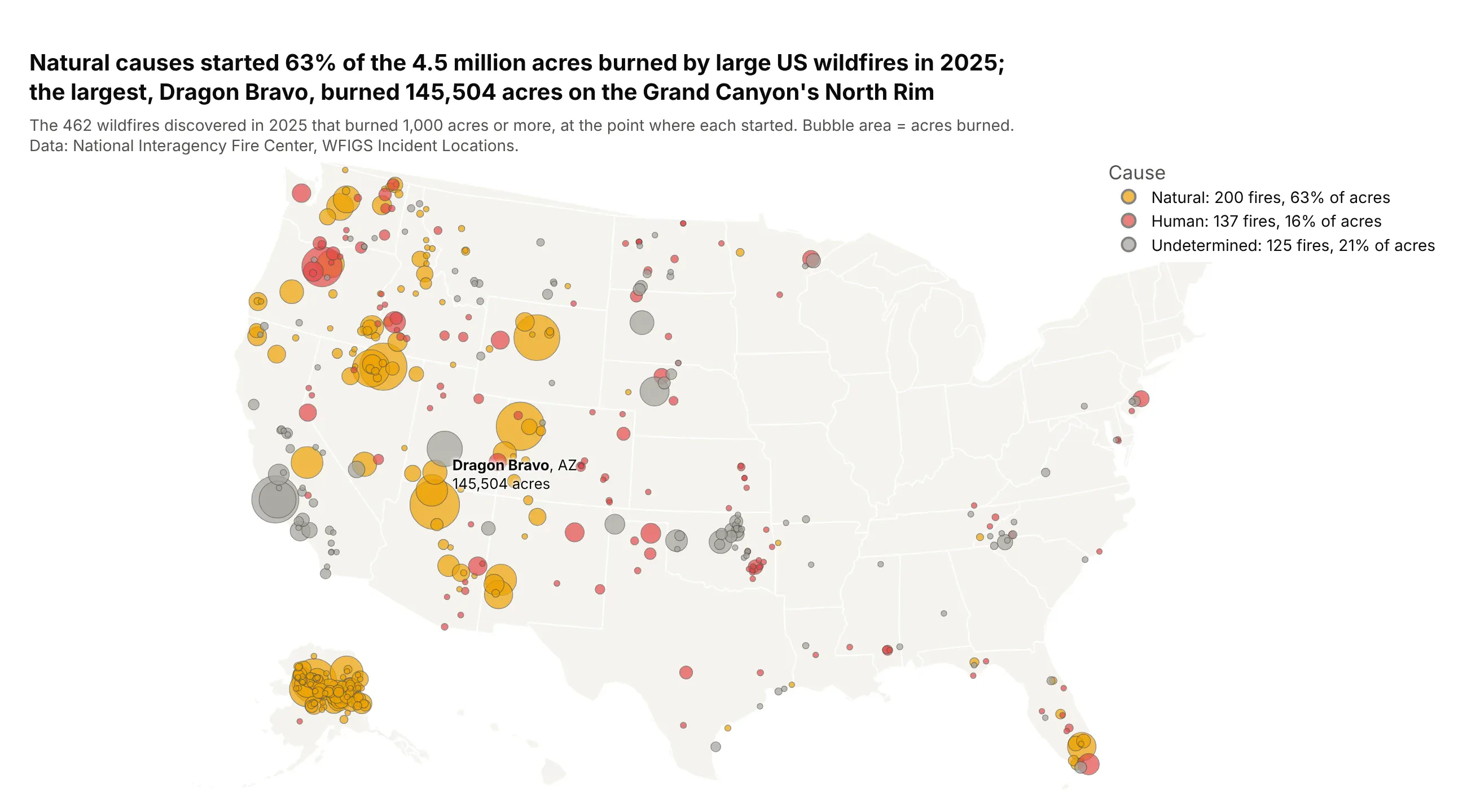
Natural causes started 63% of the 4.5 million acres burned by large US wildfires in 2025. The largest, Dragon Bravo, burned 145,504 acres on the Grand Canyon's North Rim, and Alaska burned 979,217 acres, more than any other state. Data: National Interagency Fire Center, WFIGS Incident Locations.

Tip: a dark outline at 0.6 pixels separates bubbles of the same color where fires overlap, as in Nevada and Oregon.

5. A decade of coal plant retirements

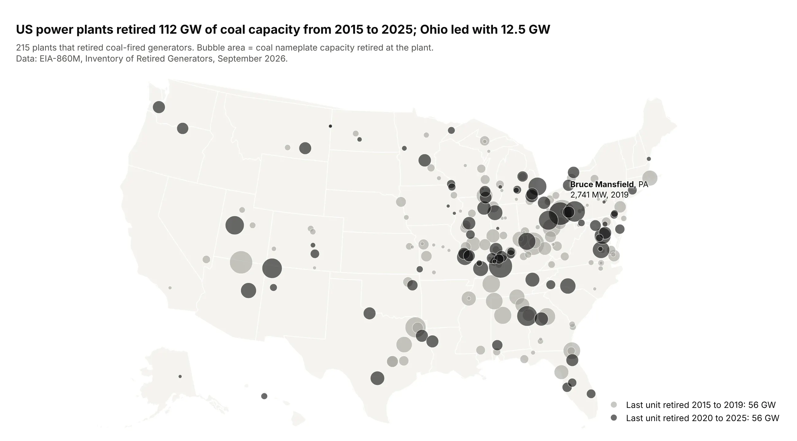
US power plants retired 112 GW of coal capacity from 2015 to 2025, half by 2019 and half since, and Ohio led with 12.5 GW. Homer City in Pennsylvania retired 2 GW of coal in 2024 and is now planning 4.4 GW of gas, the third-largest bubble in the main example. Data: EIA-860M, Inventory of Retired Generators, September 2026.

Tip: color by period instead of by category to add time to a static bubble map.

6. Counties that gained and lost people

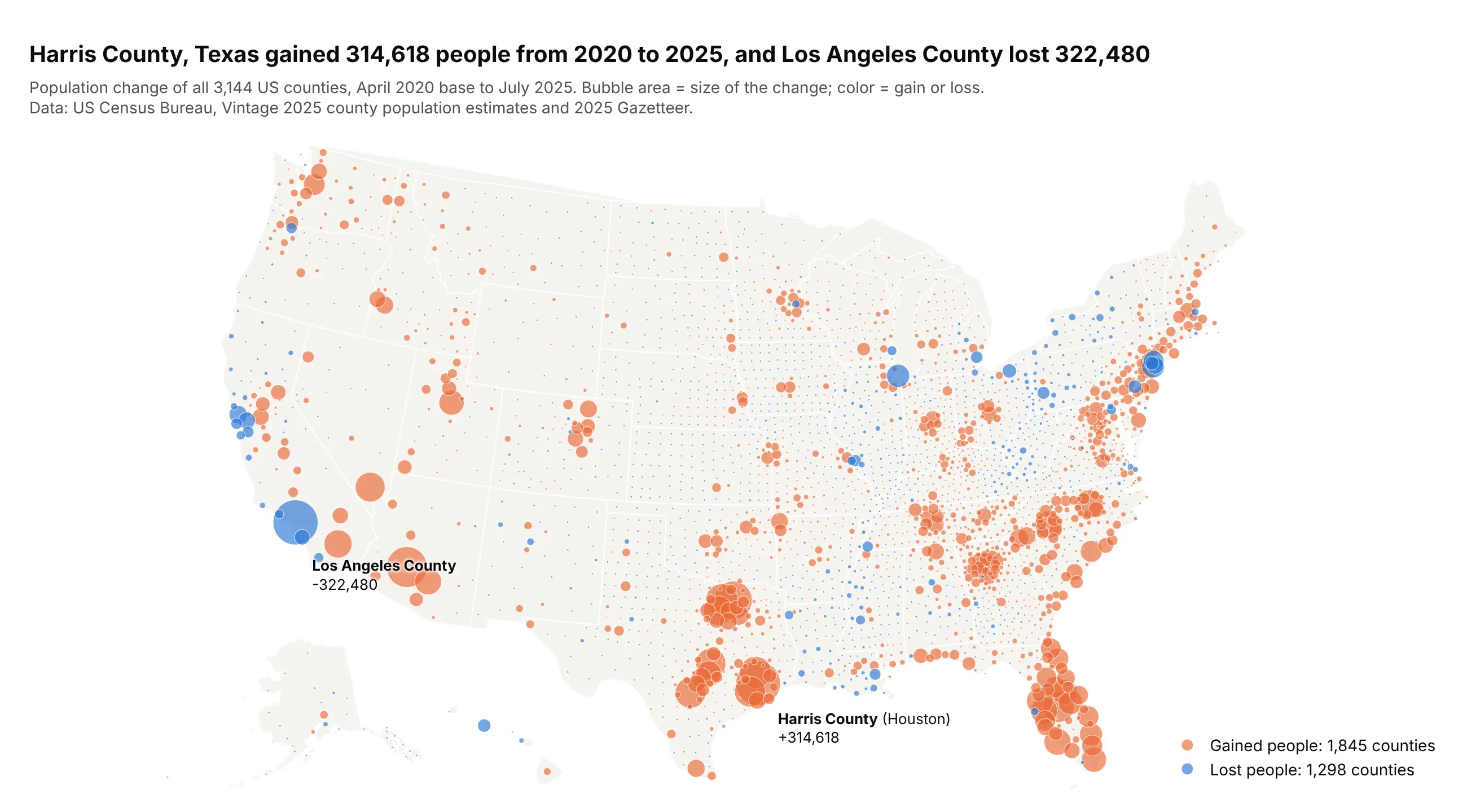
Harris County, Texas gained 314,618 people from 2020 to 2025, and Los Angeles County lost 322,480. 1,845 counties gained people and 1,298 lost. Data: US Census Bureau, Vintage 2025 county population estimates and 2025 Gazetteer.

Tip: size by the absolute change and color by its sign, because a bubble can't have a negative area.