
Chris Parmer
October 24, 2026
Choropleth Maps - A Complete Guide
TL;DR
- A choropleth map colors each region (a country, state, county or any shape you have) by a value for that region, so you can see where a rate is high and whether the high values cluster.
- Choropleth maps are also known as filled maps, and are similar to proportional symbol maps, cartograms and hexbin maps.
- Map rates, not counts. A map of totals mostly shows where people live, so divide by population, area or another base first.
- How you split the values into colors (a continuous scale, equal intervals, quantiles or natural breaks) changes the map more than any other choice.
- Any coding agent can make one with Plotly in a minute. In Python it's px.choropleth(df, locations="iso3", color="rate").
What is a choropleth map?
Choropleth maps look like this:
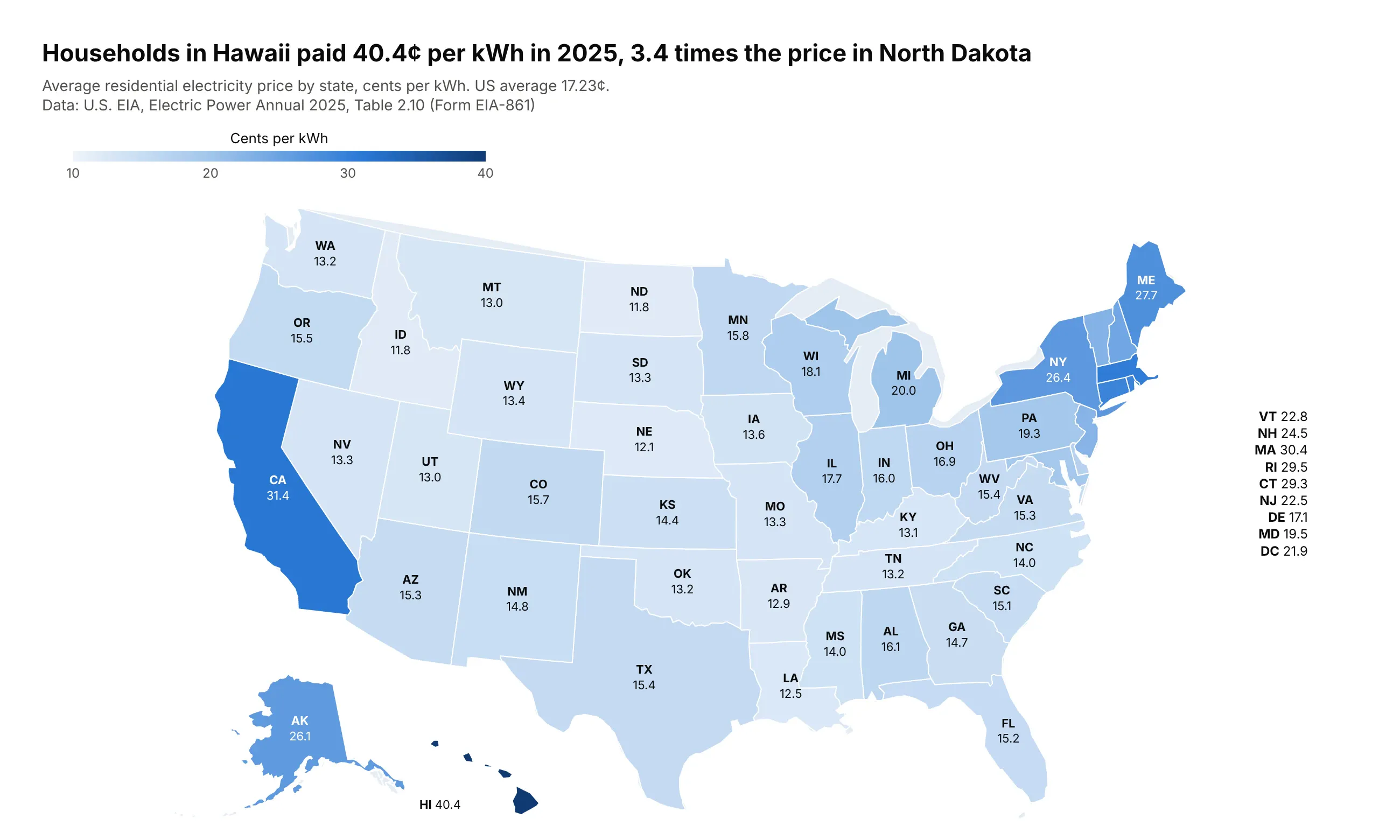
Data: U.S. EIA, Electric Power Annual, Table 2.10 (2025).
How do you read a choropleth map? In the example above, notice these things:
- Each state is filled with one color from the scale at the top, so the color stands for the average price its households paid per kWh in 2025, from nearly white for the cheapest states to dark blue for the most expensive.
- Look for clusters before single states. The ten most expensive states are the six in New England, New York, California, Alaska and Hawaii, while the states down the middle of the country, from Idaho and North Dakota to Louisiana, are all cheaper than the US average.
- The darkest shade belongs to Hawaii at 40.4¢, so one state sets the top of the scale and most of the others share its pale lower half.
- The number on each state is there because readers can't hover over a static image, and the small Northeastern states that have no room for a label are listed to the right of the map.
- Watch out for size. Texas and Montana catch the eye because they are big, while Massachusetts, the third most expensive state, is almost too small to see, and a state's land area has nothing to do with its price.
It's often used for charts like these:
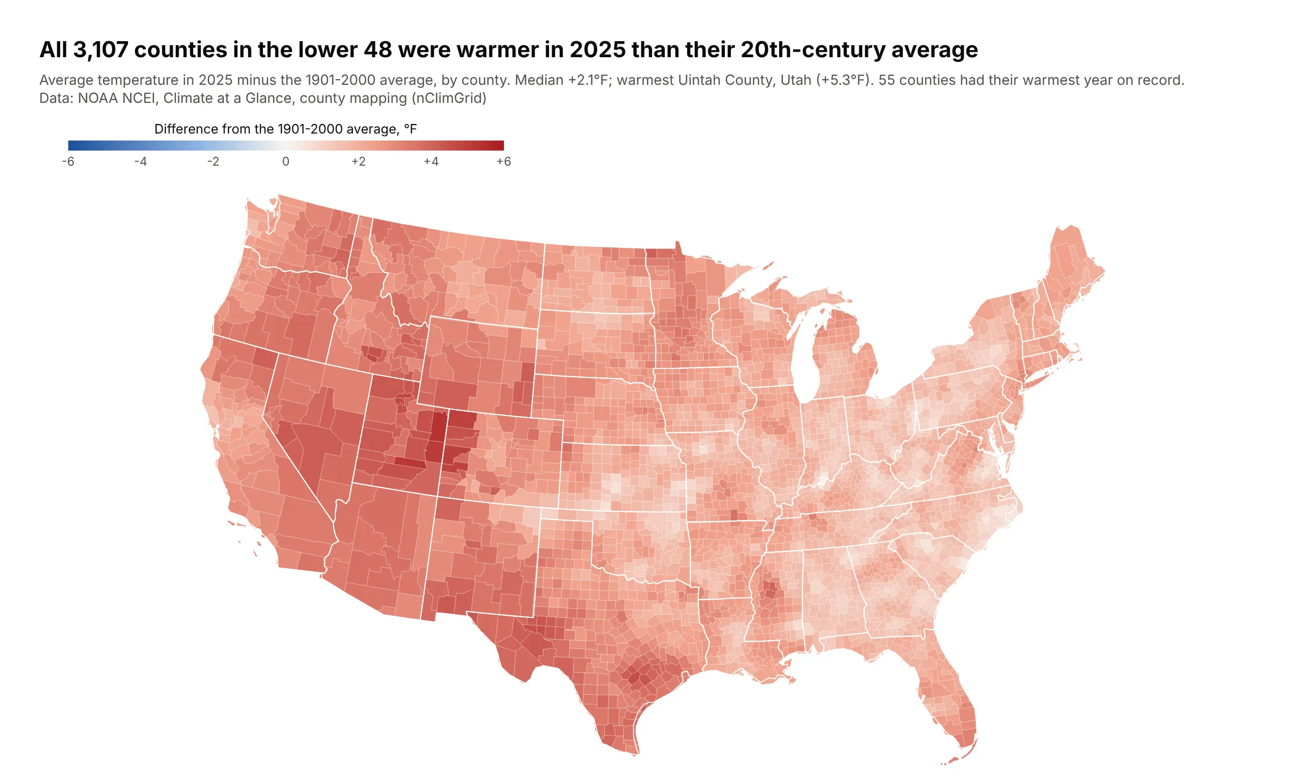
A climate measure by county. All 3,107 counties in the lower 48 were warmer in 2025 than their 20th-century average, by a median of 2.1°F, and the diverging scale is held at zero so the missing blue is the finding. Data: NOAA NCEI, Climate at a Glance, county mapping.
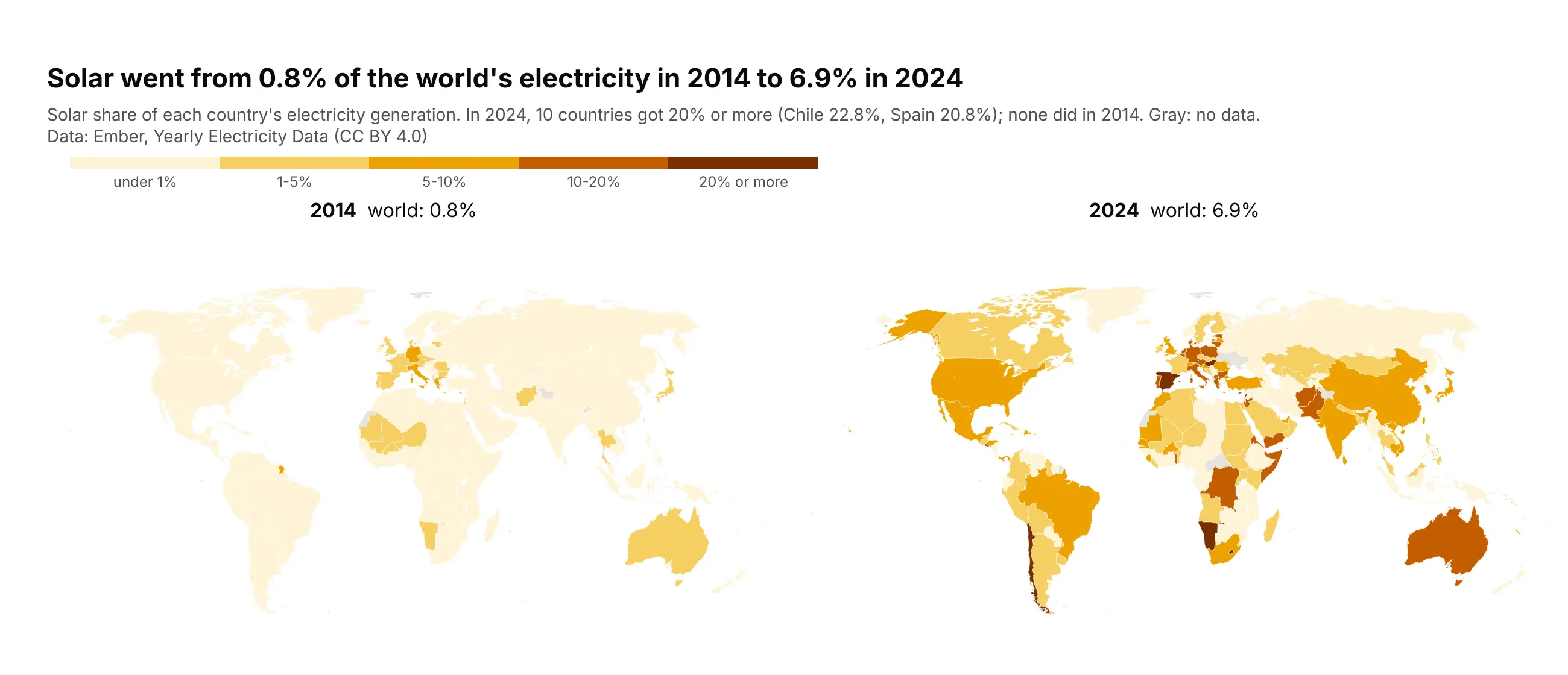
A share by country, compared across years. Solar went from 0.8% of the world's electricity in 2014 to 6.9% in 2024, and ten countries got 20% or more from solar in 2024, against none in 2014. Data: Ember, Yearly Electricity Data (CC BY 4.0).
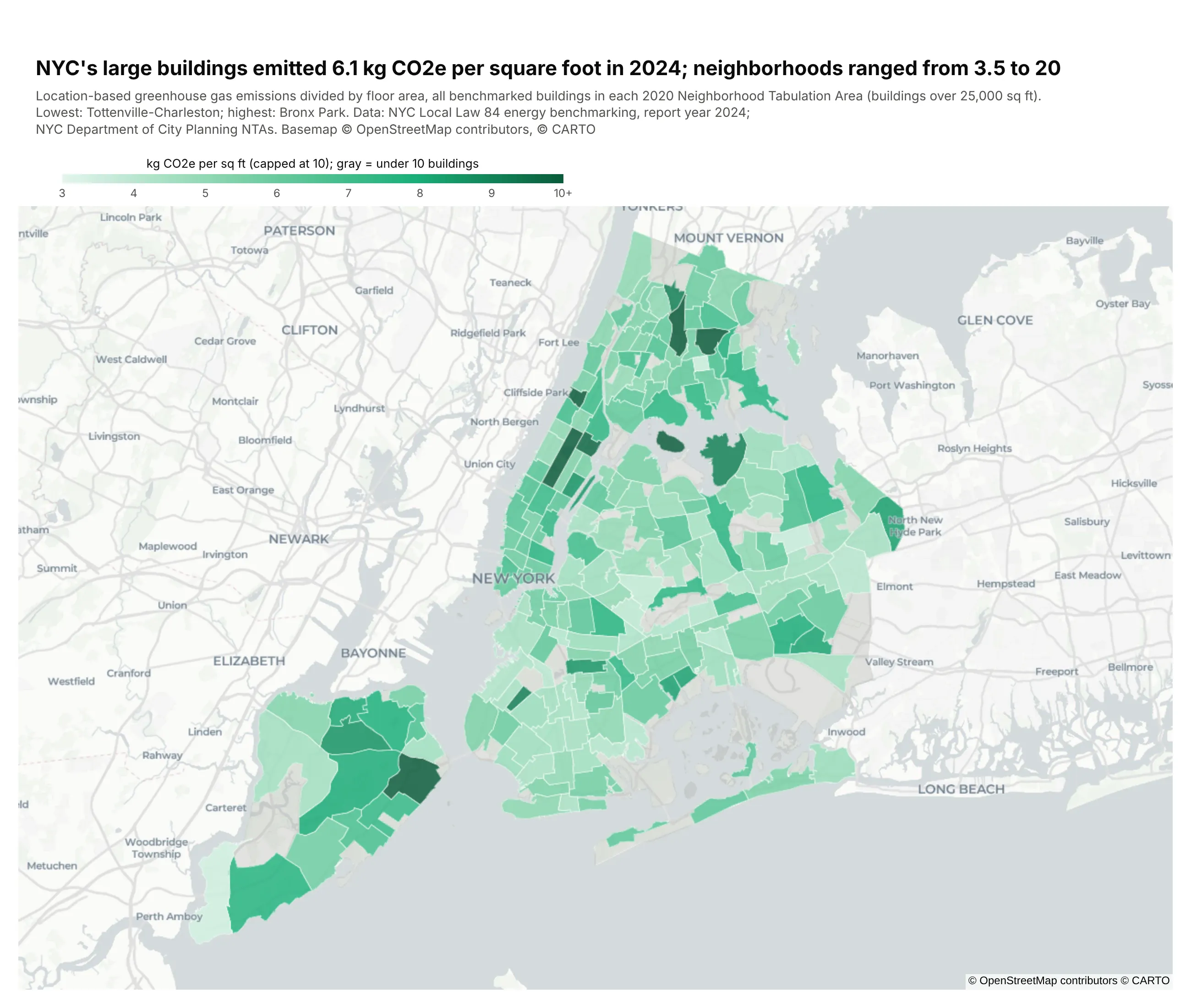
Your own regions on a street map. New York's large buildings emitted 6.1 kg CO2e per square foot in 2024, and neighborhood averages ran from 3.5 to 20, drawn from a custom GeoJSON with go.Choroplethmap. Data: NYC Local Law 84 benchmarking (29,420 buildings) and NYC Planning neighborhood boundaries.
A short history
The first choropleth is usually credited to Charles Dupin, whose 1826 map of France shaded each département by schooling, and the geographer John Kirtland Wright coined the word "choropleth" (from the Greek for area and multitude) in 1938. The ways to split values into colors came later: Walter Fisher published the optimal grouping in 1958 (doi:10.1080/01621459.1958.10501479), George Jenks made it the cartographer's "natural breaks", and Cynthia Brewer's tests of classification methods (doi:10.1111/1467-8306.00310) and her ColorBrewer palettes (doi:10.1179/000870403235002042) shaped how most maps are colored today.
Alternatives to a choropleth map
Here's the same 2025 overdose death data drawn four ways. Some are better for the question, some worse, some just different:
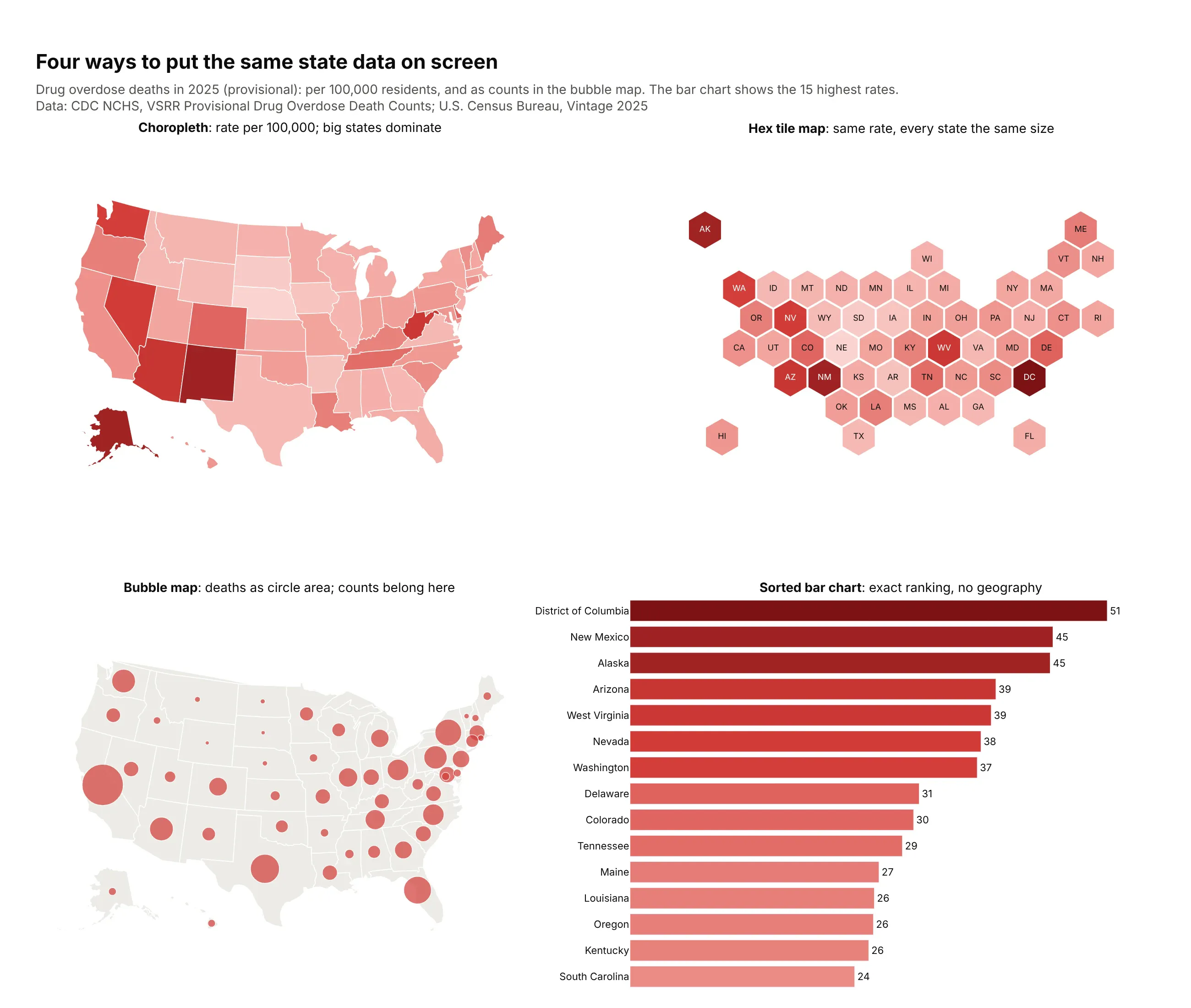
- Hex tile map (better when small regions matter). Every state gets the same size tile, so DC (51 deaths per 100,000, the highest rate) is as visible as Texas. You lose the real shapes, and readers need a moment to find their state. Example 7 below builds one.
- Bubble map (better for counts). Deaths are a count, so a circle sized by the number of deaths shows them without coloring whole states by how many people live there. Overlapping circles get hard to read in dense areas.
- Sorted bar chart (better for precise comparisons). People judge length on a shared baseline more accurately than color or area, as Cleveland and McGill (1984) measured, so use bars when the ranking matters more than the geography. You lose the clusters: the map shows that the highest rates sit in the Southwest and Appalachia.
- Choropleth (works well for rates). It's the right choice when you have one rate per region and the question is where. Big, empty regions get the most ink whatever their value, which is why the election map in example 10 fades counties by voter density.
How to make a choropleth map
With AI
ChatGPT, Claude Code, GitHub Copilot, Cursor and other AI tools are excellent at writing Plotly code. Name Plotly in the prompt, say what the regions are and what to divide by, and list the checks you want:
Make a plotly county choropleth from rates.csv(columns: fips as a 5-digit string, county, state, cases, population).- Map cases per 100,000 people, not cases.- Geometry: Census cartographic boundary file cb_2023_us_county_20m, converted to GeoJSONwith the 5-digit GEOID as each feature's id; round coordinates to 3 decimals.- Five quantile classes on a single-hue scale; colorbar ticks show each class range.- Counties with no row or fewer than 1,000 people: a gray layer, explained in the subtitle.- White state borders on top; hide the base map; albers usa projection.- Inter font, white background, a title that states the main takeaway with a number.- Print every data row whose fips matches no feature, and every feature with no data.- Save as map.html (check it is under 5 MB) and a PNG at 2x scale.
The matching check is worth keeping in every choropleth prompt. Plotly silently skips rows whose key doesn't match a feature, so a typo or a dropped leading zero just leaves a region blank.
With Plotly Studio
Plotly Studio is a desktop app where you point an AI at a dataset and it builds charts and a Dash app around your questions. Ask for a choropleth by naming the regions, the rate and the coloring:
Show a county choropleth of mortgage denial rates, with counties under 30 applications in gray and five natural-breaks classes on a light-to-dark red scale. Add a dropdown to switch between home purchase and refinance loans.
Make a choropleth map in Python or JavaScript
This is the code AI tools write under the hood. In Python, Plotly has the shapes of countries and US states built in, so you only need the codes:
import plotly.express as pxdf = px.data.gapminder().query("year == 2007")fig = px.choropleth(df, locations="iso_alpha", color="lifeExp",projection="natural earth", color_continuous_scale="Blues")fig.show()
For US counties or any other regions, pass a GeoJSON with geojson= and say which property holds the id with featureidkey= (the FAQ below has a county example).
In JavaScript, plotly.js takes the same codes and values. This draws the 2025 household electricity prices from the map at the top of this page:
<div id="chart"></div><script src="https://cdn.plot.ly/plotly-4.1.1.min.js"></script><script>const cents = {AK: 26.11, AL: 16.09, AR: 12.87, AZ: 15.26, CA: 31.35, CO: 15.69, CT: 29.31, DC: 21.92,DE: 17.15, FL: 15.21, GA: 14.74, HI: 40.4, IA: 13.62, ID: 11.83, IL: 17.67, IN: 15.96,KS: 14.44, KY: 13.13, LA: 12.52, MA: 30.41, MD: 19.53, ME: 27.69, MI: 20.03, MN: 15.83,MO: 13.3, MS: 14.03, MT: 12.99, NC: 14.0, ND: 11.82, NE: 12.05, NH: 24.53, NJ: 22.48,NM: 14.85, NV: 13.26, NY: 26.39, OH: 16.9, OK: 13.21, OR: 15.46, PA: 19.29, RI: 29.48,SC: 15.12, SD: 13.32, TN: 13.22, TX: 15.4, UT: 13.02, VA: 15.28, VT: 22.79, WA: 13.17,WI: 18.08, WV: 15.39, WY: 13.37};Plotly.newPlot("chart", [{type: "choropleth",locationmode: "USA-states",locations: Object.keys(cents),z: Object.values(cents),colorscale: "Blues",reversescale: true,marker: {line: {color: "white", width: 1}},colorbar: {title: {text: "Cents per kWh"}}}], {geo: {scope: "usa", projection: {type: "albers usa"}}});</script>
Share it
Every Plotly chart has a Share chart button (the cloud icon in its toolbar) that uploads it to Plotly Cloud and gives you a link. Only you can see it until you change its visibility.
For a live app, put the chart in a Dash app and publish it with the Plotly Cloud CLI. Coding agents can run these commands for you:
pip install "dash[cloud]"plotly user loginplotly app publish
If your data has to stay in your own cloud or data center, publish to Dash Enterprise instead.
Dos and don'ts
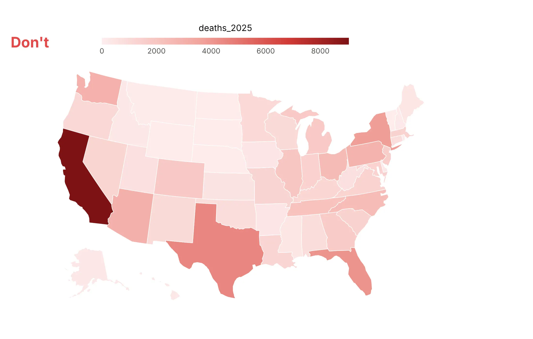
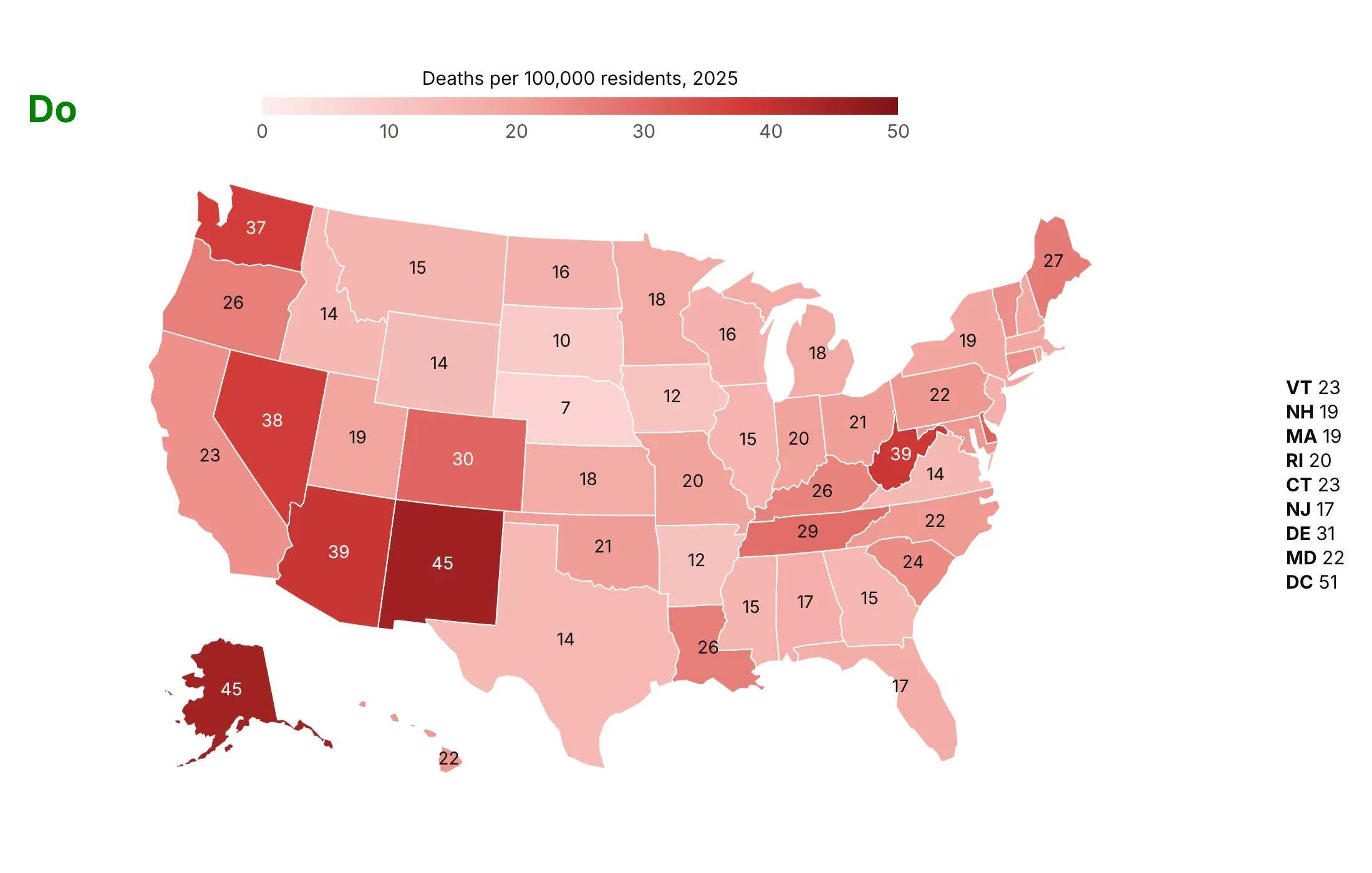
Most of the work in a choropleth is in two decisions: what to divide by, and how to split the values into colors. Here is the 2025 overdose data both ways, with the same color scale.
Don't map raw counts. California, Texas and Florida come out darkest because they're the most populous states, the colorbar shows the column name and unformatted numbers, and nothing tells a reader of a static image what any state's value is:
Do map deaths per 100,000 residents, title the colorbar in words and print each state's rate, with the small Northeastern states listed beside the map. Now the highest rates show up where they are: DC (51), New Mexico (45) and Alaska (45):
Pick the color classes for the question
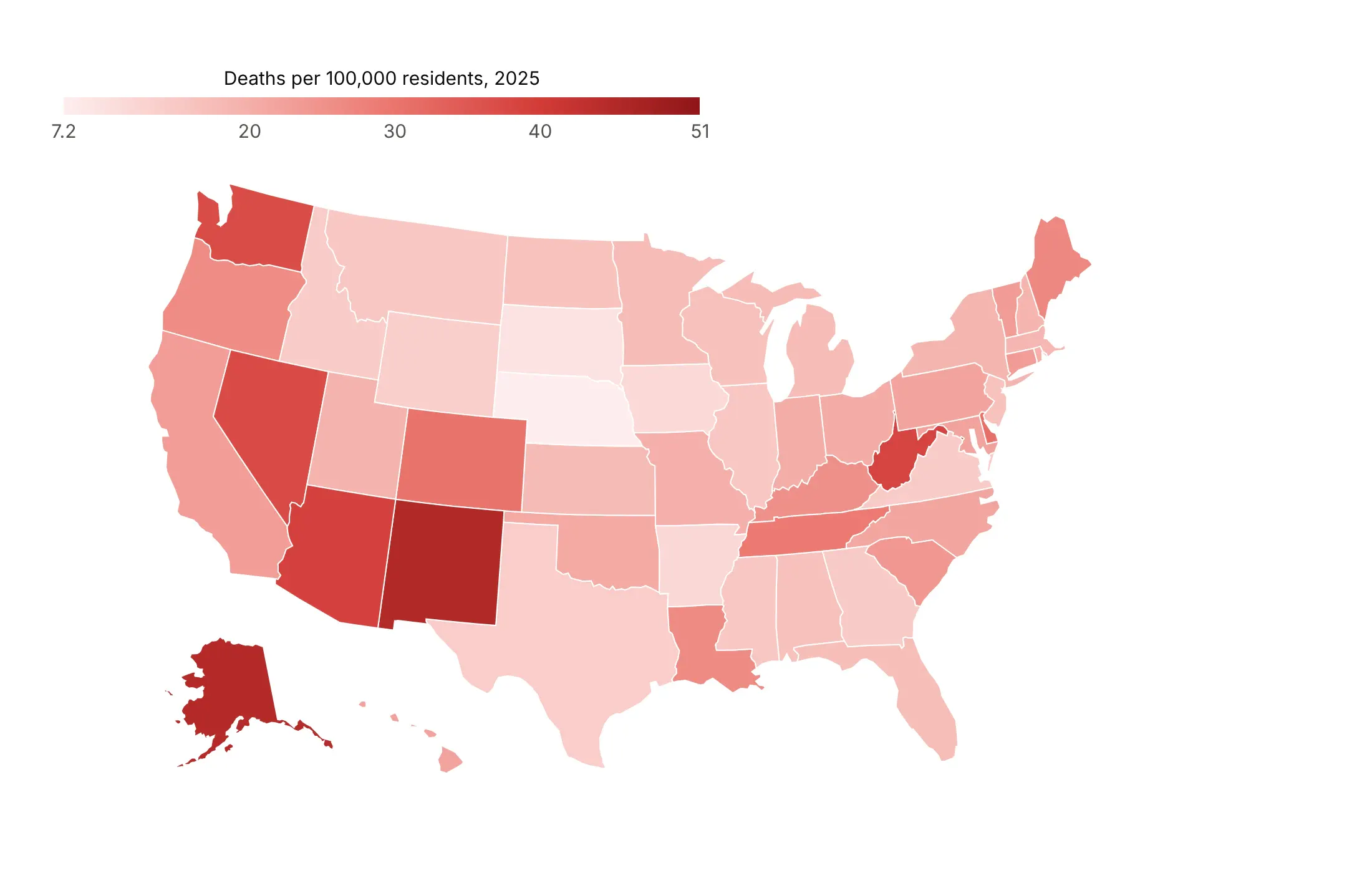
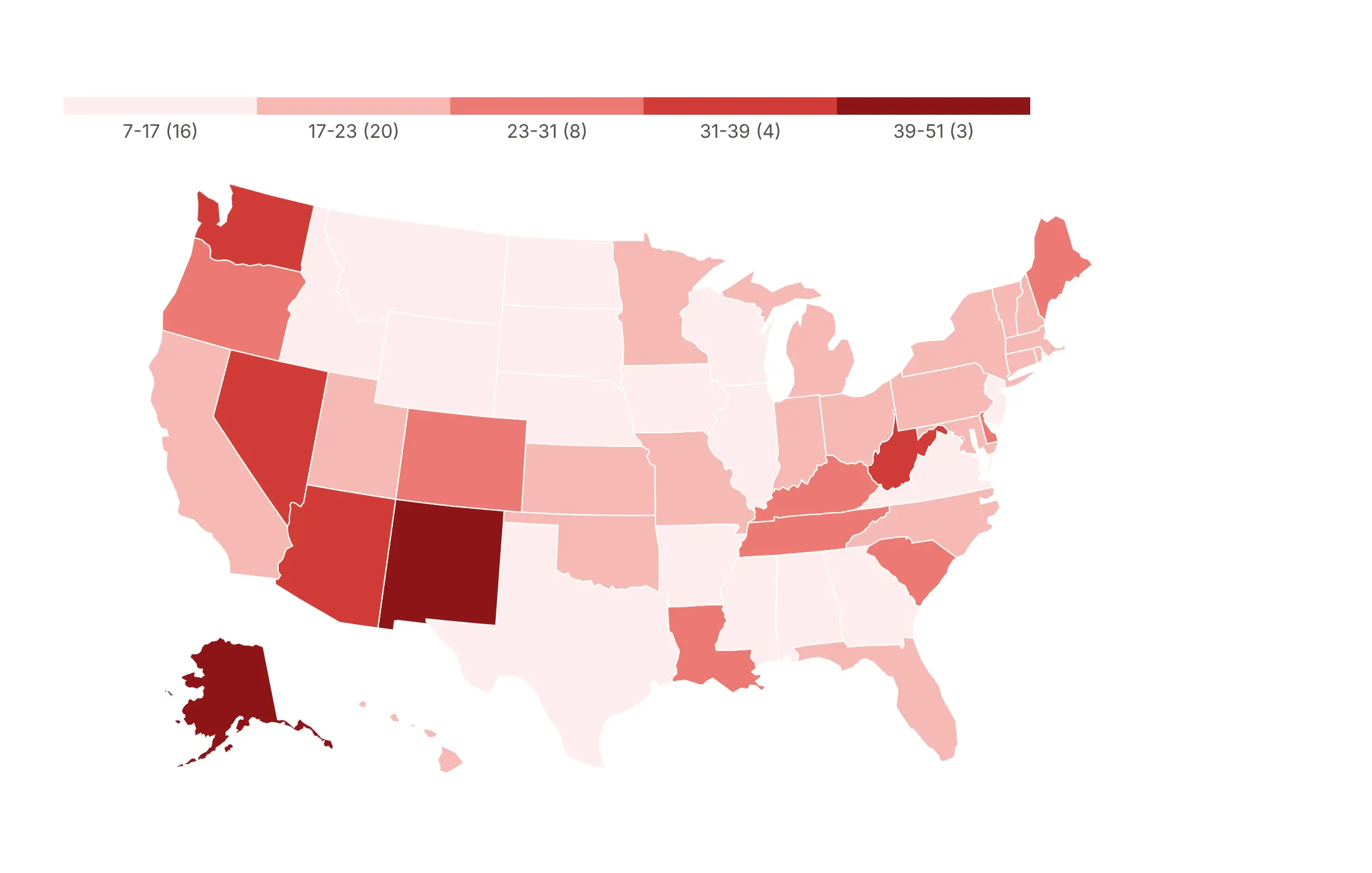
Once you have a rate, the way you split it into colors changes the map again. Here are the same 51 overdose death rates four ways. The numbers in parentheses are how many states fall in each class.
Continuous scale. It is honest about every value, but states 3 or 4 points apart look nearly the same, so it's best when the exact value matters more than groups.
Equal intervals. Each class covers the same range, which is easy to explain, but skewed data leaves most states in the two lightest classes (37 of 51 here).
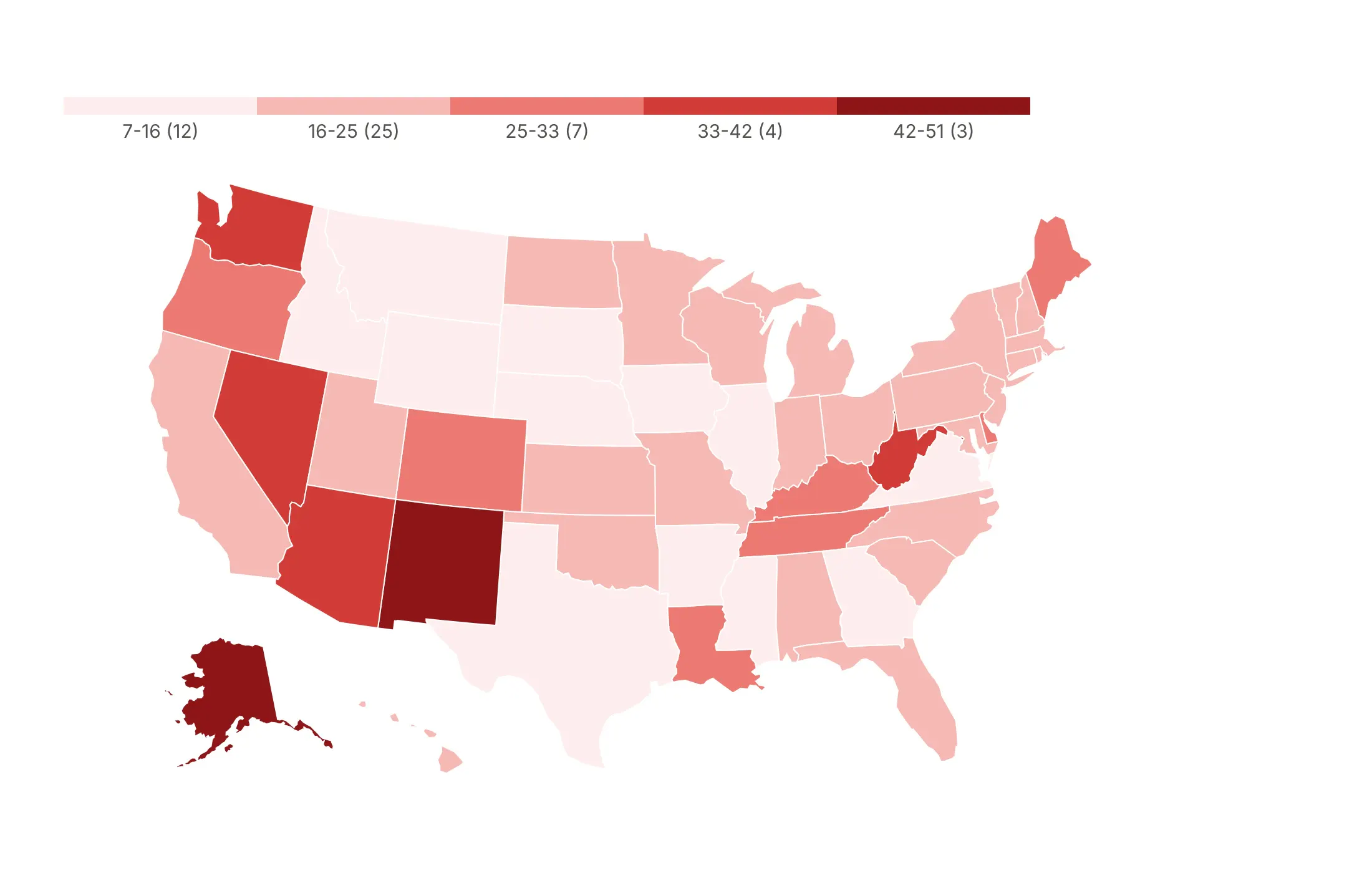
Quantiles. Each class holds the same number of states, about 10, which is good for ranking but puts states with 27 and 51 deaths per 100,000 in the same color.
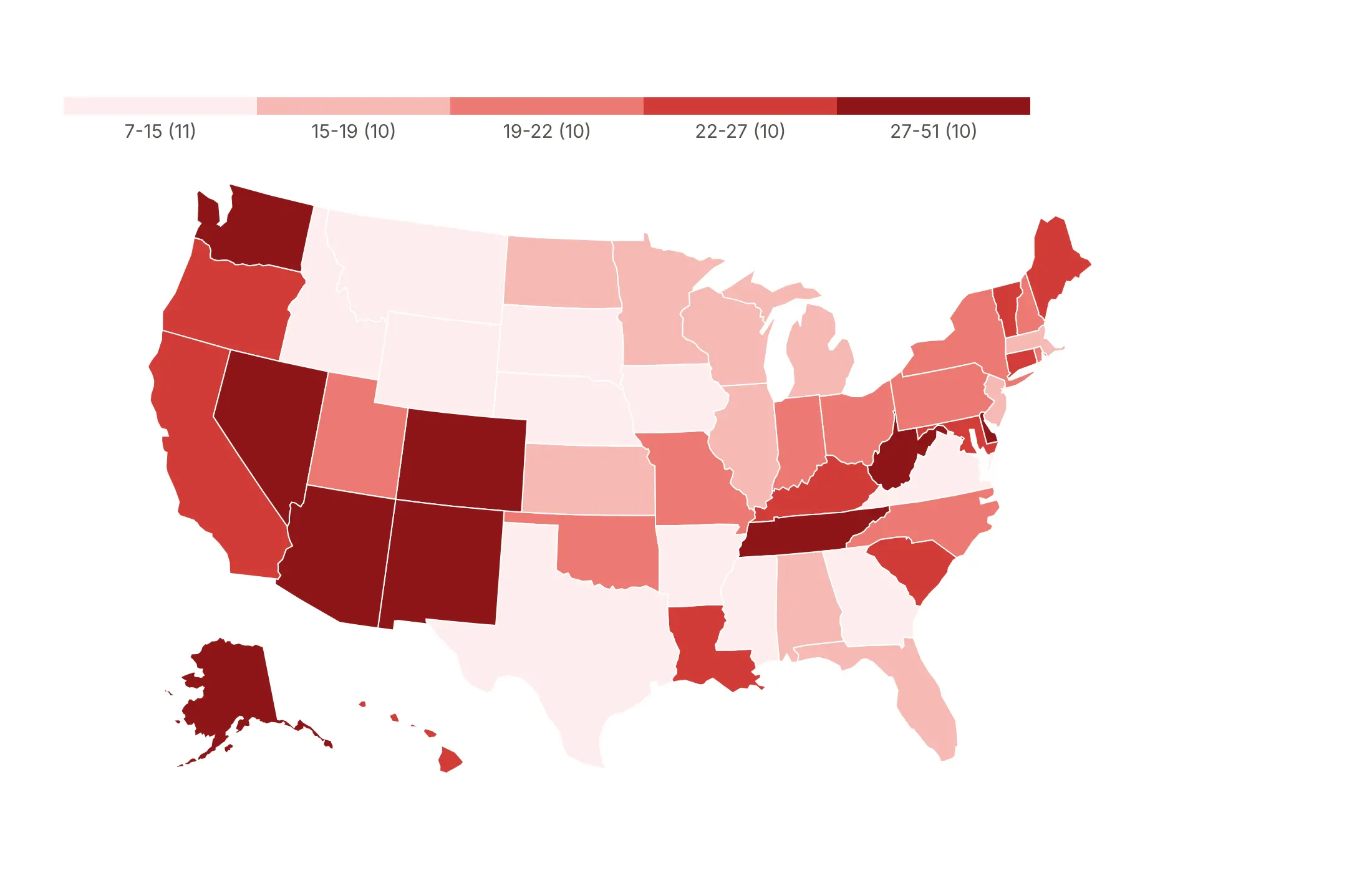
Natural breaks (Jenks). The edges fall in the gaps in the data (16.7, 23.3, 30.9 and 39.1), which suits data with clusters.
Checklist
Do
- Normalize: per capita, per area, per household, or a share of a total.
- Write a title that states the takeaway with a number, and name the source and year in the subtitle.
- Use a diverging scale only around a meaningful midpoint (zero, a target, the national average) with zmid.
- Show missing data as its own gray, and say what gray means.
- Cap outliers with zmin and zmax, and say so on the colorbar ("10+").
- Use albers usa for US maps and Natural Earth or Robinson for world maps.
Don't
- Map counts unless the count is the point and the regions are the same size.
- Use a rainbow scale, whose bright bands create boundaries that aren't in the data.
- Let "no data" look like zero. Plotly leaves unmatched regions blank, which reads as low.
- Use Mercator for a world map, which makes Greenland look as big as Africa, a continent 14 times larger.
Options to customize
These are the go.Choropleth, go.Choroplethmap and px.choropleth options that matter most. The full list is in the Plotly choropleth documentation.
- locations: the key of each row (a code, a name or a GeoJSON feature id).
- locationmode: ISO-3, USA-states, country names or geojson-id. Built-in countries and states need no GeoJSON.
- geojson, featureidkey: your own shapes, and the property that holds the id (id or properties.GEOID), for counties, grid regions or neighborhoods.
- z (color in px): the value of each region.
- zmin, zmax, zmid: the range of the color scale and its midpoint; cap outliers and center diverging scales.
- colorscale: the value-to-color mapping; repeat stops to make a stepped scale for classed maps.
- coloraxis (layout): one color scale shared by several maps, for small multiples.
- colorbar: position, orientation, tickvals and ticktext, for class labels such as "1,000-1,800".
- marker.line: border color and width, usually thin white lines.
- marker.opacity: fill opacity, one value per trace, for layers over a basemap.
- customdata, hovertemplate: extra fields in the hover, such as the counts behind a rate.
- showscale: hides the colorbar, for gray "no data" layers.
- geo.scope: world, usa, europe, asia, africa, north america or south america.
- geo.projection.type: albers usa, natural earth, robinson, orthographic, mercator and more.
- geo.projection.rotation: the center longitude and latitude, for Europe-centered or globe views.
- geo.fitbounds: "locations" zooms to the data, for custom GeoJSON and partial maps.
- geo.visible, showland, showsubunits: base map layers; hide them for county maps, or use gray land for "outside the data".
- geo.lataxis.range, geo.lonaxis.range: crop the map for a tight regional view.
- map.style, map.center, map.zoom (Choroplethmap): the tile basemap and view, for city maps with street context.
- facet_col, animation_frame (px): small multiples or an animation over a column.
More choropleth map examples
Ten more choropleth maps built from real public data in energy, finance, health and politics, each with its source, the technique that makes it work and a prompt to rebuild it.
1. The largest source of electricity in each state
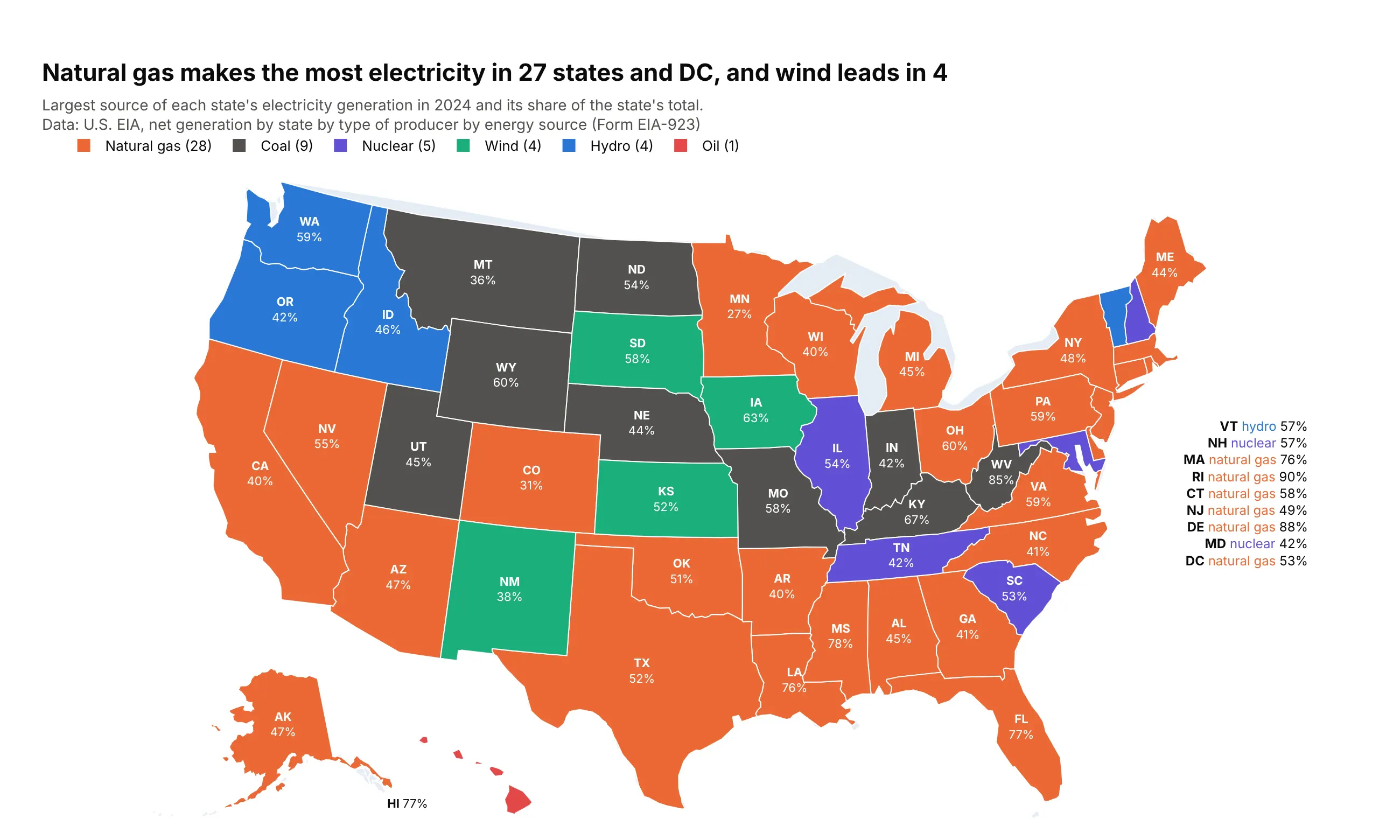
Natural gas generated the most electricity in 27 states and DC in 2024, coal in 9, nuclear and hydro in 5 and 4, and wind in 4, led by Iowa at 63%. Hawaii is the only state that runs mostly on oil. Data: U.S. EIA, net generation by state and energy source (EIA-923), 2024.
Tip: a categorical choropleth is one trace per category, each with a single-color colorscale and showlegend=True, and the legend counts the states.
Get the data from the U.S. EIA "Net Generation by State by Type of Producer by Energy Source" file(annual_generation_state.xls, eia.gov/electricity/data/state) and shape it into a table(columns: state_po, source, gen_mwh, share), 2024, total electric power industry.Build a plotly choropleth of each state's largest source: one go.Choropleth trace per source with afixed color (gas orange, coal dark gray, nuclear purple, wind green, hydro blue, oil red) and alegend that shows the number of states. Label each state with its code and share.
2. Utility-scale solar by county
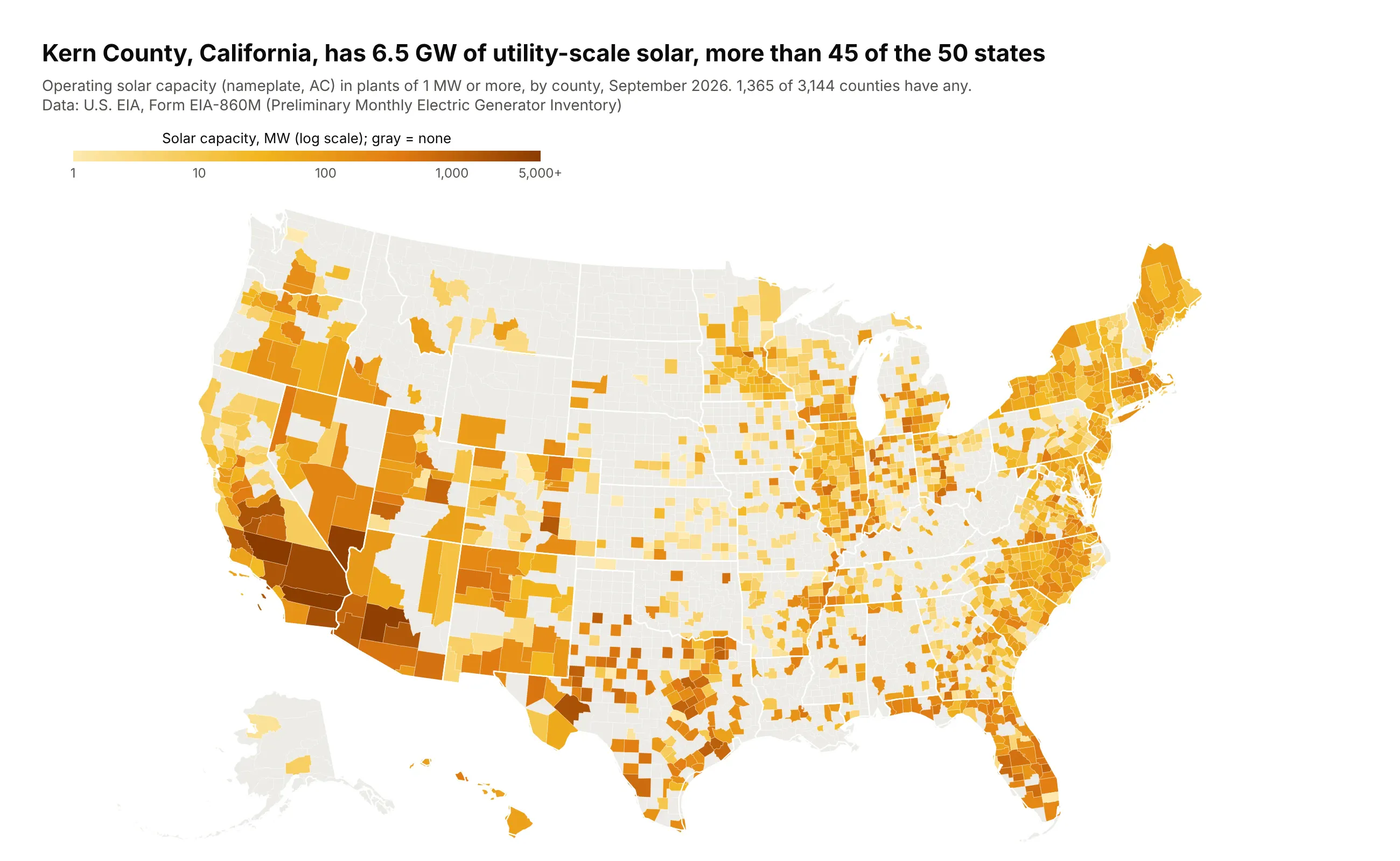
Kern County, California, has 6.5 GW of utility-scale solar, more than 45 of the 50 states. Only 1,365 of 3,144 counties have any, and capacity spans 1 MW to thousands, so the scale is logarithmic. Data: U.S. EIA, Form EIA-860M, September 2026.
Tip: color by np.log10(MW) and relabel the colorbar ticks as 1, 10, 100, 1,000, with zero in a separate gray trace.
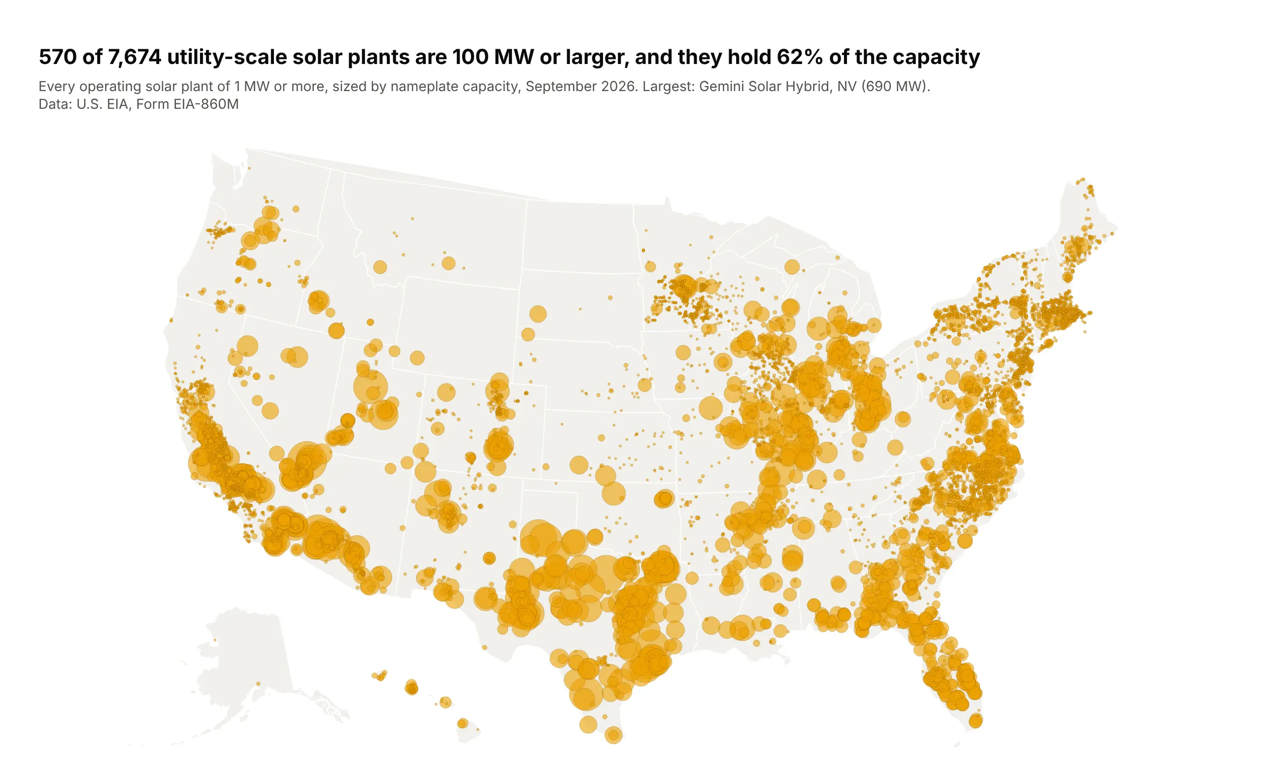
Get the data from the U.S. EIA Form EIA-860M generator inventory (latest month, eia.gov/electricity/data/eia860m),operating solar generators, and shape it into a county table(columns: fips, county, state_po, solar_mw, plants), placing each plant in a county by its latitude and longitude.Build a plotly county choropleth of solar_mw from a county GeoJSON keyed by FIPS. Color log10(solar_mw)with ticks at 1, 10, 100, 1,000 MW; counties with no solar in light gray; white state borders on top.Title: the largest county's GW and how many states it beats.
Another way to see it: capacity is a count, so a bubble per plant shows the same data without the big-county effect.
3. Wind and solar in each grid operator
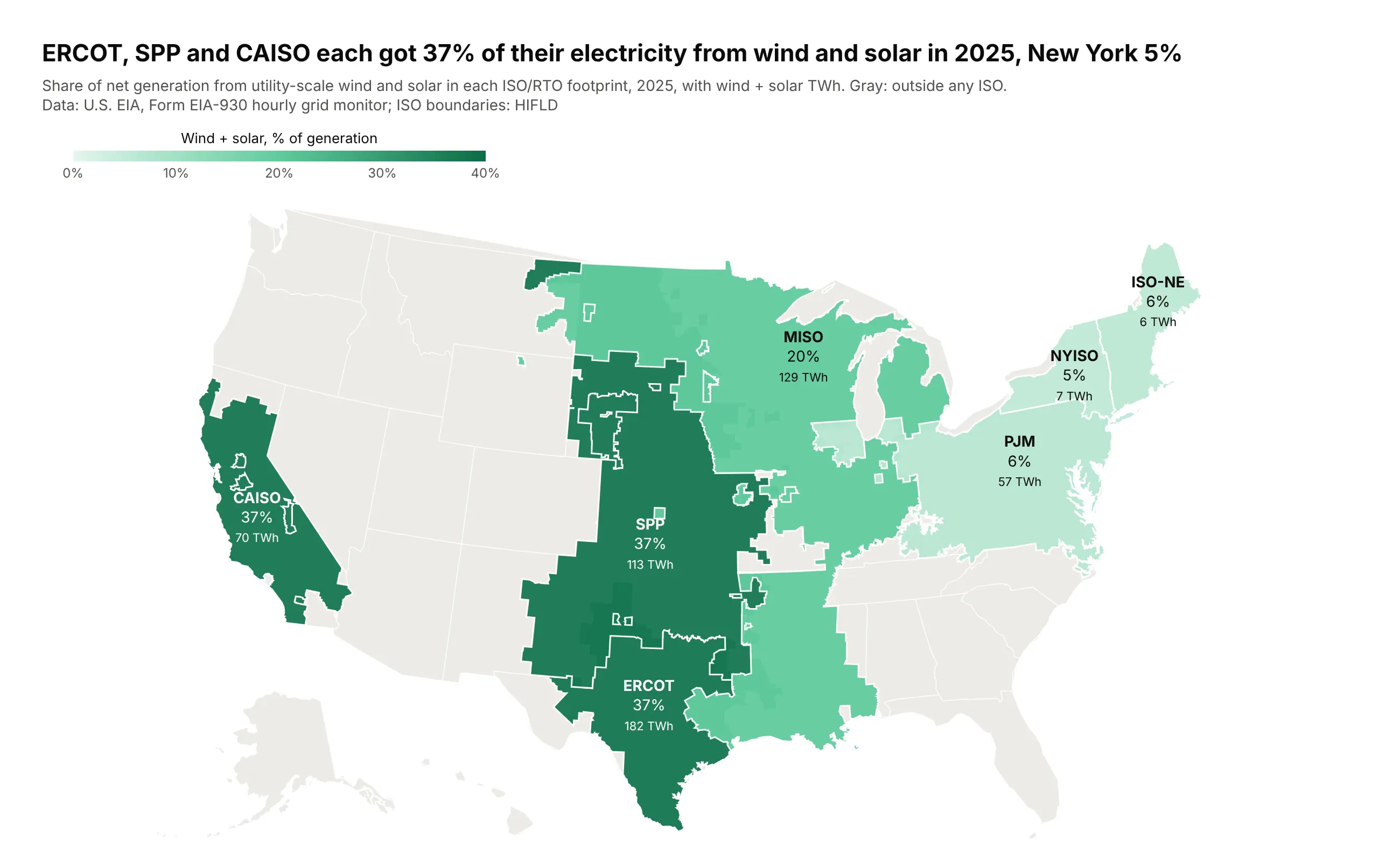
ERCOT, SPP and CAISO each got 37% of their 2025 electricity from wind and solar, against 5% in New York. Grid data comes by operator, not state, so the map uses the operators' own footprints from a custom GeoJSON. Data: U.S. EIA, Form EIA-930 (2025); boundaries from HIFLD.
Tip: draw the regions on a gray base map (showland, showsubunits) so areas outside every ISO read as "not in this data" rather than as low.
Get the data from the U.S. EIA Form EIA-930 hourly grid monitor six-month BALANCE files for 2025(eia.gov/electricity/gridmonitor) and the HIFLD "Independent System Operators" boundaries, and shape theminto a table (columns: iso, wind_twh, solar_twh, total_twh, share_wind_solar) and a GeoJSON with onefeature per ISO.Build a plotly go.Choropleth with geojson and featureidkey="id" on the albers usa projection, a grayland layer with white state lines underneath, and a green scale from 0 to 40%. Label each ISO with itsname, share and wind + solar TWh. Check that every outer ring is clockwise.
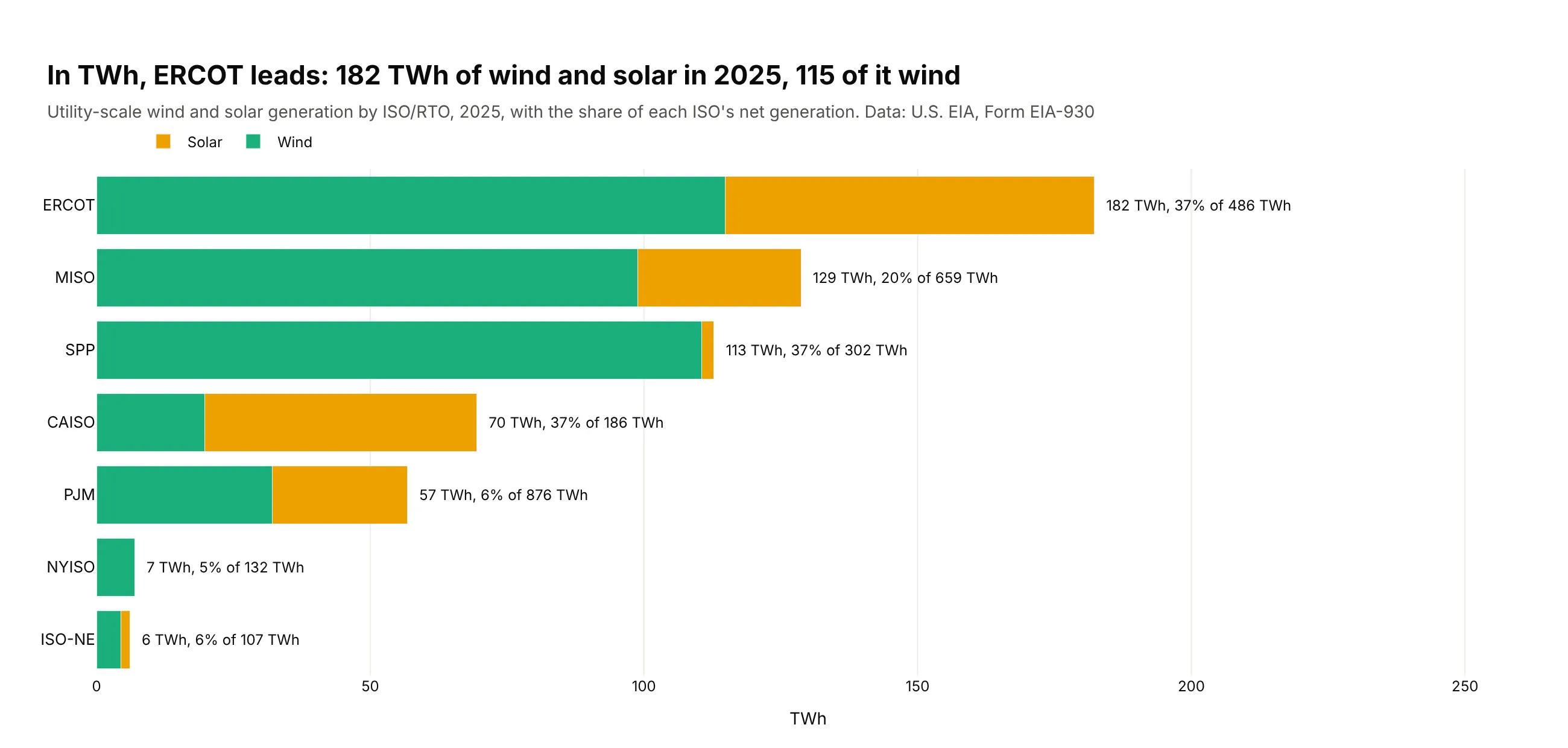
Another way to see it: in TWh, ERCOT's 182 TWh of wind and solar is more than any other ISO, 115 TWh of it wind.
4. Bank deposit concentration by county
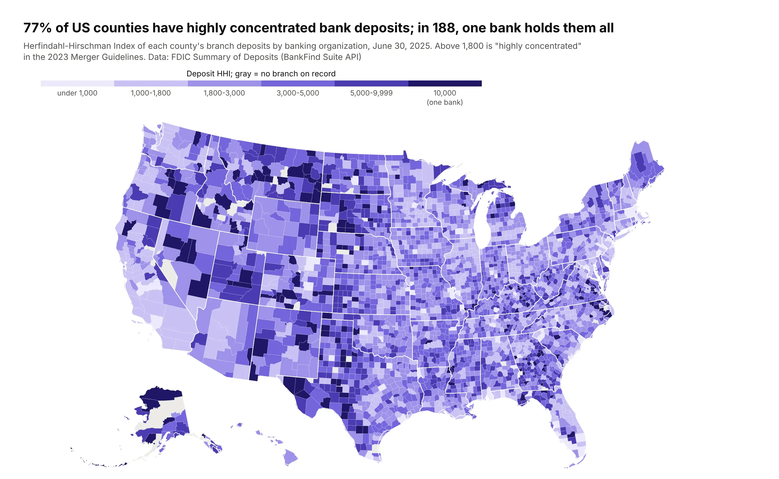
77% of US counties have highly concentrated bank deposits (an HHI above 1,800), and in 188 a single banking organization holds them all. Metro areas are the competitive ones. Data: FDIC Summary of Deposits, June 30, 2025.
Tip: take the class breaks from the rulebook (1,000 and 1,800 from the merger guidelines) rather than from the data, so each color has a meaning.
Get the data from the FDIC Summary of Deposits (BankFind Suite API, api.fdic.gov/banks/sod, YEAR 2025) andshape it into a county table (columns: fips, deposits_bn, branches, orgs, hhi, top_org, top_share),grouping branches by top holding company.Build a plotly county choropleth of hhi in classes under 1,000, 1,000-1,800, 1,800-3,000, 3,000-5,000,5,000-9,999 and 10,000, purple scale, counties with no branch in gray. Hover shows the largest bank.
5. Inflation around the world
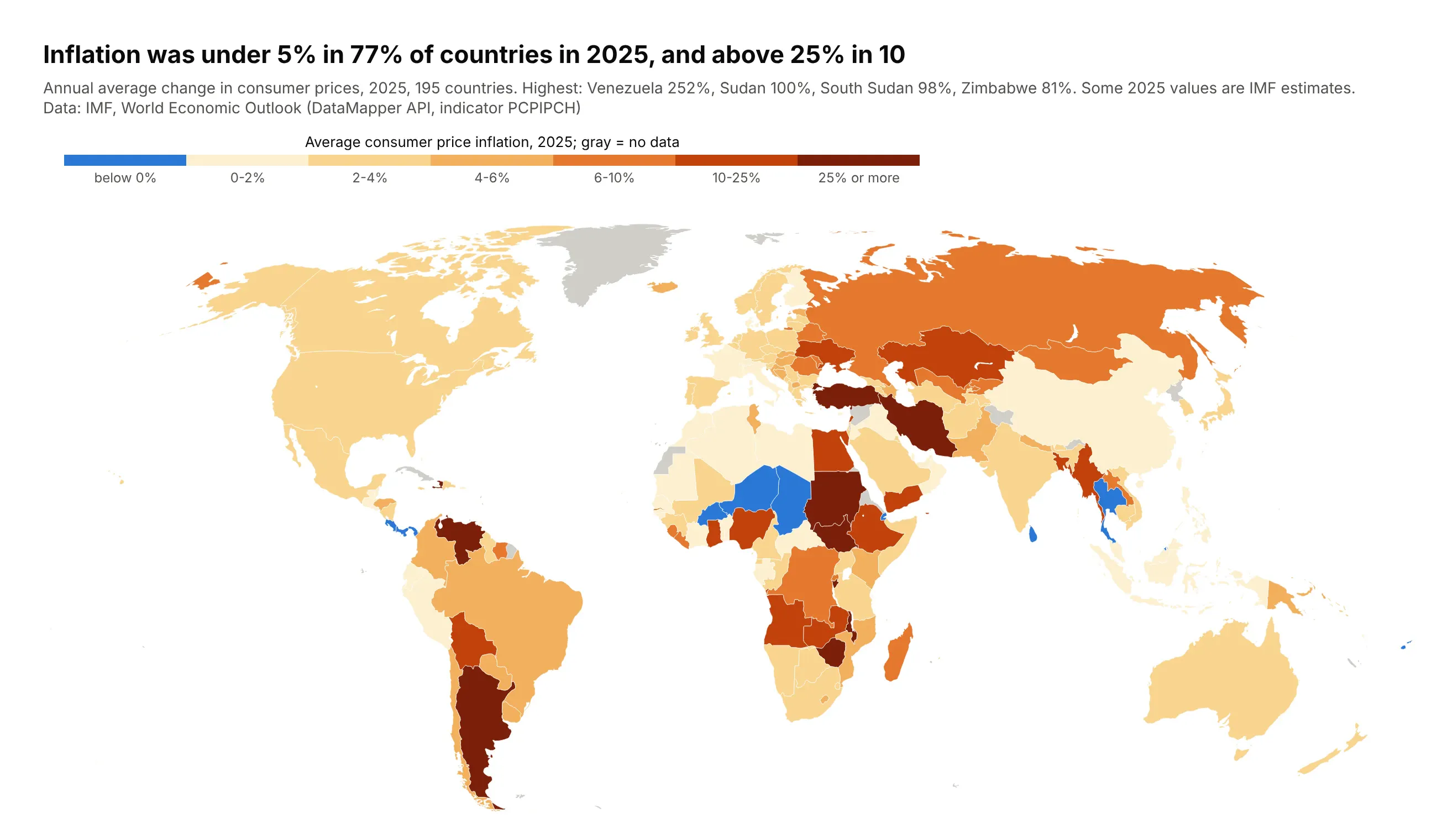
Inflation was under 5% in 77% of countries in 2025 and above 25% in 10, led by Venezuela at 252%. A linear scale from -5 to 252 would paint almost every country the same pale color. Data: IMF, World Economic Outlook.
Tip: hand-picked breaks (below 0, 2, 4, 6, 10, 25) with deflation in its own blue class.
Get the data from the IMF World Economic Outlook (DataMapper API, indicator PCPIPCH) and shape it into atable (columns: iso3, country, inflation_2025, inflation_2024).Build a plotly world choropleth (Robinson projection, ISO-3 codes) with classes below 0, 0-2, 2-4, 4-6,6-10, 10-25 and 25%+, blue for deflation and yellow to dark red above zero, gray land for no data.
6. Diabetes by county
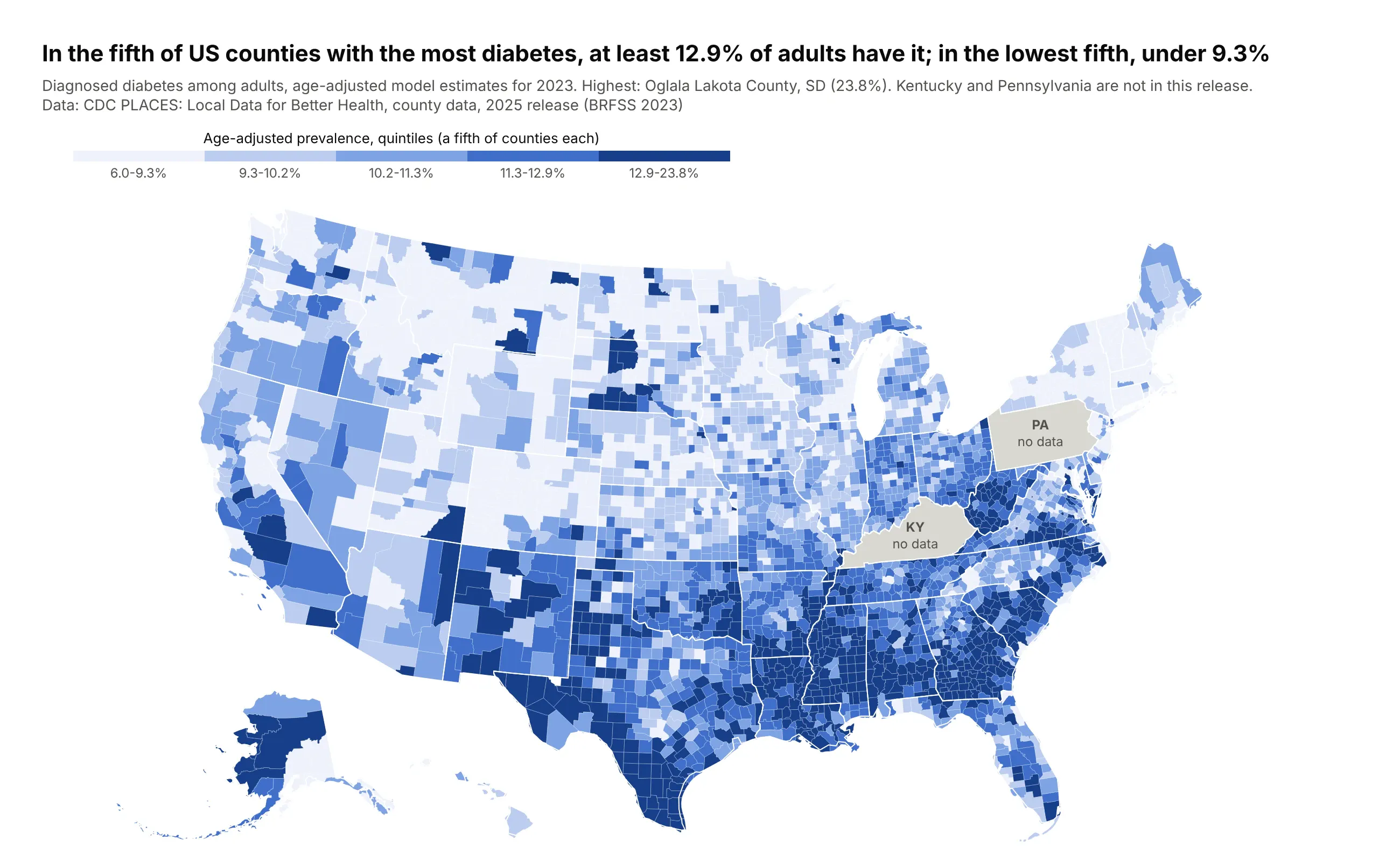
In the fifth of counties with the most diabetes, at least 12.9% of adults have it; in the lowest fifth, under 9.3%. The highest is Oglala Lakota County, South Dakota, at 23.8%, and Kentucky and Pennsylvania aren't in this release. Data: CDC PLACES, 2025 release (BRFSS 2023).
Tip: label missing states on the map itself, because a reader who sees an unlabeled gray state assumes it is low.
Get the data from CDC PLACES county data, 2025 release (data.cdc.gov swc5-untb, measure DIABETES, age-adjusted)and shape it into a table (columns: fips, county, state_po, diabetes_pct, low_ci, high_ci).Build a plotly county choropleth in quintiles (pd.qcut) on a blue scale with ranges on the colorbar;states with no data in gray with a "no data" label. Hover shows the confidence interval.
7. Change in overdose deaths, on a hex tile map
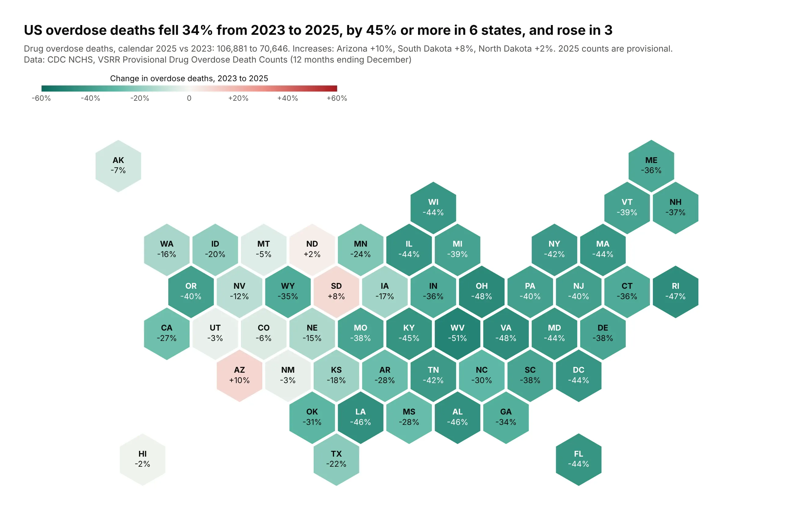
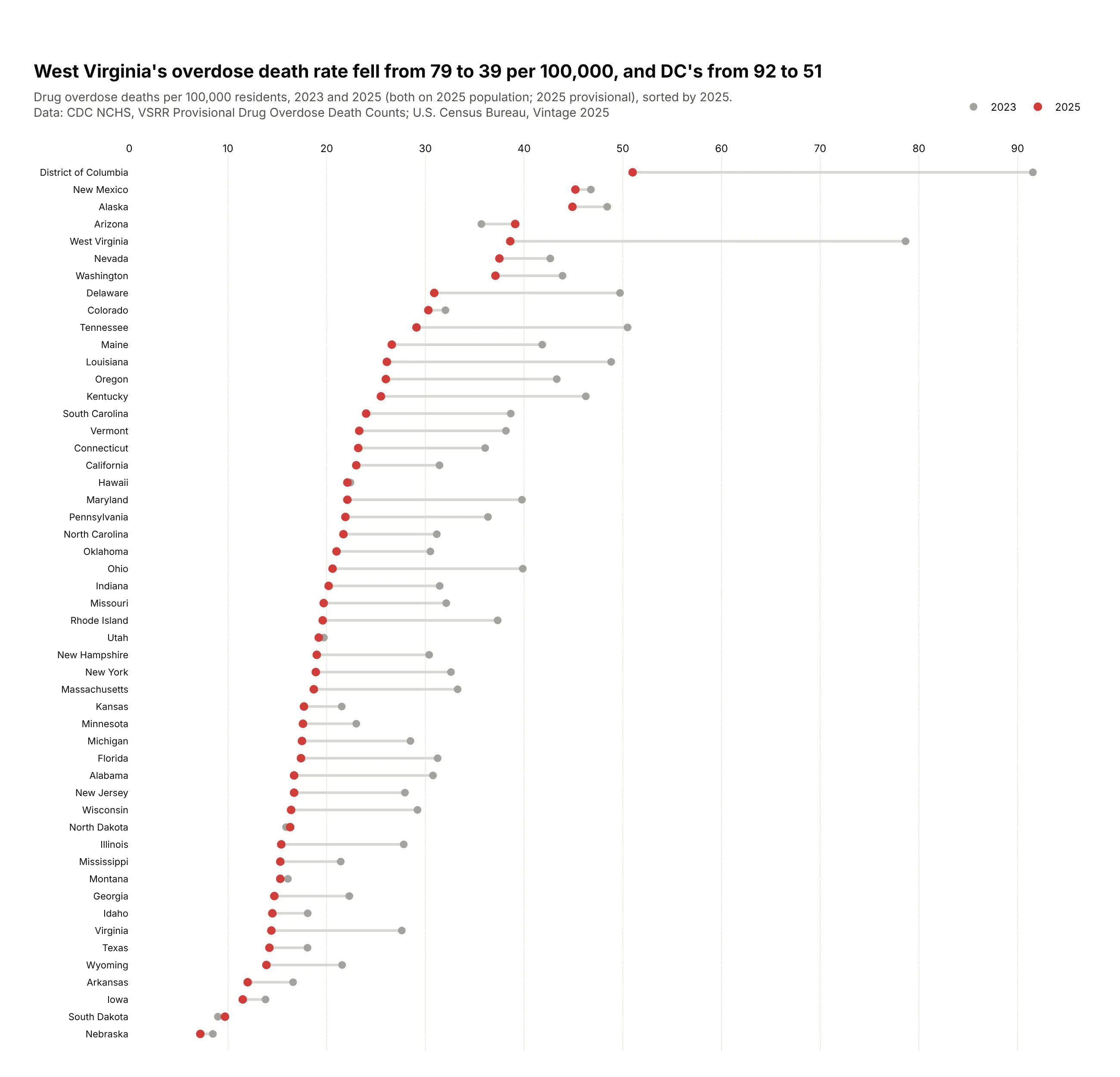
US overdose deaths fell 34% from 2023 to 2025, from 106,881 to 70,646, by 45% or more in six states, and rose in three: Arizona, South Dakota and North Dakota. Each state's change is one number, so each state gets one equal-size tile. Data: CDC NCHS, VSRR Provisional Drug Overdose Death Counts.
Tip: build the hexagons as GeoJSON in fake degrees near the equator and draw them with go.Choropleth on an equirectangular projection with the base map hidden.
Get the data from CDC NCHS VSRR Provisional Drug Overdose Death Counts (data.cdc.gov xkb8-kh2a, 12 months endingDecember 2023 and 2025; add New York City to New York) and shape it into a table(columns: state_po, state, deaths_2023, deaths_2025, change_pct).Build a hex tile map: a GeoJSON of pointy-top hexagons, one per state on an offset grid, drawn withgo.Choropleth (equirectangular, visible=False). Diverging teal-white-red scale, zmid=0, -60% to +60%,state code and change printed on each tile.
Another way to see it: a dumbbell chart shows each state's rate in both years and how far it moved.
8. Recruiting clinical trials, counted and per resident
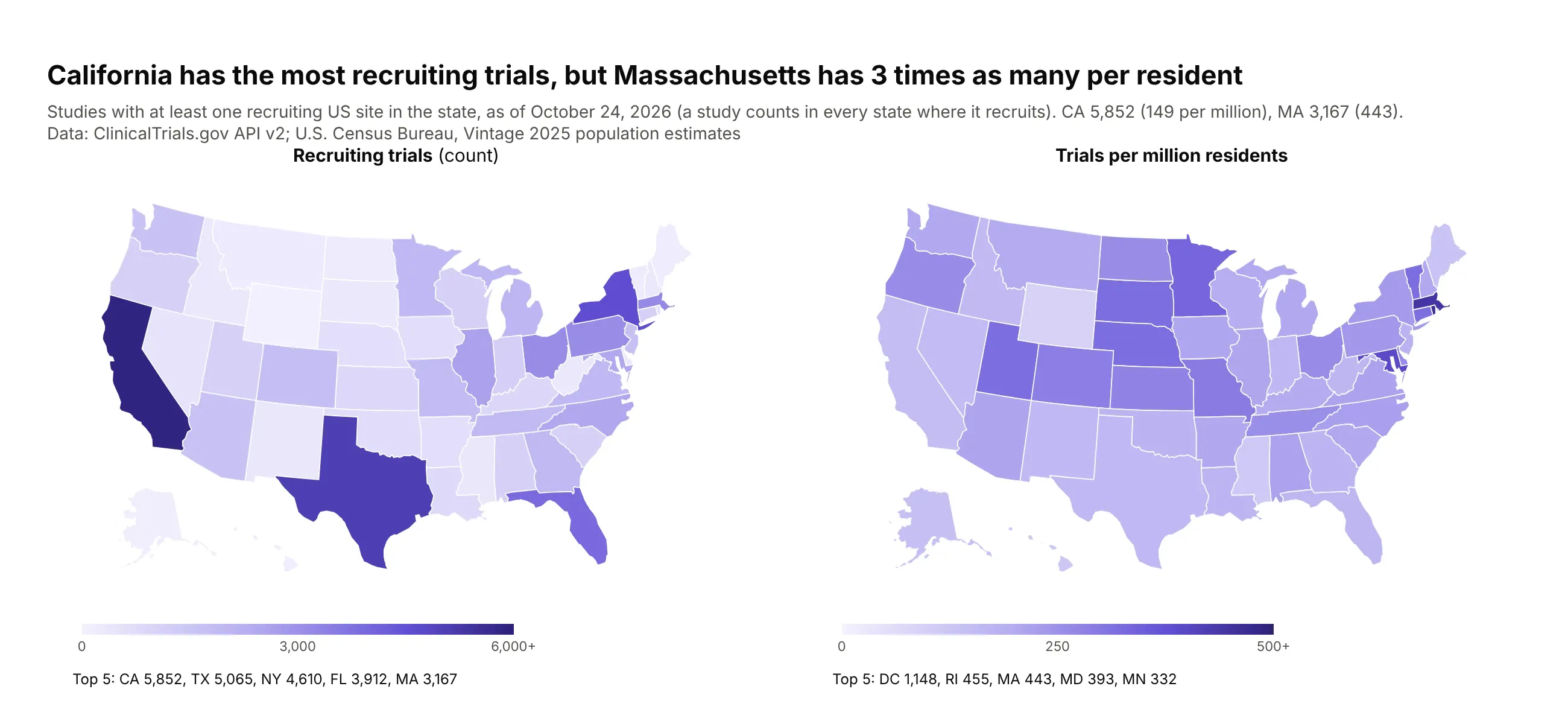
California has the most recruiting trials (5,852), but Massachusetts has three times as many per resident (443 per million against 149). The count map shows where the research centers are, and the rate map shows where a patient is most likely to find a trial. Data: ClinicalTrials.gov API v2 (October 24, 2026) and Census population.
Tip: when both questions matter, show both maps side by side, each with its own color scale.
Get the data from the ClinicalTrials.gov API v2 (one count query per state for studies with a recruiting US sitethere) and Census Vintage 2025 state population, and shape it into a table(columns: state_po, state, trials, pop_2025, per_million).Build two plotly state choropleths side by side with make_subplots: trials (capped at 6,000) andper_million (capped at 500), one purple scale each with its own colorbar, top five of each listed below.
9. Measles vaccine coverage around the world
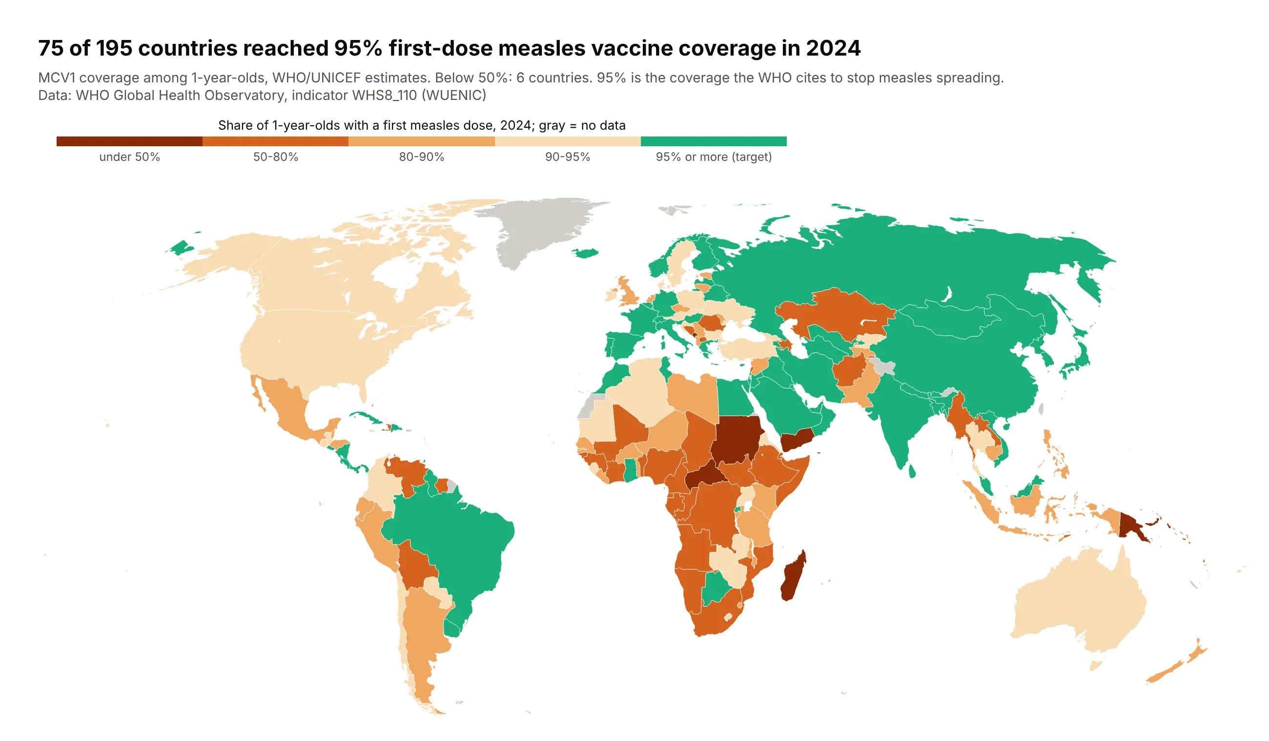
75 of 195 countries reached 95% first-dose measles coverage in 2024, the level the WHO cites to stop measles spreading, and six were below 50%. Data: WHO Global Health Observatory (WHO/UNICEF estimates).
Tip: color the target class in a different hue (green) and step the classes below it in one hue, so "on target" and "how far off" read separately.
Get the data from the WHO Global Health Observatory API (indicator WHS8_110, MCV1 coverage among 1-year-olds,2024) and shape it into a table (columns: iso3, region, mcv1_pct).Build a plotly world choropleth (Robinson) with classes under 50, 50-80, 80-90, 90-95 in orange to darkbrown and 95%+ in green, gray for no data. Title: how many countries reached 95%.
10. The 2024 election, faded by voter density
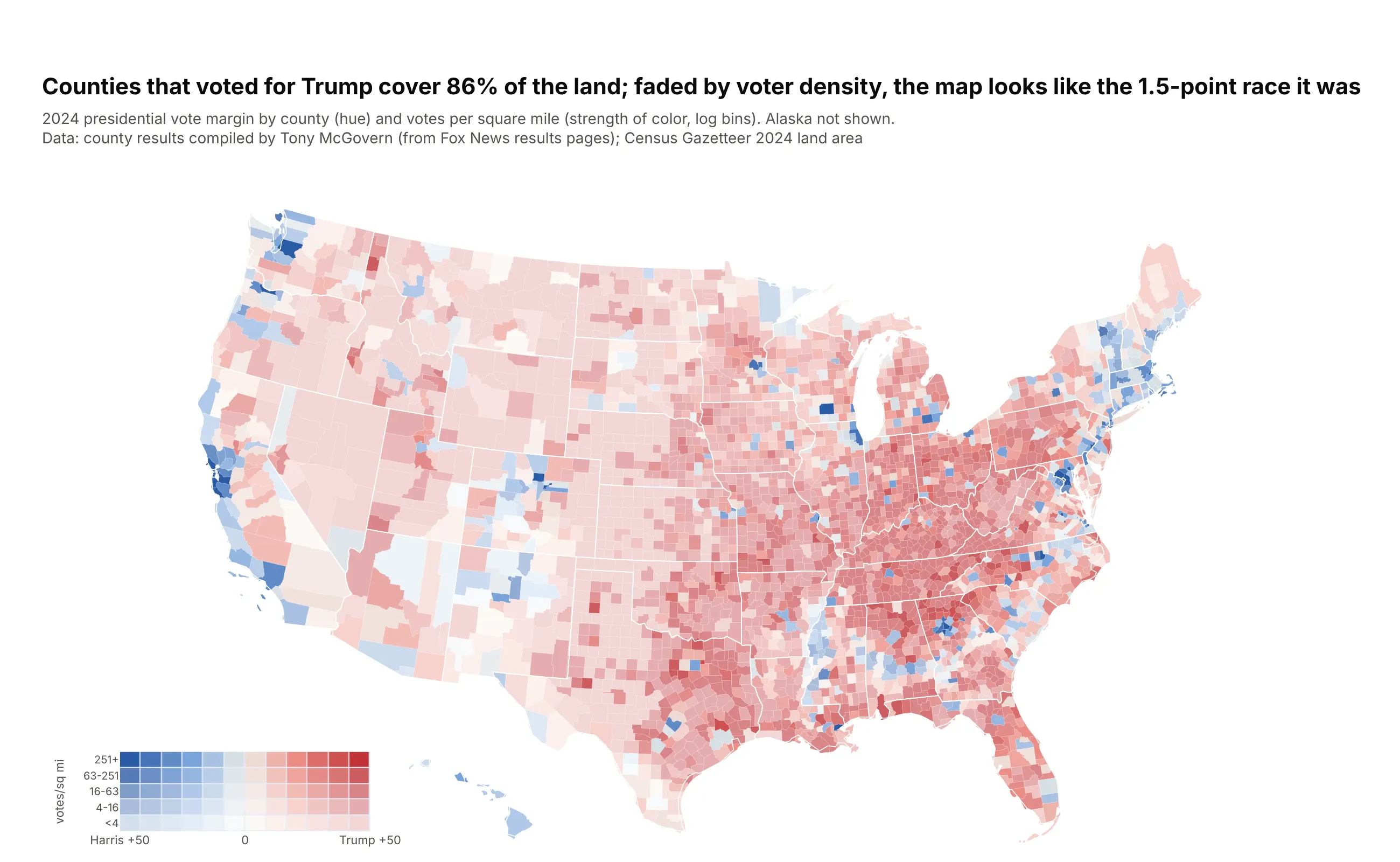
Counties won by Trump cover 86% of the land, but the popular vote margin was 1.5 points. Fading each county by votes per square mile (a value-by-alpha map, Roth, Woodruff and Johnson, 2010) lets dense counties count visually. Data: county results compiled by Tony McGovern; Census Gazetteer land area.
Tip: Plotly applies one opacity to a whole choropleth trace, so bake the fade into the colors: 12 margin bins times 5 density bins, a stepped colorscale and a small heatmap as the two-way legend.
Get the data from Tony McGovern's US_County_Level_Election_Results_08-24 (GitHub, 2024 file) and the CensusGazetteer 2024 counties file, and shape them into a table(columns: fips, state, county, votes_trump, votes_harris, votes_total, margin_pts, land_sqmi, votes_per_sqmi).Build a value-by-alpha county choropleth: hue = margin (blue-white-red), strength = log10 votes per sq miin 5 bins, mixed with white. Encode the 60 combinations as one stepped colorscale and add a smallheatmap legend. Title: Trump's share of land vs the popular vote margin.