Chris Parmer

October 27, 2026

Pareto Charts - A Complete Guide

TL;DR

A Pareto chart sorts categories from largest to smallest as bars and adds a line for the cumulative share, so you can see how few categories make most of the total.
Pareto charts are also known as Pareto diagrams, and are similar to histograms and Lorenz curves.
It's the standard quality-control chart for causes of defects, and it works for any total that splits into many parts: complaints, costs, emissions, sales.
Align the two axes (0 to the total on the left, 0 to 100% on the right), fold the long tail into one "Other" bar kept last, and use a log rank axis or a Lorenz curve when there are thousands of items.
You can make a Pareto chart with Plotly from go.Bar and go.Scatter on a second y-axis, and any coding agent can write it in a minute.

What is a Pareto chart?

Pareto charts look like this:

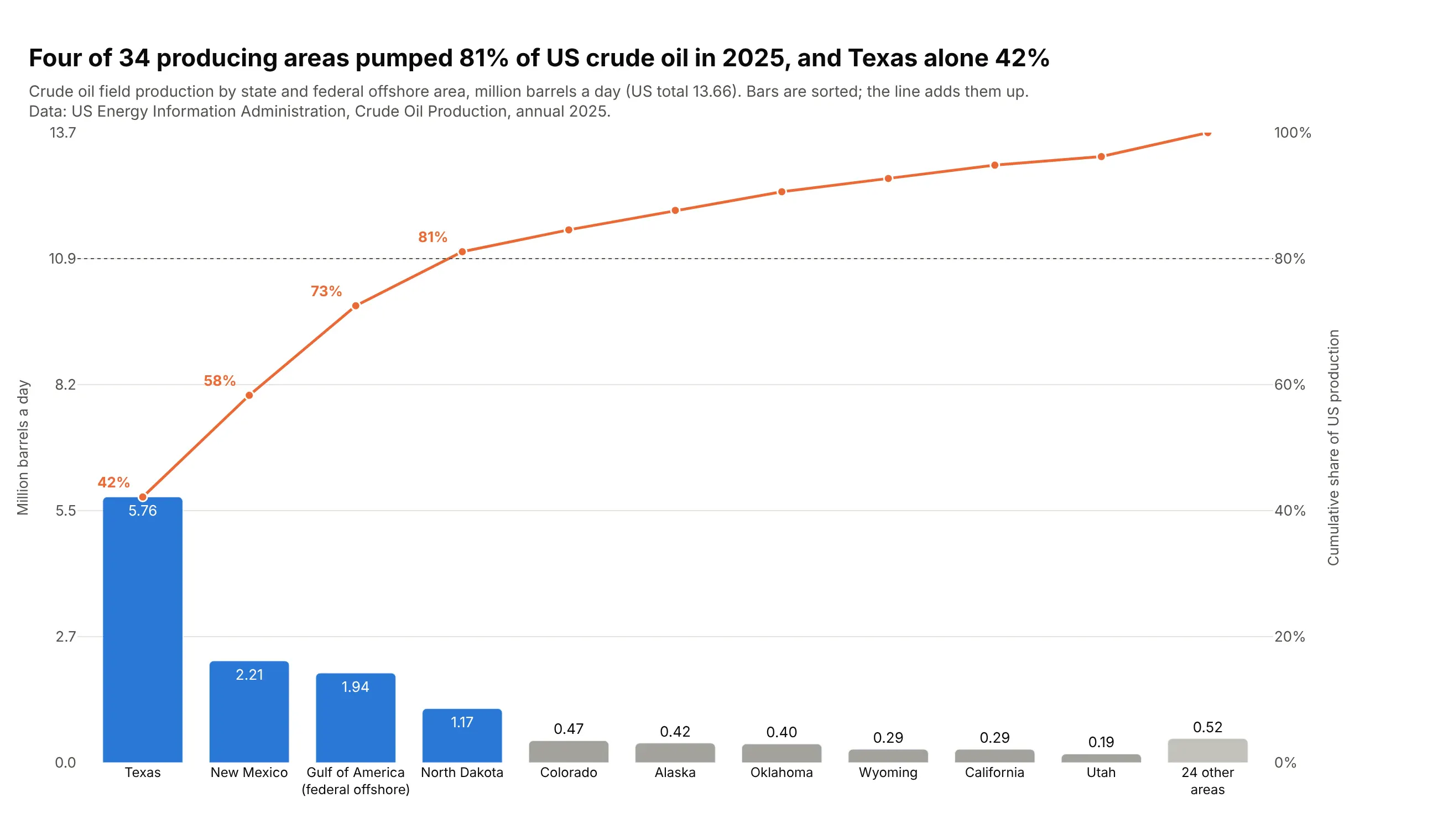
Pareto chart of US crude oil production in 2025 by state and federal offshore area. Sorted bars for Texas (5.76 million barrels a day), New Mexico (2.21), the federal offshore Gulf of America (1.94) and North Dakota (1.17) are blue, the next six states and a bar for 24 other areas are gray, and an orange cumulative line crosses the dotted 80% line at the fourth bar, at 81%

Data: US Energy Information Administration, Crude Oil Production, annual 2025.

How do you read a Pareto chart? In the example above, notice these things:

Each bar is one producing area, and its height is that area's crude oil output in million barrels a day. Texas is the tallest bar at 5.76, more than New Mexico and the federal offshore Gulf of America put together.
The bars are sorted from largest to smallest, so the few big producers sit on the left and the long tail of small ones on the right. The last bar folds 24 smaller areas into one so the tail doesn't take over the chart.
The orange line is the running total as a share of US production, read on the right axis. Each rise in the line equals the bar under it, so the line climbs steeply over Texas and New Mexico and flattens out after North Dakota.
The dotted line marks 80%, and the bars to the left of where the orange line crosses it are the few that make most of the total. Here that's the four blue bars, which together pumped 81% of US crude oil.
The two y-axes are lined up, with the left one running from 0 to the US total and the right one from 0 to 100%, which is what makes a bar and a rise in the line the same size. Check this when you read someone else's Pareto chart, because if the axes scale separately the line and the bars stop matching.

It's often used for charts like these:

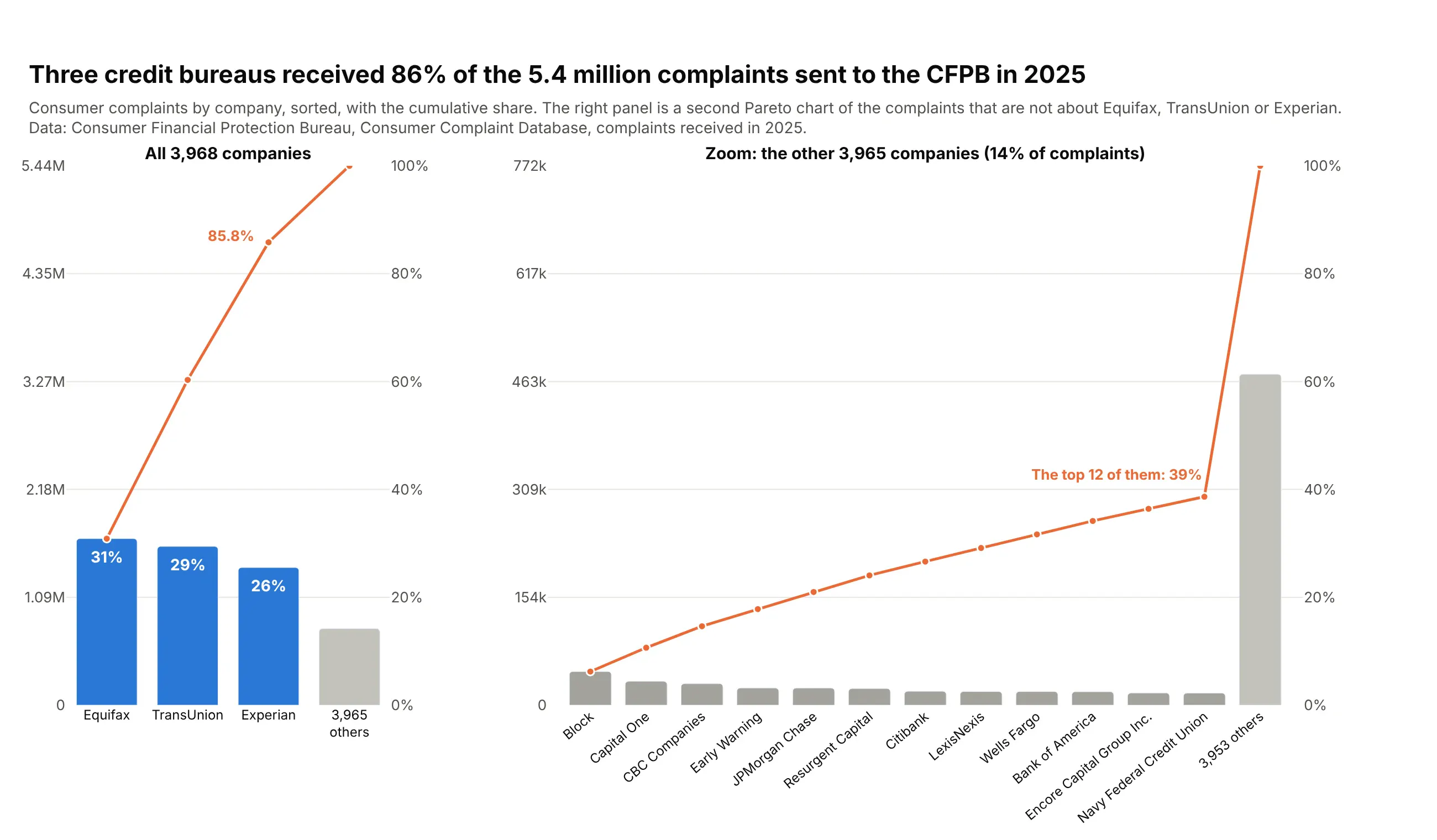
Two Pareto charts of 5.44 million consumer complaints to the CFPB in 2025. The left one has three blue bars for Equifax (31%), TransUnion (29%) and Experian (26%) and a gray bar for 3,965 other companies; the cumulative line reaches 85.8% after the three bureaus. The right one zooms into the other companies, led by Block, Capital One and CBC Companies, where the top 12 make 39% of the remainder

Complaints by company. Three credit bureaus received 86% of the 5.44 million complaints sent to the Consumer Financial Protection Bureau in 2025, and a second Pareto chart of the rest shows who comes next. Data: CFPB Consumer Complaint Database.

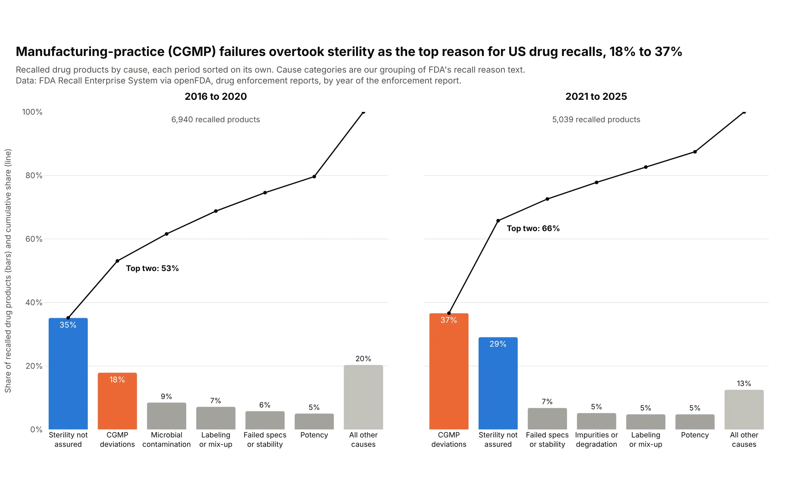
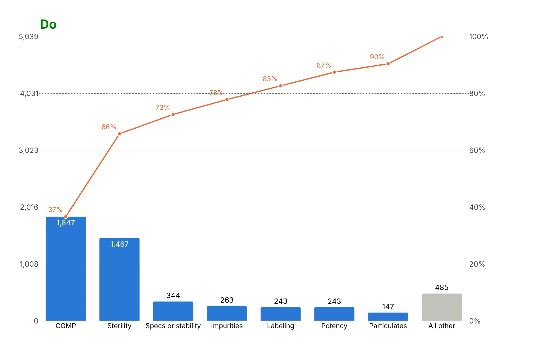
Two Pareto charts of US drug recalls by cause. In 2016 to 2020 (6,940 products), sterility not assured leads with 35% and CGMP deviations follow with 18%, top two 53%. In 2021 to 2025 (5,039 products), CGMP deviations lead with 37% and sterility follows with 29%, top two 66%

Causes of defects. This is the original quality-control use, and in US drug recalls CGMP (manufacturing practice) deviations went from 18% of recalled products in 2016-2020 to 37% in 2021-2025. Data: FDA recall enforcement reports via openFDA (cause categories are ours).

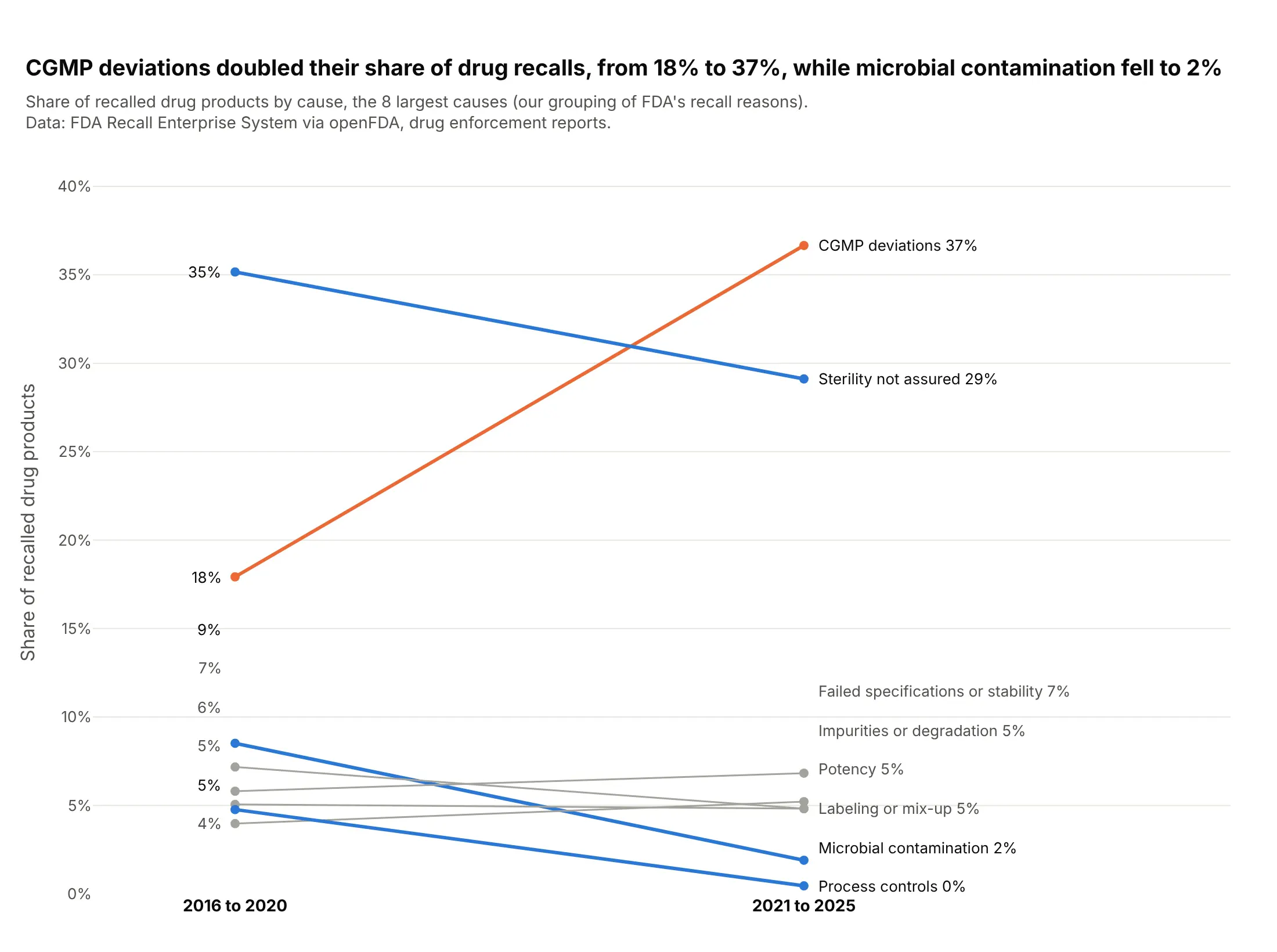
Another way to see it: a slope chart of each cause's share shows every change at once, including microbial contamination falling from 9% to 2%, which the two rankings hide.

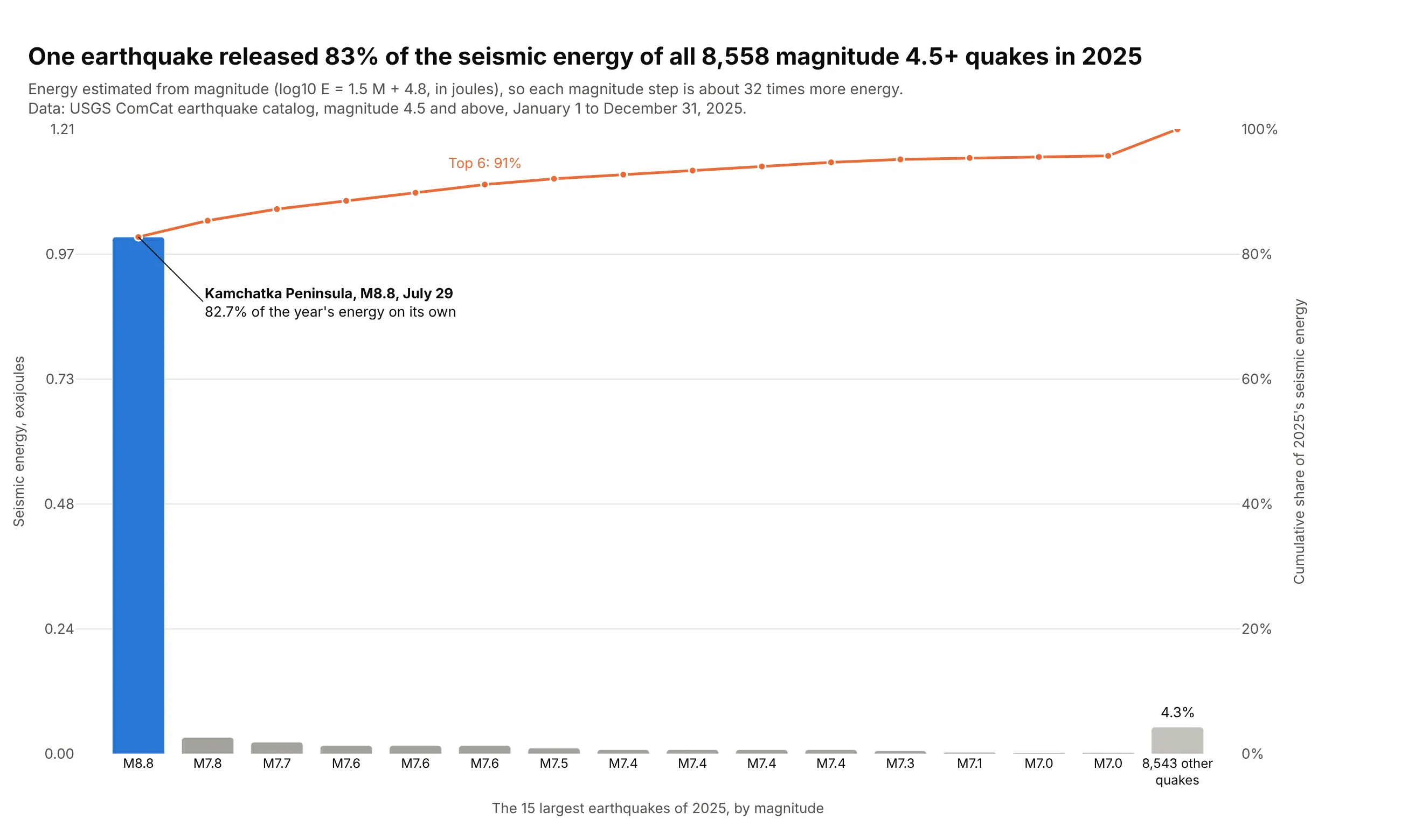
Slope chart of eight recall causes from 2016-2020 to 2021-2025. CGMP deviations rise from 18% to 37% in orange, sterility falls from 35% to 29% and microbial contamination from 9% to 2% in blue, and the other causes stay between 0% and 7%

Pareto chart of the seismic energy of the 8,558 magnitude 4.5 and larger earthquakes in 2025. One blue bar, the M8.8 Kamchatka Peninsula earthquake of July 29, reaches 82.7% of the year's energy, the next 14 quakes are thin gray bars, and a bar for the 8,543 other quakes is 4.3%

One item that dominates. The M8.8 Kamchatka earthquake released 83% of the seismic energy of all 8,558 magnitude 4.5+ earthquakes in 2025. Data: USGS earthquake catalog.

A short history

Vilfredo Pareto studied how unequally income was distributed in the 1890s, and in 1905 Max Lorenz drew the cumulative curve now named after him (Lorenz, 1905). Joseph Juran saw the same pattern in quality defects, and in the first Quality Control Handbook (1951) he put a cumulative curve of wealth next to one of quality losses and called the idea "Pareto's principle": a few causes make most of the losses. He wrote in 1974 that the name was his mistake, since Pareto never claimed the principle was universal (Juran, "The Non-Pareto Principle; Mea Culpa"). Here are the same two kinds of curves drawn with today's US data (not a redraw of Juran's figure):

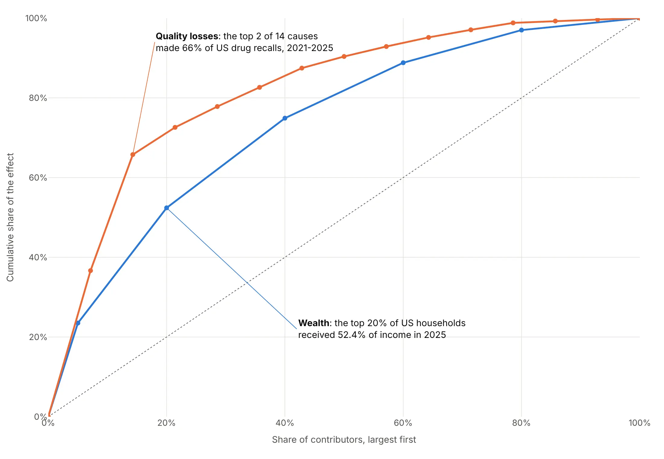
Two cumulative curves sorted largest first. Blue, wealth: the top 20% of US households received 52.4% of income in 2025. Orange, quality losses: the top 2 of 14 causes made 66% of US drug recalls from 2021 to 2025. Both curves bow far above the dotted diagonal of equal shares

The bars-plus-line chart became one of the seven basic tools of quality control, and the name stuck.

Alternatives to a Pareto chart

Here's the same oil production drawn six ways. Some are better for the question, some worse, some just different:

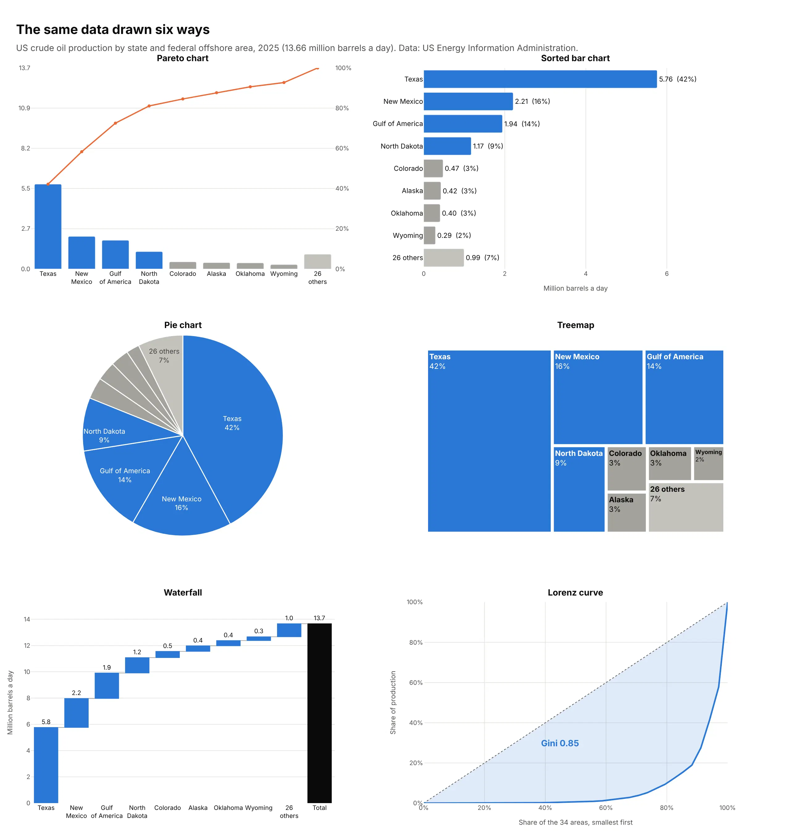
The same 2025 US crude oil production drawn six ways: a Pareto chart, a sorted horizontal bar chart with shares, a pie chart, a treemap, a waterfall that adds the states up to the 13.7 million barrel total, and a Lorenz curve with a Gini coefficient of 0.85

Sorted bar chart (works too). If nobody needs the cumulative share, sorted bars with the share printed on each are simpler and avoid the second axis.
Pie chart (worse). Fine for three or four parts, but slices past the first few are hard to compare and there is no running total.
Treemap (different). Shows part of a whole at a glance and handles a hierarchy, such as states inside regions. See our treemap guide.
Waterfall chart (different). Shows how each part builds up to the total, and handles negative parts that a Pareto chart can't. See our waterfall chart guide.
Lorenz curve (better for comparing concentration). Sorts smallest first and plots the cumulative share of the total against the cumulative share of items. The Gini coefficient, twice the area between the curve and the diagonal, puts concentration in one number (0.85 here) that you can compare across years or groups, as in examples 1, 8 and 9 below.

How to make a Pareto chart

With AI

ChatGPT, Claude Code, GitHub Copilot, Cursor and other AI tools are excellent at writing Plotly code. Name Plotly in the prompt, say what to count and how to fold the tail, and list the checks you want:

Make a plotly Pareto chart from defects.csv (columns: date, line, defect_type, units).

- Sum units by defect_type, sort largest first, keep the top 10 and fold the rest into
  one gray "All other" bar that stays last.
- Bars on the left y-axis from 0 to the total; a cumulative-share line on a second
  y-axis from 0 to 100%, with gridlines at the same heights on both.
- A dotted line at 80%; color the bars that make the first 80% and gray the rest.
- Values on the bars, the cumulative share on the line points.
- A title that states the takeaway, e.g. "3 of 24 defect types made 78% of scrap".
- Check that the line ends at exactly 100%.
- Save it as pareto.html and as a PNG at 2x scale.

With Plotly Studio

Plotly Studio is a desktop app where you point an AI at a dataset and it builds charts and a Dash app around your questions. Ask for a Pareto chart the same way:

Show a Pareto chart of complaints by product, with the cumulative share as a line, the top 10 products and the rest as "Other". Add a dropdown to switch between all complaints and complaints with a monetary loss.

Make a Pareto chart in Python or JavaScript

This is the code AI tools write under the hood. In Python, this helper sorts and folds a DataFrame and aligns the two axes. The data here is the six largest causes of US drug recalls from 2021 to 2025:

import pandas as pd
import plotly.graph_objects as go
from plotly.subplots import make_subplots


def make_pareto(df, label, value, top_n=10, other="All other"):
    s = df.groupby(label)[value].sum().sort_values(ascending=False)
    if len(s) > top_n:
        s = pd.concat([s.head(top_n), pd.Series({other: s.iloc[top_n:].sum()})])
    total, cum = s.sum(), s.cumsum() / s.sum() * 100
    fig = make_subplots(specs=[[{"secondary_y": True}]])
    fig.add_trace(go.Bar(x=s.index, y=s.values), secondary_y=False)
    fig.add_trace(go.Scatter(x=s.index, y=cum.values, mode="lines+markers"), secondary_y=True)
    fig.add_hline(y=80, line_dash="dot", secondary_y=True)
    fig.update_yaxes(range=[0, total], secondary_y=False)
    fig.update_yaxes(range=[0, 100], ticksuffix="%", secondary_y=True)
    return fig.update_layout(showlegend=False)


recalls = pd.DataFrame({
    "cause": ["CGMP deviations", "Sterility", "Specs or stability", "Impurities", "Potency", "Labeling"],
    "products": [1847, 1467, 344, 263, 243, 243],
})
make_pareto(recalls, "cause", "products", top_n=4).show()

In JavaScript, plotly.js takes the same two traces, with the line on yaxis2 laid over the first axis:

<div id="chart"></div>
<script src="https://cdn.plot.ly/plotly-4.1.1.min.js"></script>
<script>
  const causes = ["CGMP deviations", "Sterility", "Specs or stability", "Impurities", "Potency", "Labeling"];
  const products = [1847, 1467, 344, 263, 243, 243];
  const total = products.reduce((a, b) => a + b, 0);
  let run = 0;
  const cumulative = products.map(v => (run += v) / total * 100);
  Plotly.newPlot("chart", [
    {type: "bar", x: causes, y: products},
    {type: "scatter", mode: "lines+markers", x: causes, y: cumulative, yaxis: "y2"}
  ], {
    showlegend: false,
    yaxis: {range: [0, total]},
    yaxis2: {range: [0, 100], ticksuffix: "%", overlaying: "y", side: "right", showgrid: false}
  });
</script>

Set both ranges yourself. If you let Plotly autoscale them, the right axis won't start at 0 or end at 100%, and the line no longer lines up with the bars.

Share it

Every Plotly chart has a Share chart button (the cloud icon in its toolbar) that uploads it to Plotly Cloud and gives you a link. Only you can see it until you change its visibility.

For a live app, put the chart in a Dash app and publish it with the Plotly Cloud CLI. Coding agents can run these commands for you:

pip install "dash[cloud]"
plotly user login
plotly app publish

If your data has to stay in your own cloud or data center, publish to Dash Enterprise instead.

Dos and don'ts

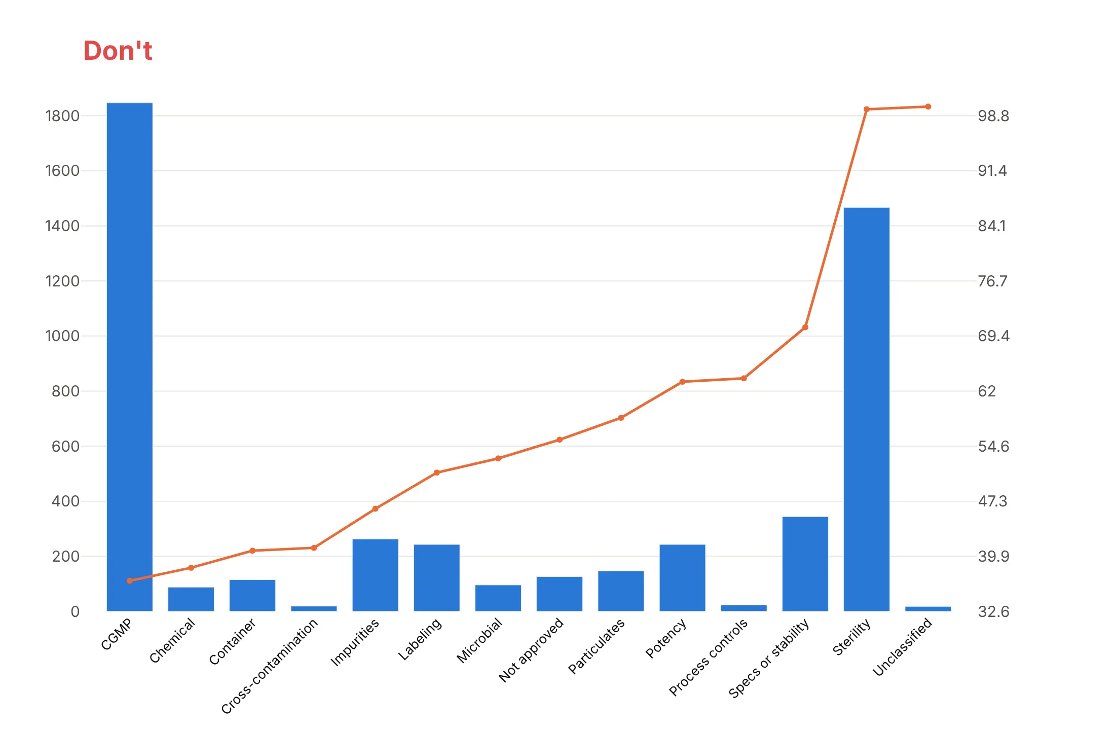
A Pareto chart only works if the bars are sorted and the two axes agree. Here is the same chart of US drug recalls by cause from 2021 to 2025 both ways, with the same colors.

Don't leave the categories in alphabetical order, draw every tiny cause as its own bar, or let the two y-axes scale themselves. Here the line's axis runs from 32.6 to about 100, so the line looks like it starts near the bottom, and the tilted labels are hard to read:

A Pareto chart of US drug recalls by cause with mistakes: 14 bars in alphabetical order from CGMP to Unclassified, so the two tall bars sit at opposite ends, tilted labels, no values on the bars, and a cumulative line on a right axis that runs from 32.6 to 98.8

Do sort largest first, fold the small causes into one "All other" bar kept last, align the axes, add an 80% line and print the values:

The same recalls as a Pareto chart done right: bars sorted from CGMP (1,847) and sterility (1,467) down to particulates (147), an "All other" bar (485) last in gray, values on the bars, the cumulative share on the line from 37% to 100%, and a dotted 80% line where the left axis reads 4,031 and the right axis 80%

Ways to show the cumulative share

The aligned two-axis chart above is the classic form. Here are three other options on the same data.

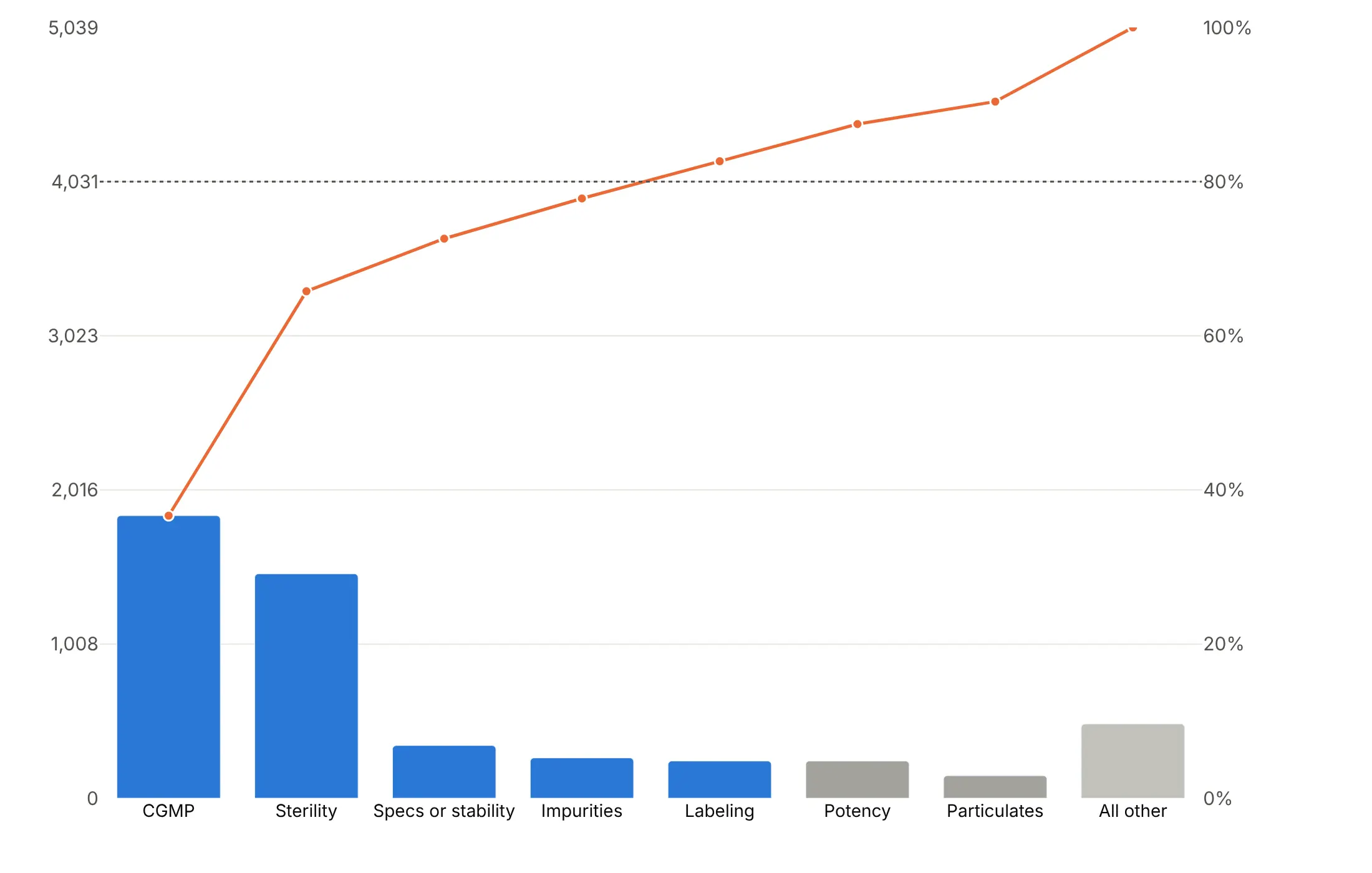
Highlight the top few. Color only the causes that make the first 80% and gray the rest, so the cut-off is visible without reading the line.

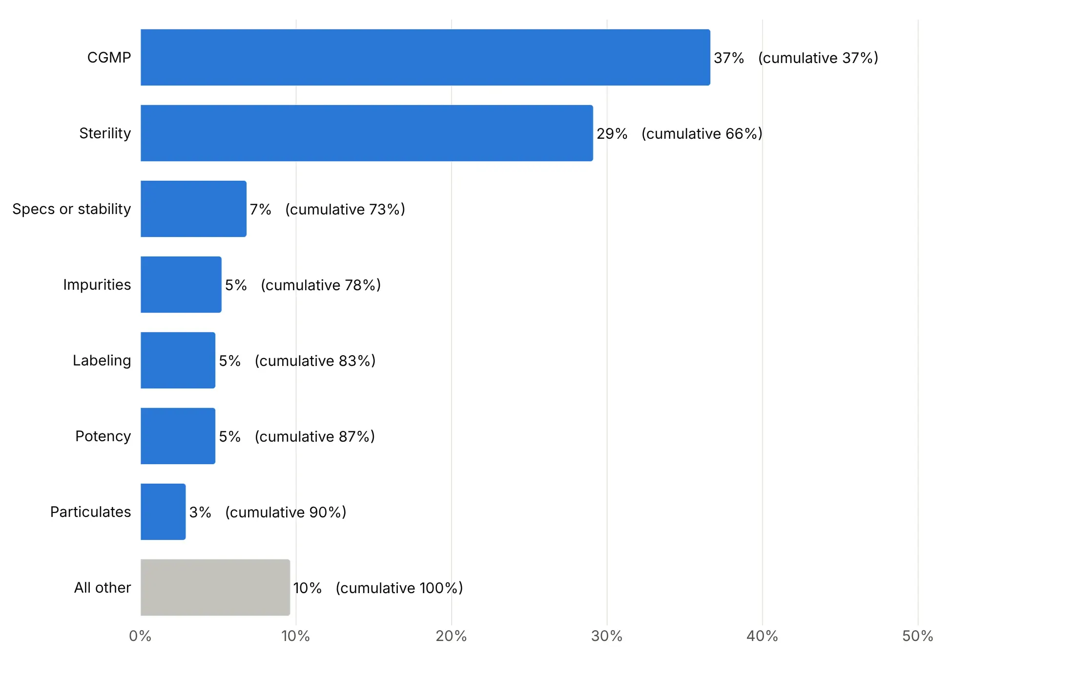
The recalls Pareto chart with the first five causes in blue, the next two and All other in gray, and a dotted line at 80%

Horizontal, with the cumulative share as text. No second axis, and long category names fit on the left.

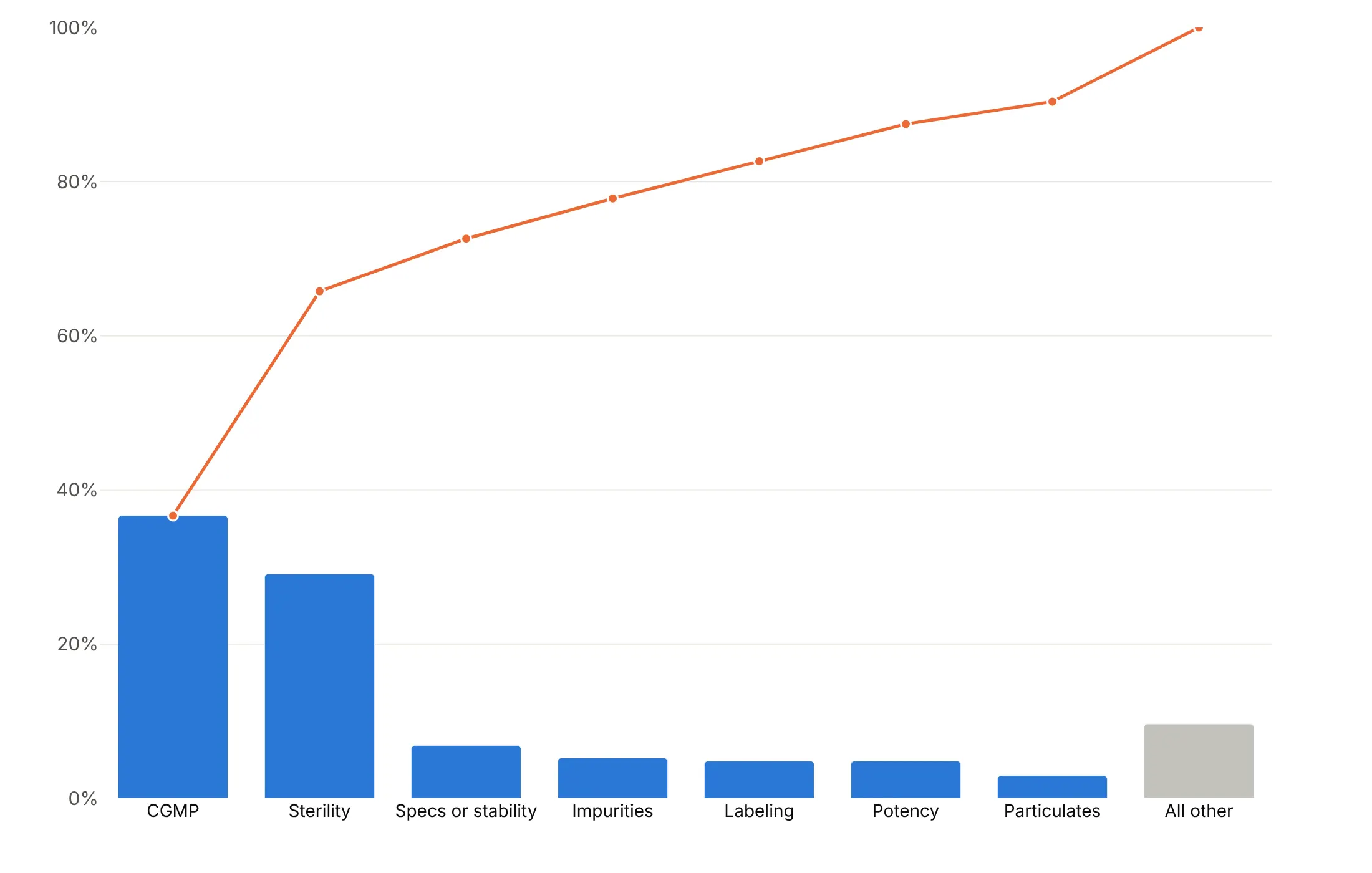
Horizontal bars of recall causes from CGMP (37%, cumulative 37%) to All other (10%, cumulative 100%), with each bar's share and the running total printed at its end

One axis. Plot the bars as shares of the total, so the bars and the line share a single 0-100% axis.

The recalls as bars of each cause's share of the total, from CGMP at 37% down, with the cumulative line on the same 0 to 100% axis

Checklist

Sort the bars largest first and keep "Other" last, whatever its size.
Set the left axis from 0 to the total and the right axis from 0 to 100%.
Write a title that says how few make how much, such as "Four of 34 areas pumped 81%".
Mark 80% (or 50%) with a dotted line, and color the bars before it.
Switch to a log rank axis or a Lorenz curve past about 50 categories.

Don't

Leave categories in alphabetical or data order.
Let the two y-axes autoscale on their own.
Show dozens of tiny bars, or tilt labels to fit them.
Add up percentages that aren't shares of one total, such as reports that list several reactions each (example 4).

Options to customize

These are the options that matter most for building a Pareto chart from go.Bar and go.Scatter. The full reference is in the Plotly bar chart and multiple axes documentation.

make_subplots(specs=[[{"secondary_y": True}]]): creates the second y-axis for the cumulative line.
fig.update_yaxes(range=..., secondary_y=...): sets each axis yourself; 0 to the total on the left and 0 to 100 on the right aligns them.
tickvals, ticktext: put gridlines at the same heights on both axes (0, 20%, 40%... of the total).
yaxis2.overlaying, yaxis2.side (plotly.js): lays the second axis over the first, on the right.
xaxis.categoryorder, categoryarray: keeps your sorted order, with "Other" last.
marker.color (a list): one color per bar, to highlight the top few or gray the "Other" bar.
text, textposition, texttemplate: values on the bars; inside for tall bars and outside for short ones.
go.Scatter(mode="lines+markers+text"): the cumulative line with its share printed at each point.
line.shape="hv": a step line, for a Pareto curve over many items (the plotly.js chart in example 2).
fig.add_hline(y=80, secondary_y=True): the 80% reference line.
orientation="h": horizontal bars for long category names.
xaxis.type="log": a log rank axis for thousands of items.
fill="tozeroy", fill="tonexty": shade the area under a cumulative or Lorenz curve.
barmode="stack": stacks each bar by sub-category (example 6).
cliponaxis=False: lets labels above the tallest bar show.
hovertemplate: shows the value and cumulative share on hover.

More Pareto chart examples

Nine more Pareto charts built from real public data, each with its source, the technique that makes it work and a prompt to rebuild it.

1. A few large facilities make most US greenhouse gas emissions

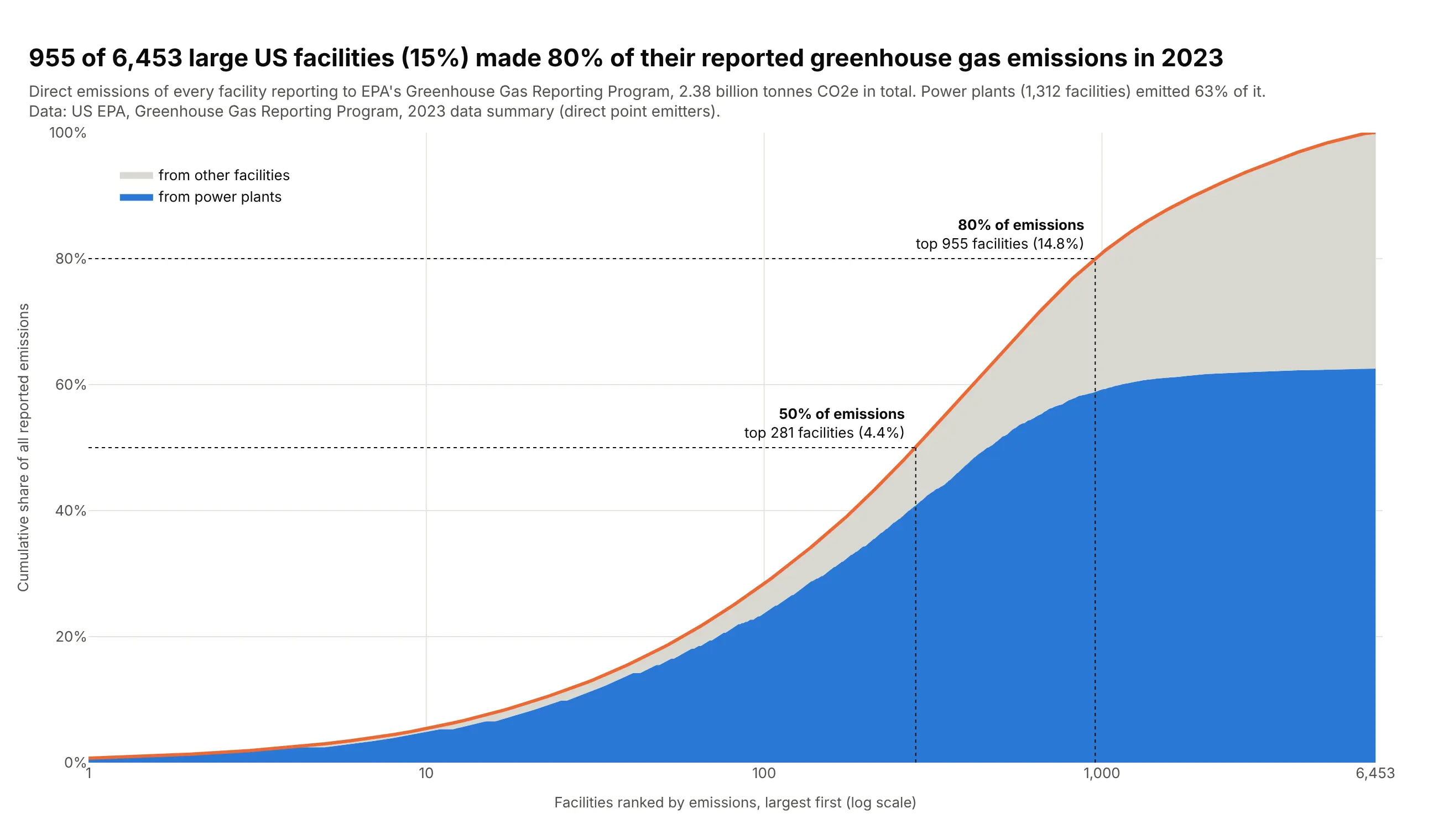
Cumulative share of 2023 greenhouse gas emissions against 6,453 large US facilities ranked on a log scale. The area under the curve is split into power plants in blue and other facilities in gray; dotted lines mark 50% of emissions at the top 281 facilities (4.4%) and 80% at the top 955 (14.8%)

Each of 6,453 facilities reporting to EPA's Greenhouse Gas Reporting Program is ranked by its 2023 emissions on a log x-axis. The top 955 (15%) emitted 80% of the 2.38 billion tonnes, and power plants made 63% of the total. Data: US EPA, Greenhouse Gas Reporting Program, 2023 data summary.

Tip: with thousands of items, drop the bars and plot only the cumulative line on xaxis.type="log", which gives the top 10 as much room as the next 90.

Get the data from EPA's Greenhouse Gas Reporting Program 2023 data summary spreadsheets
(epa.gov/ghgreporting/data-sets, ghgp_data_2023.xlsx, sheet "Direct Point Emitters")
and shape it into a table
(columns: facility_id, facility, state, sectors, tco2e = total reported direct emissions in
tonnes CO2e, power_plant = True if "Power Plants" is among the sectors).

Make a plotly Pareto curve of facility emissions.
- Sort facilities largest first; x = rank on a log axis, y = cumulative share of emissions.
- Split the area under the curve into the part from power plants (blue) and from other facilities (gray).
- Dotted guides where the curve crosses 50% and 80%, labeled with the number and share of facilities.
- Title with the 80% number; cite EPA GHGRP in the subtitle.

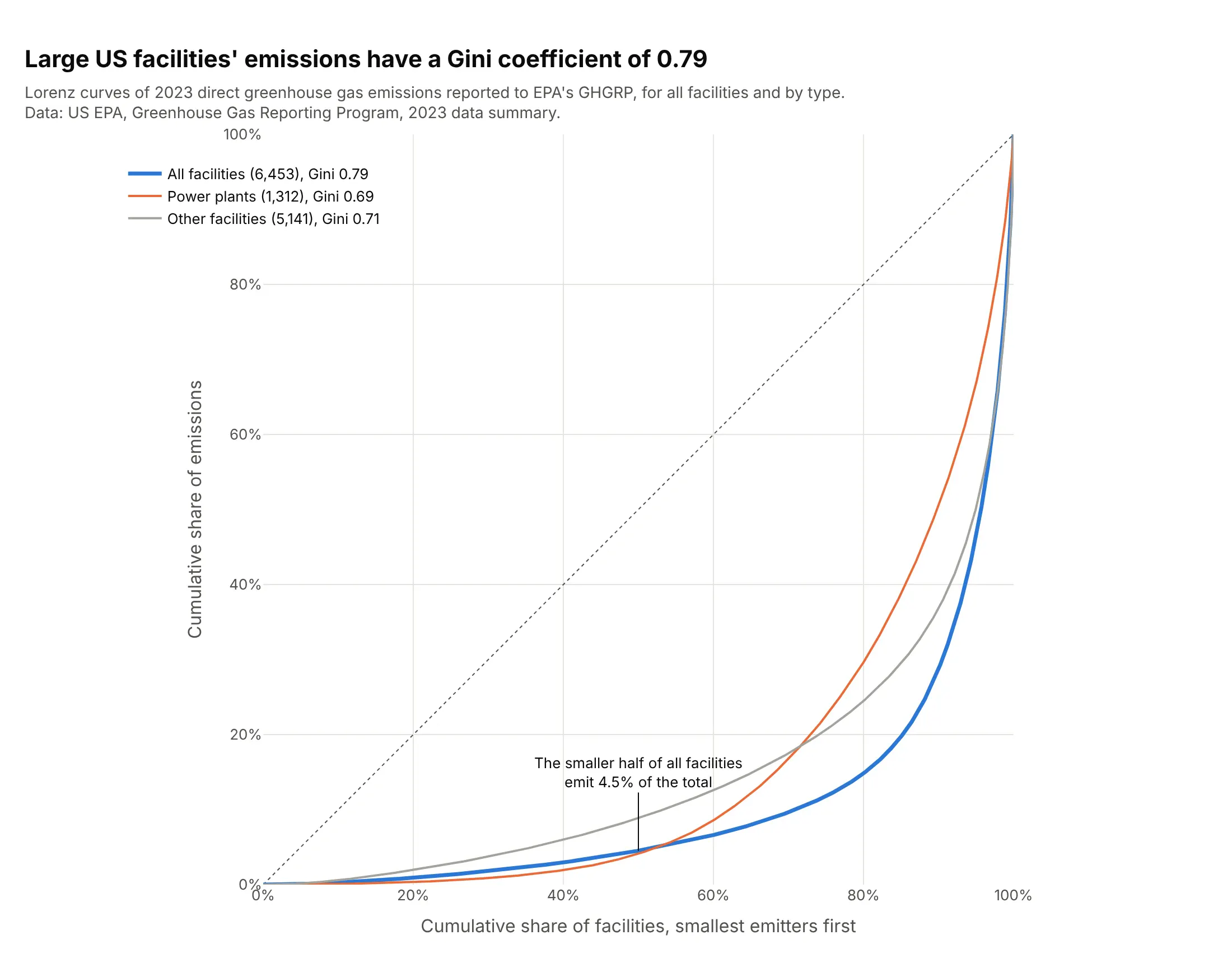
Another way to see it: a Lorenz curve of the same facilities gives a Gini coefficient of 0.79, and separate curves show that emissions are spread less unequally among power plants (0.69) than among all facilities together.

Lorenz curves of 2023 facility emissions: all 6,453 facilities with a Gini of 0.79, power plants with 0.69 and other facilities with 0.71. The smaller half of all facilities emit 4.5% of the total

2. The plotly.js commit history doesn't follow 80/20

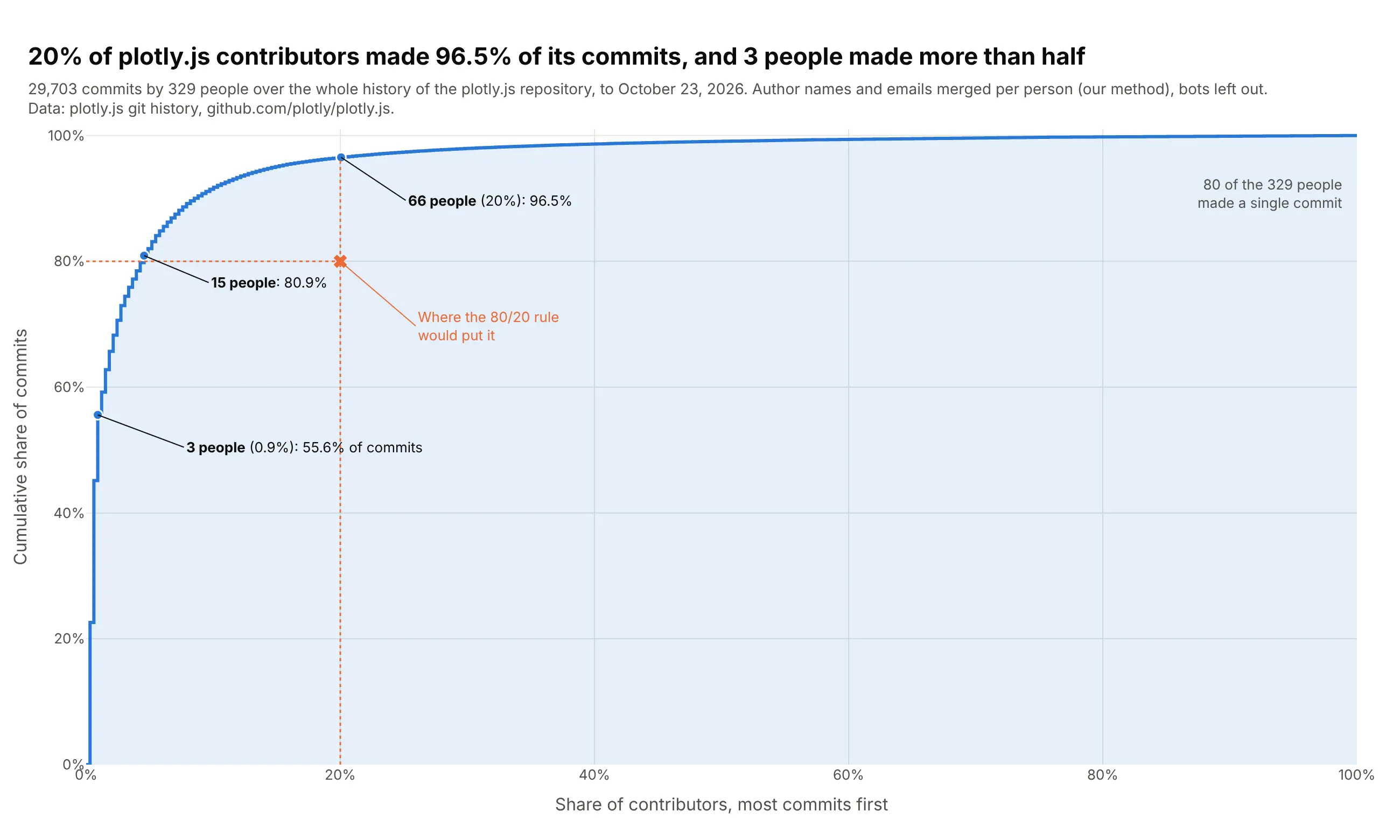
A step-shaped Pareto curve of commits to plotly.js against the share of its 329 contributors. The curve jumps to 55.6% after 3 people, reaches 80.9% after 15 people and 96.5% at 20% of contributors, far above the orange cross that marks where the 80/20 rule would put it

With the share of people on the x-axis, a Pareto curve tests the 80/20 rule directly. In the plotly.js history, 20% of its 329 contributors made 96.5% of its 29,703 commits, far more than the rule predicts. Data: plotly.js git history on GitHub.

Tip: draw the curve as a step line (line_shape="hv") over the share of contributors, and mark where the 80/20 rule would put it so readers can see the gap.

Get the data from the plotly.js git history (git clone https://github.com/plotly/plotly.js,
then git log on the default branch) and shape it into a table
(columns: author = one person after merging identities by email, name or GitHub login, commits;
leave bots out).

Make a plotly Pareto curve of commits by contributor.
- Sort people by commits, largest first; x = cumulative share of people, y = cumulative share of commits.
- A step line with a light fill under it, and a dotted guide and marker at the 80/20 point.
- Callouts for the top 3 people, the point where the curve passes 80%, and 20% of people.
- Title with the share of commits made by 20% of contributors; cite the repository in the subtitle.

3. Engines lead vehicle complaints, air bags lead crash complaints

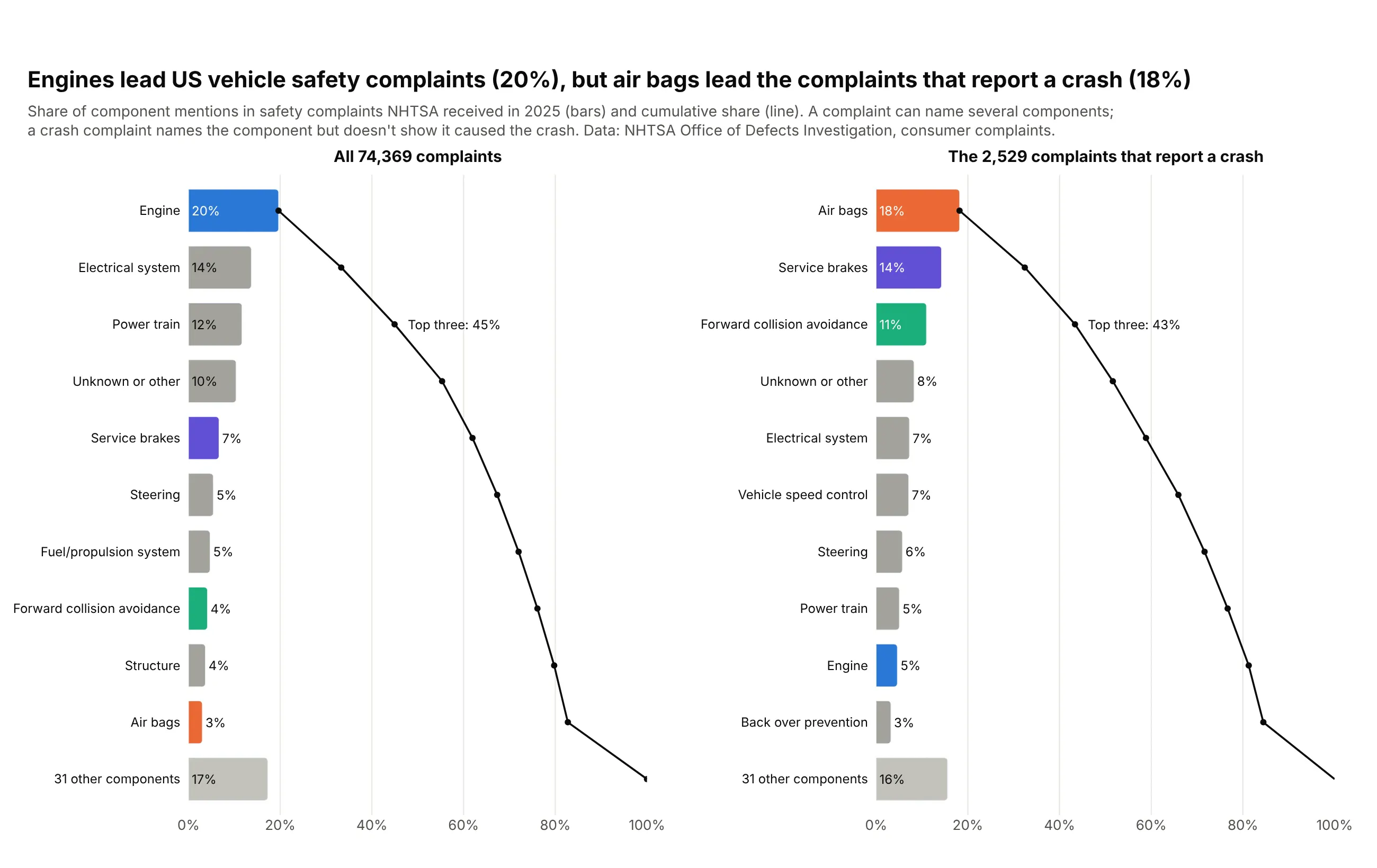
Two horizontal Pareto charts of vehicle components in safety complaints NHTSA received in 2025. By all 74,369 complaints, engine leads with 20% of component mentions and air bags are tenth with 3%. By the 2,529 complaints that report a crash, air bags lead with 18%, followed by service brakes (14%) and forward collision avoidance (11%), and engine falls to 5%

What comes first in a Pareto chart depends on what you count. By number of complaints to NHTSA in 2025, engines lead with 20% of component mentions; counting only the 2,529 complaints that report a crash, air bags lead with 18% and engines drop to 5%. Data: NHTSA Office of Defects Investigation, consumer complaints.

Tip: give each component one color in both charts so the reader can follow it when the order changes.

Get the data from NHTSA's consumer complaints flat file (static.nhtsa.gov/odi/ffdd/cmpl,
COMPLAINTS_RECEIVED_2025-2026.zip, field list in CMPL.txt)
and shape it into a table
(columns: component = COMPDESC before ":", complaints, crash_complaints, injury_complaints,
injuries, deaths; complaints received in 2025, each complaint counted once per component).

Make two horizontal plotly Pareto charts side by side: all complaints and crash complaints.
- Bars = share of component mentions, sorted, top 10 + "N other components"; cumulative line on the same axis.
- Engine, air bags, service brakes and forward collision avoidance keep one color each in both panels.
- Say in the subtitle that a complaint can name several components.

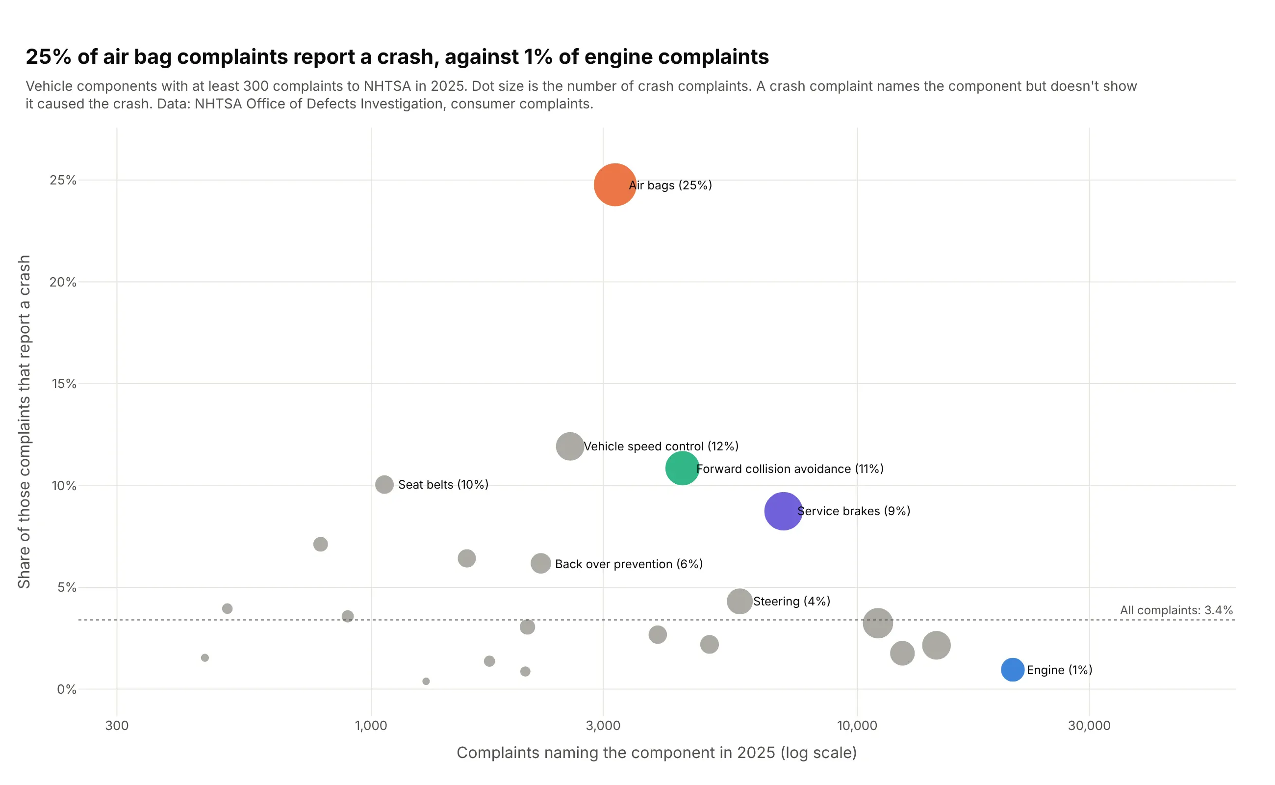
Another way to see it: a scatter of complaints against crash rate puts frequency and severity on two axes: 25% of air bag complaints report a crash, against 1% of engine complaints.

Scatter of vehicle components with at least 300 complaints in 2025, complaints on a log x-axis and the share that report a crash on the y-axis. Air bags sit highest at 25%, engine lowest at 1%, and a dotted line marks 3.4% for all complaints

4. No short list in semaglutide's adverse event reports

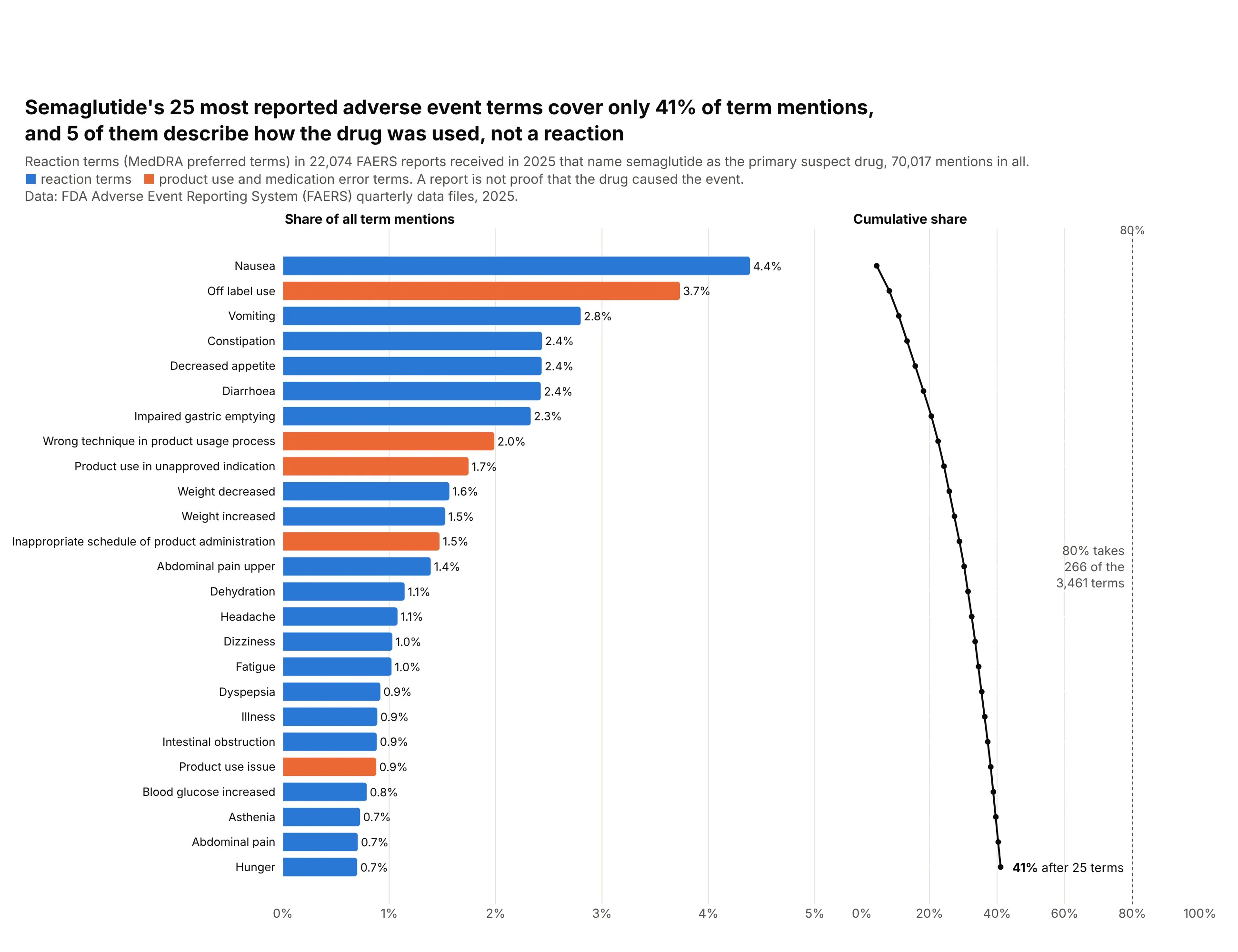
Horizontal bars of the 25 most common reaction terms in 22,074 FAERS reports on semaglutide in 2025, led by nausea (4.4%) and off label use (3.7%), with five product-use terms in orange. A separate cumulative panel reaches only 41% after 25 terms; 80% takes 266 of the 3,461 terms

A Pareto chart can also show that no short list of categories dominates. In 22,074 FDA adverse event reports on semaglutide (Ozempic, Wegovy, Rybelsus) in 2025, the top 25 of 3,461 reaction terms make only 41% of mentions, and five of them describe how the drug was used rather than a reaction. Data: FDA Adverse Event Reporting System (FAERS) quarterly data files, 2025.

Tip: each report lists about three terms, so take shares of all term mentions (which add up to 100%), not of reports.

Get the data from the FDA Adverse Event Reporting System quarterly ASCII files for 2025 Q1 to Q4
(fis.fda.gov, FAERS quarterly data extract files)
and shape it into a table
(columns: reaction = MedDRA preferred term, cases = reports naming semaglutide as primary suspect
that list the term; keep the latest version of each case and drop deleted cases).

Make a horizontal plotly Pareto chart of the 25 most common terms.
- Bars = share of all term mentions, sorted from the top; product-use and medication-error terms in orange.
- A second panel sharing the rows with the cumulative share on a 0-100% axis and a dotted 80% line.
- Note how many terms it takes to reach 80%, and that a report doesn't prove the drug caused the event.

5. 30 drugs are 46% of Medicare Part D spending

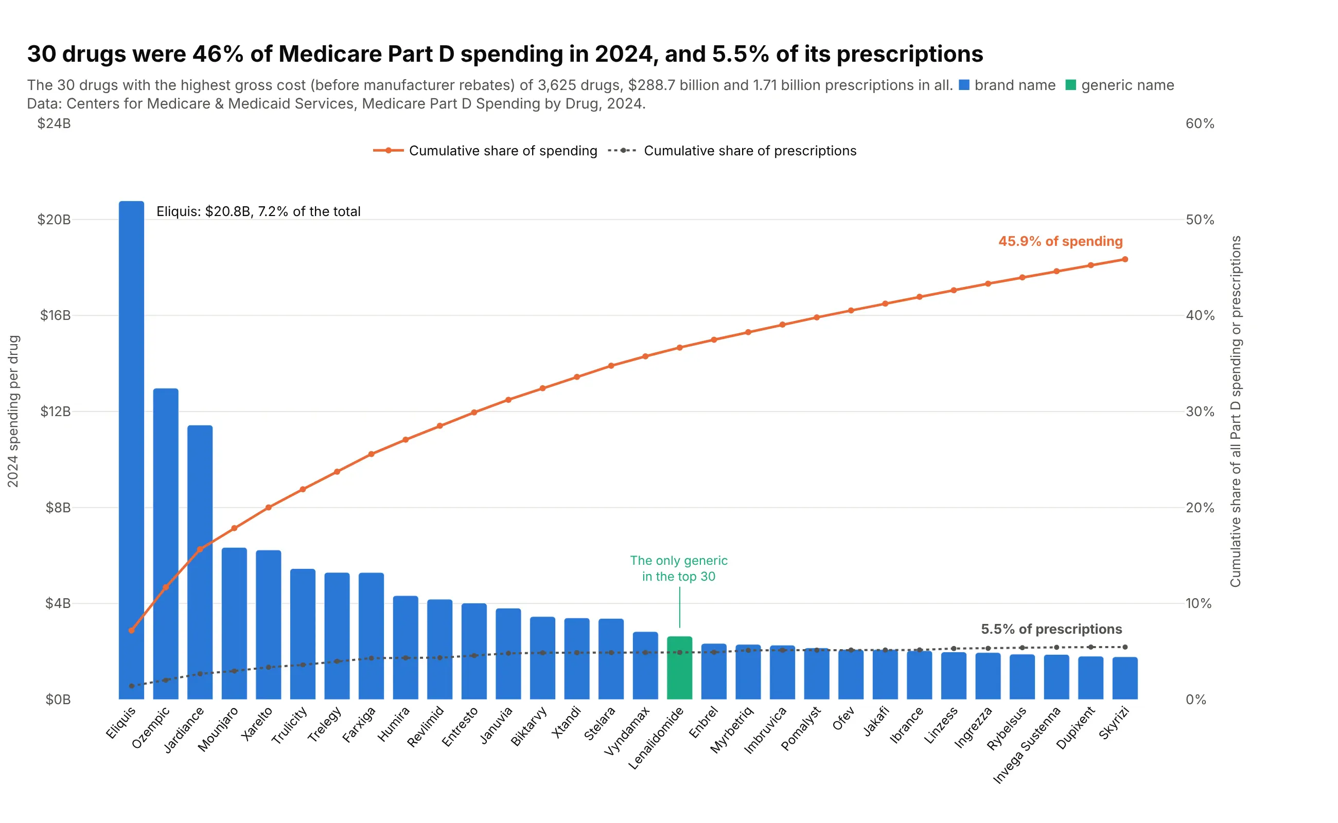
Pareto chart of the 30 drugs with the highest Medicare Part D spending in 2024, from Eliquis ($20.8B) and Ozempic ($13.0B) down to Skyrizi, with lenalidomide the only generic in green. The orange cumulative line reaches 45.9% of spending, while a dotted gray line for the same drugs' share of prescriptions reaches only 5.5%

Medicare Part D paid $288.7 billion for 3,625 drugs in 2024 before rebates. The 30 most expensive drugs were 46% of spending but only 5.5% of prescriptions, because generics fill most prescriptions for little money. Data: CMS, Medicare Part D Spending by Drug, 2024.

Tip: a second cumulative line for another measure (here prescriptions) shows when the expensive few are rarely used.

Get the data from CMS Medicare Part D Spending by Drug, 2024 (data.cms.gov)
and shape it into a table
(columns: brand, generic, spending_mn in US$ millions of gross drug cost, claims, beneficiaries,
is_generic = brand name equals generic name; one row per drug, all manufacturers).

Make a plotly Pareto chart of the 30 drugs with the highest spending.
- Bars = spending in $B, blue for brand names and green for generics, left axis from 0.
- Two cumulative lines on a right axis from 0%: share of spending (orange) and share of prescriptions (dotted gray).
- Label where each line ends; title with both numbers.

6. Memory-safety bugs lead the vulnerabilities attackers exploit

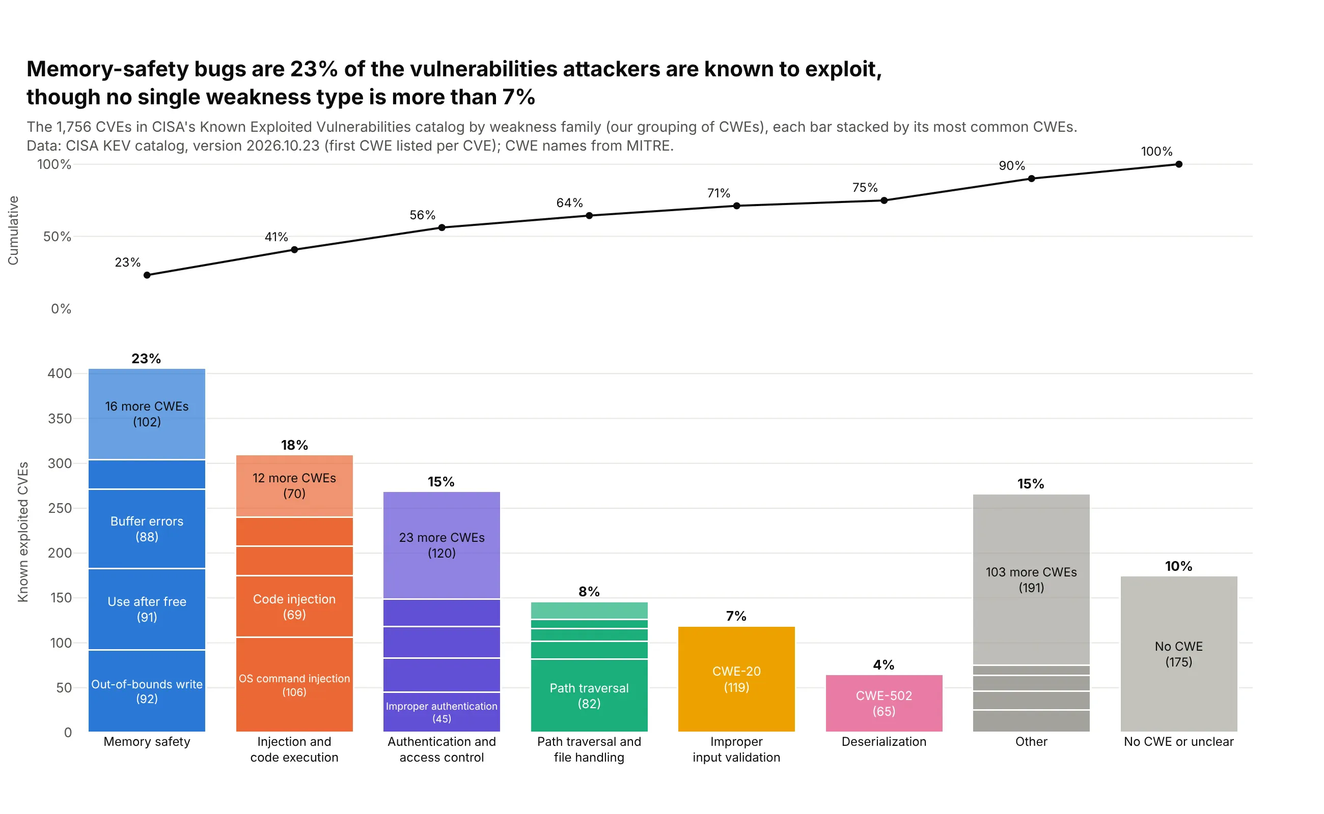
Stacked Pareto chart of the 1,756 CVEs in CISA's Known Exploited Vulnerabilities catalog by weakness family. Memory safety (23%) is stacked by out-of-bounds write, use after free and buffer errors; injection and code execution (18%) by OS command injection and code injection; authentication and access control 15%. A cumulative line in a panel above reaches 56% after three families

No single weakness type (CWE) is more than 7% of the 1,756 vulnerabilities in CISA's catalog of those known to be exploited, so a Pareto chart of CWEs is flat. Grouped into families, memory-safety bugs are 23% and the top three families 56%. Data: CISA Known Exploited Vulnerabilities catalog; CWE names from MITRE (families are our grouping).

Tip: stack each family's bar by its largest CWEs (barmode="stack") and put the cumulative line in its own panel above, so neither needs a second axis.

Get the data from CISA's Known Exploited Vulnerabilities catalog (cisa.gov, known_exploited_vulnerabilities.json)
and MITRE's CWE list (cwe.mitre.org, cwec_latest.xml.zip)
and shape it into a table
(columns: cwe, name, family = our grouping of CWEs, cves = CVEs whose first listed CWE is this one).

Make a stacked plotly Pareto chart by family.
- One bar per family, sorted, with "Other" and "No CWE or unclear" last; each bar stacked by its
  4 largest CWEs plus one segment for the rest, labeled when tall enough.
- The cumulative share in a separate panel above, sharing the x-axis.
- Title with the memory-safety share and the largest single CWE's share.

7. The Bronx's 311 requests are more concentrated than Staten Island's

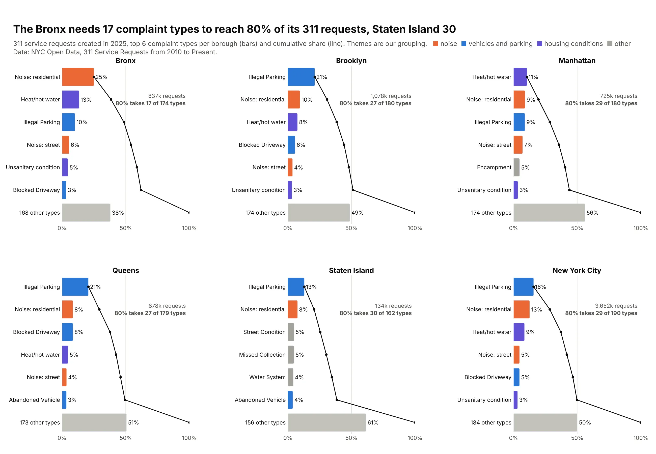
Six small horizontal Pareto charts of 2025 NYC 311 requests: Bronx, Brooklyn, Manhattan, Queens, Staten Island and the whole city. Residential noise leads the Bronx with 25%, illegal parking leads Brooklyn, Queens and Staten Island, heat and hot water leads Manhattan. Notes say 80% takes 17 of 174 types in the Bronx and 30 of 162 on Staten Island

One Pareto chart per borough shows what tops each list and how concentrated it is. The Bronx needs 17 complaint types to reach 80% of its 836,527 requests in 2025, led by residential noise (25%), while Staten Island needs 30. Data: NYC Open Data, 311 Service Requests (themes are ours).

Tip: small multiples on the same 0-100% axis let the cumulative lines be compared, and one color per theme follows noise or parking across panels.

Get the data from NYC Open Data, 311 Service Requests from 2010 to Present (data.cityofnewyork.us, erm2-nwe9)
and shape it into a table
(columns: borough, complaint_type, requests; requests created in 2025).

Make a 2x3 grid of horizontal plotly Pareto charts, one per borough plus the whole city.
- Top 6 types + "N other types" per panel, sorted; bars and cumulative line on one 0-100% axis.
- Color types by theme (noise, vehicles and parking, housing conditions, other), the same in every panel.
- In each panel, note how many types it takes to reach 80%.

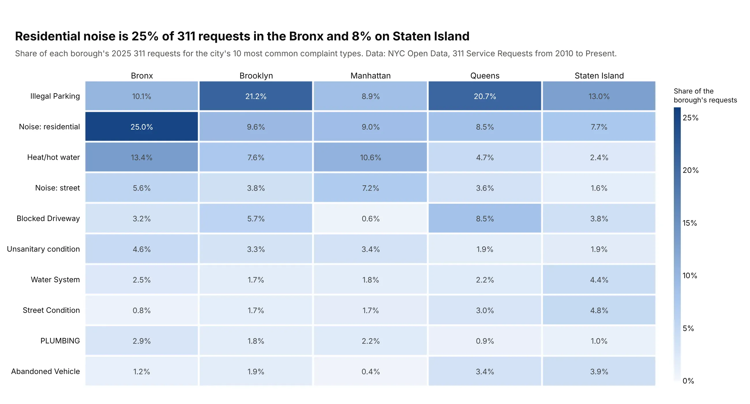
Another way to see it: a heatmap of the city's ten most common types by borough compares the boroughs type by type, with residential noise at 25% of requests in the Bronx and 8% on Staten Island.

Heatmap of the share of each borough's 2025 311 requests for the city's ten most common complaint types. Residential noise is 25.0% in the Bronx and 7.7% on Staten Island; illegal parking is 21.2% in Brooklyn and 20.7% in Queens; heat and hot water is 13.4% in the Bronx

8. The largest 10% of US banks hold 91% of deposits

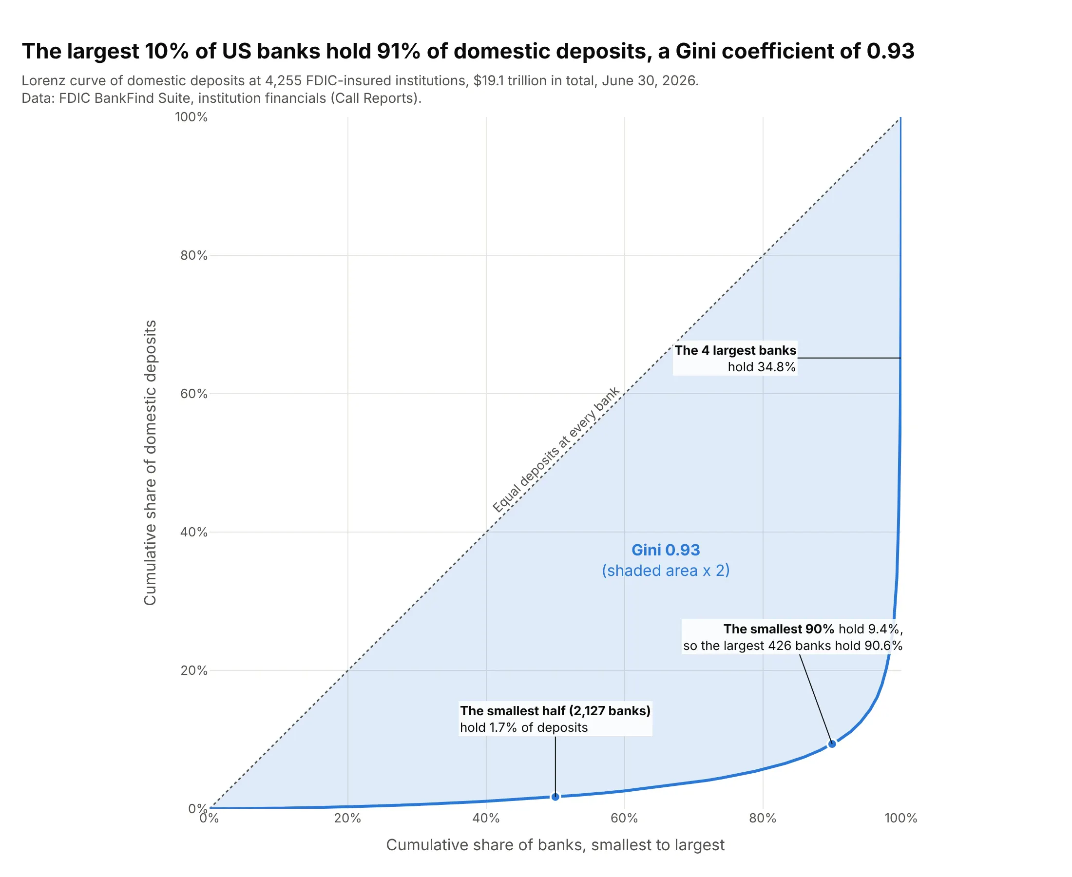
Lorenz curve of domestic deposits at 4,255 FDIC-insured institutions on June 30, 2026. The curve stays near the bottom until the right edge: the smallest half of banks hold 1.7% of deposits, the smallest 90% hold 9.4%, and the 4 largest banks hold 34.8%. The shaded area gives a Gini coefficient of 0.93

A Lorenz curve is the Pareto curve turned around, smallest first. The smallest half of 4,255 US banks hold 1.7% of the $19.1 trillion of domestic deposits, the largest 10% hold 91%, and the Gini coefficient is 0.93. Data: FDIC BankFind Suite, institution financials, June 30, 2026.

Tip: make the plot square (scaleanchor="x") so the diagonal of equal shares sits at 45 degrees, and shade the gap with fill="tonexty".

Get the data from the FDIC BankFind Suite API (api.fdic.gov/banks/financials, REPDTE 20260630)
and shape it into a table
(columns: cert, name, state, domestic_deposits_k = DEPDOM in US$ thousands; banks with deposits > 0).

Make a plotly Lorenz curve.
- Sort banks smallest first; x = cumulative share of banks, y = cumulative share of deposits.
- A dotted diagonal for equal deposits, the gap shaded, and the Gini coefficient (1 - 2 x area under the curve).
- Callouts for the smallest half, the smallest 90% and the 4 largest banks.

9. The top fifth of US households received 52% of income in 2025

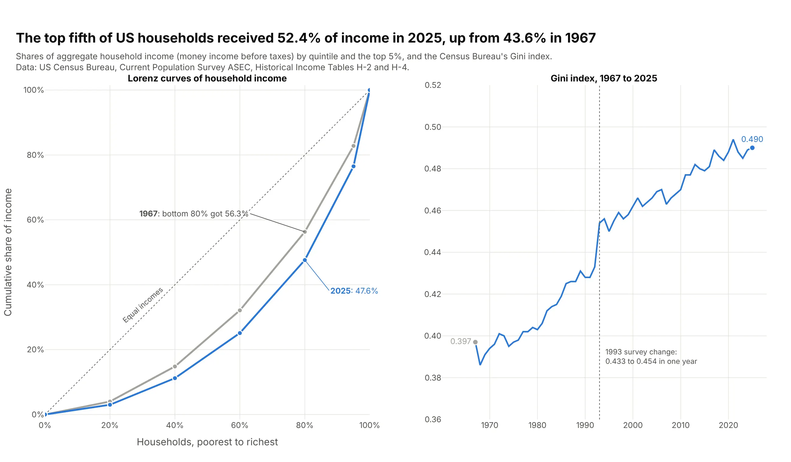
Left, Lorenz curves of US household income in 1967 (gray) and 2025 (blue): the bottom 80% of households received 56.3% of income in 1967 and 47.6% in 2025. Right, the Census Gini index rising from 0.397 in 1967 to 0.490 in 2025, with a dotted line at the 1993 survey change, when it jumped from 0.433 to 0.454

With published quintile shares instead of records, a Lorenz curve has six points, which is enough to compare years. The top fifth of US households received 52.4% of income in 2025, up from 43.6% in 1967, and the Census Gini index rose from 0.397 to 0.490, part of it from a 1993 survey change. Data: US Census Bureau, CPS ASEC, Historical Income Tables H-2 and H-4.

Tip: when the data is already grouped, plot the group boundaries as points and say so, because a curve through six points understates the true Gini.

Get the data from the Census Bureau's Historical Income Tables for households, H-2 (shares of
aggregate income by quintile and top 5%) and H-4 (Gini index) (census.gov)
and shape it into a table
(columns: year, note, households_k, q1..q5 in percent, top5 in percent, gini).

Make two plotly panels.
- Left: Lorenz curves for 1967 and 2025 through (0,0), the quintile boundaries, 95% and (100,100),
  on a square plot with a dotted diagonal; label the bottom 80% share in both years.
- Right: the Gini index for every year, with a dotted line at 1993 noting the survey change.