
Chris Parmer
November 15, 2026
Stress-Strain Curves - A Complete Guide
TL;DR
- A stress-strain curve plots how hard a material pushes back (stress, in megapascals, MPa) against how far it has stretched (strain, in percent) during a tensile test, so one line gives its stiffness, yield strength, tensile strength and ductility.
- Stress-strain curves come from tensile tests (called tension tests in the ASTM E8 standard) and are similar to line charts and scatter plots, with landmarks marked on them: the slope of the straight start is Young's modulus, the 0.2% offset line reads the yield strength, the peak is the tensile strength and the fall after it is necking.
- Plot engineering stress for reporting, and true stress for modeling and for comparing how much a metal hardens. They agree at small strains and drift apart as the specimen thins.
- You can make a stress-strain curve with Plotly from a go.Scatter line plus a straight fit for the elastic slope and a shifted copy of it for the offset yield. A short helper is below.
What is a stress-strain curve?
Stress-strain curves look like this:
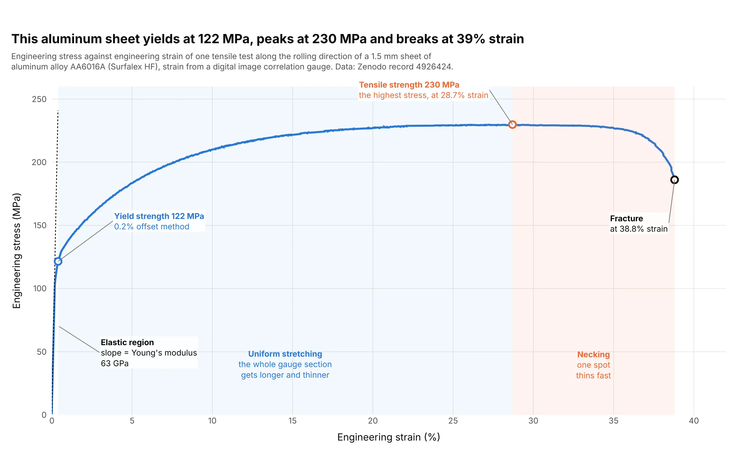
Data: Zenodo record 4926424 (CC BY 4.0), a tensile test of Surfalex HF aluminum alloy AA6016A sheet, an alloy used in car body panels, with strain measured by digital image correlation (DIC), a camera method that tracks dots on the specimen.
How do you read a stress-strain curve? In the example above, notice these things:
- The x axis is strain, the stretch as a share of the original length, and the y axis is engineering stress, the pulling force divided by the original cross-section, in megapascals (MPa, a million pascals, or newtons per square millimeter).
- The first stretch is nearly a straight line, the elastic region, where the sheet springs back if you let go. Its slope is Young's modulus, 63 GPa here (gigapascals, a thousand MPa), which tells you how stiff the material is.
- The curve bends away from that line at about 120 MPa. The 0.2% offset method puts the yield strength, where permanent stretching begins, at 122 MPa. After that the sheet keeps getting stronger as it stretches, up to a tensile strength (also called ultimate tensile strength, UTS) of 230 MPa at 28.7% strain.
- Past the peak, one spot of the sheet thins faster than the rest (necking), so the force falls, and the sheet fractures at 38.8% strain and 186 MPa. How far it stretches is a measure of ductility.
It's often used for charts like these:
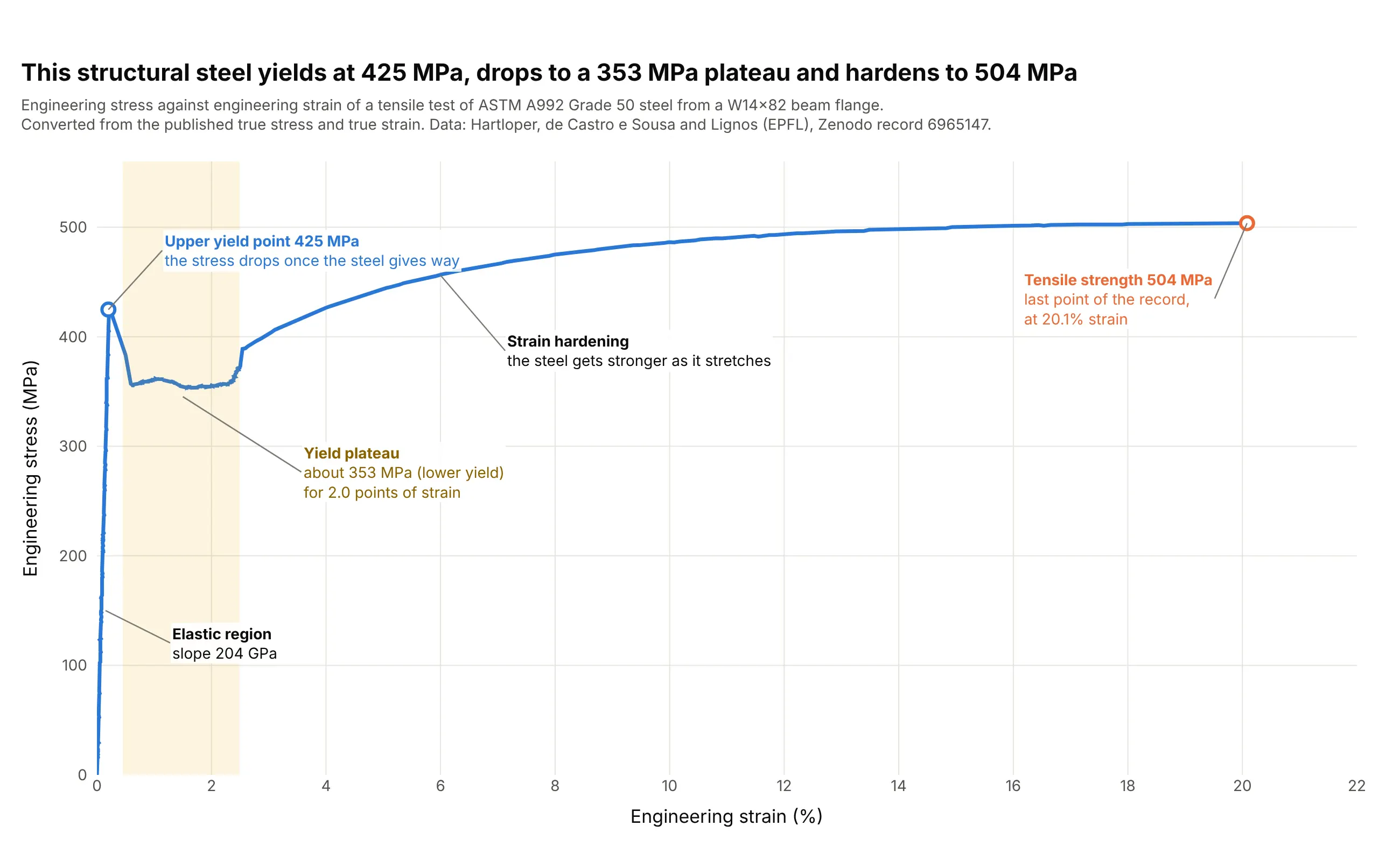
Structural engineering (the classic). Structural steel is the textbook stress-strain curve: it yields at an upper yield point of 425 MPa, drops to a plateau near 353 MPa and then hardens to 504 MPa, which is why its yield is read at the yield point and not with the offset method. Data: Hartloper, de Castro e Sousa and Lignos, database of coupon tests from the École Polytechnique Fédérale de Lausanne (EPFL), Zenodo record 6965147.
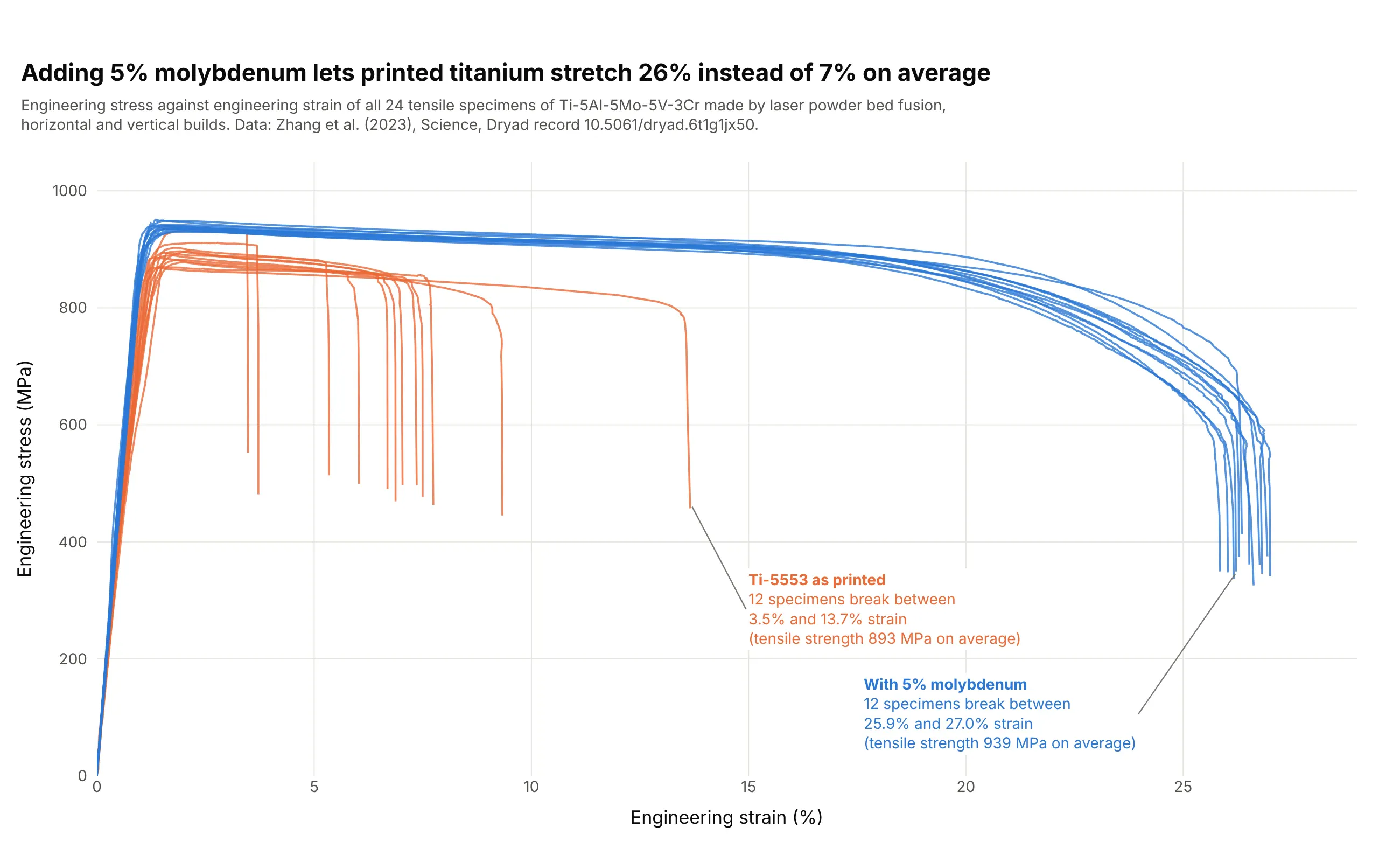
Qualifying 3D printed metal parts. Strength was almost the same with and without 5% molybdenum (893 and 939 MPa on average), but the curves show that the as-printed titanium alloy broke at 7% strain on average and the molybdenum version at 26%. Data: Zhang et al. (2023), Science, Dryad record 10.5061/dryad.6t1g1jx50.
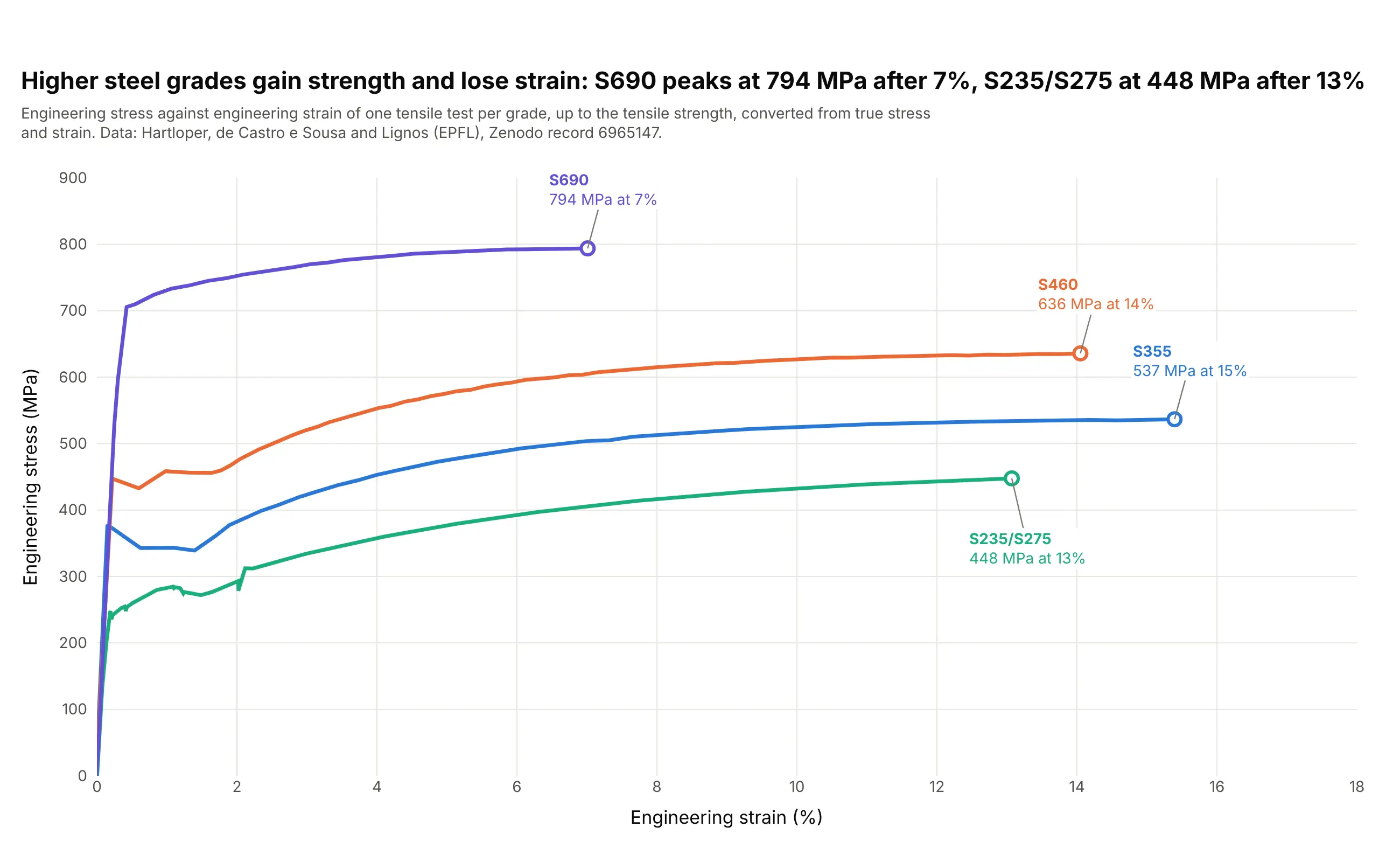
Choosing a material grade. Stacking curves shows what a stronger steel costs: the S690 plate peaks at 794 MPa after 7% strain, and the S235/S275 plate at 448 MPa after 13%. Data: Hartloper, de Castro e Sousa and Lignos (EPFL), Zenodo record 6965147.
Stress-strain curves explained
A stress-strain curve is the result of a tensile test. A specimen with a narrow middle section, the gauge section, is held in grips at both ends and pulled at a steady rate until it breaks, while a load cell records the force and an extensometer (or a camera, as with DIC) records how much the gauge section stretches. Dividing by the specimen's size turns force into stress and stretch into strain, so a thick bar and a thin sheet of the same alloy give the same curve. Test methods such as ASTM E8/E8M (from ASTM International, the standards body) and ISO 6892-1 (from the International Organization for Standardization) fix the specimen shapes and the test speed.
The two quantities are simple. Engineering stress is the force divided by the original cross-sectional area, and engineering strain is the change in length divided by the original length. A strain of 0.01, or 1%, means the gauge section is 1% longer. Each landmark on the curve answers a different design question, as described in the sections below.
The elastic region and Young's modulus
At the start, stress is proportional to strain (Hooke's law), the material springs back completely when unloaded and the slope is Young's modulus. A steeper slope means a stiffer material: the steel curve above rises at 204 GPa and the aluminum sheet at 63 GPa. In practice you fit a straight line through the rising points between two stress values, because the first points often show slack in the grips (a "toe") and the last ones start to bend:
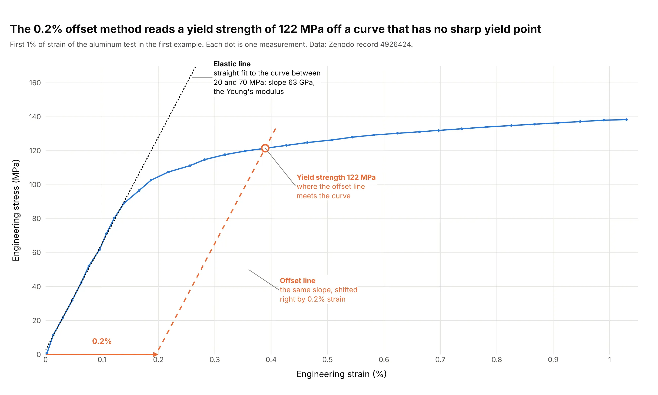
Data: Zenodo record 4926424, the aluminum test from the first example, strain from DIC. A strain gauge or extensometer clipped to the specimen usually gives a more accurate slope than a camera or the crosshead's motion.
Yield strength and the 0.2% offset method
Yield strength is the stress where permanent (plastic) deformation begins, and it sets the load a part can carry without bending out of shape. Engineers divide it by a safety factor to get an allowable stress (Wikipedia, Yield (engineering)). Many metals, such as aluminum and high-strength steels, bend away from the elastic line gradually and have no sharp yield point, so the standard way to read it is the offset method: draw a line parallel to the elastic line, shifted right by 0.2% strain, and take the stress where it meets the curve (written Rp0.2). In the picture above that is 122 MPa. Structural steel is the exception that has a sharp yield point, an upper yield point followed by a lower yield plateau, as in the A992 example, which is why for that steel the upper or lower yield point is read directly.
Strain hardening and the tensile strength
After yielding, most metals get stronger as they deform, which is strain hardening. While the specimen stretches uniformly, the curve keeps rising to the tensile strength, the highest stress it reached (230 MPa for the aluminum sheet). Strain hardening is often described with Hollomon's equation, stress = K times strain to the power n, where n is the strain-hardening exponent: on the aluminum test, a straight line on log-log axes between 3% and 25% true strain gives n = 0.26 and K = 425 MPa (see the alternatives section).
Necking and fracture
At the tensile strength, one section starts to thin faster than the metal hardens, so the load carried falls even though the metal at the neck is still getting stronger. The 19th-century engineer Armand Considère published the criterion in 1885: the neck forms where the slope of the true stress curve falls to equal the true stress. On this test the two meet at a true strain of 0.25, where the engineering curve peaks:
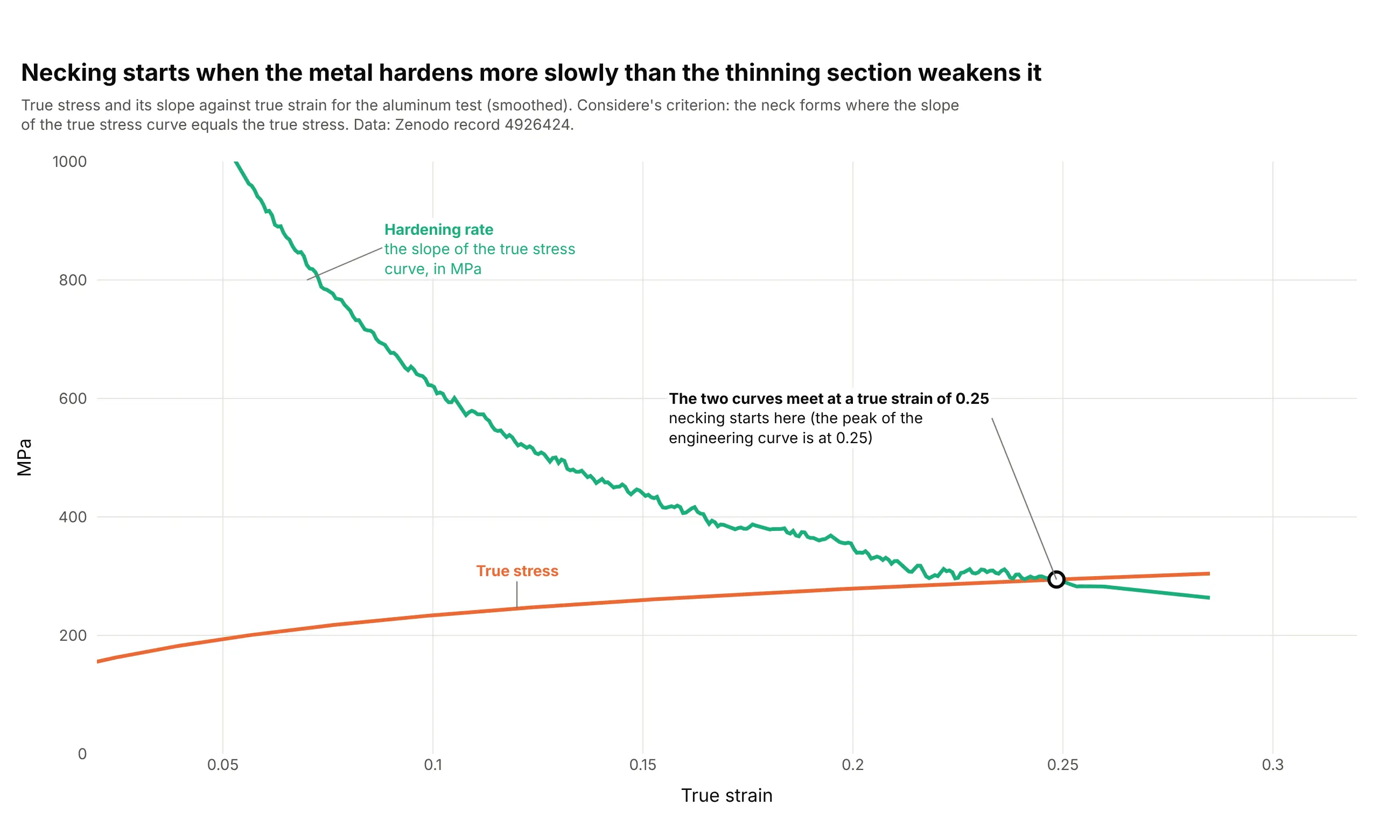
Data: Zenodo record 4926424, smoothed with a Savitzky-Golay filter (81 points, polynomial order 2) before taking the slope. The curves meet at 0.248, close to the 0.252 true strain at the engineering peak.
After the peak the specimen thins in one place until it breaks. The strain at fracture, and the percentage elongation that is measured after the two halves are put back together, are the usual measures of ductility.
Engineering stress and true stress
Engineering stress uses the original area, so after the peak it falls because the neck's area is shrinking, not because the metal weakens. True stress divides the force by the area at that moment, and while the specimen stretches uniformly it can be calculated as engineering stress times (1 plus engineering strain). The true curve keeps rising, and it is what finite element simulations need as input:
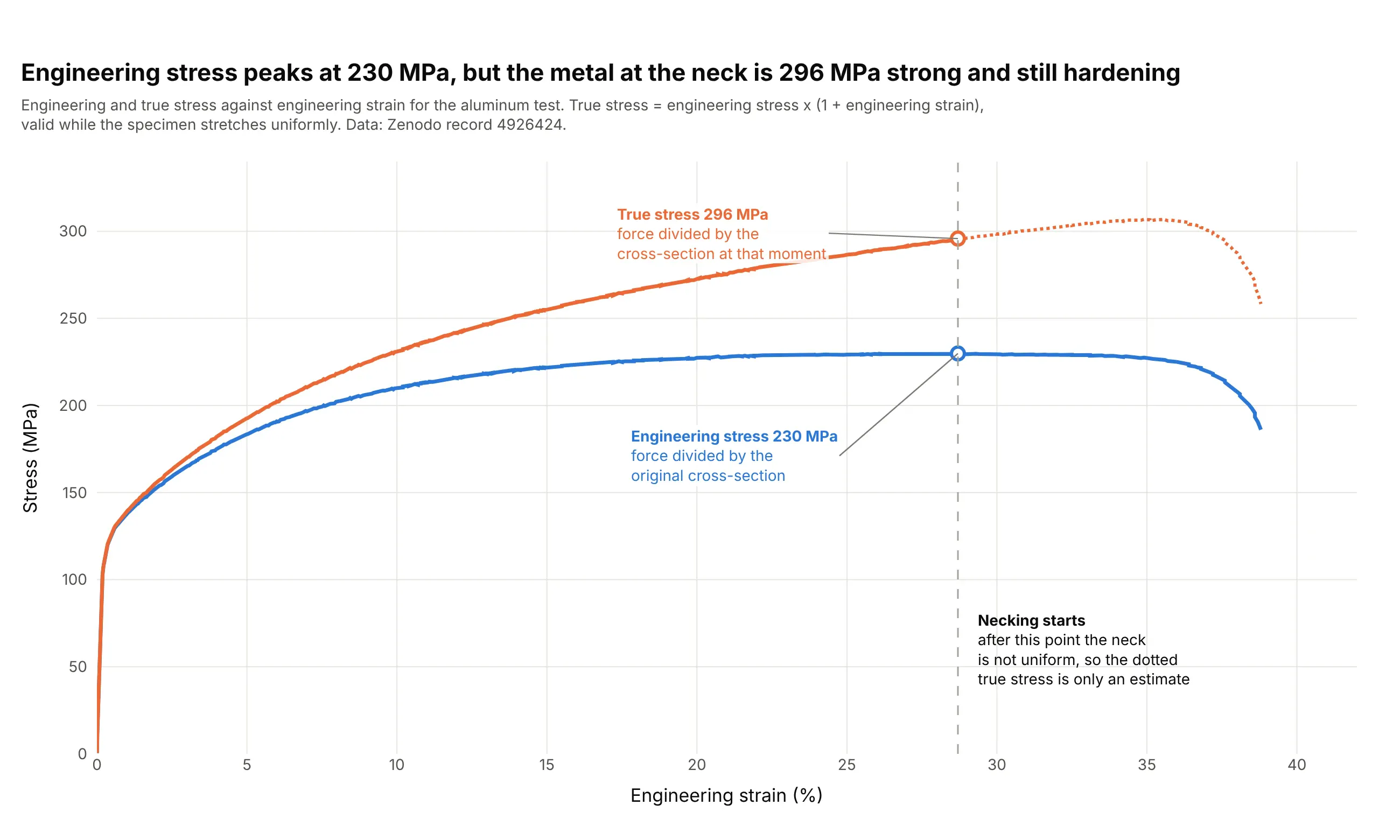
Data: Zenodo record 4926424. Beyond the dotted line the neck makes the strain uneven, so the conversion no longer describes the metal, and measuring the neck's actual diameter or area is needed.
Toughness: the area under the curve
The area under the curve is the energy per volume that the material absorbs before it breaks, called toughness. Stress in MPa times strain (a plain number) gives megajoules per cubic meter, so the aluminum sheet absorbs 82 MJ/m³, and only 0.12 MJ/m³ of it is stored elastically at the yield strength. A material with a high yield strength and a low strain at fracture can be strong but not tough:
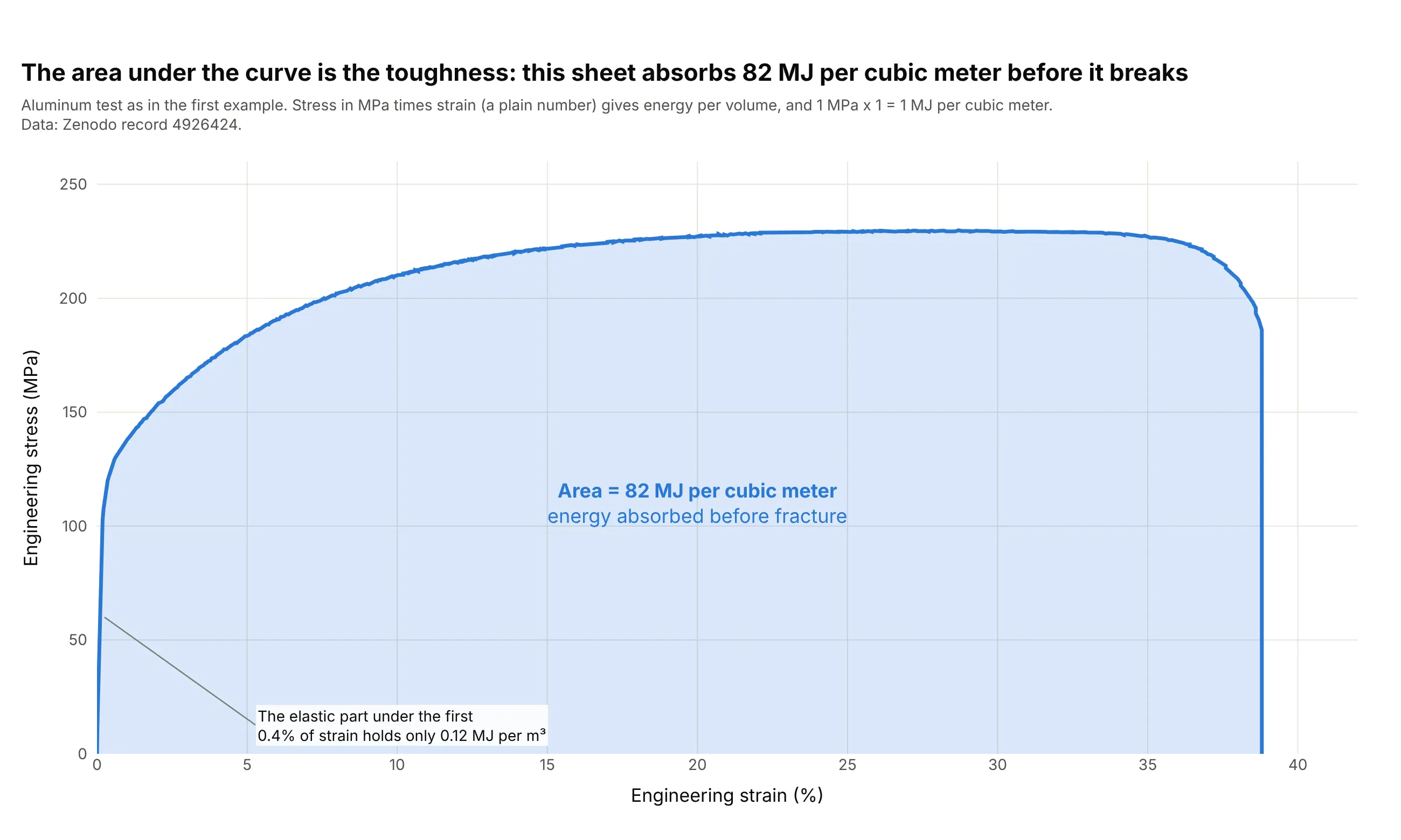
Data: Zenodo record 4926424.
What different materials look like
The shape of the curve tells you what kind of material it is. Here are six real curves, each with its own axes:
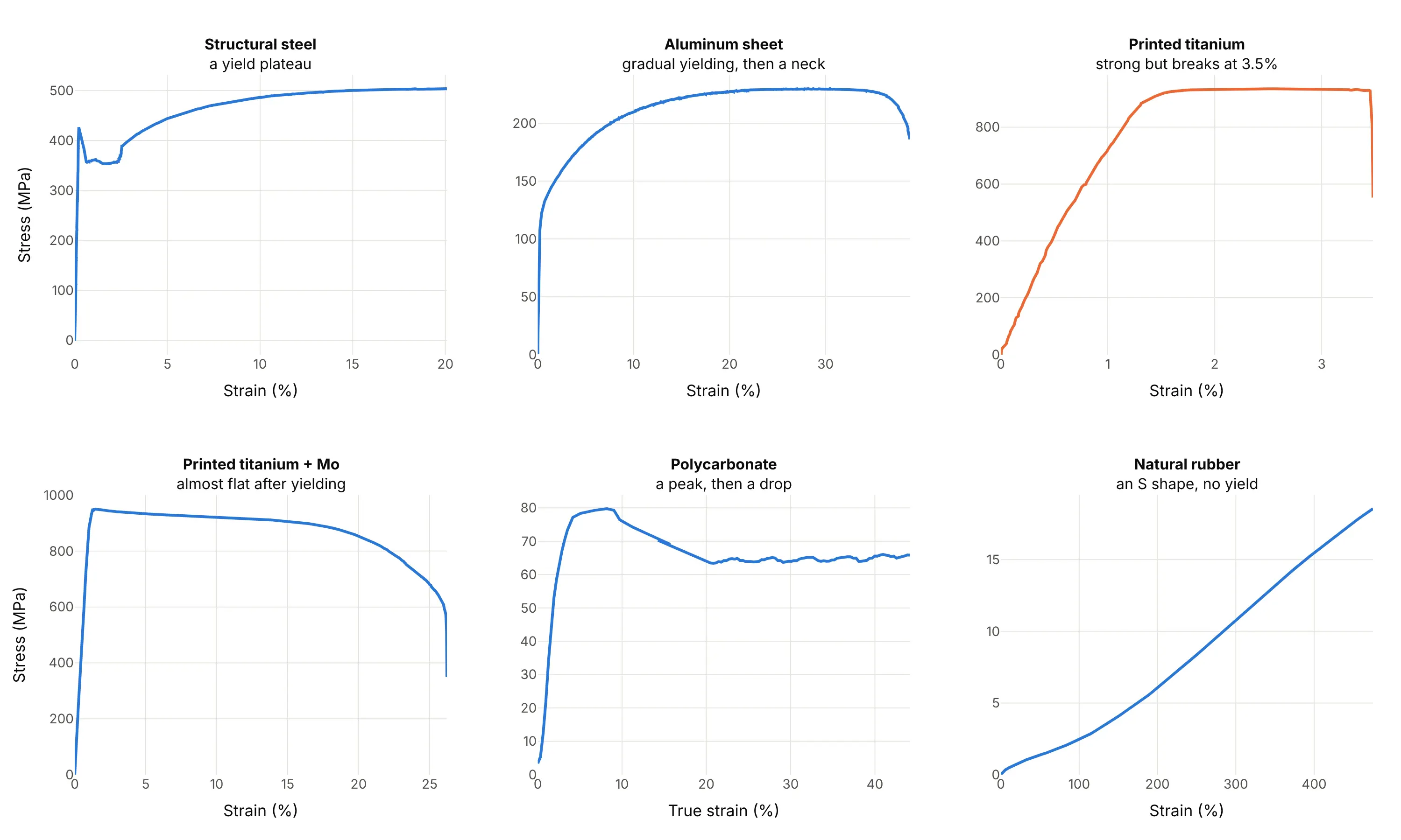
Data: the steel, aluminum, titanium, polycarbonate and rubber examples in this guide. Polycarbonate is shown as true stress against true strain, and the other curves as engineering stress and strain.
A short history
Robert Hooke stated the law that bears his name in 1676 as a Latin anagram and published the solution in 1678 as ut tensio, sic vis, "as the extension, so the force", saying he had known it since 1660 (Wikipedia, Hooke's law). The concept of Young's modulus was developed by Leonhard Euler in 1727, and Giordano Riccati did the first experiments that used it in its modern form in 1782, 25 years before Thomas Young, whose name it carries (Wikipedia, Young's modulus). Armand Considère published the necking criterion in 1885 while studying the stability of bridges (Wikipedia, Necking). The 0.2% offset convention for Rp0.2 and the specimen shapes are now set by standards such as ASTM E8/E8M and ISO 6892-1 (Wikipedia, Tensile testing). We couldn't find the data behind the early stress-strain diagrams in a public form to redraw them, so the examples here use recent open test data instead.
Alternatives to a stress-strain curve
Here's the same aluminum test drawn six ways. Some are better for the question, some worse, some just different:
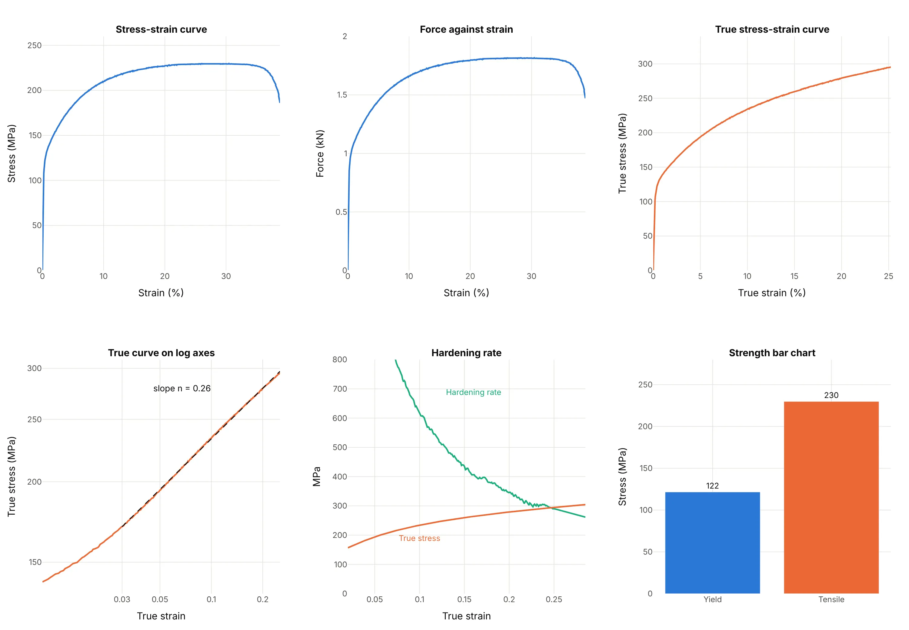
- Force against elongation (worse for comparing materials). The curve has the same shape, but the y axis is a force in kilonewtons that depends on the specimen's cross-section, so a thicker bar of the same alloy gives a taller curve. It is the raw output of the test machine, so it is the right chart for checking a test or a machine.
- True stress-strain curve (better for modeling). It keeps rising where the engineering curve peaks and gives the hardening behavior a simulation needs, but it is only valid until necking starts.
- Log-log true curve (better for fitting). The hardening part of many metals is a straight line on log-log axes, and its slope is the exponent n of Hollomon's equation (0.26 here), which is a single number to compare alloys with.
- Hardening rate against strain (better for finding the neck). It shows where the slope of the true curve meets the true stress, the Considère point, more precisely than reading the peak of a flat curve.
- Bar chart of strengths (different). Yield and tensile strength in one glance suit a datasheet or a ranking of many materials, as in example 9, but the bars lose the stiffness, the hardening and the ductility.
- Line chart (works too). A stress-strain curve is a line chart whose x axis is strain instead of time. Use the guide to style the line, and add the landmarks as annotations and markers.
How to make a stress-strain curve
With AI
ChatGPT, Claude Code, GitHub Copilot, Cursor and other AI tools are excellent at writing Plotly code. Name Plotly in the prompt, and say how to find the yield point:
Make a plotly stress-strain curve from tensile_test.csv (columns: strain_pct, the engineering strain inpercent, and stress_mpa, the engineering stress in MPa).- Draw the curve as a go.Scatter line, 3 px wide, with both axes starting at zero and titles"Engineering strain (%)" and "Engineering stress (MPa)".- Fit the elastic slope with np.polyfit on the rising points between 20 and 70 MPa and report Young'smodulus in GPa.- Draw the 0.2% offset line (the same slope, shifted right by 0.2% strain) and mark where it meets the curveas the yield strength.- Mark the tensile strength (the highest stress) and the last point before the load drops as fracture,with labels that state the value and the strain.- Check: print the modulus, yield strength, tensile strength and strain at fracture.
With Plotly Studio
Plotly Studio is a product for creating data visualizations and Dash apps and for analyzing data with AI, available as a desktop app or embedded in Dash apps. Ask for a stress-strain curve the same way:
Plot engineering stress against strain for every specimen in this folder of tensile tests, one color per alloy, with the 0.2% offset yield strength marked on each curve and a dropdown to switch between engineering and true stress.
Make a stress-strain curve in Python or JavaScript
This is the code AI tools write under the hood. In Python, the curve is a go.Scatter line, the elastic slope is a straight-line fit with NumPy, and the offset yield is the first point where the curve falls below the shifted line:
import numpy as npimport pandas as pdimport plotly.graph_objects as godf = pd.read_csv("tensile_test.csv") # strain_pct (%), stress_mpa (MPa)strain, stress = df.strain_pct.to_numpy(), df.stress_mpa.to_numpy()peak = stress.argmax()# Elastic slope: a straight line through the rising points between 20 and 70 MParise = (stress >= 20) & (stress <= 70) & (np.arange(len(stress)) <= peak)slope, intercept = np.polyfit(strain[rise], stress[rise], 1) # MPa per percent of strain, and MPamodulus_gpa = slope * 100 / 1000# 0.2% offset: the same line shifted right by 0.2 percentage points of strainoffset_line = slope * (strain - 0.2) + interceptabove = stress > offset_linestart = np.argmax(stress > 0.2 * stress[peak]) # skip the start, where the curve is under the line by noisecross = start + np.argmax(~above[start:])yield_strength = stress[cross]fig = go.Figure([go.Scatter(x=strain, y=stress, mode="lines", line=dict(width=3), name="Engineering stress"),go.Scatter(x=[0.2, strain[cross]], y=[intercept, yield_strength], mode="lines", line=dict(dash="dash"), name="0.2% offset"),go.Scatter(x=[strain[cross], strain[peak], strain[-1]], y=[yield_strength, stress[peak], stress[-1]], mode="markers+text",text=["Yield", "Tensile strength", "Fracture"], textposition="top right", marker=dict(size=11), showlegend=False),])fig.update_layout(xaxis_title="Engineering strain (%)", yaxis_title="Engineering stress (MPa)",xaxis_rangemode="tozero", yaxis_rangemode="tozero")fig.show()print(f"E = {modulus_gpa:.0f} GPa, yield {yield_strength:.0f} MPa, tensile strength {stress[peak]:.0f} MPa")
To get true stress and strain while the specimen stretches uniformly, use true_strain = np.log1p(strain / 100) and true_stress = stress * (1 + strain / 100), and stop at the peak. For tens of thousands of points, use go.Scattergl.
In JavaScript, plotly.js draws the same chart once you've done the fit. This version uses the first 33 points of the aluminum test from the first example:
<div id="chart"></div><script src="https://cdn.plot.ly/plotly-4.1.1.min.js"></script><script>// First 1% of strain of the aluminum test (strain in %, stress in MPa), Zenodo record 4926424const strain = [0.014, 0.031, 0.047, 0.063, 0.077, 0.096, 0.108, 0.122, 0.139, 0.166, 0.187, 0.218, 0.256, 0.282, 0.318, 0.354, 0.391,0.427, 0.464, 0.508, 0.544, 0.582, 0.624, 0.663, 0.697, 0.738, 0.781, 0.826, 0.867, 0.908, 0.948, 0.99, 1.03];const stress = [11.5, 21.8, 32.0, 42.3, 52.1, 61.7, 71.2, 80.4, 89.1, 96.6, 102.7, 107.5, 111.2, 114.8, 117.7, 119.8, 121.6,123.2, 124.8, 126.3, 128.0, 129.3, 130.3, 131.1, 131.9, 133.0, 134.0, 134.8, 135.6, 136.2, 137.2, 138.0, 138.4];// Least-squares line through the points between 20 and 70 MPaconst pts = strain.map((e, i) => [e, stress[i]]).filter(p => p[1] >= 20 && p[1] <= 70);const n = pts.length, mx = pts.reduce((a, p) => a + p[0], 0) / n, my = pts.reduce((a, p) => a + p[1], 0) / n;const slope = pts.reduce((a, p) => a + (p[0] - mx) * (p[1] - my), 0) / pts.reduce((a, p) => a + (p[0] - mx) ** 2, 0);const intercept = my - slope * mx;// First point under the line shifted right by 0.2% strainconst k = strain.findIndex((e, i) => i > 5 && stress[i] <= slope * (e - 0.2) + intercept);Plotly.newPlot("chart", [{x: strain, y: stress, mode: "lines+markers", line: {width: 3}, name: "Stress"},{x: [0.2, strain[k]], y: [intercept, stress[k]], mode: "lines", line: {dash: "dash"}, name: "0.2% offset"},{x: [strain[k]], y: [stress[k]], mode: "markers+text", text: [`Yield ${stress[k].toFixed(0)} MPa`], textposition: "bottom right",marker: {size: 12}, showlegend: false}], {width: 800, height: 520,xaxis: {title: {text: "Engineering strain (%)"}, rangemode: "tozero"},yaxis: {title: {text: "Engineering stress (MPa)"}, rangemode: "tozero"}});</script>
Share it
Every Plotly chart has a Share chart button (the cloud icon in its toolbar) that uploads it to Plotly Cloud and gives you a link. Only you can see it until you change its visibility.
For a live app, put the chart in a Dash app and publish it with the Plotly Cloud command-line interface (CLI). Coding agents can run these commands for you:
pip install "dash[cloud]"plotly user loginplotly app publish
If your data has to stay in your own cloud or data center, publish to Dash Enterprise instead.
Dos and don'ts
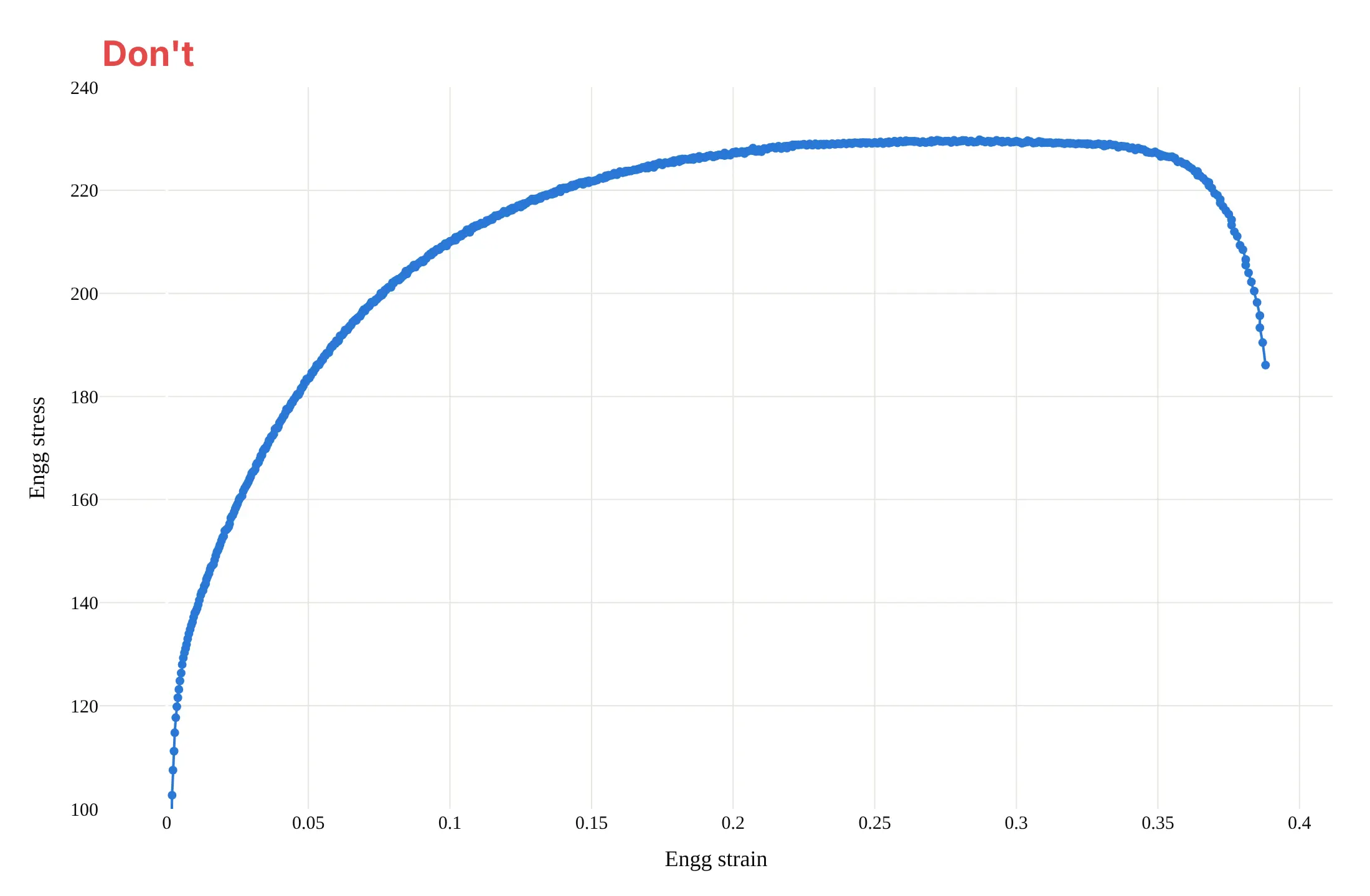
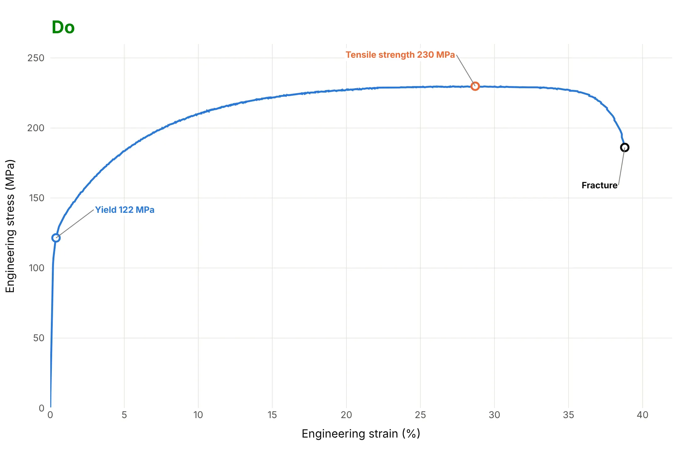
A stress-strain curve is read for numbers, so most of the work is in the axes, the units and the landmarks. Here is the aluminum test both ways, in the same color.
Don't keep the file's raw column names as axis titles, leave out the units, show strain as a fraction with no label, put a marker on every one of the 664 points, use a serif font, start the y axis at 100 so that the elastic start and the yield are cut off, or mark nothing:
Do write the axis titles with units, start both axes at zero so the stiffness and the yield are visible, draw one thin line, and label the yield strength, the tensile strength and the fracture with their values:
Checklist
Do
- Put strain on the x axis in percent and stress on the y axis in MPa, both from zero.
- Say whether the curve is engineering or true stress and strain, in the title or the axis titles.
- Say how the yield strength was read (0.2% offset, or upper and lower yield point) and how strain was measured.
- Plot every repeat specimen, not one chosen curve, when you compare materials.
- Stop a true stress curve at necking, or draw the rest dotted.
- Label the yield strength, tensile strength and fracture strain with values.
Don't
- Cut the x axis at 5% to make a flat curve look tall. The elastic region and the yield point sit at the very start.
- Read a modulus off a curve whose strain came from crosshead travel. It includes the machine's own flex, so the slope comes out low.
- Compare curves measured at different strain rates without saying so, as the polycarbonate example shows.
- Draw the full true stress curve past the neck as if it were measured.
More stress-strain curve examples
Five more charts built from real public tensile tests, each with its source, the technique that makes it work and a prompt to rebuild it.
1. Ten tests of one aluminum sheet at five angles
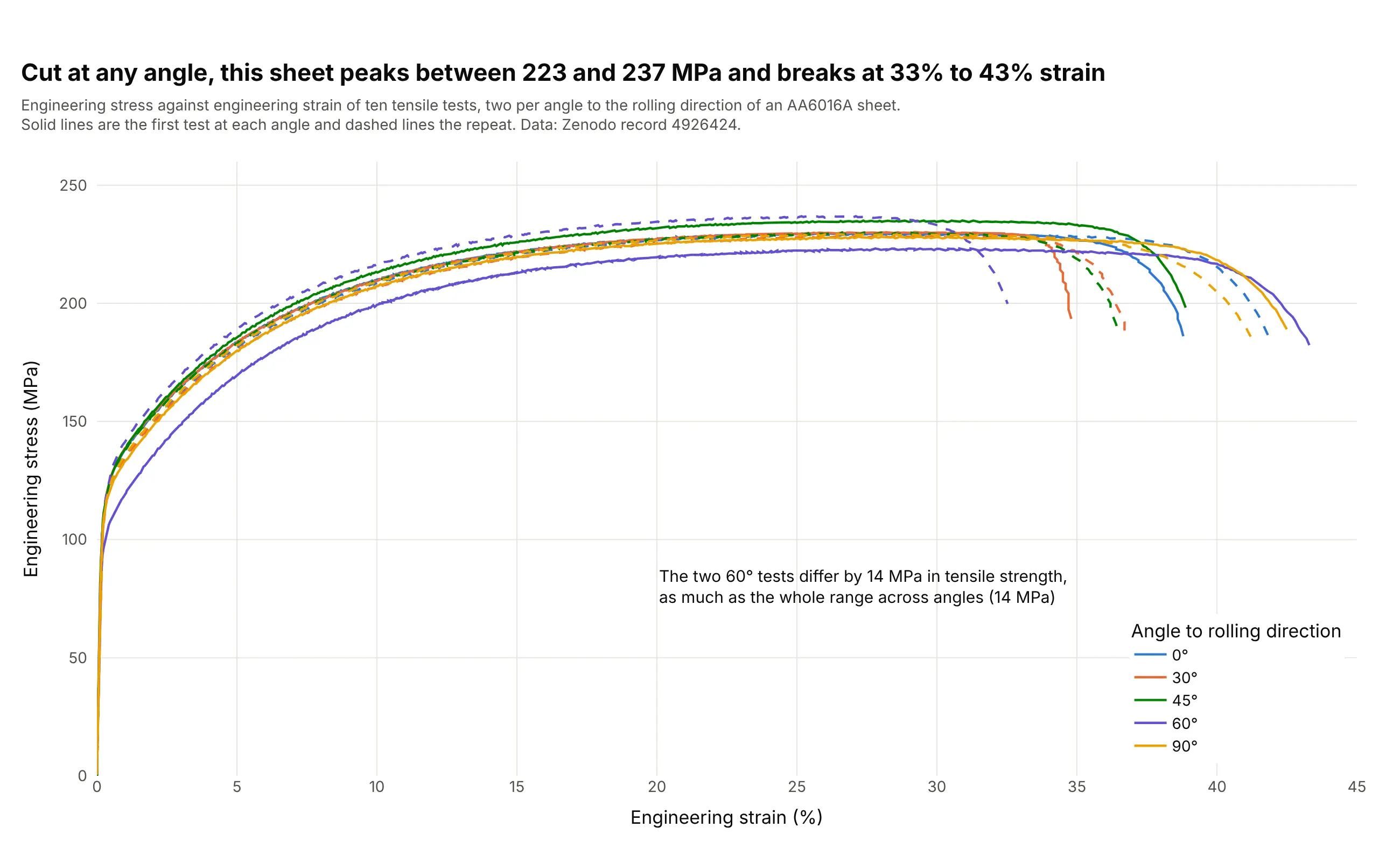
Cut at any angle to the rolling direction, the sheet peaks between 223 and 237 MPa and breaks at 33% to 43% strain. The two 60° tests are the lowest and highest of all ten, so the scatter between repeats is as large as the effect of the angle. Data: Zenodo record 4926424 (CC BY 4.0).
Tip: draw the repeat of each test as a dashed line in the same color, so the reader can judge the scatter before reading anything into a difference.
Get the data from Zenodo record 4926424 (tensile tests of Surfalex HF AA6016A sheet, https://doi.org/10.5281/zenodo.4926424):ten folders "test <angle>-<repeat>", each with a "voltage data" CSV with columns Engg stress (MPa) and Engg strain(a fraction, from digital image correlation).Build a plotly line chart of engineering stress against strain (%) for all ten tests, one color per angle,the first test solid and the repeat dashed, stopping each curve where the stress drops at fracture, with atitle that gives the range of tensile strength.
2. Nine copper alloys compared by yield strength
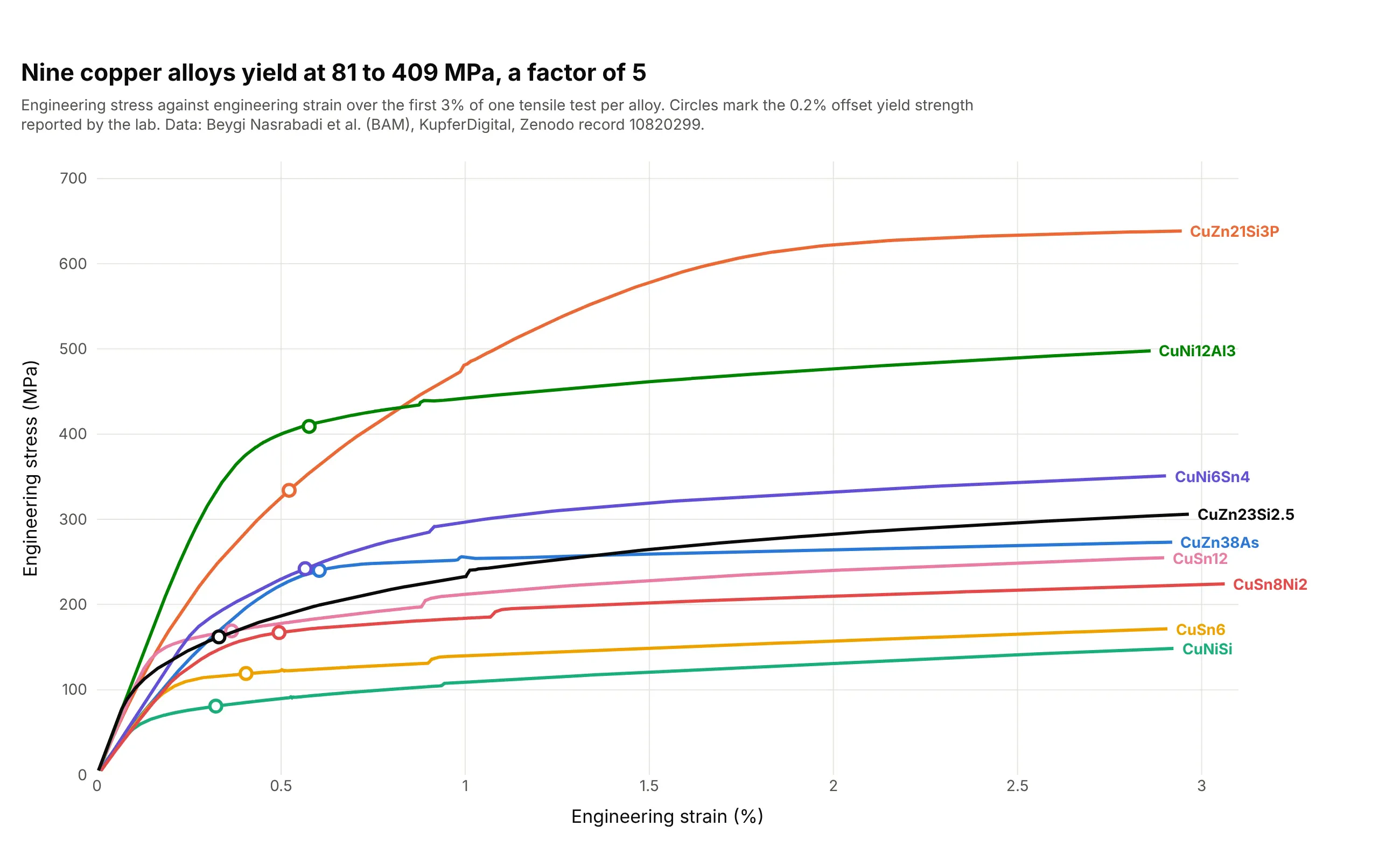
The nine alloys yield between 81 MPa (CuNiSi) and 409 MPa (CuNi12Al3), a factor of 5, and the circles on each curve are the lab's own 0.2% offset values. The strain sensor only works up to 3%, so the tensile strength and fracture come from the lab's summary table. Data: Beygi Nasrabadi et al. (2024), KupferDigital, Bundesanstalt für Materialforschung und -prüfung (BAM, the German federal institute for materials research and testing), Zenodo record 10820299 (CC BY 4.0).
Tip: when the x axis is cut to the part that was measured well, say so in the subtitle and take the rest of the numbers from the report, instead of stretching a poor signal across the whole chart.
Get the data from Zenodo record 10820299 (KupferDigital tensile tests of cast copper alloys, https://doi.org/10.5281/zenodo.10820299):the Tensile test/Primary data/*.lis files (tab-separated, decimal comma, a header with the alloy in "Werkstoff"and the lab's Dehngrenze Rp0.2, then a table Zeit, Weg, Kraft, Dehnung (%), Spannung (MPa) after "[Daten]").Make a plotly line chart of Spannung against Dehnung for the first specimen of each alloy over thefirst 3% of strain, one color per alloy, with a circle at the Rp0.2 value on each curve and the alloy name at theend of each line.
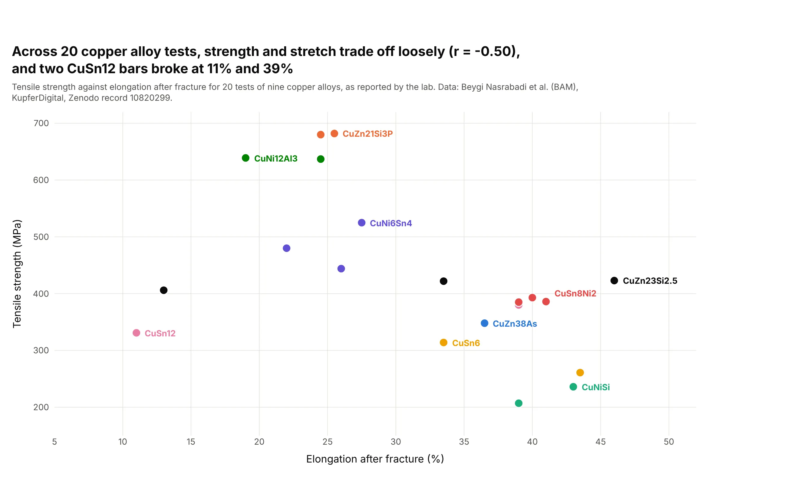
Another way to see it: the lab's tensile strengths and elongations for all 20 tests, as a scatter plot. Strong alloys tend to stretch less (correlation of -0.50), but two CuSn12 bars broke at 11% and 39%, so alloy name alone doesn't set the ductility of a cast bar:
3. Polycarbonate pulled at five speeds
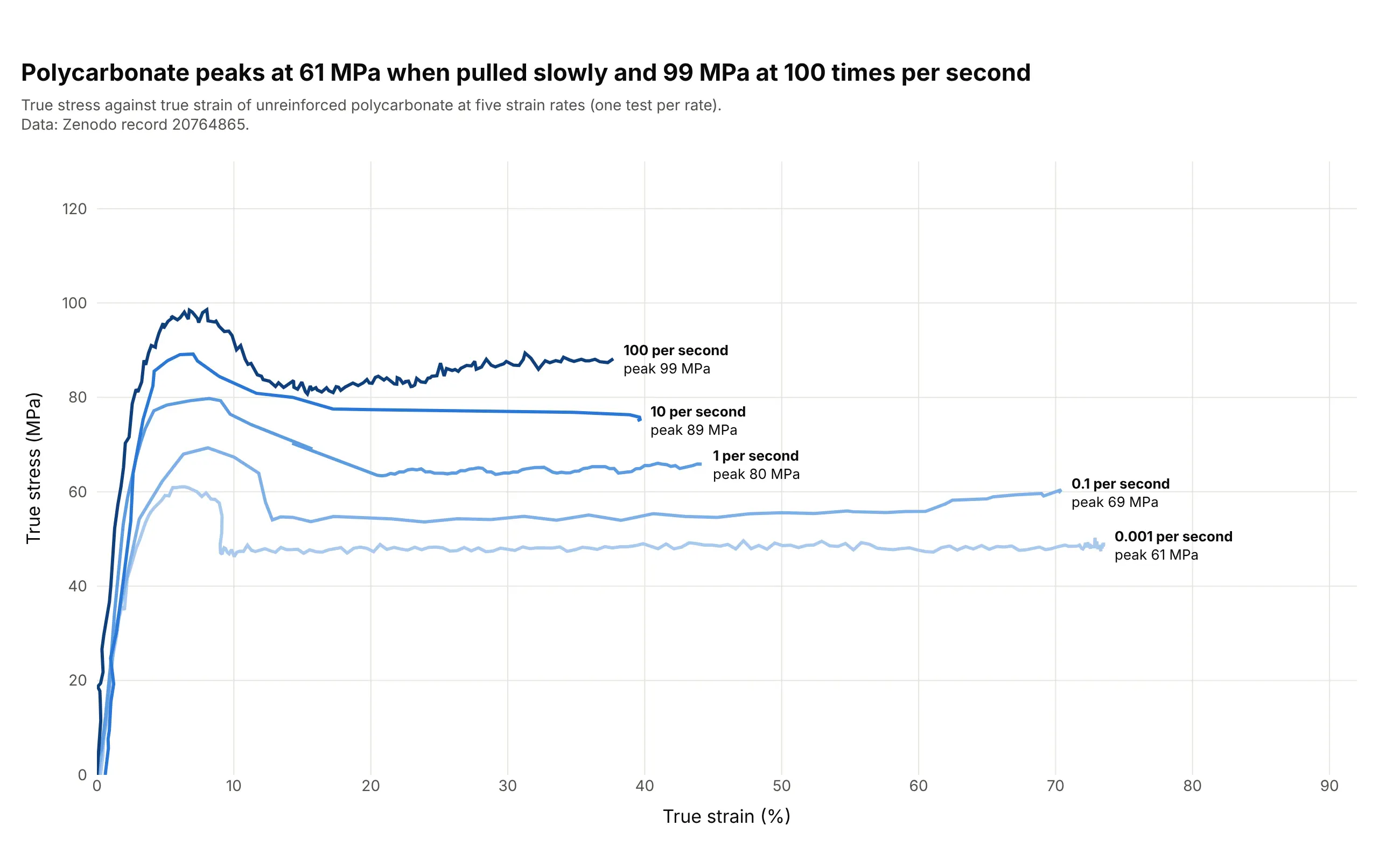
Polycarbonate peaks at 61 MPa when pulled slowly (0.001 per second) and 99 MPa at 100 per second, and every curve drops after its peak to a plateau as the plastic starts to flow. Because the curve changes with speed, a polymer's curve has to be quoted with its strain rate. Data: Zenodo record 20764865 (CC BY 4.0), true stress and true strain at five strain rates.
Tip: use sequential shades from light to dark for an ordered variable like speed, and put the label and the peak value at the end of each line.
Get the data from Zenodo record 20764865 (analyzed tensile data of polycarbonate, https://doi.org/10.5281/zenodo.20764865):the sheet PC_TensileCurve of PC_StressStrainCurves.xlsx with, for each strain rate (0.001, 0.1, 1, 10 and 100 per second),columns t (s), strain (mm/mm) and stress (MPa).Build a plotly line chart of true stress against true strain (%) for the five rates in sequential bluesfrom light for the slowest to dark for the fastest, with each line labeled with its rate and peak stress.
4. Rubber and polyethers stretched to 1,000%
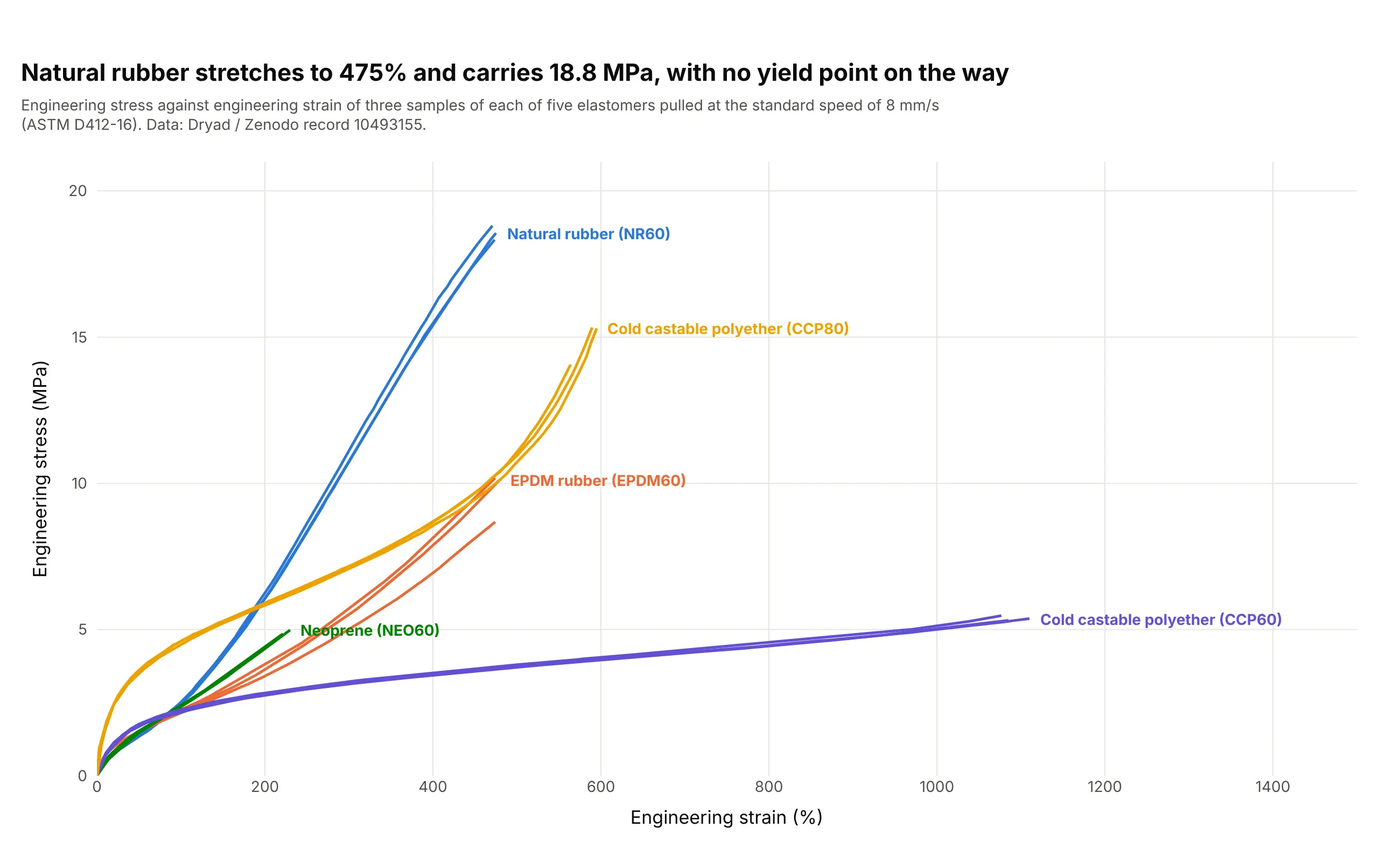
Natural rubber stretches to 475% and carries 18.8 MPa, while the softer polyether (CCP60) stretches to 1,110% and carries only 5.5 MPa. None of the five has a yield point or a straight elastic region, so the whole curve is what you quote. Data: Dryad / Zenodo record 10493155 (CC0), tests to the ASTM D412-16 standard for rubber. EPDM is ethylene propylene diene monomer rubber.
Tip: let the x axis run to the largest strain (here 1,500%) and put the labels at the line ends, so the curves that stop early don't leave the chart looking empty.
Get the data from Dryad / Zenodo record 10493155 (elastomer tensile tests to ASTM D412-16, https://doi.org/10.5061/dryad.kd51c5bbw):the Excel workbook with one sheet per material (NR60, EPDM60, NEO60, CCP60, CCP80) and, for each sample, a column ofstrain (%) and one of engineering stress (MPa), with the speed in the column heading.Build a plotly line chart of the three samples at the standard speed (8 mm/s) of each material, one color permaterial, with the material name at the end of its lines and the highest stress in the title.
5. 192 steel coupons, one yield strength each
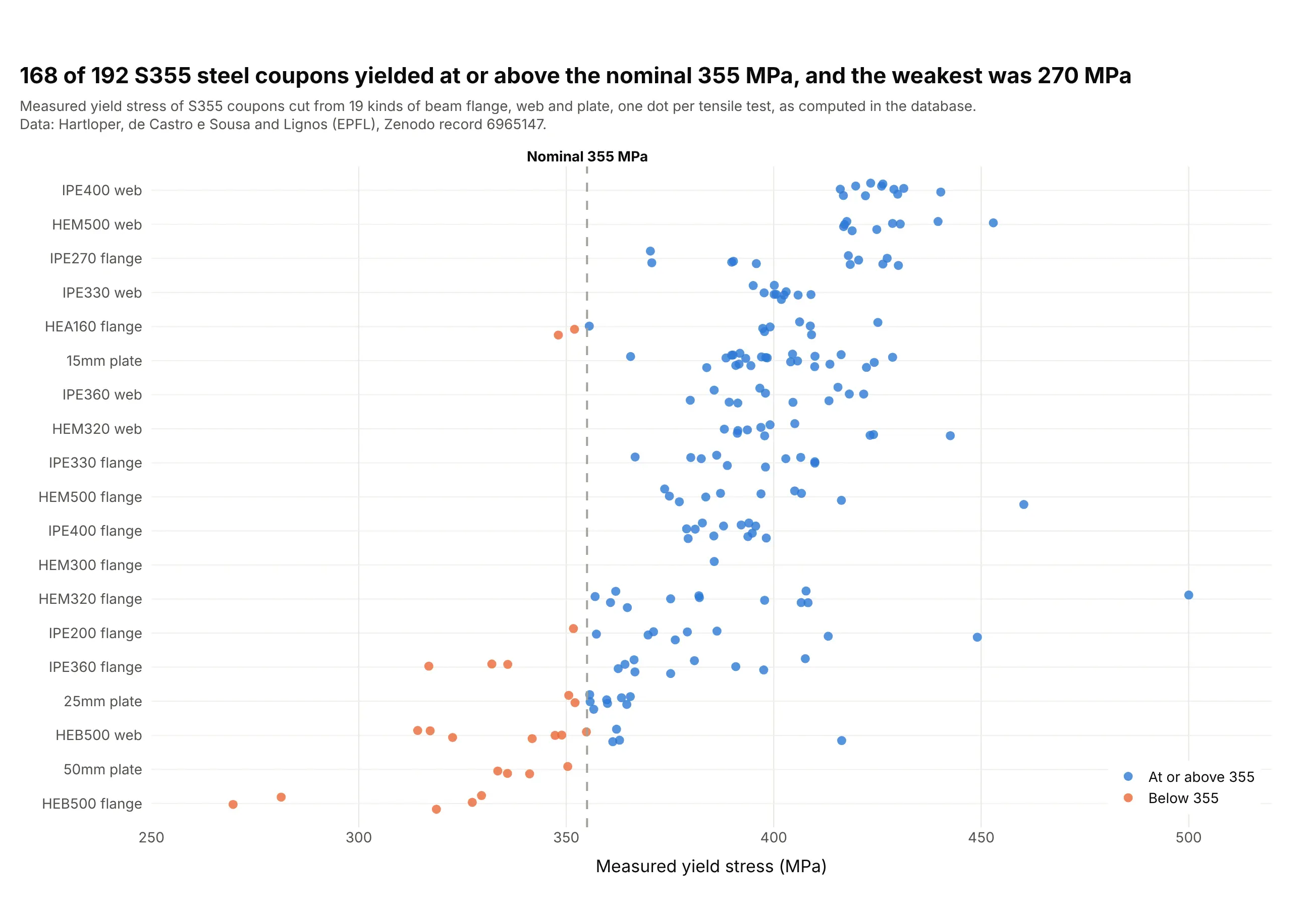
S355 steel is sold with a nominal yield strength of 355 MPa, and in this database 168 of 192 coupons were at or above it while 24 were below, down to 270 MPa for a HEB500 beam flange. The spread between parts is large, from a median of 319 MPa for the HEB500 flange to 426 MPa for the IPE400 web, so a single curve doesn't represent a steel grade. Data: Hartloper, de Castro e Sousa and Lignos (EPFL), Zenodo record 6965147 (CC BY 4.0), the database's summary table, with the yield stress computed by the authors.
Tip: sort the rows by median and jitter the dots vertically, so the spread, the trend and the specification line all read at once. This is a strip chart.
Get the data from Zenodo record 6965147 (database of coupon tests for structural metallic materials, https://doi.org/10.5281/zenodo.6965147):Overall_Summary_2022-08-30_v1-0-0.csv with columns grade, source, fy_n__mpa_ (the nominal yield strength) andyield_stress__mpa_ (the measured yield strength).Build a plotly strip chart of yield_stress__mpa_ for the rows with grade S355 and a nominal yield of 355, leaving outthe "C/s" sources, one row per source ordered by median, blue dots at or above 355 and orange below,a dashed line at 355 and a title with the share of coupons at or above it.
FAQ
Options to customize
A stress-strain curve in Plotly is a scatter line with computed landmarks, so these are the options that matter most. The full lists are in the scatter trace reference and the layout reference.
- go.Scatter(mode="lines") or go.Scattergl: the curve itself, with WebGL for hundreds of thousands of points.
- line.width, line.dash: a 3 px solid line for the main curve and dashed lines for the elastic and offset lines or for repeat tests.
- np.polyfit over the rising points: the elastic slope, the Young's modulus, fitted between two stress levels.
- add_shape(type="line") or a second go.Scatter trace: the 0.2% offset line, the same slope shifted right by 0.2% strain.
- mode="markers+text" with marker.size and textposition: the yield, tensile strength and fracture points with labels.
- add_annotation with ax and ay: labels with leader lines that state the value, such as "Yield strength 122 MPa".
- add_vrect: shaded phases, such as uniform stretching and necking, behind the curve.
- xaxis.rangemode="tozero", yaxis.rangemode="tozero": both axes from zero so the stiffness and the yield are visible.
- xaxis.type="log", yaxis.type="log": log-log axes for the Hollomon fit of the true curve.
- customdata and hovertemplate: the specimen name, strain and stress in the hover label of every curve when you overlay many tests.
- fill="toself": the area under the curve, the toughness, shaded.
- make_subplots: small multiples of different materials, each with its own axes, as in the shapes figure.