
Chris Parmer
November 15, 2026
Sparklines - A Complete Guide
TL;DR
- A sparkline is a very small line chart drawn without axes or labels, small enough to sit inside a sentence, a table cell or a card, so that the shape of a number's history is visible exactly where the number is. Edward Tufte, who named it, called sparklines "data-intense, design-simple, word-sized graphics".
- Sparklines are also known as word-sized graphics, datawords and inline charts, and are similar to line charts, small multiples and the sparkline that sits under the number on a key performance indicator (KPI) card (see the KPI card guide).
- A grid of sparklines is a set of subplots, the panels of a small multiples chart, with the axes, ticks and gridlines stripped away, so you can scan a dozen or more series at once for their shapes and read each one's latest value from its header.
- Three choices decide whether a sparkline helps: what to mark (the last value, the high and low, a gray band for the normal range), whether rows share a y scale or each get their own, and the aspect ratio, which should make the line's typical slope about 45 degrees.
- You can make a sparkline with Plotly from a go.Scatter trace on axes that are hidden: one tiny figure per row in a Dash app, or one figure with a subplot per row. A short helper function is below.
What is a sparkline?
Sparklines look like this:
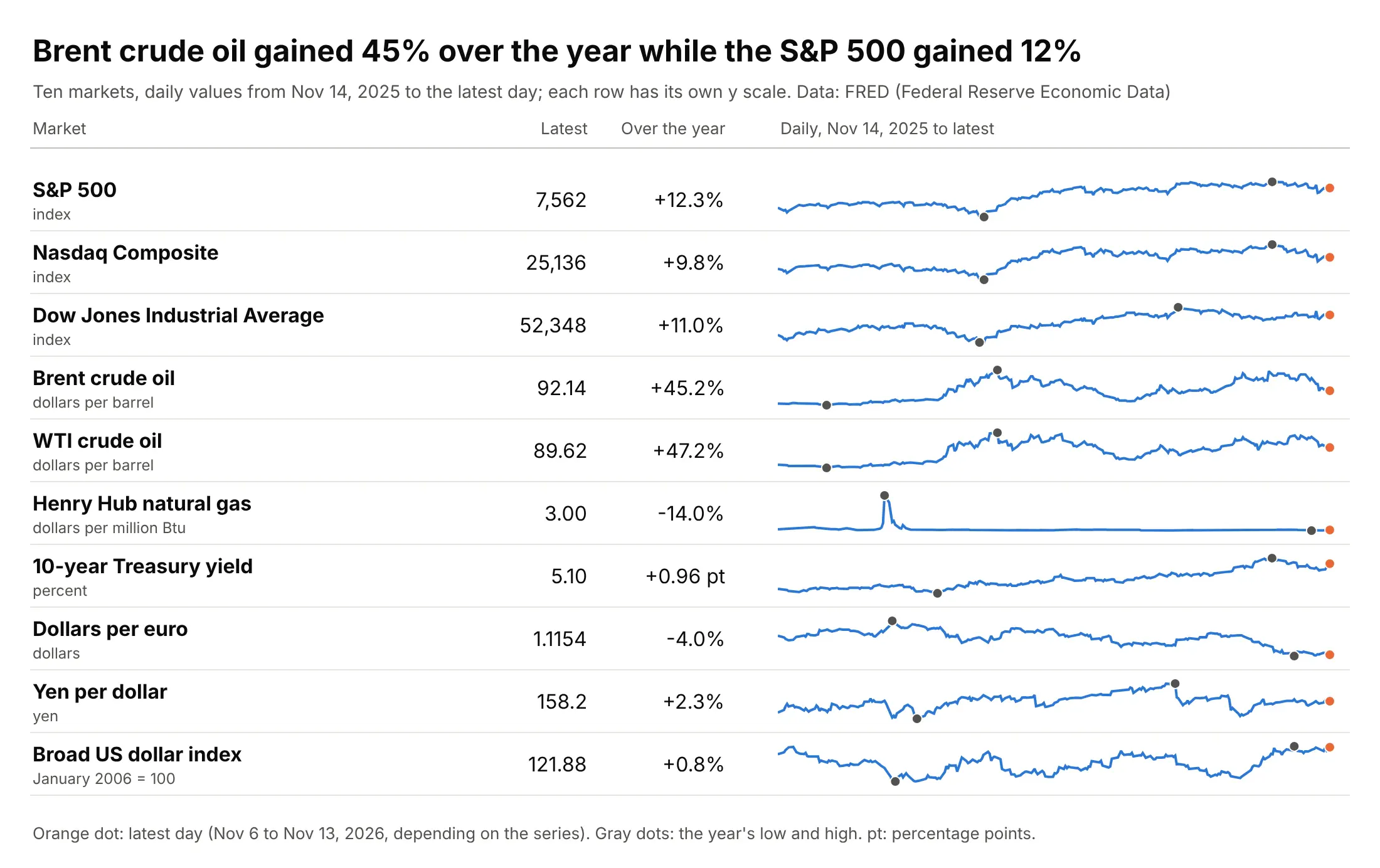
Data: FRED (Federal Reserve Economic Data), the St. Louis Fed's database: S&P Dow Jones Indices, Nasdaq, the US Energy Information Administration (EIA), and the Federal Reserve. Values from November 14, 2025 to the latest day (November 6 to 13, 2026, depending on the series). The change in the 10-year Treasury yield is in percentage points (pt), because a percent change of a rate is easy to misread.
How do you read a sparkline? In the example above, notice these things:
- Each row is one market, and the number on the left is its latest value, so the sparkline only has to show what the number can't: the path the value took over 12 months. The S&P 500 index, which tracks 500 large US companies, is at 7,562 and dipped in March 2026 before climbing back.
- The lines have no axes, so you read their shape and not their height, and every row has its own y scale. Brent crude oil rose from $63.45 a barrel on November 14, 2025 to $92.14 on November 11, 2026 (up 45.2%), and the line fills its row.
- The gray dots mark the year's low and high, and the orange dot marks the latest day. Brent's high was $138.21 on April 7, 2026, well above where it ends, which the number 92.14 alone wouldn't tell you.
- One extreme day can flatten everything else in a row. Henry Hub natural gas reached $30.72 per million British thermal units (Btu) on January 23, 2026, ten times its latest $3.00, so the rest of the year is a flat line.
It's often used for charts like these:
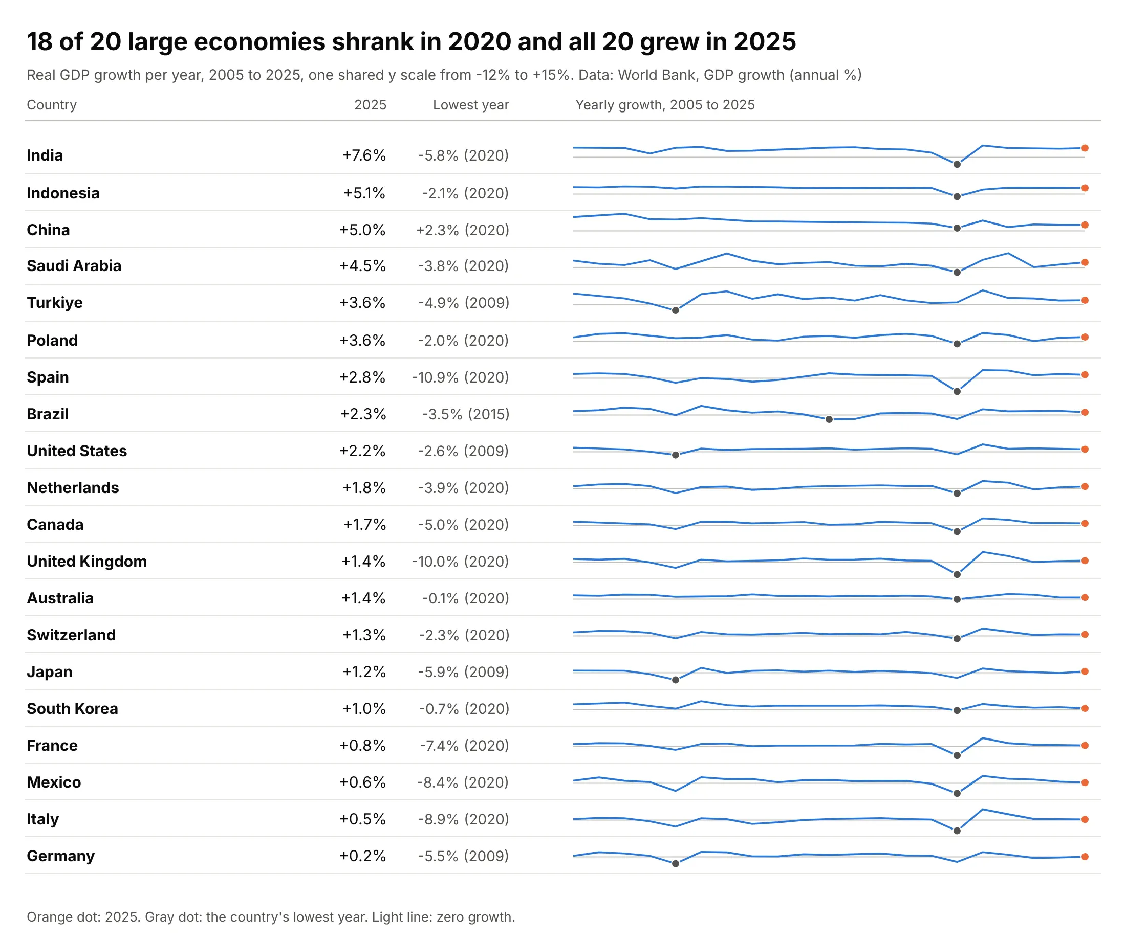
Tables of many items. A table of 20 countries' gross domestic product (GDP) growth shows that 18 of the 20 economies shrank in 2020 and all 20 grew in 2025, which a column of 21 yearly numbers per country would bury. Data: World Bank, GDP growth (annual %).
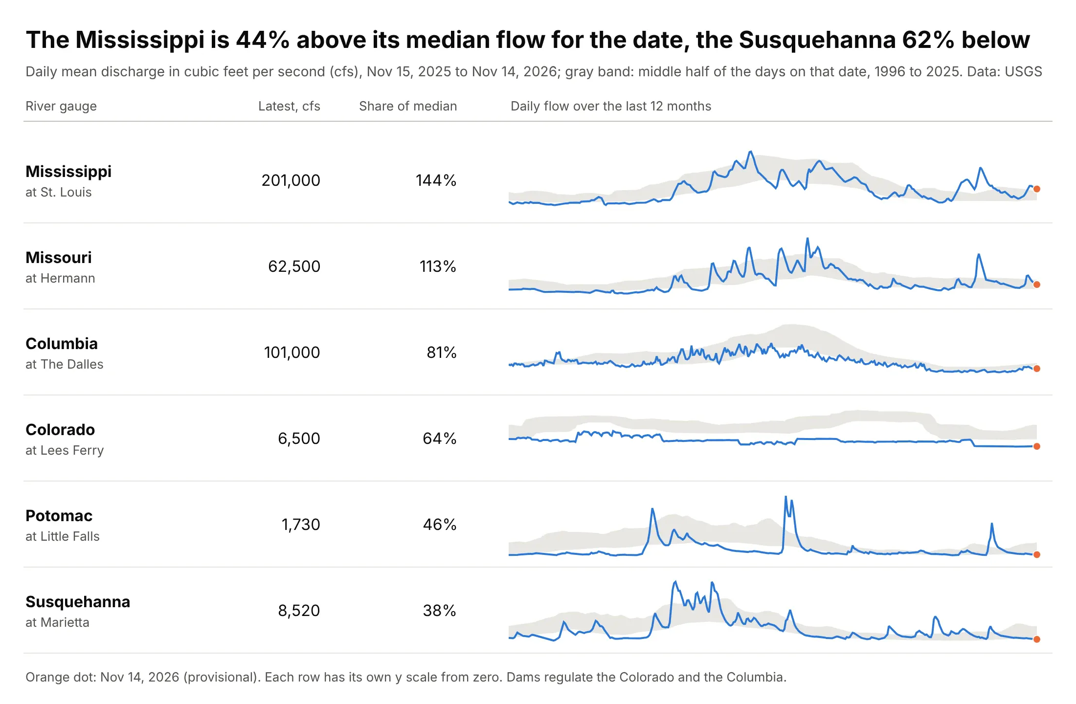
A number against its normal. Tufte's own medical example drew a patient's glucose readings against a gray band for the normal range, and a river gauge works the same way: the Mississippi at St. Louis is flowing at 144% of its median for the date and the Susquehanna at Marietta at 38%. Data: US Geological Survey (USGS), National Water Information System.
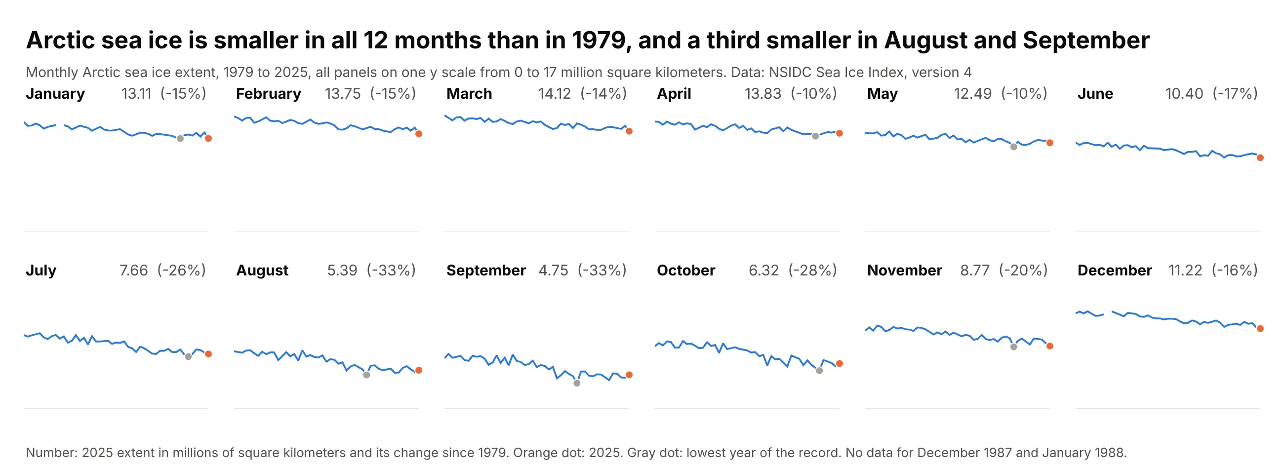
A grid of many series. Arctic sea ice extent in each of the 12 months of the year shrank between 1979 and 2025, by about 10% in April and May and by a third in August (-33%) and September (-33%), and a grid of 12 panels shows all 12 lines at once with the number in each header, where a table would need 47 yearly values per month. All panels share one y scale because they have the same unit and the gap between March (14.12 million square kilometers in 2025) and September (4.75) is part of the picture. Data: National Snow and Ice Data Center (NSIDC), Sea Ice Index, version 4 (extent is the area of ocean with at least 15% ice cover).
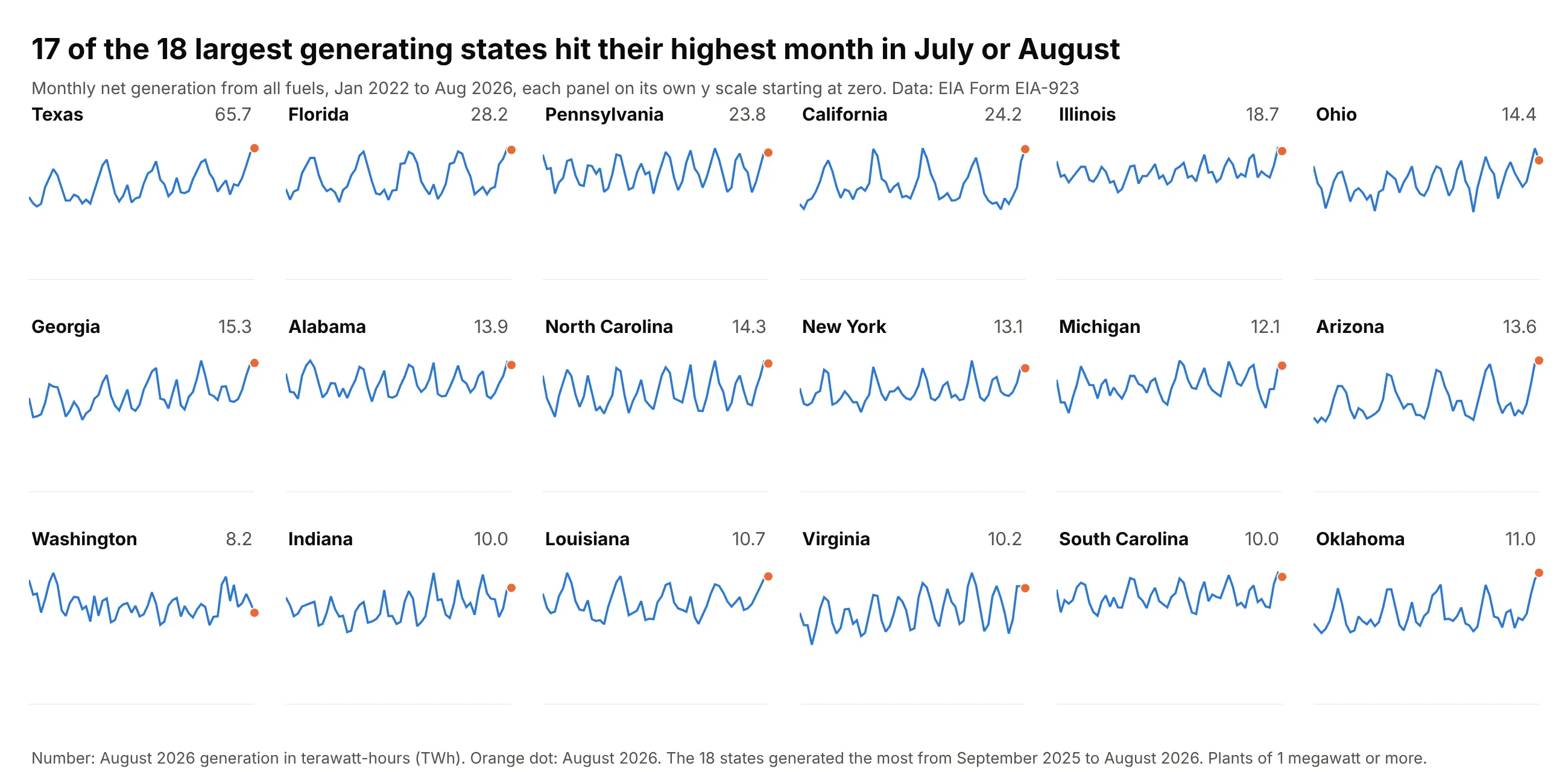
A grid of regions. In 17 of the 18 states that generated the most electricity over the last year, the highest month between January 2022 and August 2026 was a July or an August, the summer peak, and Indiana's was January 2025. Each panel has its own y scale starting at zero, because Texas (65.7 TWh in August 2026) is several times Oklahoma (11.0) and the question is about the shape of the year. Data: US Energy Information Administration (EIA), Form EIA-923.
A short history
Tufte had shown a compact style of time series, which he called "intense continuous time-series", in his 1983 book The Visual Display of Quantitative Information, and he named the sparkline in a draft chapter on his website in 2004 and in Beautiful Evidence (Graphics Press, 2006, pages 46 to 63). His chapter "Sparklines: Intense, Simple, Word-Sized Graphics" opens with a patient's blood glucose as a word and a number, then adds the last 80 readings, a color accent on the latest one and a gray band for the normal range. His financial example is a table with a year of the euro's daily dollar price in each row, with red dots on the oldest and newest rates and blue dots on the yearly low and high. He argued that a year-long daily history "reduces recency bias", the habit of overweighting the latest events, and that the aim is to be "approximately right rather than exactly wrong". Software had the idea slightly earlier: Peter Zelchenko wrote an "inline-chart" feature for the QuoteTracker stock program in 1999, and Microsoft added sparklines to Excel 2010 (Wikipedia).
Here is the idea of his euro table redrawn with Plotly and a year of Federal Reserve exchange rates, using his color code. This is a redraw with new data, not a copy of his figure:
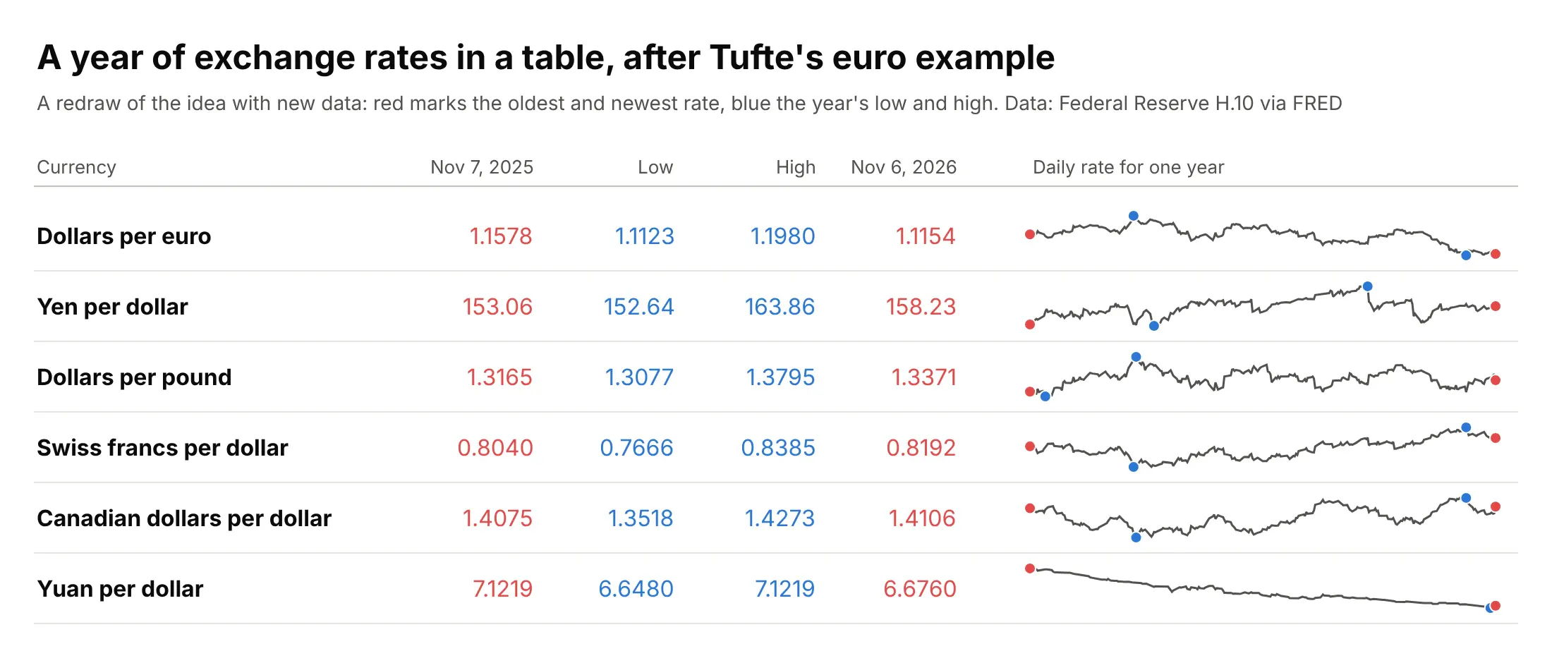
Data: Board of Governors of the Federal Reserve System, H.10 Foreign Exchange Rates, via FRED.
What to mark on a sparkline
A sparkline with no marks answers one question, whether the value is going up or down. Each mark you add answers another, and the three below cover most needs. Here is one river drawn four ways:
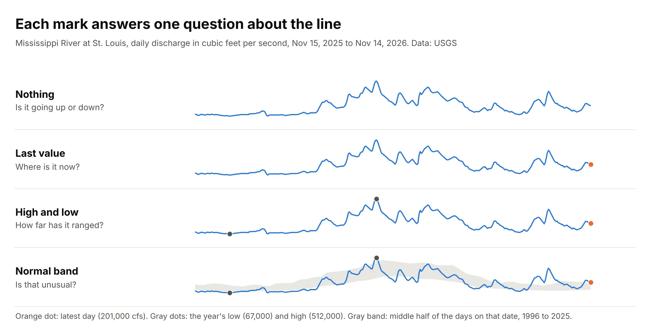
Data: USGS daily mean discharge of the Mississippi River at St. Louis, November 15, 2025 to November 14, 2026.
The last value. A dot on the latest point ties the line to the number beside it, as Tufte did with a color accent. Use a color that no other element of the row uses.
The high and low. Two dots show how far the value has ranged, and the rest of the row can then be read against them. The Mississippi's low was 67,000 cubic feet per second (cfs) on December 17, 2025 and its high 512,000 on May 1, 2026. A cfs is a cubic foot of water, about 7.5 US gallons, passing a point every second.
A normal band. A gray band behind the line shows what is typical for the date, so the line answers "is that unusual?". The band here comes from 30 years of daily flows, 1996 to 2025. For each calendar date it holds the 25th to the 75th percentile of the flows within 7 days of that date, which means a quarter of those days were below the band, a quarter above it and half inside. Where the line leaves the band the river is higher or lower than in most years, and the share of the median (the middle value of the same days) puts a number on it: 201,000 cfs against a median of 139,500 is 144%.
Shared or independent y scales
Every sparkline has a y scale even though it isn't drawn, and you choose it. With independent scales each row fills its own height, so the shapes are easy to read, but a row that barely moved looks as dramatic as one that doubled. With one shared scale the heights compare across rows, and a quiet row looks quiet. Here are five markets both ways, with the shared version drawn as percent change since November 14, 2025:
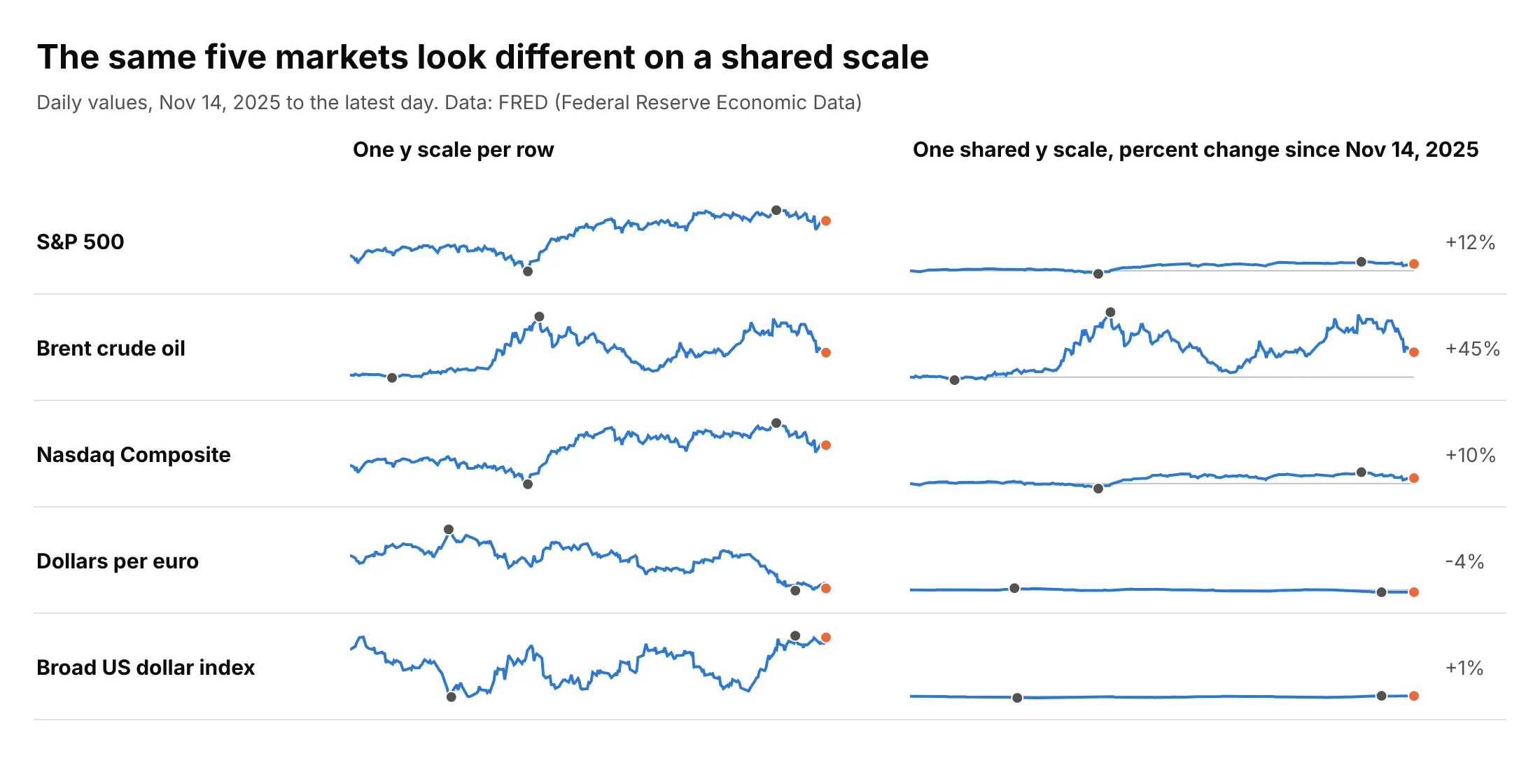
Data: FRED (Federal Reserve Economic Data), Nov 14, 2025 to the latest day.
Use independent scales when the rows have different units (a stock index, an oil price and an exchange rate), because a shared axis would make no sense, and when the question is about shape. Use a shared scale when the rows have the same unit and the question is about size, such as the temperatures in example 1 below or the growth rates in the GDP table above. When one row dominates a shared scale, as Brent does here, say so in the subtitle or give it its own row.
Sparklines, subplots and small multiples
A grid of sparklines is a grid of subplots. In Plotly a subplot is one panel of a figure with its own pair of axes (make_subplots creates a grid of them), and a small multiples chart is a grid of subplots that all show the same kind of chart for different slices of the data, such as one panel per month or per state. Take a small multiples chart, remove the ticks, the gridlines and the axis labels, put the name and the latest value in each panel's header, and you have a sparkline grid. Here is one set of US Treasury yields drawn both ways:
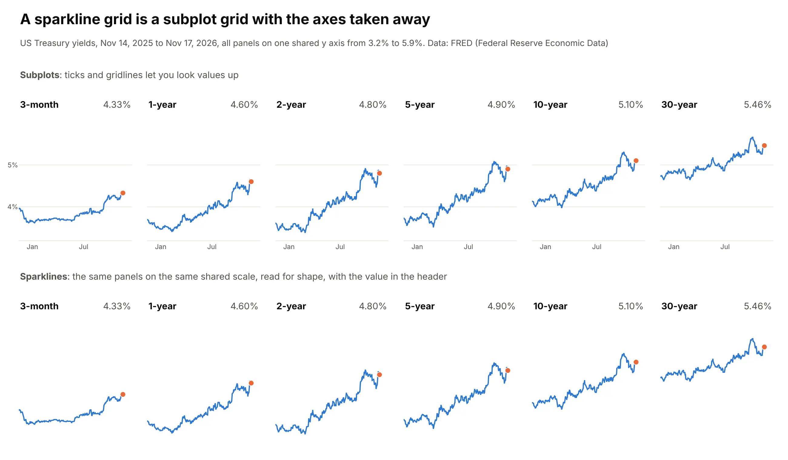
Data: FRED (Federal Reserve Economic Data), Board of Governors of the Federal Reserve System, H.15 Selected Interest Rates, daily constant-maturity yields.
The difference is what the reader does with it. Subplots with axes are for looking values up, such as the date a yield crossed 5%, and they need room for the tick labels. Sparklines are for scanning for shapes across many panels. Keep the axes when the exact value matters, and drop them when the shape matters and the header holds the number.
The choice of axes matters more in a grid than in a table, because the eye compares neighboring panels:
- Share the y axis when the panels have the same unit and the question is about size. In the figure above, all six panels use one scale, so the 3-month yield visibly rose less than the 30-year (from 3.95% to 4.33%, against 4.74% to 5.46%). Use shared_yaxes=True in make_subplots, or let px.line do it, since Plotly Express shares the axes of every facet by default.
- Give each panel its own y axis when the sizes differ a lot and the question is about shape. The state electricity grid above does this, because Texas generates several times what Oklahoma does. Independent scales mislead when the reader assumes the panels are comparable: a flat series stretched to fill its panel looks as dramatic as a volatile one. Start each y axis at zero for quantities such as generation, say in the subtitle that the scales differ, and put the size in the header.
- Always share the x axis (the same dates or the same years in every panel), so that a rise in one panel lines up with a rise in the next.
To build a grid, use make_subplots with shared_yaxes=True and add one trace per panel, or call px.line with facet_col and facet_col_wrap, and then hide the axes. Both snippets run on a file with the columns name, date and value:
import pandas as pdimport plotly.express as pximport plotly.graph_objects as gofrom plotly.subplots import make_subplotsdf = pd.read_csv("treasury.csv", parse_dates=["date"]) # columns: name, date, valuenames = ["3-month", "1-year", "2-year", "5-year", "10-year", "30-year"]# Option 1: make_subplots, one shared y axis for every panel, panel names as subplot titlesfig = make_subplots(rows=1, cols=6, shared_yaxes=True, subplot_titles=names, horizontal_spacing=0.02)for i, name in enumerate(names, start=1):g = df[df.name == name]fig.add_trace(go.Scatter(x=g.date, y=g.value, mode="lines", line=dict(width=2)), row=1, col=i)fig.update_xaxes(visible=False)fig.update_yaxes(visible=False)fig.update_layout(showlegend=False, height=140, margin=dict(l=10, r=10, t=30, b=10), plot_bgcolor="white")fig.show()# Option 2: px.line with facets, wrapped to a new row every 3 panels (the axes are shared by default)fig = px.line(df[df.name.isin(names)], x="date", y="value", facet_col="name", facet_col_wrap=3,category_orders={"name": names}, height=300)fig.update_xaxes(visible=False)fig.update_yaxes(visible=False)fig.for_each_annotation(lambda a: a.update(text=a.text.split("=")[-1])) # "name=10-year" becomes "10-year"fig.show()
For independent y axes, pass shared_yaxes=False to make_subplots, or facet_col_wrap with fig.update_yaxes(matches=None) in Plotly Express. The sea ice and electricity grids in this guide are make_subplots figures with 12 and 18 panels.
Sparklines in tables, KPI cards and small multiples
A sparkline is most useful as one column of a table. A quote board, a league table or an inventory list already has a label and a number per row, and the sparkline adds the history without adding a chart to look at. Keep the rows aligned, put the sparkline last, and align the numbers to the right so they can be compared.
On a KPI card, the sparkline goes under the big number and answers whether this month is unusual, as example 3 below shows. The card guide covers the delta and its colors. If you find yourself adding axes and gridlines to the sparkline so that readers can look values up, you need a full chart, and a grid of them with shared axes is a small multiples chart.
Alternatives to a sparkline
Here's the same five markets drawn six ways. Some are better for the question, some worse, some just different:
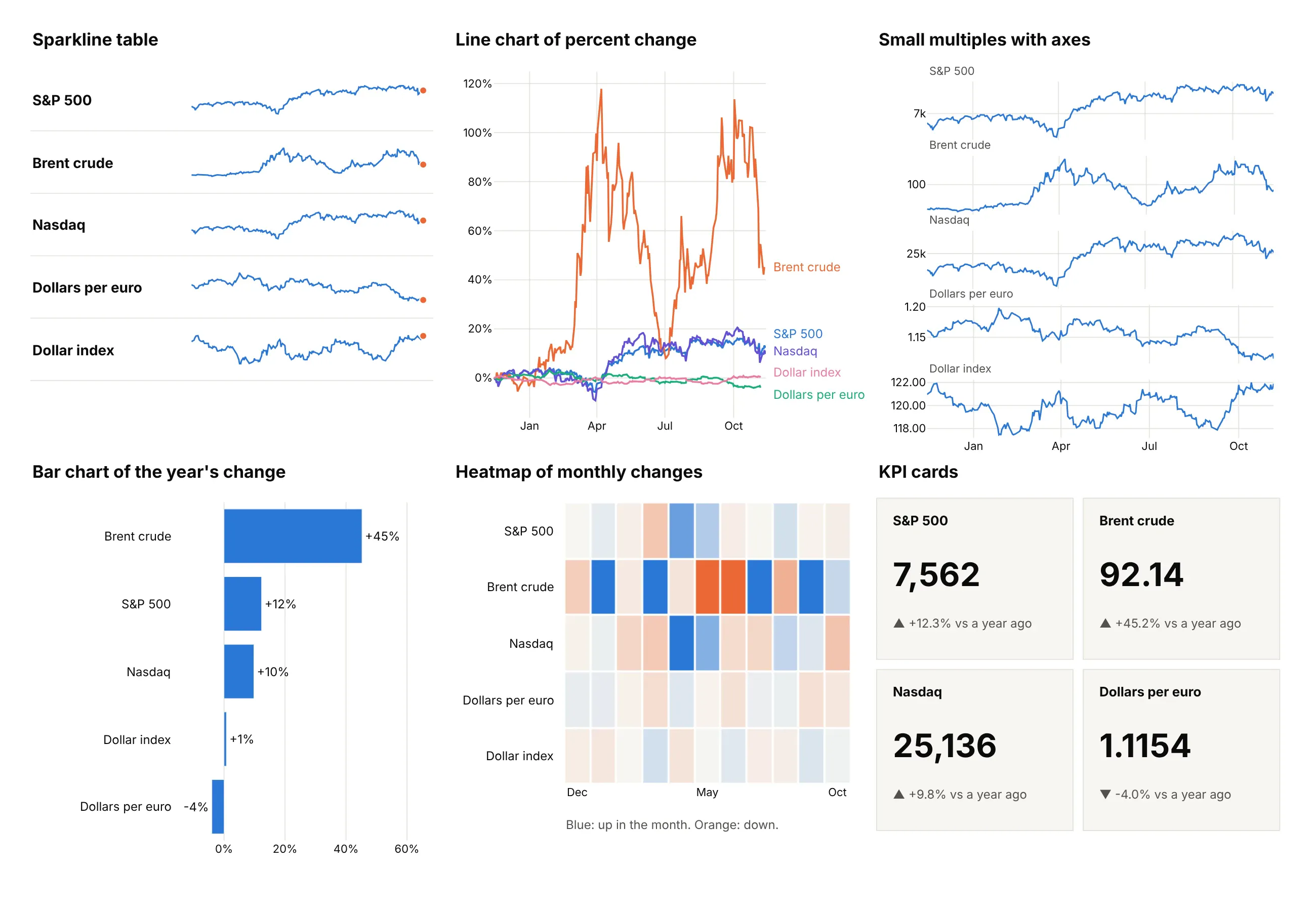
- Line chart of percent change (worse for more than three series). Putting everything on one axis lets you compare size, but Brent's swings squash the dollar and the euro into the bottom, and the labels collide.
- Small multiples with axes (better when readers need to look values up). Each panel has ticks and gridlines, so you can read that the S&P 500 stayed between about 6,300 and 7,800, at the price of a lot more space per row.
- Bar chart of the year's change (works too, for one number). It ranks the markets exactly (+45% for Brent, -4% for the euro) and hides the path, such as Brent's rise to $138.21 and fall back.
- Heatmap of monthly changes (different). It shows which months moved, such as Brent's large swings in both directions, using color instead of position, which is harder to read precisely.
- KPI cards (different). They put the latest number first and the change second and need a sparkline to show the history.
How to make a sparkline
With AI
ChatGPT, Claude Code, GitHub Copilot, Cursor and other AI tools are excellent at writing Plotly code. Name Plotly in the prompt, and say what goes in each column, what to mark and which y scale each row uses:
Make a plotly sparkline table from markets.csv (columns: name, date, value; one year of daily values for 10 markets).- One row per market with its name, the latest value with thousands separators, the change over the year as a signed percent, and a sparkline, all in one figure using one pair of hidden axes per row (go.Scatter in make_subplots, no ticks, no grid).- Each row has its own y scale. Draw the line in #2a78d6, an orange dot on the latest day and gray dots on the low and high.- Use Inter, a white background and a title that states the biggest change.- Check: print each market's latest value, change and the dates of its low and high.
With Plotly Studio
Plotly Studio is a product for creating data visualizations and Dash apps and for analyzing data with AI, available as a desktop app or embedded in Dash apps. Ask for a sparkline table the same way:
Show a table of the 20 largest economies with their latest GDP growth and a sparkline of growth for each year since 2005, all on one shared scale, with the lowest year marked, and a dropdown to sort by latest growth or by lowest year.
Make a sparkline in Python or JavaScript
This is the code AI tools write under the hood. A sparkline in Plotly is a go.Scatter trace on a pair of axes that you hide, so a tiny figure with no axes, margins or legend is the whole technique. This helper returns a go.Figure, and every example in this guide builds on the same idea:
import pandas as pdimport plotly.graph_objects as gofrom plotly.subplots import make_subplotsdef sparkline(dates, values, color="#2a78d6"):"""A sparkline in Plotly: one line, a dot on the latest value and every axis hidden."""fig = go.Figure(go.Scatter(x=dates, y=values, mode="lines", line=dict(color=color, width=2)))fig.add_trace(go.Scatter(x=[dates.iloc[-1]], y=[values.iloc[-1]], mode="markers",marker=dict(color="#eb6834", size=8), cliponaxis=False))fig.update_xaxes(visible=False)fig.update_yaxes(visible=False)fig.update_layout(width=240, height=48, margin=dict(l=2, r=8, t=4, b=4), showlegend=False,paper_bgcolor="white", plot_bgcolor="white")return figdf = pd.read_csv("markets.csv", parse_dates=["date"]) # columns: name, date, valuebrent = df[df.name == "Brent crude oil"]sparkline(brent.date, brent.value).show()
To put many sparklines in one figure, give each row its own subplot, which also gives it its own y scale. The row labels are annotations that point at each subplot's domain:
names = df.name.unique()fig = make_subplots(rows=len(names), cols=1, vertical_spacing=0.03)for i, (name, g) in enumerate(df.groupby("name", sort=False), start=1):fig.add_trace(go.Scatter(x=g.date, y=g.value, mode="lines", line=dict(color="#2a78d6", width=2)), row=i, col=1)fig.add_trace(go.Scatter(x=g.date.iloc[[-1]], y=g.value.iloc[[-1]], mode="markers",marker=dict(color="#eb6834", size=8), cliponaxis=False), row=i, col=1)fig.add_annotation(text=f"<b>{name}</b>", x=0, xref="paper", xanchor="right", xshift=-12,y=0.5, yref="y domain" if i == 1 else f"y{i} domain", showarrow=False)fig.update_xaxes(visible=False)fig.update_yaxes(visible=False)fig.update_layout(width=700, height=70 * len(names), margin=dict(l=190, r=20, t=10, b=10), showlegend=False)fig.show()
For a table with several text columns, as in the images in this guide, place everything by pixel instead: add each text with add_annotation and each sparkline on its own pair of axes whose domain is the rectangle you want. The folder's sparklib.py does this in about 150 lines and gives the Canvas.spark() and Canvas.bars() calls the examples use. To share one y scale, pass the same range to every row's y axis. A column sparkline, or a win/loss sparkline, is a go.Bar on the same hidden axes.
In JavaScript, plotly.js draws a sparkline the same way, and a table is a loop that gives each cell its own chart:
<table id="markets" style="border-collapse:collapse;font-family:Inter,Arial,sans-serif"></table><script src="https://cdn.plot.ly/plotly-4.1.1.min.js"></script><script>// Last value of each month from Nov 2025 to Nov 2026 (the last point is Nov 11 to 13), from FREDconst markets = {"S&P 500": [6849.09, 6845.5, 6939.03, 6878.88, 6528.52, 7209.01, 7580.06, 7499.36, 7489.72, 7686.14, 7651.54, 7580.07, 7561.67],"Brent crude oil": [64.07, 61.35, 72.25, 71.32, 126.69, 124.24, 92.88, 70.46, 96.95, 89.75, 115.91, 120.15, 92.14],"10-year Treasury yield": [4.02, 4.18, 4.26, 3.97, 4.3, 4.4, 4.45, 4.44, 4.75, 4.75, 5.29, 4.94, 5.1]};// One sparkline: a line, a dot on the last value and every axis hiddenfunction sparkline(div, y) {const last = y.length - 1;Plotly.newPlot(div, [{y: y, mode: "lines", line: {color: "#2a78d6", width: 2}},{x: [last], y: [y[last]], mode: "markers", marker: {color: "#eb6834", size: 8}, cliponaxis: false}], {width: 240, height: 48, margin: {l: 2, r: 8, t: 4, b: 4}, showlegend: false,xaxis: {visible: false}, yaxis: {visible: false}}, {staticPlot: true});}for (const [name, y] of Object.entries(markets)) {const row = document.getElementById("markets").insertRow();row.insertCell().textContent = name;row.insertCell().textContent = y[y.length - 1].toLocaleString();sparkline(row.insertCell(), y);}</script>
Make a sparkline table in Dash
For a live table, a Dash app can put a small dcc.Graph in each row of an html.Table, with staticPlot on so the sparklines don't capture the mouse. The sparkline() helper above is the only chart code, and the table is plain HTML:
from dash import Dash, dcc, htmlORDER = ["S&P 500", "Brent crude oil", "Henry Hub natural gas", "10-year Treasury yield", "Dollars per euro"]def change(name, v):"""Percent change for prices, change in percentage points (pt) for a yield."""if "yield" in name:return f"{v.iloc[-1] - v.iloc[0]:+.2f} pt"return f"{100 * (v.iloc[-1] / v.iloc[0] - 1):+.1f}%"def row(name):g = df[df.name == name].sort_values("date")v = g.valuereturn html.Tr([html.Td(name, style={"fontWeight": 600, "padding": "6px 24px 6px 0"}),html.Td(f"{v.iloc[-1]:,.2f}", style={"textAlign": "right", "padding": "6px 24px"}),html.Td(change(name, v), style={"textAlign": "right", "padding": "6px 24px"}),html.Td(dcc.Graph(figure=sparkline(g.date, v), config={"staticPlot": True}, style={"height": "44px"})),], style={"borderTop": "1px solid #e6e5e0"})app = Dash(__name__)app.layout = html.Div([html.H3("Markets over the last year"), html.Table(html.Tbody([row(n) for n in ORDER]))])app.run()
This is the app, running locally:
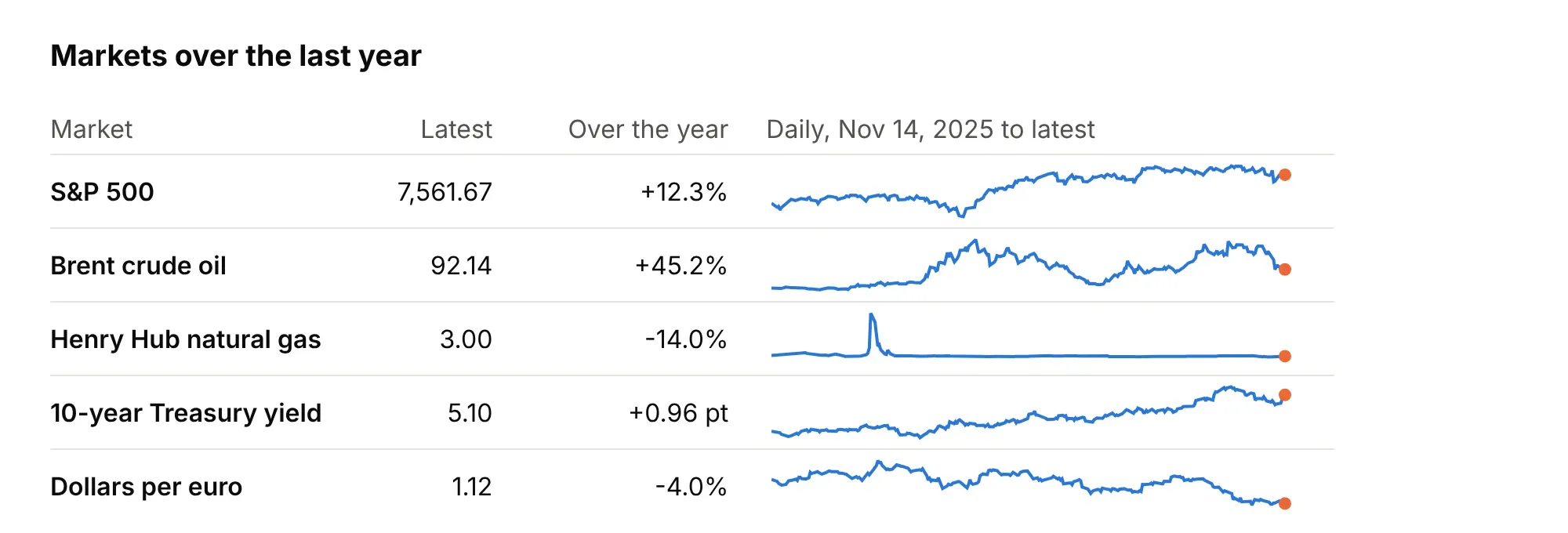
Sorting and filtering a table like this means rebuilding the rows in a callback. That is fast for tens of rows, and the benchmark in the FAQ shows where one figure per row stops being a good idea.
Share it
Every Plotly chart has a Share chart button (the cloud icon in its toolbar) that uploads it to Plotly Cloud and gives you a link. Only you can see it until you change its visibility.
For a live app, put the chart in a Dash app and publish it with the Plotly Cloud CLI. Coding agents can run these commands for you:
pip install "dash[cloud]"plotly user loginplotly app publish
If your data has to stay in your own cloud or data center, publish to Dash Enterprise instead.
Dos and don'ts
Most of the work in a sparkline table is deciding what to leave out. Here are five markets both ways, in the same blue.
Don't draw series in different units on one y scale (the S&P 500 at 7,562 leaves the others as flat lines at zero), keep axes, ticks and gridlines on every sparkline, print raw numbers such as 7561.67 and 0.122891, use a serif font and cramped rows, or leave the latest day unmarked:
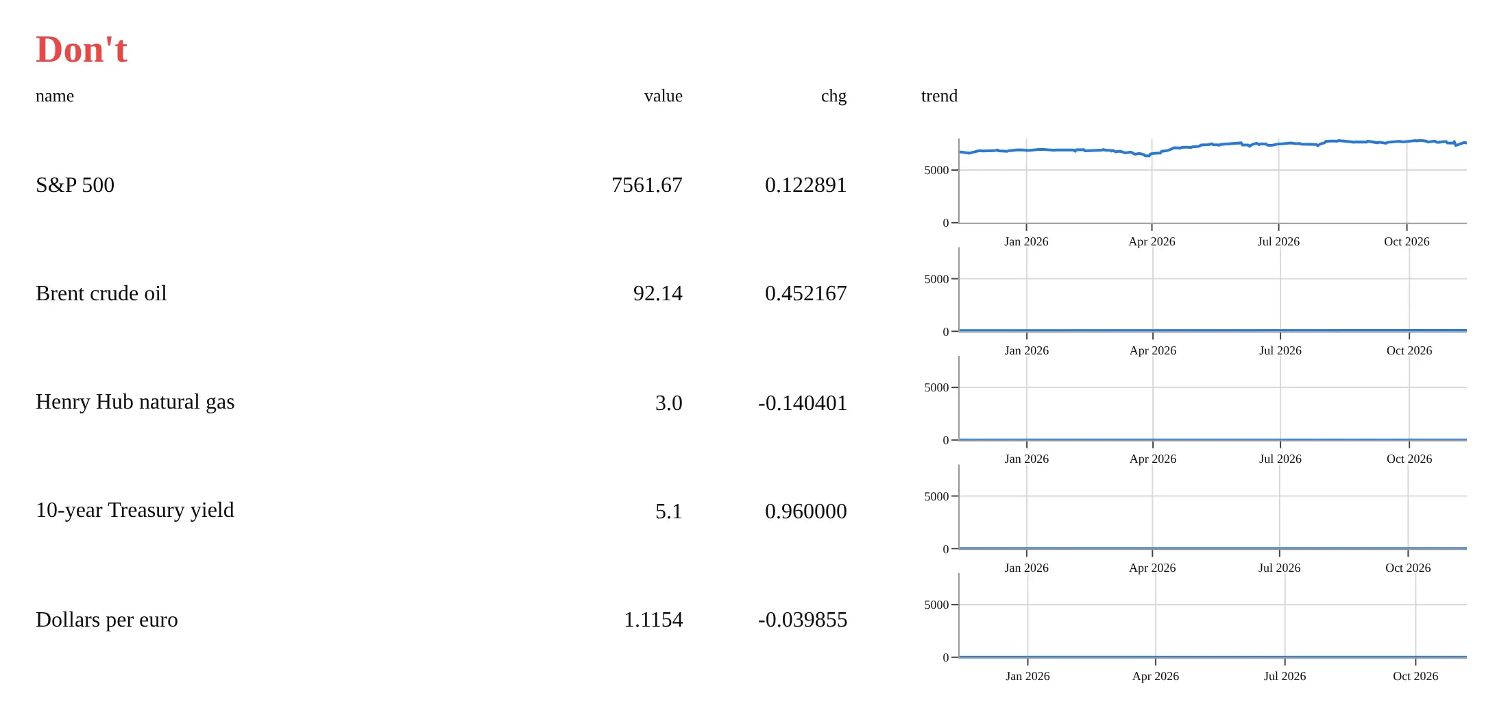
Do give each row its own y scale, hide the axes, format the numbers with separators and signed percents, align them to the right with units under the names, and put an orange dot on the latest day and gray dots on the low and high:
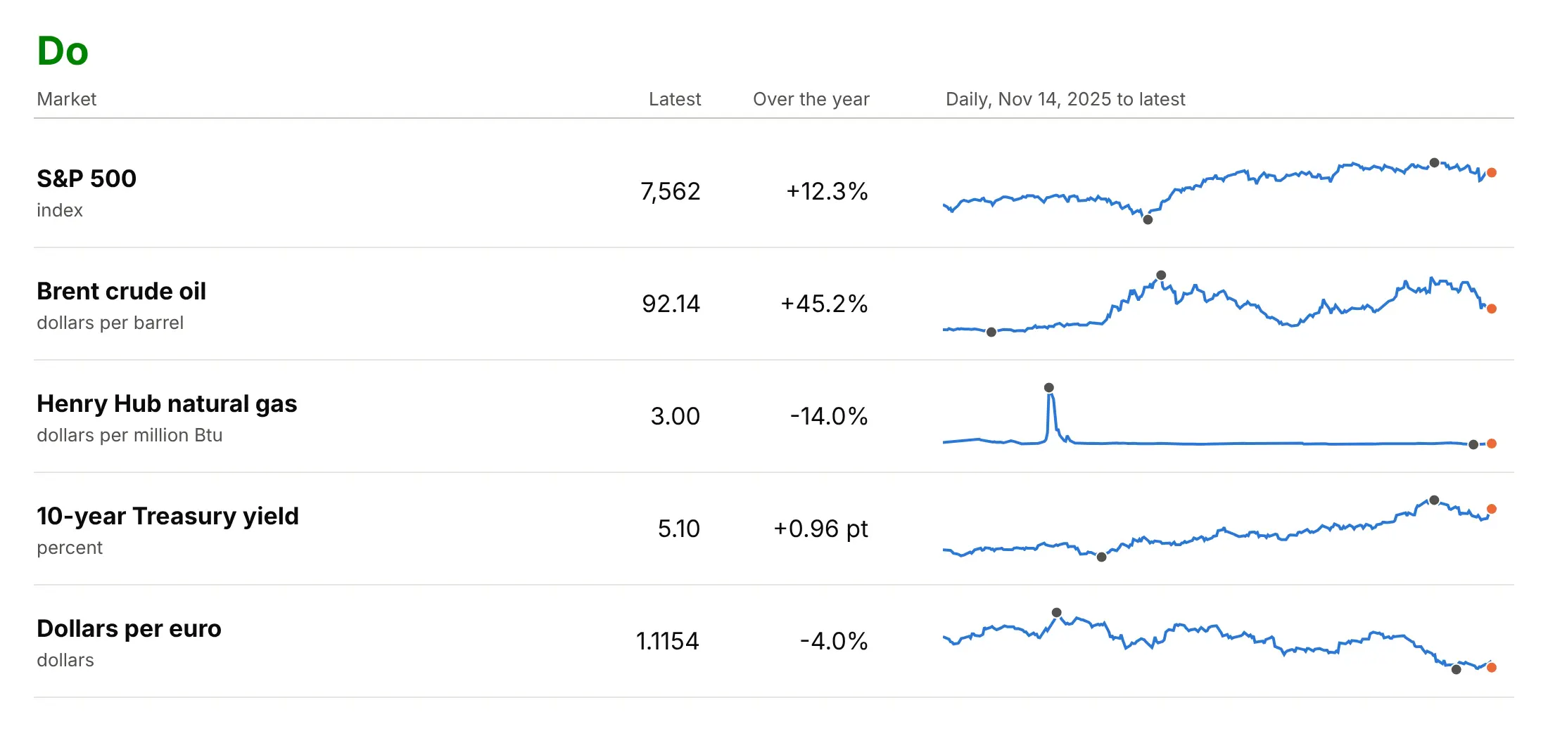
Checklist
Do
- Say what period and what frequency each sparkline covers, in the column header or the subtitle.
- Put the latest value as a number next to the sparkline, and mark it with a dot.
- Give rows with different units their own y scale, and rows with the same unit one shared scale.
- Mark the high and low, or a normal band, when readers will ask whether a value is unusual.
- Choose the aspect ratio so the typical slope is about 45 degrees, which is often between 4 and 20 times wider than tall.
- Use the same color for every line in a column, and a different one for the marks.
Don't
- Add axes, gridlines or legends to a sparkline. Move to a small multiples chart if readers need to look values up.
- Call a trend from a short line. A sparkline of 12 points shows noise as easily as a trend.
- Compare heights across rows with independent scales.
- Smooth the line, because the day-to-day wiggle is part of what a sparkline shows.
More sparkline examples
Seven more sparklines built from real public data, each with its source, the technique that makes it work and a prompt to rebuild it.
1. Temperatures on a shared scale
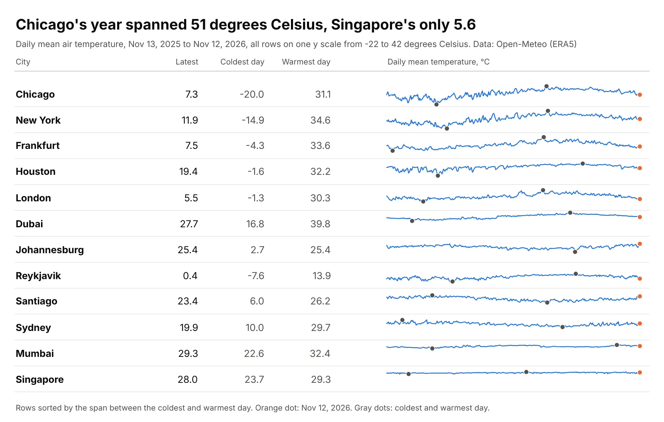
Chicago's daily mean temperature spanned 51.1 degrees Celsius over the year, from -20.0 on January 24, 2026 to 31.1 on July 1, while Singapore's spanned 5.6, and the shared scale is what makes that visible. Data: Open-Meteo Historical Weather API, which serves the ERA5 reanalysis (a gridded record of the weather built by the European Centre for Medium-Range Weather Forecasts from observations and a weather model).
Tip: write the coldest and warmest day as numbers in their own columns, and sort the rows by the span so the shared scale reads top to bottom.
Get the data from the Open-Meteo Historical Weather API (archive-api.open-meteo.com, daily temperature_2m_mean, ERA5) for Reykjavik, London, Frankfurt, New York, Chicago, Houston, Dubai, Mumbai, Singapore, Johannesburg, Sydney and Santiago, and shape it into a table (columns: city, date, tmean_c).Build a plotly sparkline table of the last 365 days, one shared y scale, sorted by the span between the coldest and warmest day, with the latest, coldest and warmest values in columns and gray dots on the extremes.
2. Monthly electricity generation by state
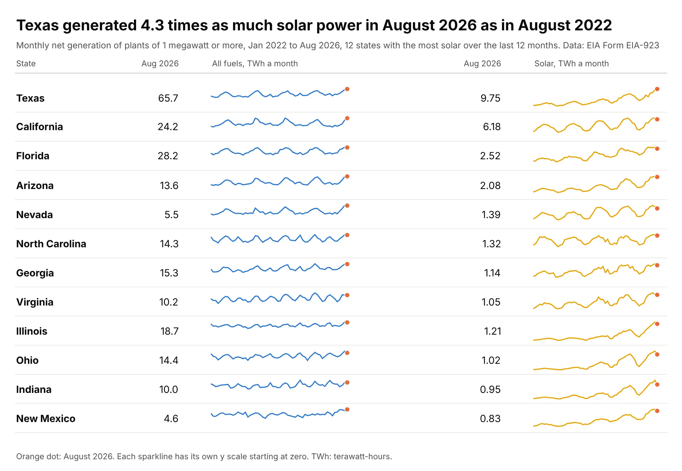
Texas generated 9.75 terawatt-hours (TWh) of solar power in August 2026, 4.3 times the 2.28 in August 2022, while its total of 65.7 TWh follows the seasons. Two sparklines per state, one for all fuels and one for solar, show the climb inside the seasonal wave. Data: EIA, Form EIA-923 monthly time series, plants of 1 megawatt or more (rooftop solar is not included).
Tip: start each y scale at zero so that a climb reads as growth and not as a wiggle.
Get the data from the US Energy Information Administration's Form EIA-923 monthly generation and fuel consumption time series (eia.gov/electricity/data/eia923, Page 1, files for 2022 to 2026, columns Plant State, Reported Fuel Type Code and Netgen January to December) and shape it into a table with one row per state and month (columns: state, month, all_gwh, solar_gwh).Build a plotly table of the 12 states with the most solar in the last 12 months, each with two sparklines (all fuels, solar) with y scales that start at zero and an orange dot on the latest month.
3. Sparklines inside KPI cards
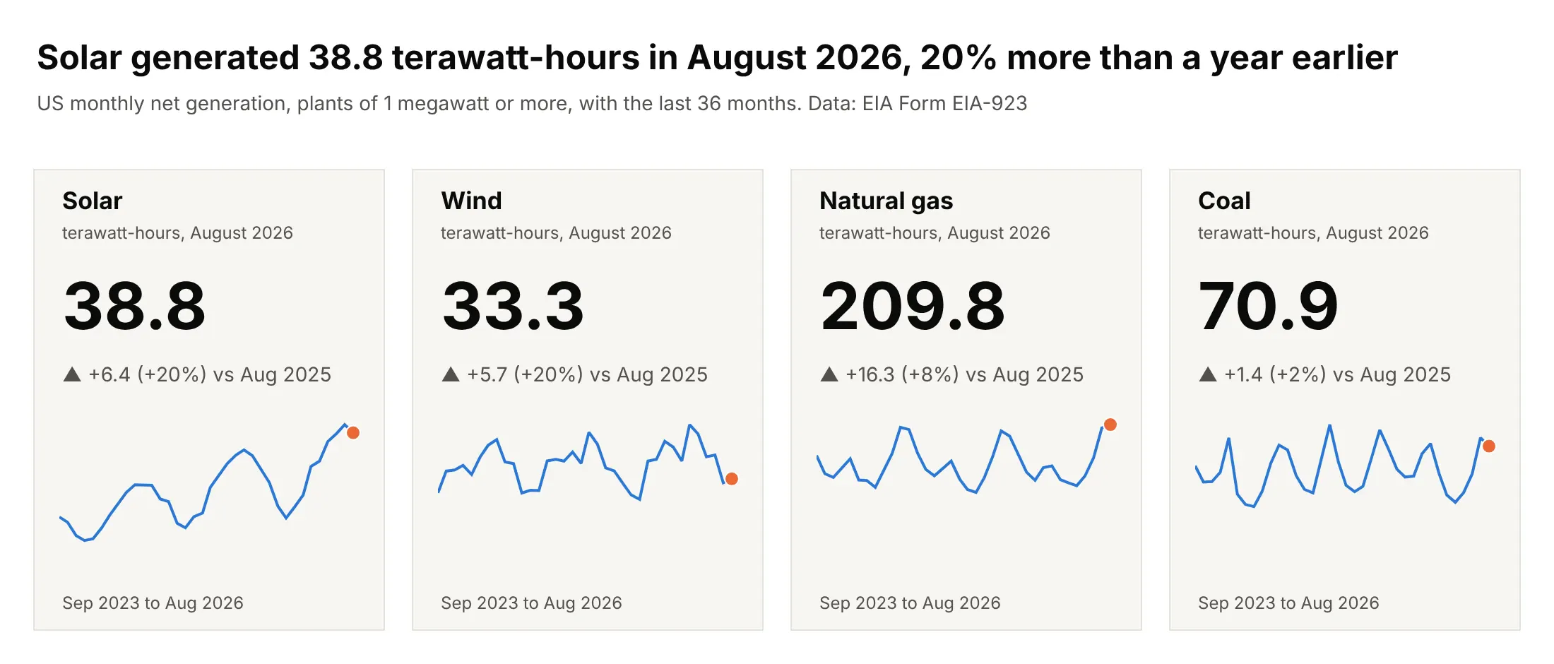
US utility-scale solar generated 38.8 TWh in August 2026, 20% more than a year earlier, and the sparkline on the card shows a climb in solar next to the seasonal waves of natural gas and coal. The delta compares with the same month a year before, because August against July would only show the season. Data: EIA, Form EIA-923, monthly net generation of the United States by fuel.
Tip: compare a monthly value with the same month of the year before, and say so in the delta's label.
Get the data from the US Energy Information Administration's Form EIA-923 monthly generation time series (eia.gov/electricity/data/eia923, Page 1, 2022 to August 2026) and shape it into a table (columns: fuel, month, gwh) for solar, wind, natural gas and coal for the whole United States.Build four plotly KPI cards with a big number for August 2026 in terawatt-hours, a gray delta against August 2025, and a 36-month sparkline with y starting at zero and an orange dot on August 2026.
4. Win/loss sparklines for 12 industries
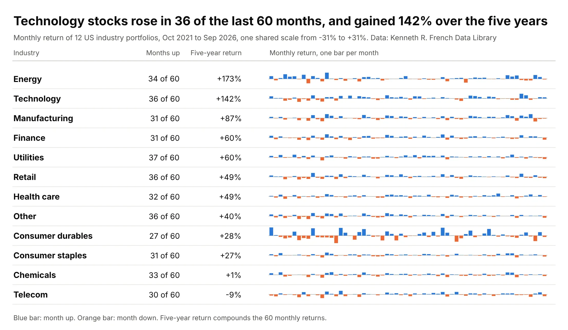
US technology stocks rose in 36 of the last 60 months and gained 142% over the five years, while energy gained 173% with only 34 up months, so the count of up months says little about the size of the gain. Bars above and below a zero line show both. Data: Kenneth R. French Data Library, 12 Industry Portfolios, value-weighted monthly returns.
Tip: use a go.Bar on a shared scale for returns, and color by sign instead of drawing the zero line heavily.
Get the data from Kenneth R. French's Data Library (mba.tuck.dartmouth.edu, 12_Industry_Portfolios_CSV.zip, "Average Value Weighted Returns -- Monthly", the last 60 months) and shape it into a table (columns: month, industry, ret in percent).Build a plotly table of the 12 industries with the count of up months, the compounded five-year return and a column sparkline of the 60 returns, blue for gains and orange for losses, one shared y scale.
5. A baseball season as a win/loss sparkline
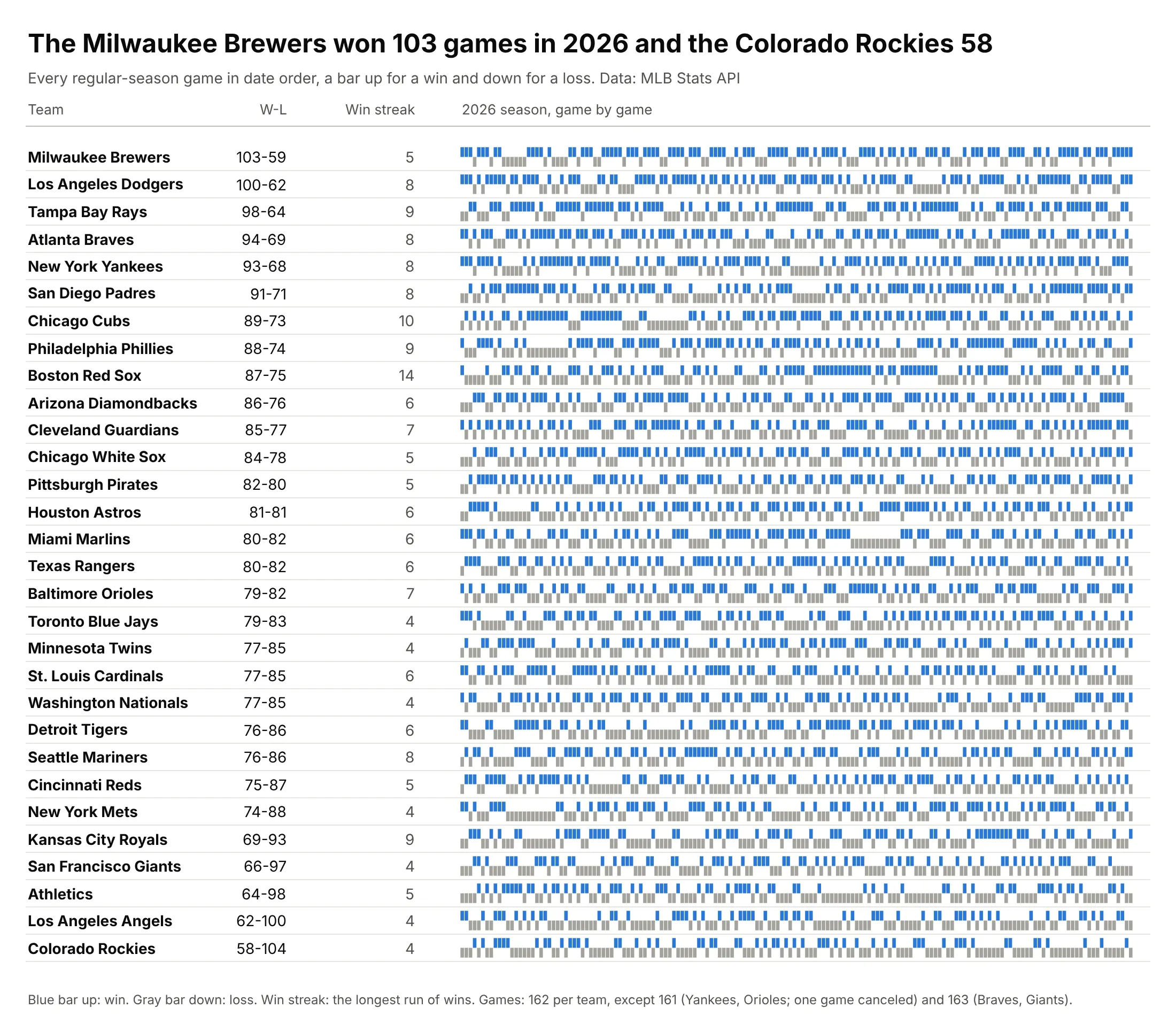
The Milwaukee Brewers won 103 of 162 games in 2026 and the Colorado Rockies 58, and the Boston Red Sox's 14-game win streak is a solid blue block in their row, which a record column hides. Tufte gave about 20 to 1 as the aspect ratio of a full baseball season, and these rows are 630 pixels wide and 20 tall, about 30 to 1. Data: Major League Baseball (MLB) Stats API, 2026 regular season.
Tip: put the record and the longest streak in numbers beside the bars, so readers can find the pattern in the row.
Get the data from the MLB Stats API (statsapi.mlb.com/api/v1/schedule, sportId 1, season 2026, gameType R, hydrate team) and shape it into a table with one row per team per game (columns: team, date, home, win, runs_for, runs_against).Build a plotly table of the 30 teams sorted by wins, each with its record, longest win streak and a win/loss sparkline of go.Bar (1 for a win in blue, -1 for a loss in gray).
6. Sunspots and the aspect ratio
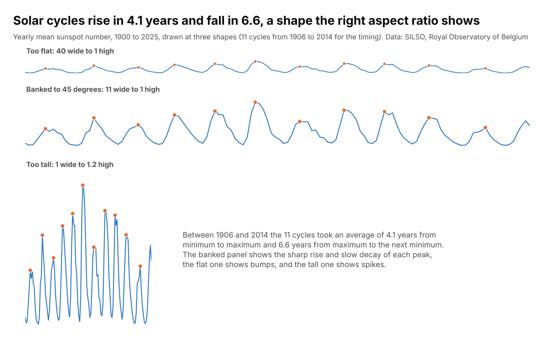
Between 1906 and 2014 the 11 solar cycles took an average of 4.1 years from minimum to maximum and 6.6 years to fall back, a lopsided shape that only appears when the aspect ratio is right. For these 126 yearly values, the ratio at which the typical slope is 45 degrees is 11 to 1, and the flatter and taller versions hide it. Tufte attributes this rule to the statistician William Cleveland, who found that people judge slopes best when they are near 45 degrees (the method is in Cleveland, McGill and McGill 1988). Data: SILSO (Sunspot Index and Long-term Solar Observations), Royal Observatory of Belgium, monthly mean total sunspot number V2.0, averaged by year.
Tip: compute the aspect ratio from the data as the y range divided by the x range times the median absolute slope, and set the sparkline's height to that times its width.
Get the data from SILSO (sidc.be/SILSO/DATA/SN_m_tot_V2.0.csv, monthly mean total sunspot number, semicolon-separated: year, month, decimal year, mean, standard deviation, observations, provisional flag) and shape it into a table with one row per year, 1900 to 2025 (columns: year, sunspots), as the mean of the monthly values.Build three plotly sparklines of the same series at 40:1, at the aspect ratio where the median absolute slope is 45 degrees, and at 1:1.2, with orange dots on the cycle peaks.
7. A sparkline inside a sentence
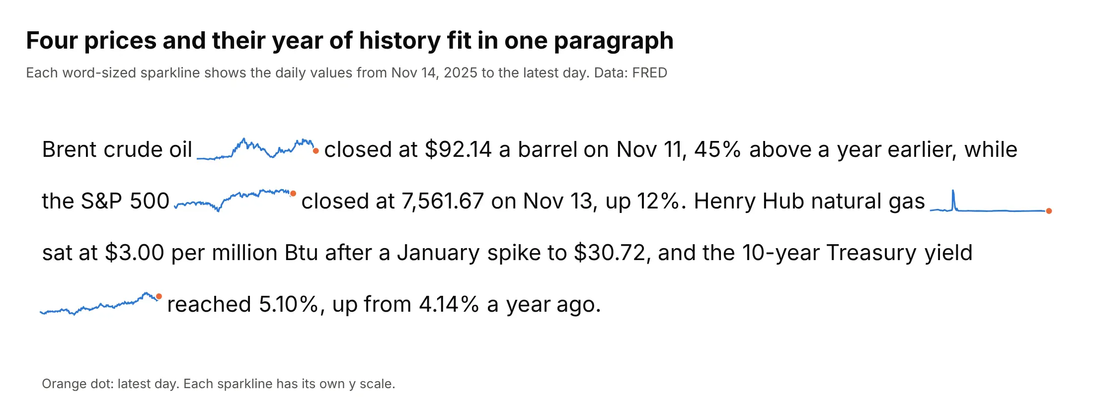
A sentence can carry its own charts: each sparkline sits right after the name of the series, is about as tall as the text, and ends in a dot on the latest day, which is the layout Tufte described as graphics "embedded in a context of words". Data: FRED, daily values from November 14, 2025 to the latest day.
Tip: make each sparkline about four words wide, and write the number that the sparkline illustrates right after it.
Get the data from FRED (fred.stlouisfed.org, series DCOILBRENTEU, SP500, DHHNGSP and DGS10, from 2025-11-14) and shape it into a table (columns: series, date, value).Build a plotly figure that lays out a four-sentence paragraph in Inter at 22 pixels, measuring each word with Pillow, with a word-sized sparkline (a go.Scatter on its own hidden axes, 120 pixels wide) after each series name and an orange dot on the latest day.
FAQ
Options to customize
A sparkline in Plotly is a go.Scatter or go.Bar trace with hidden axes, so these are the options that matter most. The full lists are in the scatter trace reference and the layout axes reference.
- xaxis.visible=False and yaxis.visible=False: hide every axis, tick and grid line, which is what makes a sparkline.
- layout.margin: set l, r, t and b to a few pixels so the line fills the figure, and leave room on the right for the marker on the last point.
- layout.width and layout.height: the aspect ratio, for example 240 by 48 for a sparkline in a table row.
- yaxis.range: the same range in every row for a shared scale, or a range from zero to the maximum for growth.
- go.Scatter(mode="lines", line=dict(width=2)): the line itself, drawn in one color for the whole column.
- A second go.Scatter(mode="markers") trace with cliponaxis=False: the dot on the last value, the high or the low.
- fill="tonexty" on two traces, the lower and the upper edge: a gray band for the normal range.
- line_shape="hv": a step line for values that change in jumps, such as a policy rate or a running count.
- go.Bar with marker.color per bar: column and win/loss sparklines.
- config={"staticPlot": True}: no hover or zoom, so a sparkline in a Dash table doesn't capture the mouse.