
Chris Parmer
November 18, 2026
Nyquist Plots - A Complete Guide
TL;DR
- A Nyquist plot draws how a system responds to sine waves of every frequency as one curve in the complex plane: the real part of the response on the x axis and the imaginary part on the y axis. Frequency runs along the curve instead of along an axis.
- Nyquist plots are also known as Nyquist diagrams and polar plots of the frequency response, and in impedance work as Cole-Cole plots. They are similar to Bode plots and Smith charts, which draw the same kind of response in other coordinates, and to scatter plots of complex numbers.
- Two fields use them with different conventions. Control engineers count how the curve circles the point -1 to tell whether a feedback loop is stable and to read its gain and phase margins. Electrochemists plot the real part of an impedance against minus its imaginary part on equal scales, and read the width of an arc as the resistance of a reaction, which is how electrochemical impedance spectroscopy (EIS) tracks the health of a battery.
- You can make a Nyquist plot with Plotly from one go.Scatter of real against imaginary part, with yaxis.scaleanchor="x" for equal scales; scipy.signal.freqresp computes the response from a transfer function. The code is below.
What is a Nyquist plot?
Nyquist plots look like this:
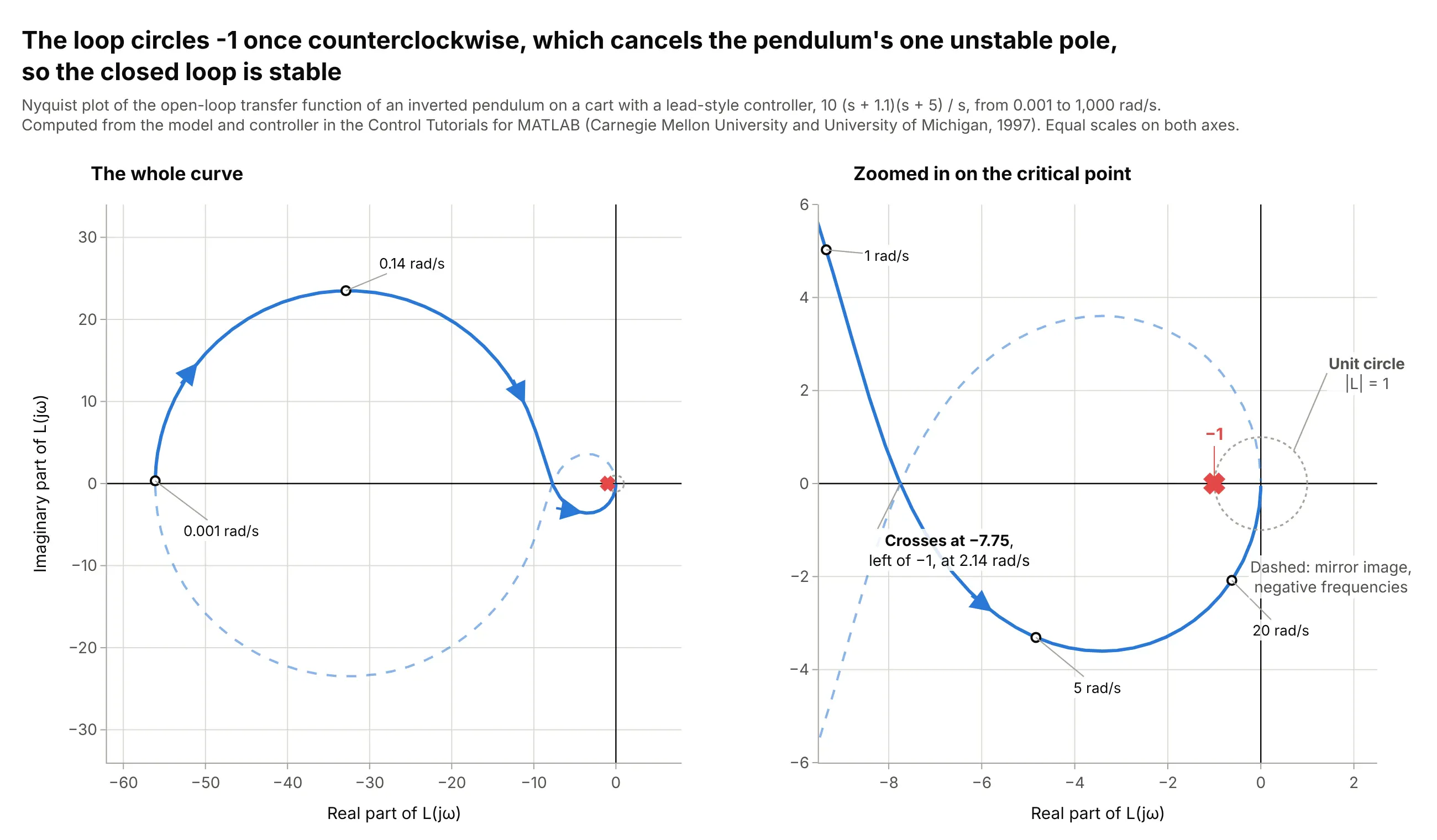
Data: computed from the inverted pendulum model and the controller in the Control Tutorials for MATLAB, a Carnegie Mellon University and University of Michigan teaching site (1997).
How do you read a Nyquist plot? In the example above, notice these things:
- Each point is one frequency of a sine wave going around a feedback loop. The distance from the origin says how much the loop amplifies that sine (its gain), and the angle from the positive real axis says how far the sine is shifted in time (its phase). The solid curve starts at 0.001 rad/s (radians per second) on the negative real axis at -56.1, swings up and around, and ends at the origin at high frequencies, where the loop passes almost nothing.
- The dashed curve is the mirror image across the real axis. It is the response to negative frequencies, which are not physical but complete the curve that the Nyquist criterion needs, and a closed Nyquist plot for a loop always includes it.
- The red x at -1 is the critical point. A sine wave sent around a loop with negative feedback comes back the same size and flipped when the gain is 1 and the phase is -180 degrees, which is the point -1, so it would keep going around forever. A curve that passes near -1 is a loop that nearly oscillates.
- A pendulum standing upright falls over, so this plant has one unstable pole (a built-in growth rate, here at +5.57 per second). The Nyquist criterion says the number of unstable poles of the closed loop is Z = N + P, where P is the unstable poles of the open loop and N is the number of clockwise circles around -1. Here P = 1 and the curve circles -1 once counterclockwise (N = -1), so Z = 0 and the closed loop is stable.
- The curve crosses the negative real axis at -7.75, at 2.14 rad/s, which is well to the left of -1. That means the gain could fall to 1/7.75, or 0.13 of its value (17.8 decibels, abbreviated dB), before the circle around -1 is lost; scaling the gain by 0.13 still gives a stable loop and 0.125 does not.
It's often used for charts like these:
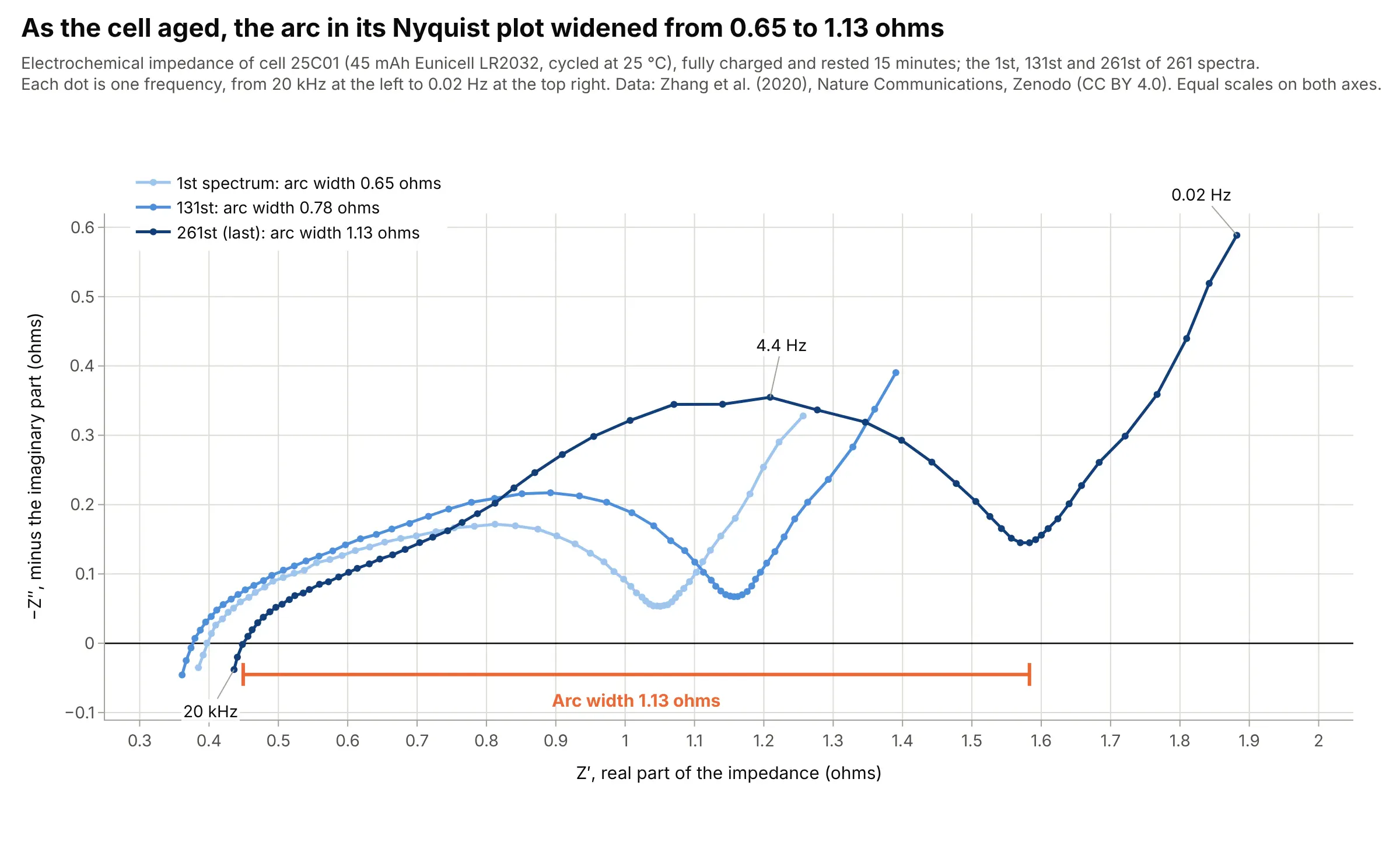
Batteries and fuel cells. The arc in a lithium-ion cell's impedance spectrum widened from 0.65 to 1.13 ohms over 261 measurements as the cell aged, which is why battery researchers use the Nyquist plot to follow degradation. Data: Zhang et al. (2020), Zenodo, CC BY 4.0, from the paper in Nature Communications.
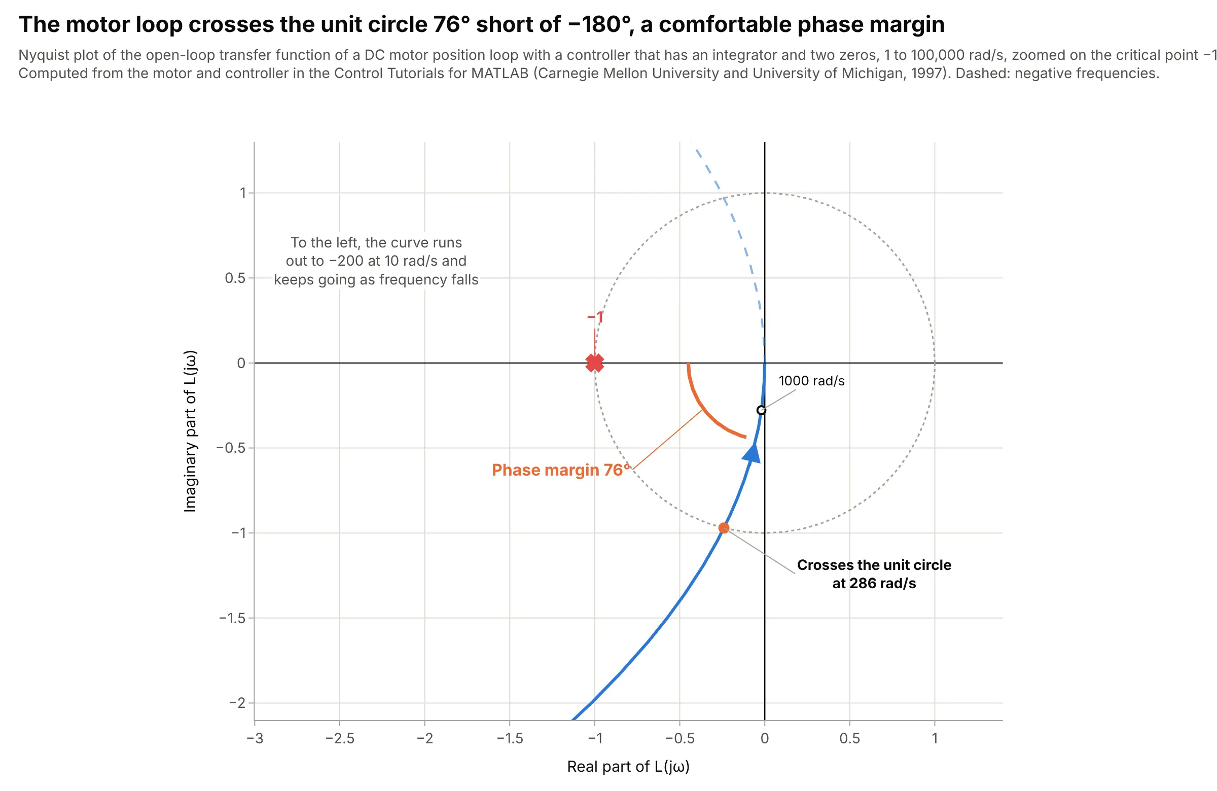
Motion control. The position loop of a DC motor with a controller crosses the unit circle at 286 rad/s with the curve 76 degrees short of the negative real axis, so its phase margin is 76 degrees; the curve never reaches the negative real axis, so the loop has no finite gain margin. Data: computed from the motor and controller in the Control Tutorials for MATLAB (Carnegie Mellon University and University of Michigan, 1997).
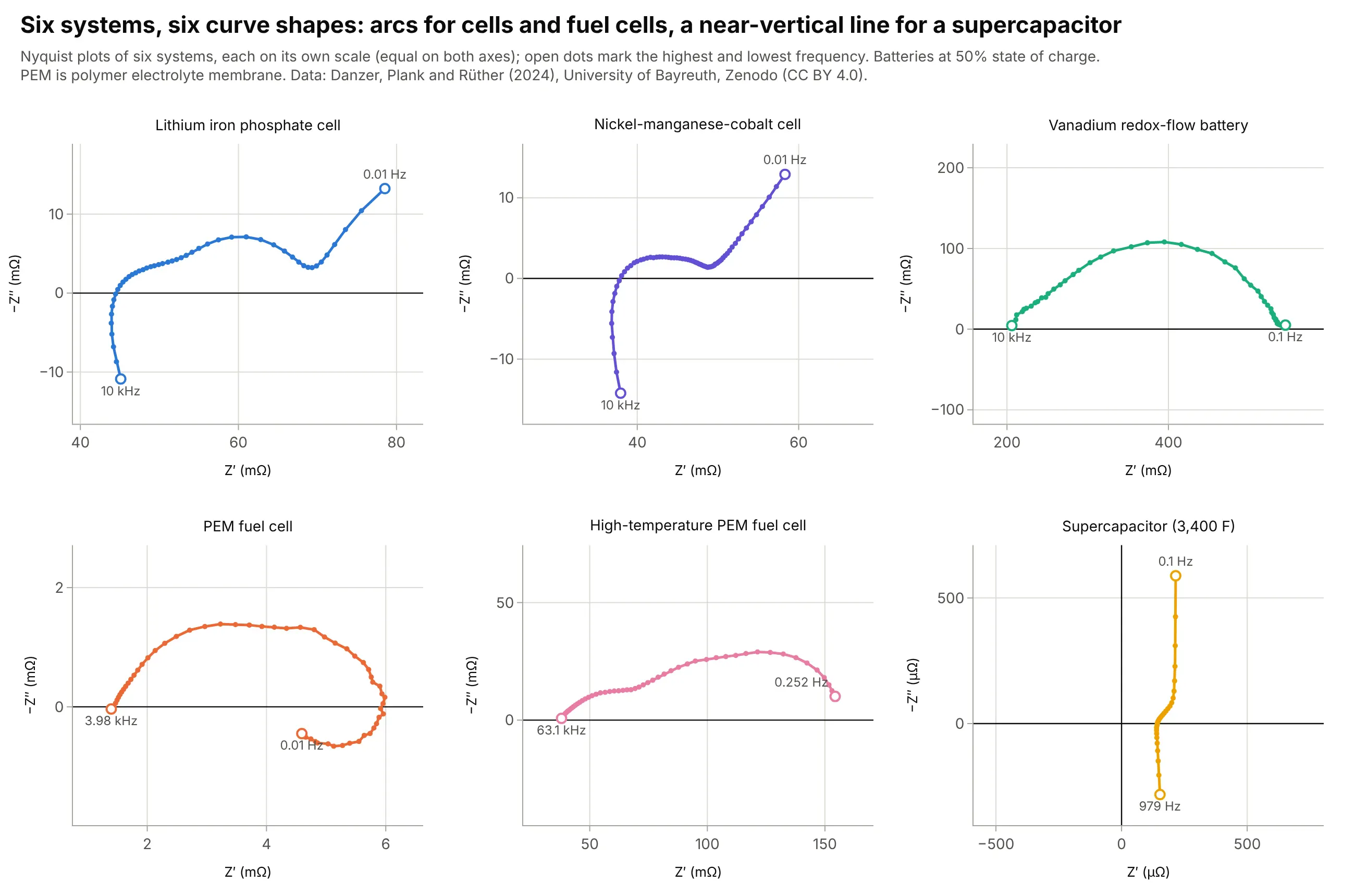
Comparing systems. Six systems measured in one lab give six shapes: the polymer electrolyte membrane (PEM) fuel cell's whole spectrum fits between 1.4 and 6.0 milliohms, while the vanadium redox-flow battery's single arc runs from 206 to 545 milliohms. Data: Danzer, Plank and Rüther (2024), Zenodo, University of Bayreuth, CC BY 4.0.
How to read a Nyquist plot
A Nyquist plot assumes three ideas that are second nature in control engineering and electrochemistry and unusual elsewhere: complex numbers, the frequency response, and a convention for what the axes mean in each field. Once those are clear, the shapes can be read directly.
Complex numbers in plain words
A complex number is a number with two parts, written 3 + 2j, where the first part (3) is called the real part and the second (2) the imaginary part, and j stands for the square root of -1 (mathematicians write i; engineers write j because i is the symbol for current). Two parts means the number is a point on a plane, with the real part along the x axis and the imaginary part along the y axis. The distance from the origin is the number's size, and the angle from the positive real axis is its phase:
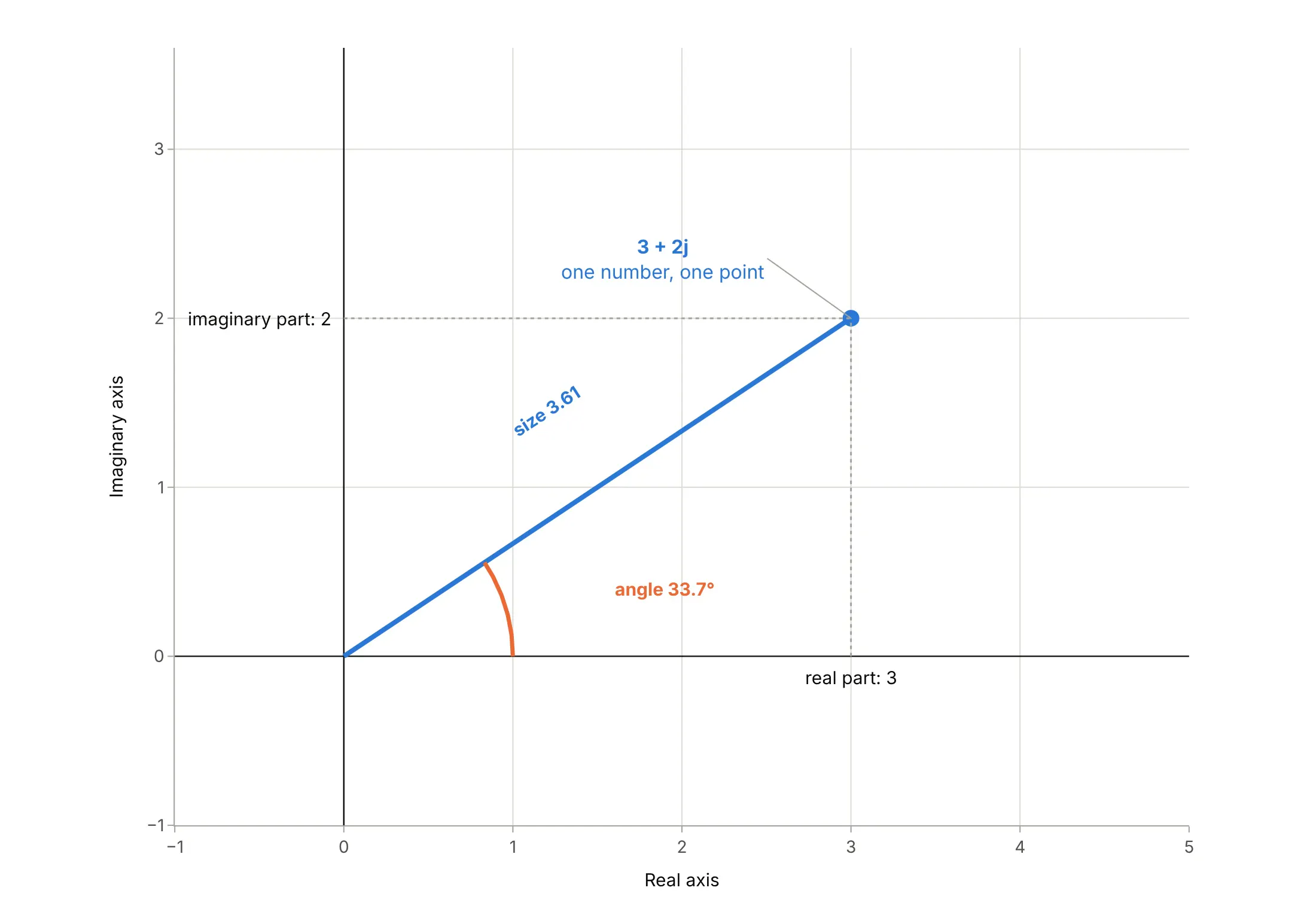
Data: a definition (not data).
Multiplying two complex numbers multiplies their sizes and adds their angles, which is why complex numbers describe things that scale and delay at the same time.
The frequency response: one complex number per frequency
Send a sine wave of one frequency into a system that is linear, such as a circuit, a battery, a motor or a loop with a controller. A sine wave of the same frequency comes out, with a different size and delayed by some fraction of a cycle. The frequency response is that pair of changes, written as one complex number: its size is the ratio of the output size to the input size, and its angle is the delay expressed as a phase. Sweep the frequency and the number traces a curve, and that curve is the Nyquist plot:
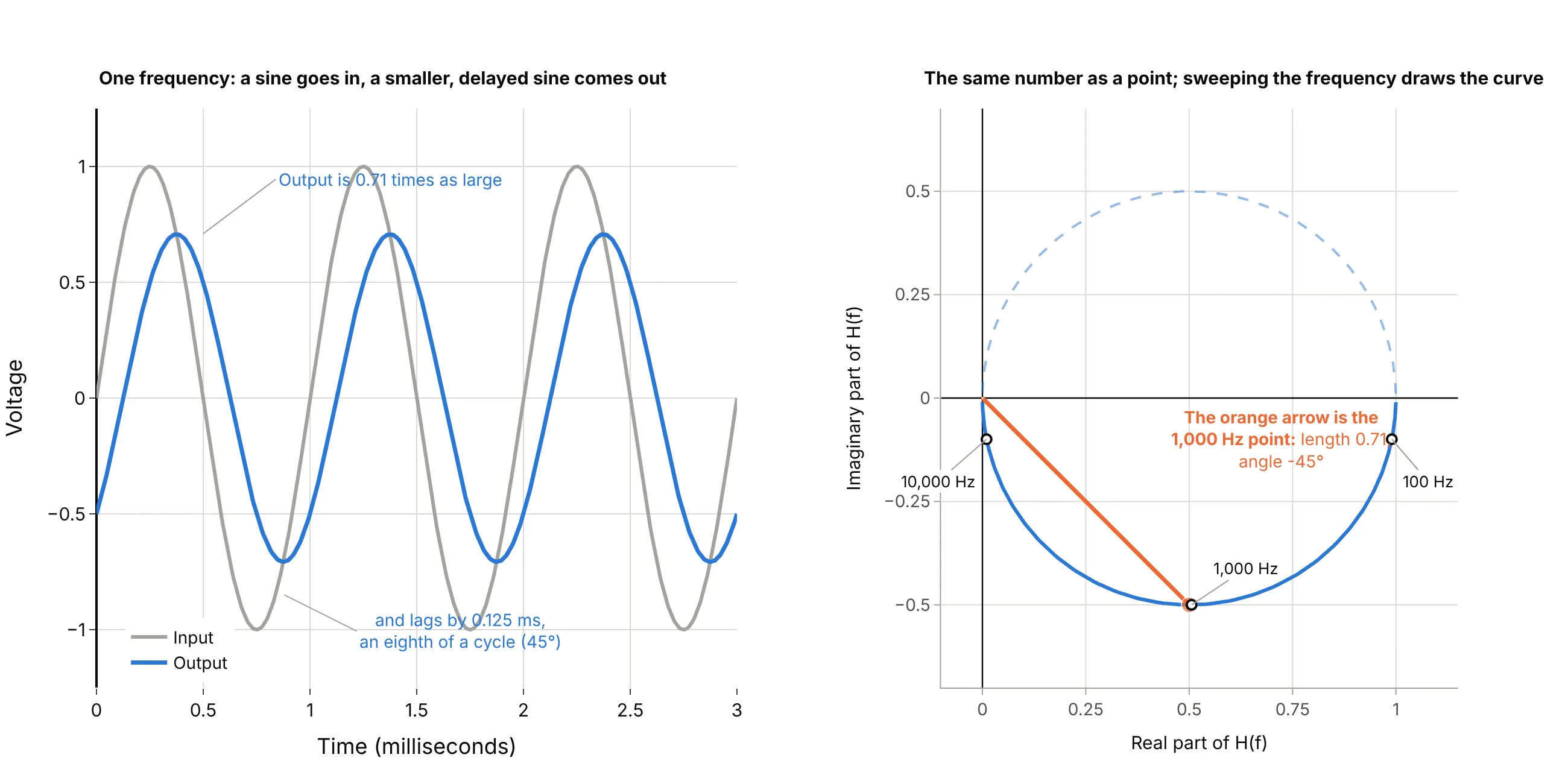
Data: computed from H(f) = 1 / (1 + j f / 1 kHz), not measured.
The Nyquist plot gives up the frequency axis to do this. Frequency is no longer a coordinate, so it has to be marked on the curve with labels or dots, as the examples here do.
Control engineering: the point -1, mirrored frequencies and margins
In control engineering the curve is the open-loop response L(jω), the response of everything around a feedback loop with the loop cut open, and ω (omega) is the angular frequency in radians per second. A loop with negative feedback oscillates at a frequency where L is exactly -1, so the plot's reference point is -1. Two parts of the convention surprise newcomers.
The first is the mirror image. The response at a negative frequency is the complex conjugate of the response at the matching positive frequency (the same real part and the opposite imaginary part), so the full curve is symmetric about the real axis. Software draws the positive half solid and the negative half dashed or faint, and the encirclement count uses the whole closed curve:
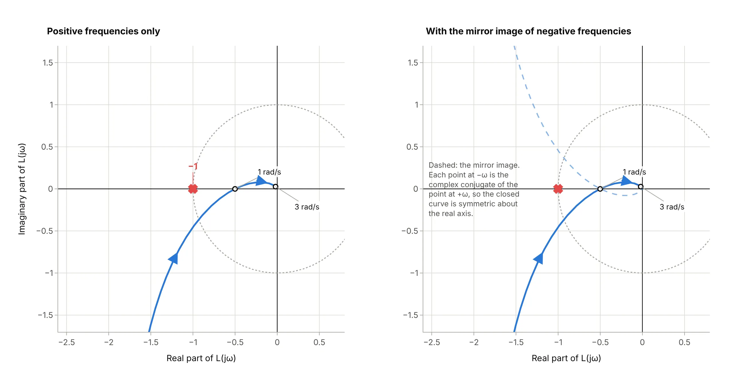
Data: computed from L(s) = 1 / (s³ + 2s² + s), the loop in our Bode plot guide, not measured.
The second is the margins. The stability criterion says what to count (clockwise circles around -1, plus the loop's unstable poles, must equal the unstable poles of the closed loop), and the distances from -1 say how much room there is. Where the curve crosses the negative real axis at a value of -0.5, the gain could double (a factor of 2, or 6.0 dB) before it reached -1: that is the gain margin. Where the curve crosses the unit circle, the distance in angle to the negative real axis is the phase margin:
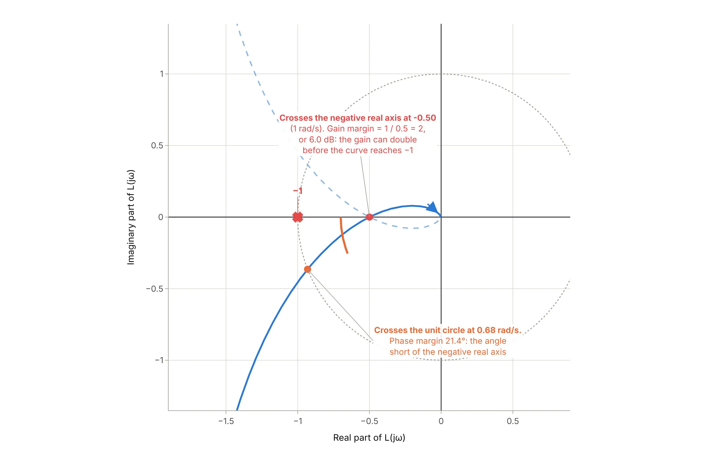
Data: computed from L(s) = 1 / (s³ + 2s² + s), not measured. The Bode plot guide reads the same 6.02 dB and 21.4 degrees from two panels.
A loop with an integrator (a pole at s = 0, as in the motor example) has an infinite response at zero frequency, so the curve starts infinitely far away; textbooks close it with a huge arc at infinity, and plots cut the picture off, as the motor example does.
Electrochemistry: Z′ against −Z″ on equal scales
Impedance is resistance for alternating current: the ratio of a voltage to a current at one frequency, written as a complex number Z = Z′ + jZ″. In electrochemical impedance spectroscopy (EIS), a small alternating current is passed through a cell at many frequencies, from kilohertz down to millihertz, and the impedance is measured at each. The convention differs from control engineering in three ways:
- The y axis is −Z″. A capacitor has a negative imaginary impedance, and cells are mostly capacitive, so plotting −Z″ turns the curve upward into the picture people expect. An inductor has a positive imaginary part, and so appears below the axis, as the 20 kHz end of the battery spectra does.
- The scales are equal. One ohm is the same length on both axes, so a semicircle looks like a semicircle and its width can be read in ohms. A stretched plot shows an ellipse and hides the shape that identifies the process.
- The shapes are read as circuit elements. The high-frequency crossing of the real axis is the series resistance. An arc is a resistance in parallel with a capacitance (for a battery, the charge-transfer reaction at an electrode surface), and its diameter on the real axis is that resistance. A rising line at low frequencies is diffusion, the slow movement of ions:
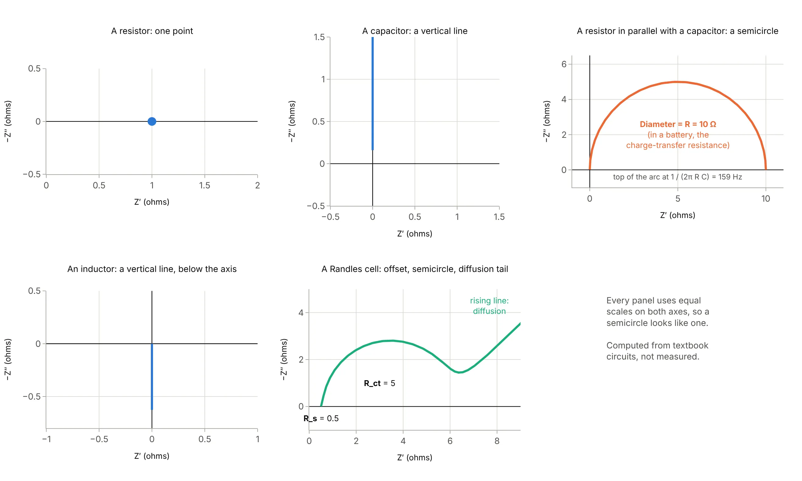
Data: computed from textbook circuits (a Randles cell with illustrative values), not measured. See the electrochemical impedance spectroscopy entry on Wikipedia for the semicircle's diameter and the apex frequency 1/(RC).
Real cells rarely give a clean semicircle: the arcs of several processes overlap and flatten, as in the battery examples below. For that reason this guide reads an arc's width straight off the plot, and calls it "arc width" rather than charge-transfer resistance, unless an equivalent circuit has been fitted.
Nyquist plots, Bode plots, and Smith charts
A Bode plot draws the same response as two stacked panels, magnitude and phase, against a log frequency axis, which keeps frequency visible and is easier to sketch. A Nyquist plot hides frequency but shows everything in one curve, and the encirclement rule works for loops that start unstable, which Bode margins cannot handle. A Smith chart is a Nyquist-like plot of a radio-frequency (RF) reflection coefficient with impedance circles drawn on top, and a polar chart draws the same complex numbers as a size and an angle instead of a real and imaginary part.
A short history
Harry Nyquist, an engineer at Bell Telephone Laboratories, published the criterion in "Regeneration Theory" in the Bell System Technical Journal in January 1932, to decide whether an amplifier with feedback would stay stable or run away into oscillation, which the paper calls carrying the feedback "beyond the singing point" (Nyquist 1932; scan on archive.org). The German engineer Felix Strecker had found the same result at Siemens in 1930, and Leroy MacColl and Hendrik Bode used an approach close to the textbook one in 1945 (Wikipedia). Nyquist's rule reads: "Plot plus and minus the imaginary part of AJ(iω) against the real part for all frequencies from 0 to ∞. If the point 1 + i0 lies completely outside this curve the system is stable; if not it is unstable." His point is +1, which matches a feedback ratio with the opposite sign to today's loop gain, whose critical point is -1.
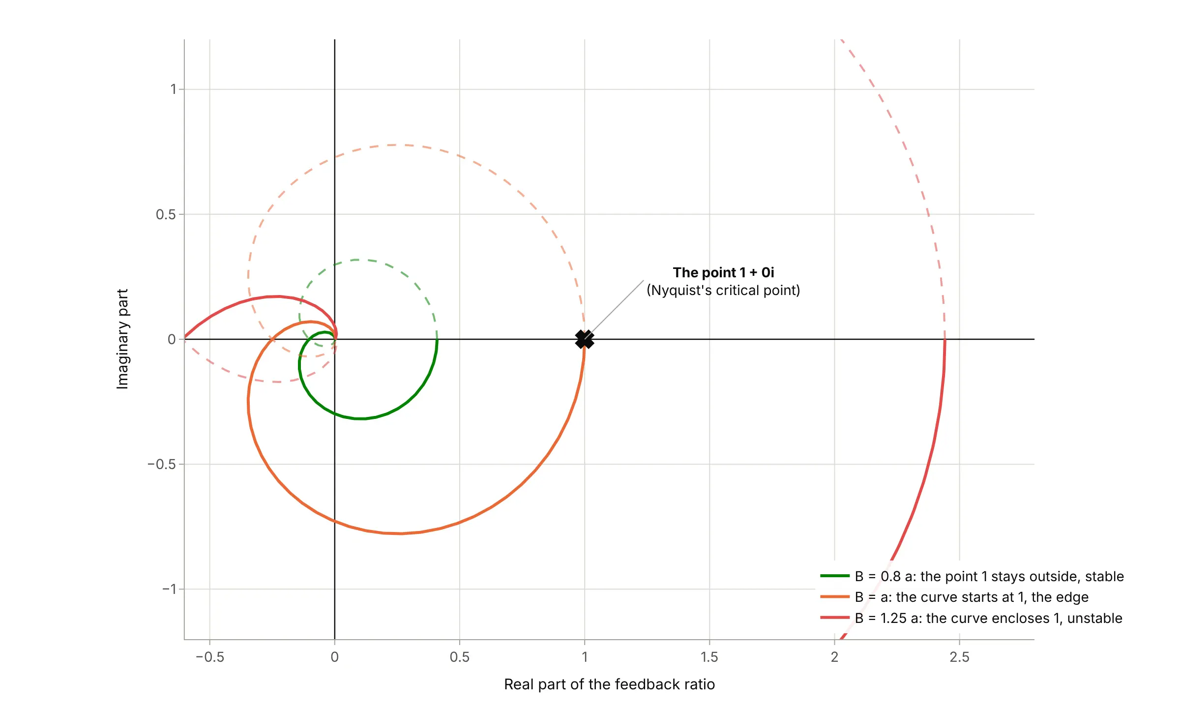
Data: computed from the formula in H. Nyquist, "Regeneration Theory", Bell System Technical Journal 11(1), 126-147, 1932 (his Example 5); this is a redraw with Plotly, not his figure.
The same plane came into electrochemistry and dielectric science separately. Cole and Cole plotted the imaginary against the real part of the dielectric response of materials in 1941 (Cole and Cole 1941), which is why impedance versions are still sometimes called Cole-Cole plots, and Randles published "Kinetics of rapid electrode reactions" in 1947, the standard citation for the equivalent circuit that carries his name (Randles 1947). Macdonald reviews the history of impedance spectroscopy in Electrochimica Acta.
Alternatives to a Nyquist plot
Here's the same lithium-ion cell spectrum (cell 25C01, the last of 261) drawn six ways. Some are better for the question, some worse, some just different:
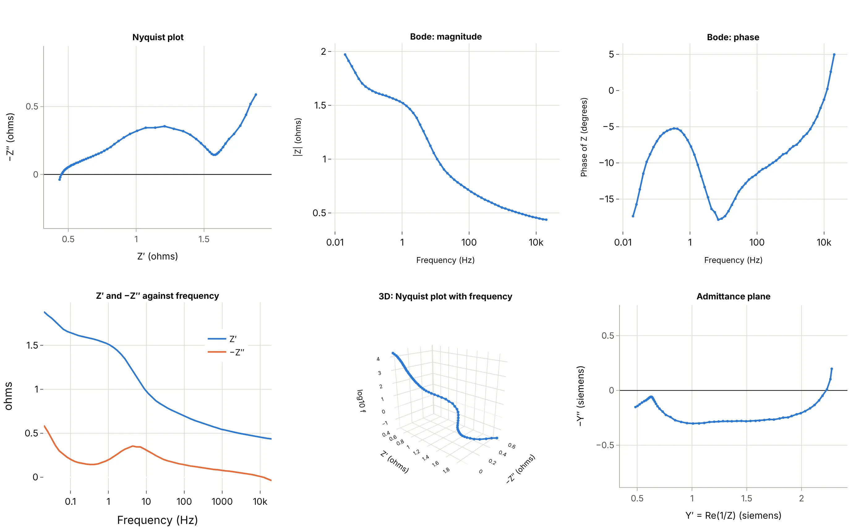
- Nyquist plot (better for seeing the processes). The arc, the valley and the diffusion tail are separate shapes, and the arc's width can be read in ohms, which none of the other views offers directly. Frequency is hidden, so label a few points.
- Bode plot (better for frequency). Magnitude and phase against log frequency show where each process happens, but the widths of the arcs are not visible. See the Bode plot guide.
- Real and imaginary parts against frequency (works too, for frequency). These two lines show frequency directly, but the shape of the arc and its width are harder to see.
- 3D curve (different). It keeps frequency as an axis, but numbers are hard to read off a 3D curve, and it needs interaction to be useful.
- Admittance plane (different). Plotting 1/Z turns parallel elements into sums, which helps fitting, but the arc loses its familiar shape and its width.
How to make a Nyquist plot
With AI
ChatGPT, Claude Code, GitHub Copilot, Cursor, and other AI tools are excellent at writing Plotly code. Name Plotly in the prompt, say whether the response comes from a transfer function or from measured impedance, and ask for equal scales:
Make a plotly Nyquist plot of the open-loop transfer functionL(s) = 10 (s + 1.1)(s + 5) / s * 4.5455 s / (s^3 + 0.1818 s^2 - 31.1818 s - 4.4545).- Compute L(jw) with scipy.signal.freqresp from 0.001 to 1000 rad/s.- Plot real part on x and imaginary part on y with go.Scatter, the mirror image for negative frequencies as a dashed line,the critical point -1 as a red x, and a dotted unit circle.- Set yaxis scaleanchor "x" so the scales are equal, and label a few frequencies on the curve.- Check: print where the curve crosses the negative real axis (about -7.75) and count the encirclements of -1.
With Plotly Studio
Plotly Studio is a product for creating data visualizations and Dash apps and for analyzing data with AI, available as a desktop app or embedded in Dash apps. Ask for a Nyquist plot the same way:
Show a Nyquist plot of this battery impedance file: Z' on x and -Z'' on y in ohms with equal scales, one curve per measurement colored from light to dark by cycle number, and a slider to pick the cycle.
In Python or JavaScript
This is the code AI tools write under the hood. You can make a Nyquist plot with Plotly from a go.Scatter of real against imaginary part, with yaxis.scaleanchor="x" so one unit is the same length on both axes. This helper returns a go.Figure, and every example in this guide builds on the same idea:
import numpy as npimport plotly.graph_objects as gofrom scipy import signaldef nyquist_plot(z, freq=None, name=None, color="#2a78d6", mirror=True):"""A Nyquist plot in Plotly: real part on x, imaginary part on y, equal scales, the critical point -1 marked."""fig = go.Figure()fig.add_trace(go.Scatter(x=z.real, y=z.imag, mode="lines", name=name, line=dict(color=color, width=3),customdata=freq, hovertemplate="%{customdata:.3g} rad/s: %{x:.3g} %{y:+.3g}j<extra></extra>"))if mirror: # negative frequencies are the complex conjugates, so the mirror image across the real axisfig.add_trace(go.Scatter(x=z.real, y=-z.imag, mode="lines", line=dict(color=color, width=2, dash="dash"),opacity=0.5, hoverinfo="skip", showlegend=False))fig.add_trace(go.Scatter(x=[-1], y=[0], mode="markers", name="-1", marker=dict(symbol="x", size=12, color="#e34948")))fig.update_layout(template="simple_white", xaxis_title="Real part", yaxis_title="Imaginary part", showlegend=False)fig.update_yaxes(scaleanchor="x", scaleratio=1) # equal scales: a circle looks like a circlereturn fig# The inverted pendulum with its controller (Control Tutorials for MATLAB): L(s) = 10 (s + 1.1)(s + 5) / s * P(s)num = [45.4545, 277.2727, 250.0]den = [1.0, 0.1818, -31.1818, -4.4545]w = np.logspace(-3, 3, 2000) # rad/s_, L = signal.freqresp(signal.TransferFunction(num, den), w)fig = nyquist_plot(L, freq=w)fig.update_xaxes(range=[-10, 2])fig.update_yaxes(range=[-6, 6])fig.show()
For measured impedance, pass z = re - 1j * minus_im and plot x=z.real, y=-z.imag (that is, Z′ and −Z″), and drop the mirror image and the critical point, which belong to control loops.
In JavaScript, plotly.js draws the same thing with three traces and the same scaleanchor:
<div id="chart"></div><script src="https://cdn.plot.ly/plotly-4.1.1.min.js"></script><script>// L(jw) = 1 / (jw (1 + jw)^2) at 600 frequencies from 0.05 to 100 rad/sconst w = Array.from({length: 600}, (_, i) => 10 ** (Math.log10(0.05) + (Math.log10(100) - Math.log10(0.05)) * i / 599));const re = [], im = [];for (const x of w) {const a = 1 - x * x, b = 2 * x; // (1 + jx)^2 = a + jbconst d = x * x * (a * a + b * b); // |jx (1 + jx)^2|^2re.push(-x * b / d); // real part of Lim.push(-x * a / d); // imaginary part of L}Plotly.newPlot("chart", [{x: re, y: im, mode: "lines", line: {color: "#2a78d6", width: 3}, name: "ω > 0"},{x: re, y: im.map(v => -v), mode: "lines", line: {color: "#2a78d6", width: 2, dash: "dash"}, opacity: 0.5, name: "ω < 0"},{x: [-1], y: [0], mode: "markers", marker: {symbol: "x", size: 12, color: "#e34948"}, name: "-1"}], {width: 800, height: 600,xaxis: {title: {text: "Real part"}, range: [-2.5, 0.5]},yaxis: {title: {text: "Imaginary part"}, scaleanchor: "x", scaleratio: 1, range: [-1.5, 1.5]}});</script>
Share it
Every Plotly chart has a Share chart button (the cloud icon in its toolbar) that uploads it to Plotly Cloud and gives you a link. Only you can see it until you change its visibility.
For a live app, put the chart in a Dash app and publish it with the Plotly Cloud CLI. Coding agents can run these commands for you:
pip install "dash[cloud]"plotly user loginplotly app publish
If your data has to stay in your own cloud or data center, publish to Dash Enterprise instead.
Dos and don'ts
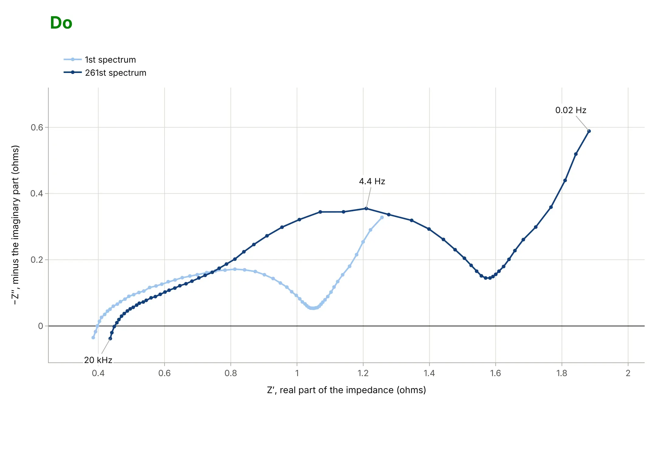
Most Nyquist plots that are hard to read break one of the conventions: equal scales, the sign of the imaginary axis, and labeled units. Here are two battery spectra drawn both ways, in the same two blues.
Don't plot the imaginary part without flipping its sign (the curve hangs below the axis), let the two axes take different scales so the arc stretches into a ridge, leave the axes named after column names such as re_ohm and im_ohm, show tick labels in scientific notation, use a serif font and a tinted background, and name the curves "trace 0" and "trace 1":
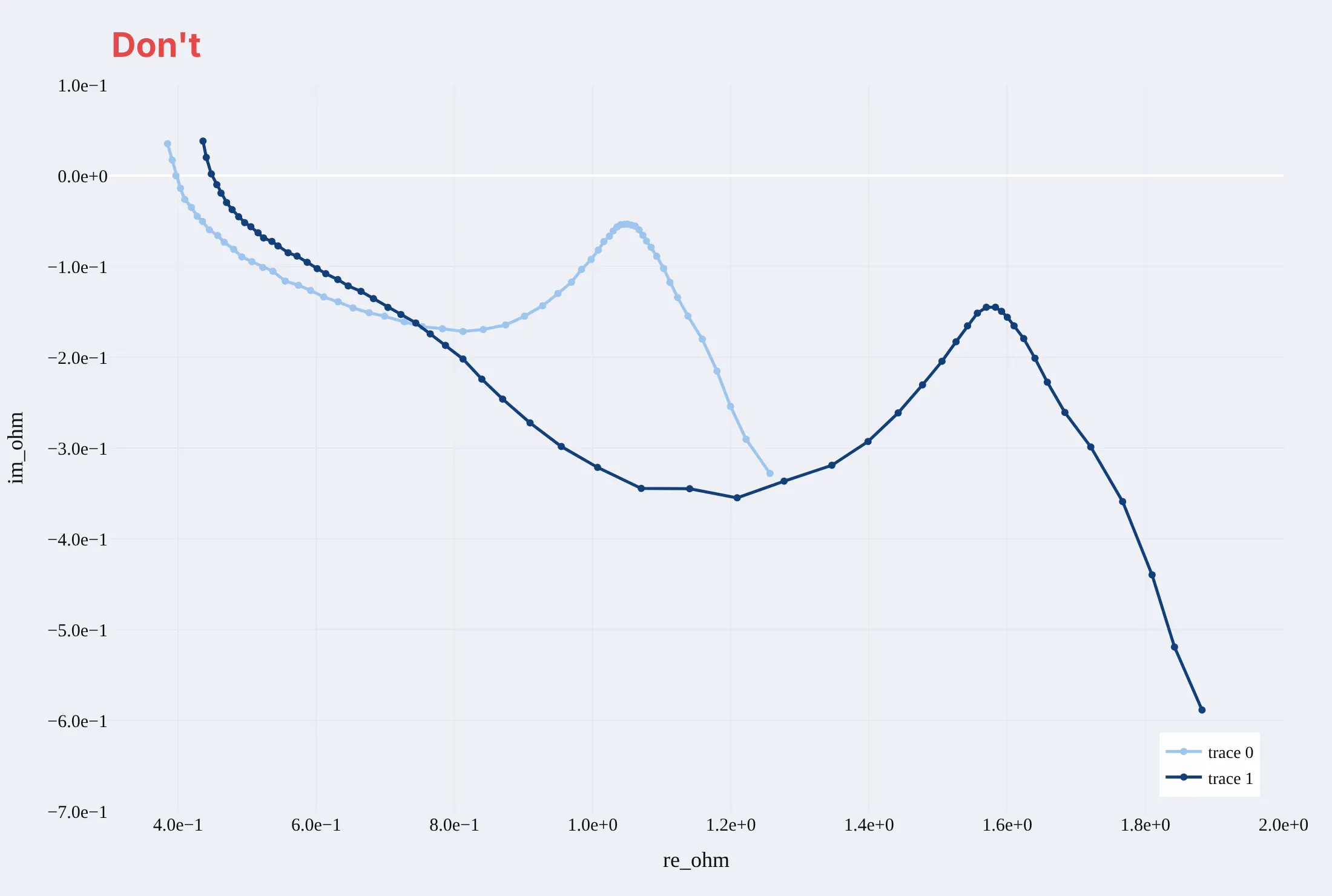
Do put −Z″ on the y axis so capacitive arcs point up, use equal scales on both axes, give each axis a name and a unit, mark a few frequencies along the curve, and name the curves for what they are:
Checklist
Do
- Use equal scales on both axes (yaxis.scaleanchor="x"), because a Nyquist plot is a picture of angles and distances.
- Label a few frequencies on the curve, since frequency is not an axis.
- For loops, draw the critical point -1, the unit circle, and the mirror image of negative frequencies, and say which direction counts as clockwise.
- For impedance, plot −Z″ upward and say so in the axis title, and state the frequency range and the direction of the sweep.
- Zoom on the region around -1 (or the arc) in a second panel when the curve extends far from it, and keep equal scales in the zoom.
Don't
- Stretch the plot to fill the space; the shape of an arc is the information.
- Draw a loop's Nyquist plot without saying whether it is the open loop; the criterion applies to the open loop.
- Read a semicircle's diameter as a charge-transfer resistance when two arcs overlap, without fitting a circuit.
- Compare spectra of different cells without removing the series resistance or saying so, since the arcs start at different points.
More Nyquist plot examples
Six more Nyquist plots, each with its source, the technique that makes it work, and a prompt to rebuild it. Five use measured data, and one is computed from a documented model.
1. 261 spectra of one battery
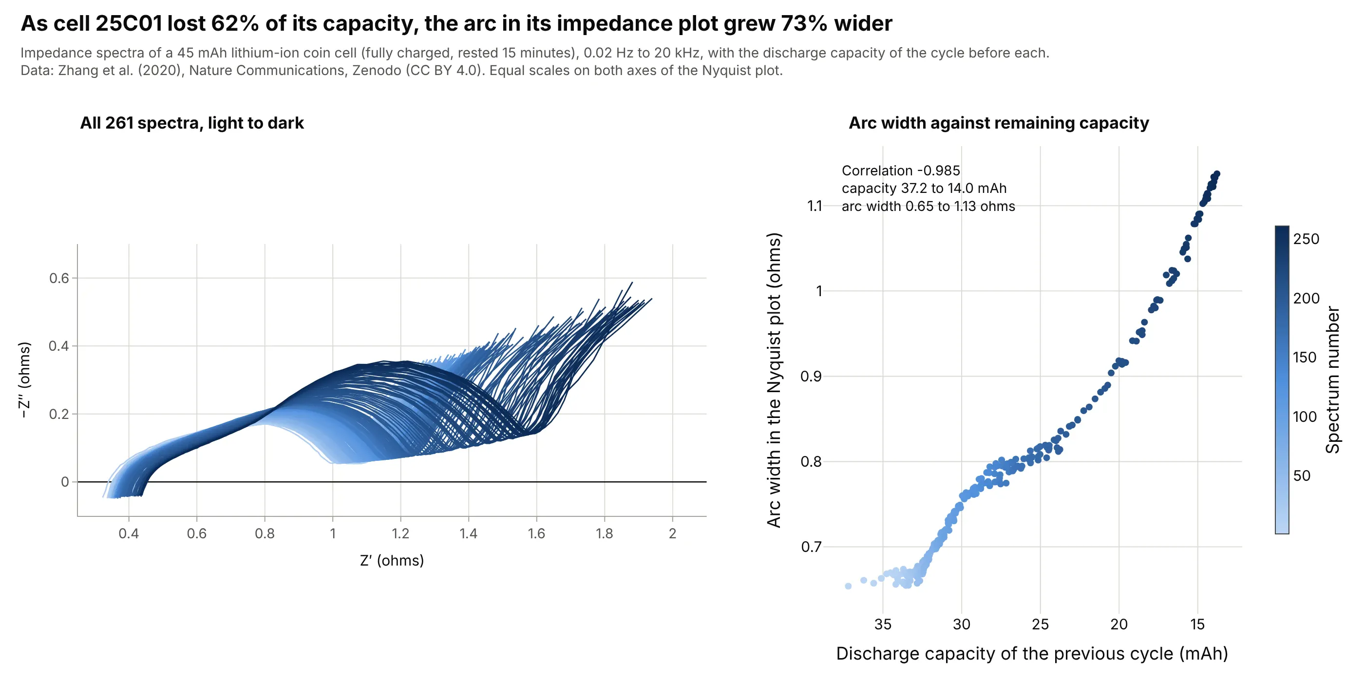
Cell 25C01 lost 62% of its discharge capacity (37.2 to 14.0 milliampere-hours, mAh) over 261 spectra while its arc width grew 73%, from 0.65 to 1.13 ohms, with a correlation of -0.985. Estimating how much of its original capacity a battery still holds, its state of health, from a quick impedance reading is the idea behind impedance-based diagnostics. Data: Zhang et al. (2020), Zenodo, CC BY 4.0. The capacity of each spectrum is the discharge capacity of the last finished cycle, matched by timestamp.
Tip: color every curve by its position in the sequence so a slow drift shows up as a gradient.
Get the data from the Zenodo record "Identifying degradation patterns of lithium ion batteries from impedance spectroscopy usingmachine learning" (doi 10.5281/zenodo.3633835, EIS data.zip, file EIS_state_V_25C01.txt: whitespace-separated, one header row,columns time/s, cycle number, freq/Hz, Re(Z)/Ohm, -Im(Z)/Ohm, |Z|/Ohm, Phase(Z)/deg; 261 spectra of 60 frequencies).Make a plotly Nyquist plot with Z' on x and -Z'' on y, one thin line per cycle number colored from light to dark blue,equal scales (yaxis scaleanchor "x"), and a slider that highlights one cycle.
2. Twelve cells, and where the arc stops telling the story
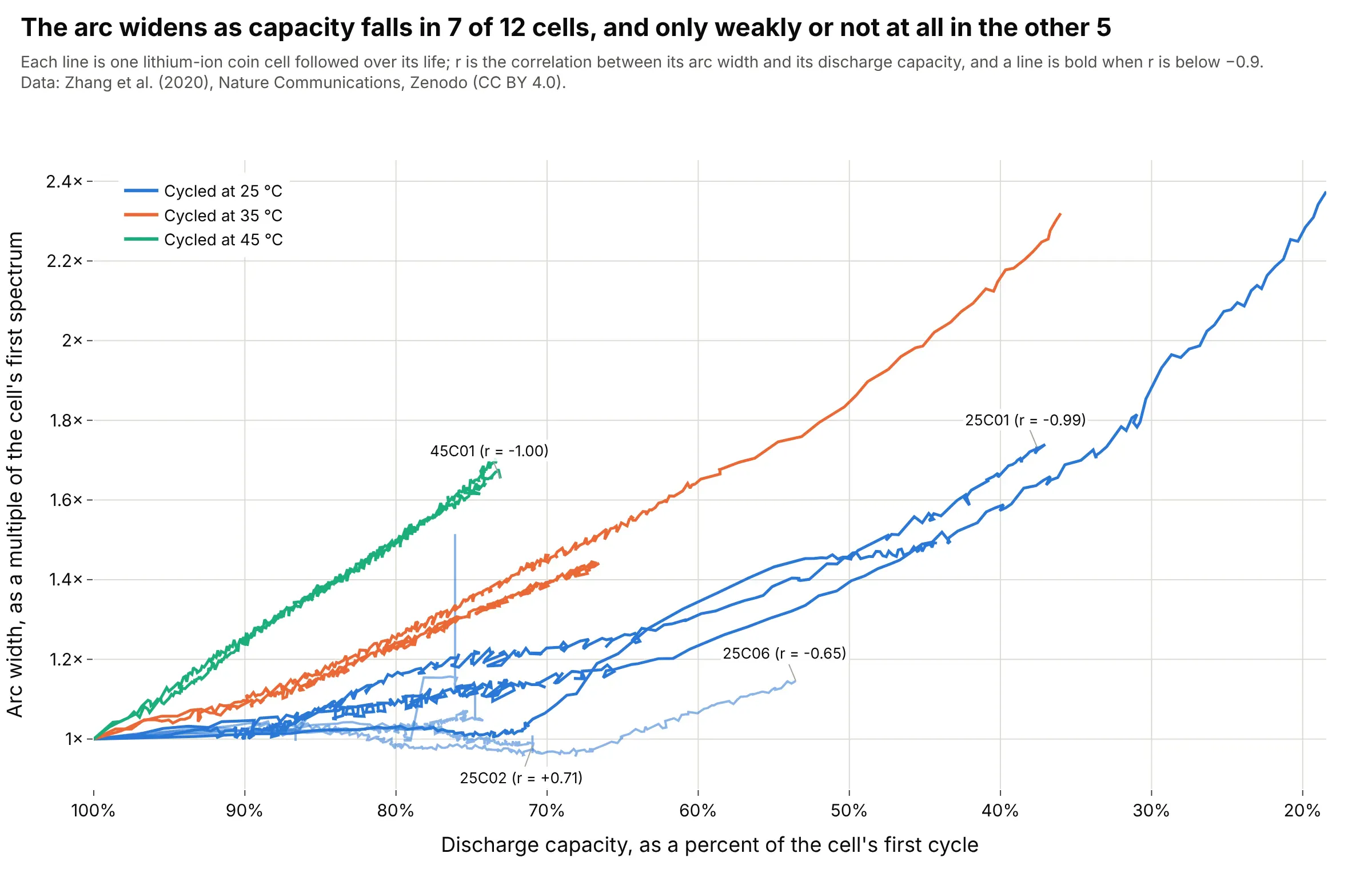
The arc width tracks capacity loss closely in 7 of 12 cells (correlation below -0.9) and only loosely in the rest: cell 25C02's arc stayed at 1.12 to 1.10 ohms while its capacity fell from 35.1 to 24.9 mAh, a 29% loss. A health indicator read off a Nyquist plot has to be checked on each cell design before it is trusted. Data: Zhang et al. (2020), Zenodo, CC BY 4.0, 12 cells at 25, 35 and 45 °C.
Tip: give the cells where the rule breaks a label, so the reader sees the exceptions instead of an average.
Get the data from the Zenodo record doi 10.5281/zenodo.3633835 (EIS data.zip: EIS_state_V_<cell>.txt for 12 cells, columnstime/s, cycle number, freq/Hz, Re(Z)/Ohm, -Im(Z)/Ohm, |Z|/Ohm, Phase(Z)/deg; Capacity data.zip: Data_Capacity_<cell>.txt, lastcolumn Capacity/mA.h, ox/red = 0 for discharge). For each spectrum, read the arc width as the real part at the lowest -Z''between 3 Hz and 0.1 Hz minus the real part where -Z'' crosses zero at high frequency, and match it to the discharge capacity ofthe last cycle that ended before the spectrum's timestamp.Make a plotly line chart, one line per cell, arc width relative to the first spectrum against capacity relative to the first cycle(reversed x axis), colored by cell temperature, and label the cells with the weakest correlation.
3. Warmer cells, narrower arcs
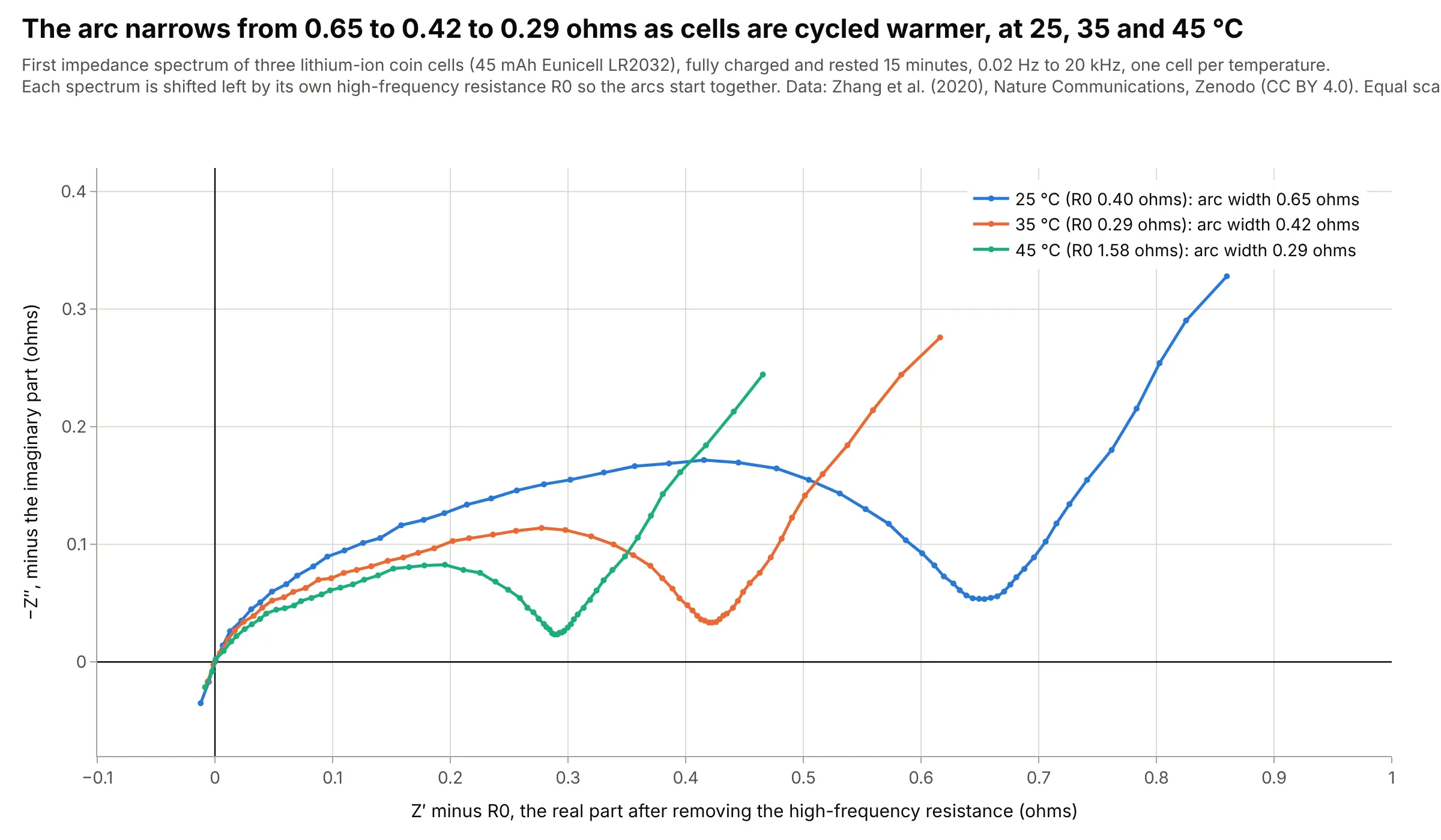
The first spectrum of a cell cycled at 45 °C has an arc 0.29 ohms wide against 0.42 ohms at 35 °C and 0.65 ohms at 25 °C. Across all twelve cells the order holds: the two 35 °C cells start at 0.42 ohms and the two 45 °C cells at 0.29, while the eight 25 °C cells start between 0.63 and 1.26 ohms. Each spectrum is shifted left by its own high-frequency resistance, because 45C01's first spectrum starts at 1.58 ohms against 0.27 to 0.56 for the others. Data: Zhang et al. (2020), Zenodo, CC BY 4.0. The cell names carry the cycling temperature.
Tip: when curves start at different offsets, subtract the offset and say so on the axis, so the arcs can be compared.
Get the data from the Zenodo record doi 10.5281/zenodo.3633835 (EIS data.zip: EIS_state_V_25C01.txt, EIS_state_V_35C01.txt,EIS_state_V_45C01.txt; columns time/s, cycle number, freq/Hz, Re(Z)/Ohm, -Im(Z)/Ohm, |Z|/Ohm, Phase(Z)/deg; use cycle number 1).Make a plotly Nyquist plot of the three first spectra with Z' minus the high-frequency intercept on x and -Z'' on y, equal scales,one color per temperature (25, 35, 45 C), and the arc width in each legend entry.
4. A resonance is a circle
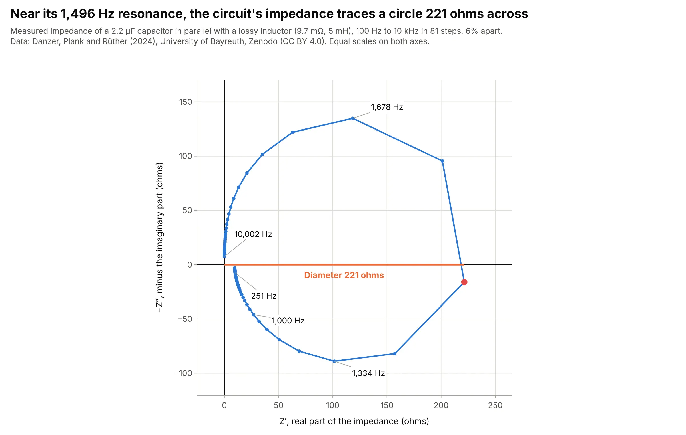
A capacitor in parallel with an inductor that has a little resistance has an impedance that peaks at its resonance and sweeps a circle in the Nyquist plane: the measured circuit reached 221 ohms at 1,496 Hz, close to the 1,517 Hz that its nominal 5 mH and 2.2 µF give. The circle's diameter on the real axis is the impedance at resonance, and mechanical structures and antennas show the same circles. Data: Danzer, Plank and Rüther (2024), Zenodo, CC BY 4.0, file rlc_circuit.json (81 frequencies, 6% apart, so only about a dozen points fall on the circle).
Tip: draw the straight lines between measured points rather than a smooth curve, so the reader sees how densely the circle was sampled.
Get the data from the Zenodo record doi 10.5281/zenodo.10794584 (file rlc_circuit.json: a JSON object with keys f in Hz,z_real and z_imag in ohms, 81 frequencies from 100 Hz to 10 kHz).Make a plotly Nyquist plot with z_real on x and -z_imag on y with equal scales (yaxis scaleanchor "x"), markers on the line,the largest real part marked with a dot and a line from the origin to it labeled with its value, and frequencies labeled at four points.
5. Six controllers for one pendulum
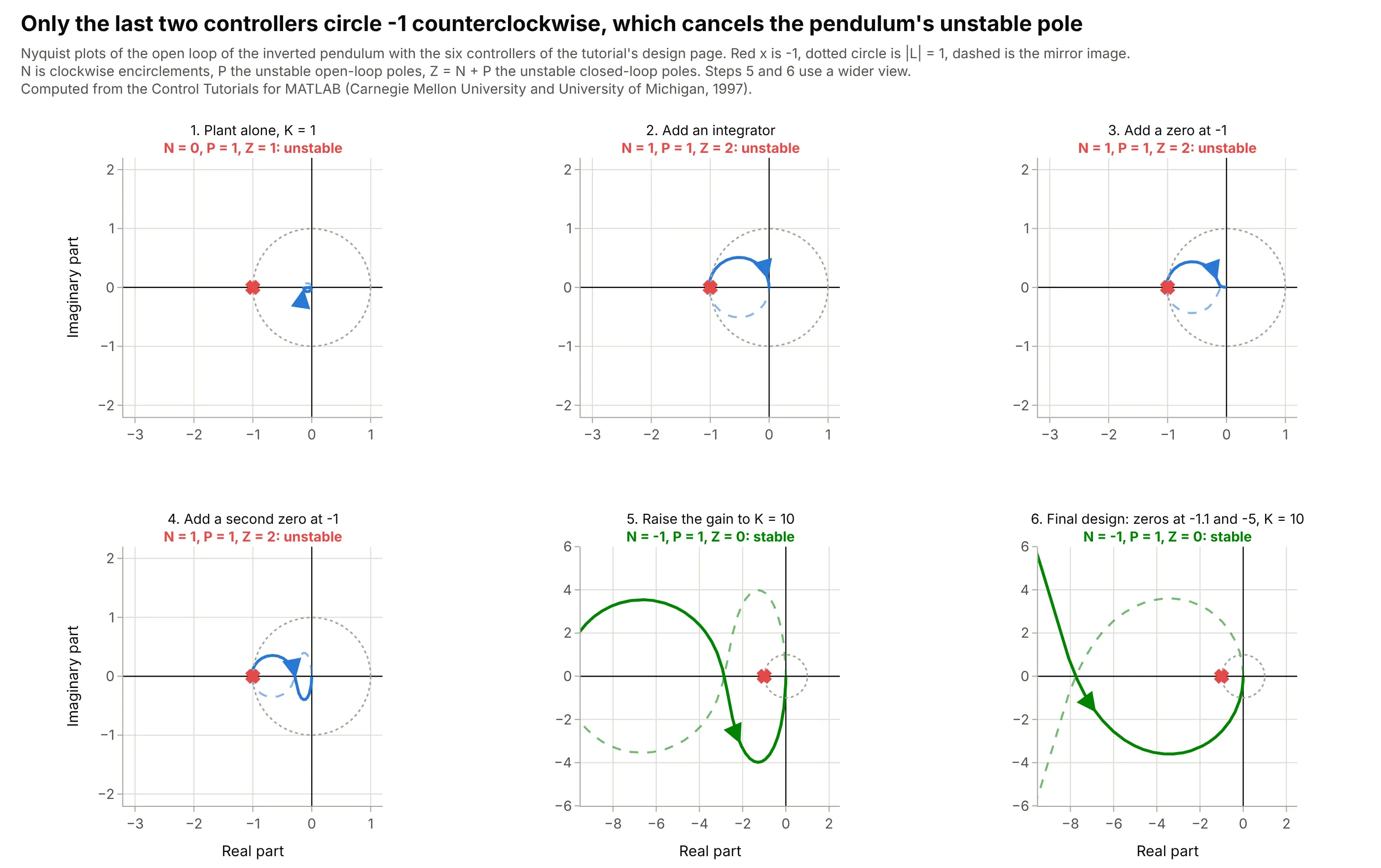
The tutorial adds a controller piece by piece, and the Nyquist plot says why each step fails until the gain is high enough: with the plant alone, N = 0 and P = 1, so Z = 1 and the loop is unstable; an integrator and two zeros leave it at Z = 2; raising the gain to 10 pushes the curve past -1 (it crosses the real axis at -2.85) and gives N = -1, Z = 0. The encirclement count agrees with the closed-loop poles in every case. Data: computed from the model and the six controllers in the Control Tutorials for MATLAB (Carnegie Mellon University and University of Michigan, 1997).
Tip: put N, P and Z in each panel title, so the reader can check the rule themselves.
Use this model of an inverted pendulum on a cart: M = 0.5, m = 0.2, b = 0.1, I = 0.006, l = 0.3, g = 9.8,q = (M+m)(I+m l^2) - (m l)^2, P(s) = (m l / q) s / (s^3 + b (I + m l^2) / q s^2 - (M+m) m g l / q s - b m g l / q).Make a plotly figure with 2 rows of 3 Nyquist plots for the loops K C(s) P(s) with C = 1, 1/s, (s+1)/s, (s+1)^2/s, then K = 10 with (s+1)^2/s,and K = 10 with (s+1.1)(s+5)/s. Mark -1, draw the unit circle, count the clockwise encirclements N numerically, and show N, P and Z = N + P ineach panel title. Equal scales (yaxis scaleanchor "x") in every panel.
6. A measured filter spirals into the origin
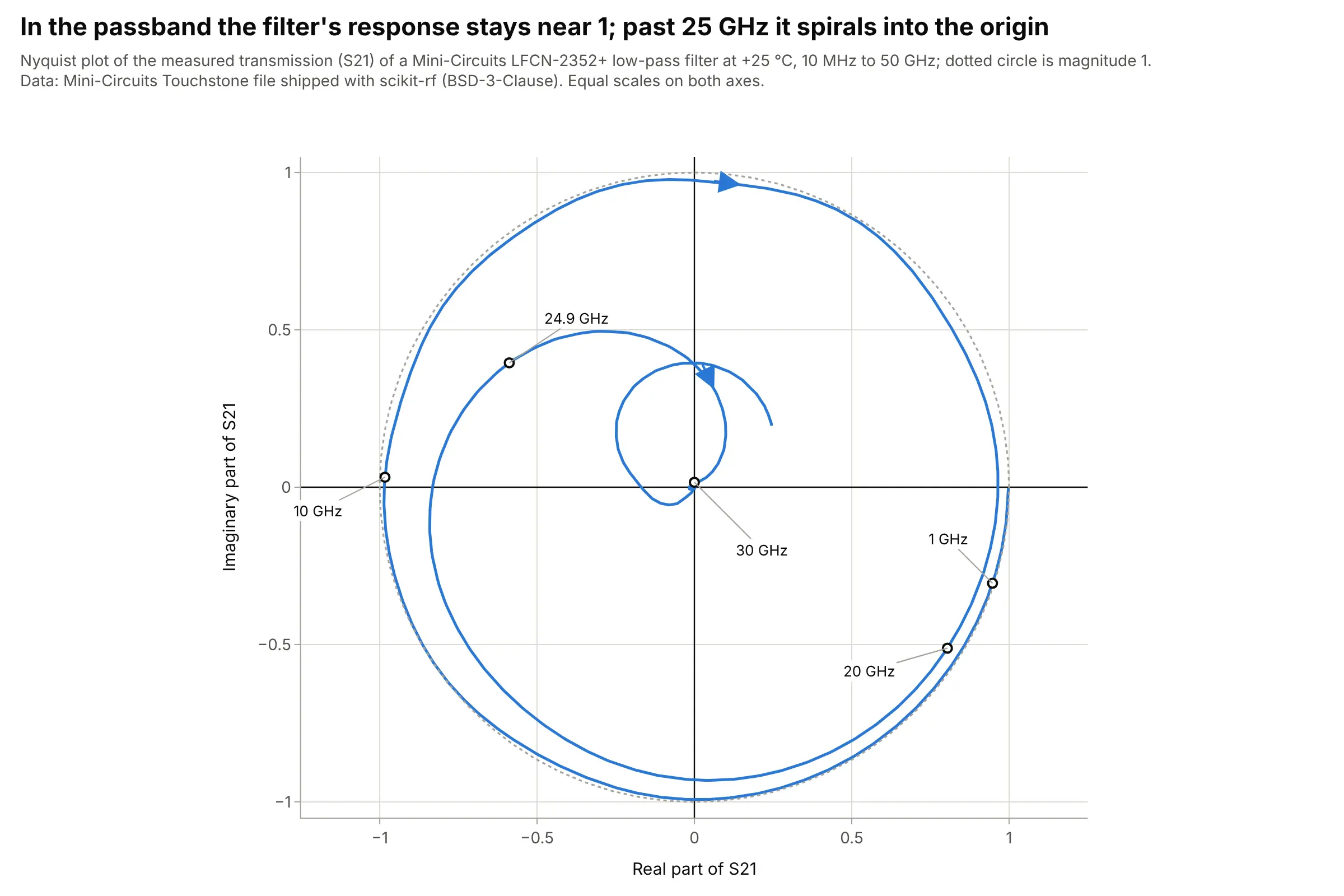
A Mini-Circuits low-pass filter transmits almost all of the signal in its passband (the magnitude of its scattering parameter S21, the transmitted wave, is 0.953 at 20 GHz) and almost none just above it (0.016 at 30 GHz), while its phase keeps turning: 1.59 turns by 24.9 GHz, so the curve winds around the unit circle before it falls into the origin. Data: the Mini-Circuits Touchstone file shipped with scikit-rf (BSD-3-Clause), measured at +25 °C.
Tip: draw the unit circle, so the passband, where the curve hugs it, is easy to tell from the stopband.
Get the data from the Mini-Circuits LFCN-2352+ low-pass filter Touchstone file shipped with scikit-rf(skrf/tests/LFCN-2352+_Plus25degC.s2p: 2,006 frequencies from 10 MHz to 50 GHz, S21 as a complex number).Make a plotly Nyquist plot of S21 with its real part on x and its imaginary part on y, equal scales, a dotted unit circle, andlabels at 1, 10, 20, 24.9 and 30 GHz.
FAQ
Options to customize
A Nyquist plot in Plotly is one go.Scatter trace with an equal-scale axis, so these are the options that matter most. The full lists are in the scatter trace reference, the axes documentation and the annotations documentation.
- fig.update_yaxes(scaleanchor="x", scaleratio=1): equal scales, the rule for a Nyquist plot; add constrain="domain" (the default) to let the plot area shrink to keep the ratio.
- x=z.real, y=z.imag (or y=-z.imag): the two parts of the response; use the negative imaginary part for impedance.
- mode="lines+markers": markers show where each measured frequency falls, which matters for sparse measured data.
- customdata and hovertemplate: put the frequency in the hover text, since it is not on an axis.
- line_dash="dash" with opacity: the mirror image of negative frequencies, drawn fainter than the positive half.
- go.Scatter(x=[-1], y=[0], marker_symbol="x"): the critical point of a control loop.
- fig.add_shape(type="circle", x0=-1, y0=-1, x1=1, y1=1): the unit circle for reading the phase margin; a dotted line is enough.
- fig.add_annotation(..., ax=, ay=): labels with a leader line for frequencies, margins and the arc width.
- xaxis.range and yaxis.range: zoom on the critical point or an arc, and use a second subplot for the whole curve.
- go.Scatter3d with frequency on z: a 3D Nyquist curve when frequency has to stay visible.