
Chris Parmer
November 15, 2026
Lorenz Curves - A Complete Guide
TL;DR
- A Lorenz curve sorts a population from smallest to largest and draws the cumulative share of the people against the cumulative share of the total they hold (income, wealth, gas output, trees, citations), so a straight diagonal means everyone holds the same amount and the more the curve sags below it, the more concentrated the total is.
- Lorenz curves are a cumulative share chart that is similar to Pareto charts, empirical cumulative distribution function (ECDF) plots and the concentration curves of health economics, which rank people by one variable and add up another.
- Read one number off it: the Gini coefficient is twice the area between the curve and the diagonal, from 0 (equal) to 1 (one holder has everything). In the World Bank's latest figures it ranges from 0.24 in the Slovak Republic to 0.54 in South Africa.
- Economists use it for income and wealth, and the same curve shows how concentrated oil and gas wells, tree species, drug spending, bank deposits and scientific citations are, and how flashy a river is.
- You can make a Lorenz curve with Plotly in Python or JavaScript from a sorted cumulative sum and a go.Scatter trace, with a dashed line of equality and square 0% to 100% axes.
What is a Lorenz curve?
Lorenz curves look like this:
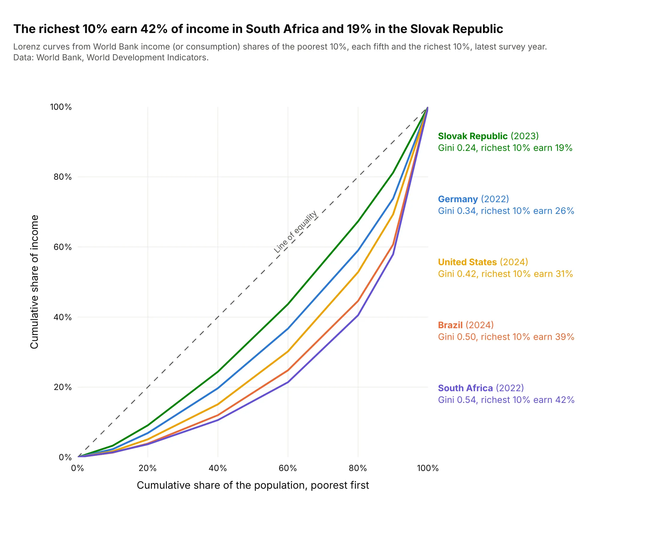
Data: World Bank, World Development Indicators, income (or consumption) shares of the poorest 10%, of each fifth of the population and of the richest 10%, latest survey year of each country.
How do you read a Lorenz curve? In the example above, notice these things:
- A point on a curve says "the poorest x% of people earn y% of the income". In the United States in 2024, the poorest 20% earn 5.1% of income and the richest 20% earn 47.1%, so the point at 80% on the x axis sits at 52.9%.
- The dashed diagonal is the line of equality, where every 10% of the people earn 10% of the income. The Slovak Republic is the closest to it, with the richest 10% earning 18.8%, and South Africa is the farthest, with the richest 10% earning 42.1%.
- The Gini coefficient is twice the area between a curve and the diagonal. The World Bank's Gini is 0.24 for the Slovak Republic and 0.54 for South Africa, computed from household surveys; drawing only these seven published points as straight segments gives slightly lower values (0.23 and 0.52).
- Every curve is flat at the left and steep at the right, because the income of the last tenth of people is the largest single step. The steepest segment is always the last one, from 90% to 100% of the population.
It's often used for charts like these:
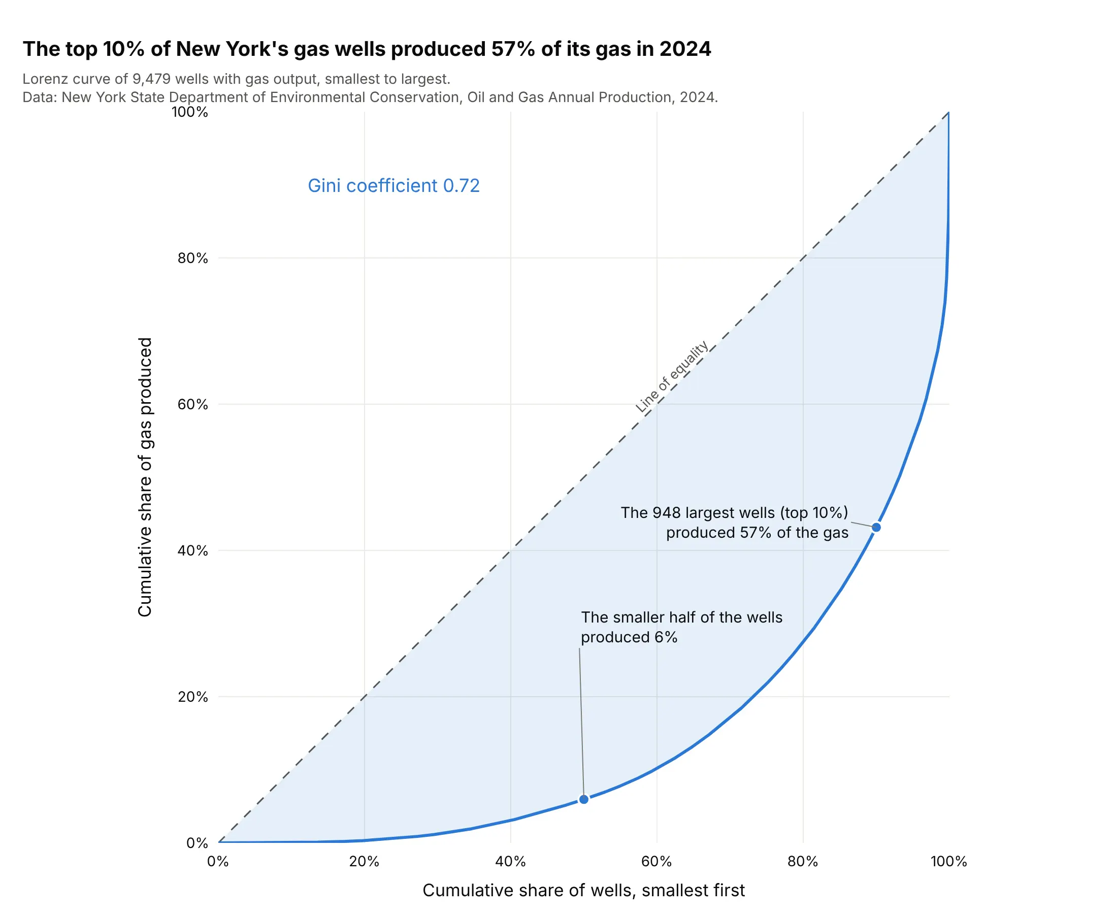
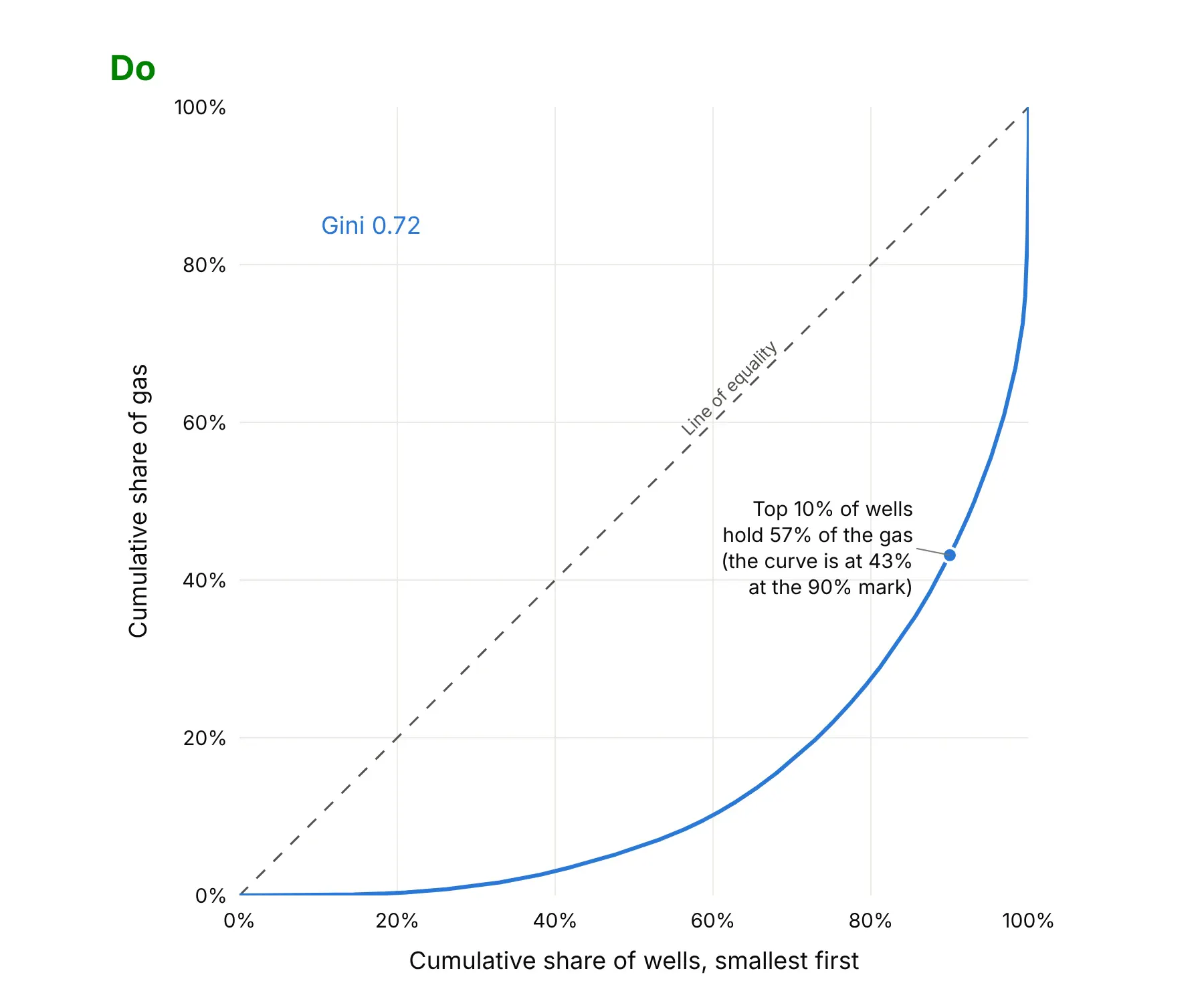
Oil and gas wells. A few wells produce most of a field's output: the top 10% of New York State's 9,479 gas wells produced 57% of its gas in 2024, and the smaller half produced 6%. Data: New York State Department of Environmental Conservation (DEC), Oil and Gas Annual Production, 2024.
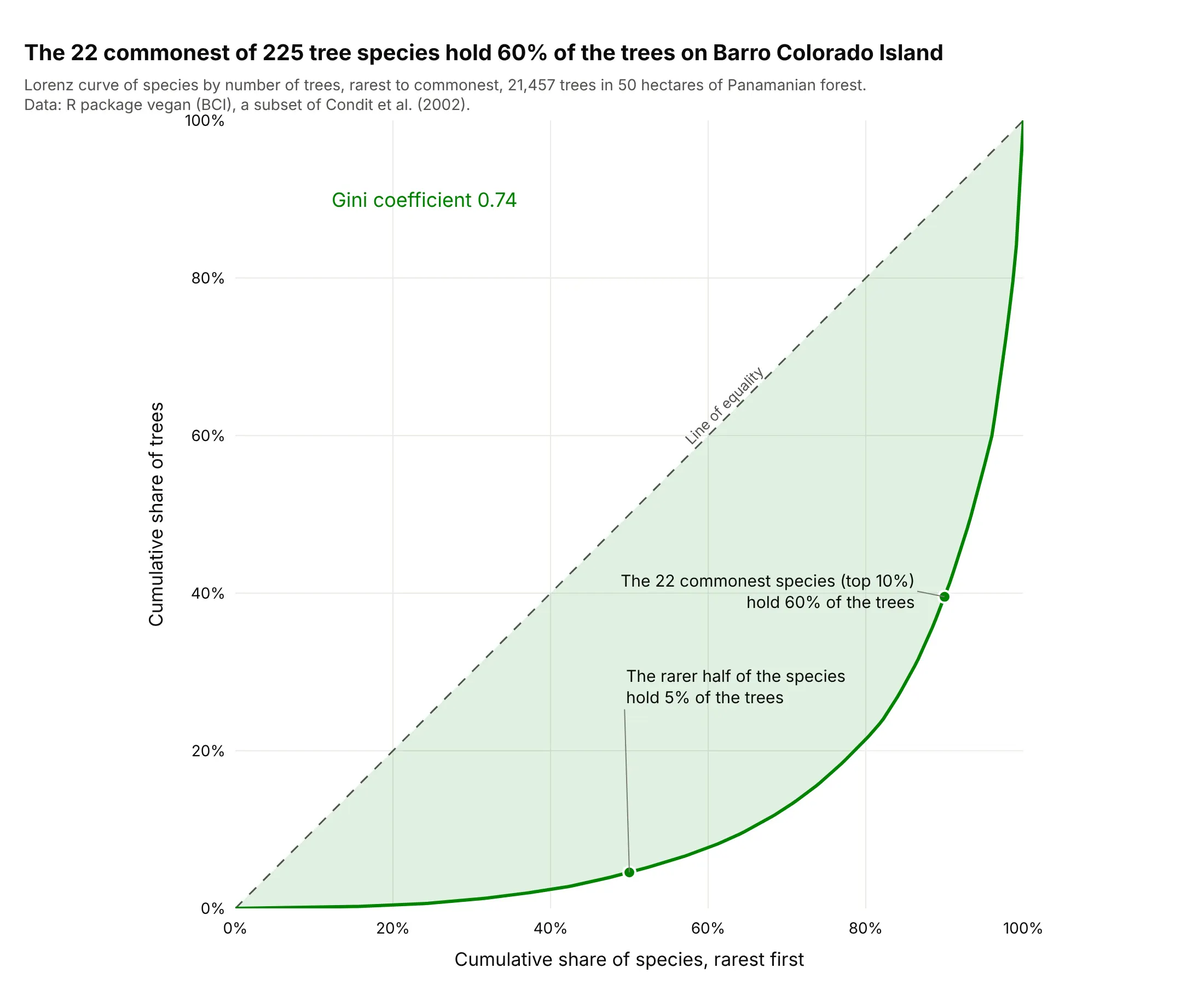
Ecology. Species abundance is the textbook case: the 22 commonest of 225 tree species on Barro Colorado Island in Panama hold 60% of the 21,457 trees, and 19 species have a single tree. Damgaard and Weiner (2000) describe the Lorenz curve for plant size. Data: R package vegan (data set BCI), a subset of Condit et al. (2002).
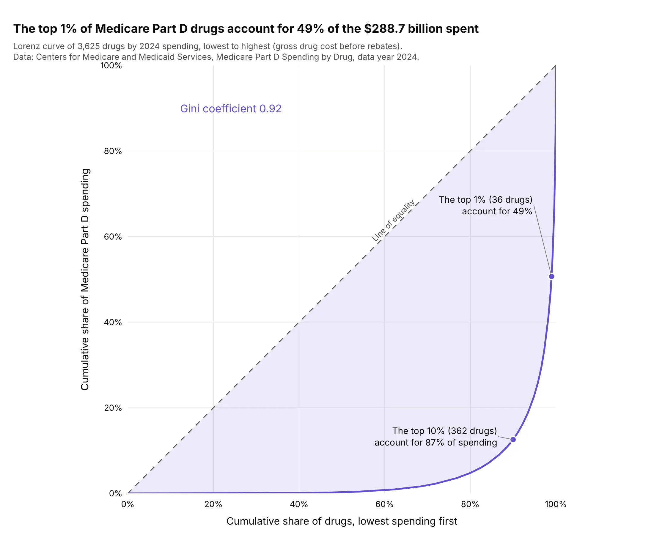
Drug spending. The top 36 of 3,625 drugs account for 49% of the $288.7 billion that Medicare Part D, the US Medicare prescription drug benefit, spent in 2024 (gross cost before rebates), and the top 362 for 87%. Data: Centers for Medicare and Medicaid Services (CMS), Medicare Part D Spending by Drug, data year 2024.
How a Lorenz curve and the Gini coefficient are calculated
A Lorenz curve needs one list of non-negative amounts, one per person (or well, species, article), and four steps. Here they are for five people with illustrative incomes of 10, 15, 20, 25 and 30, which add up to 100:
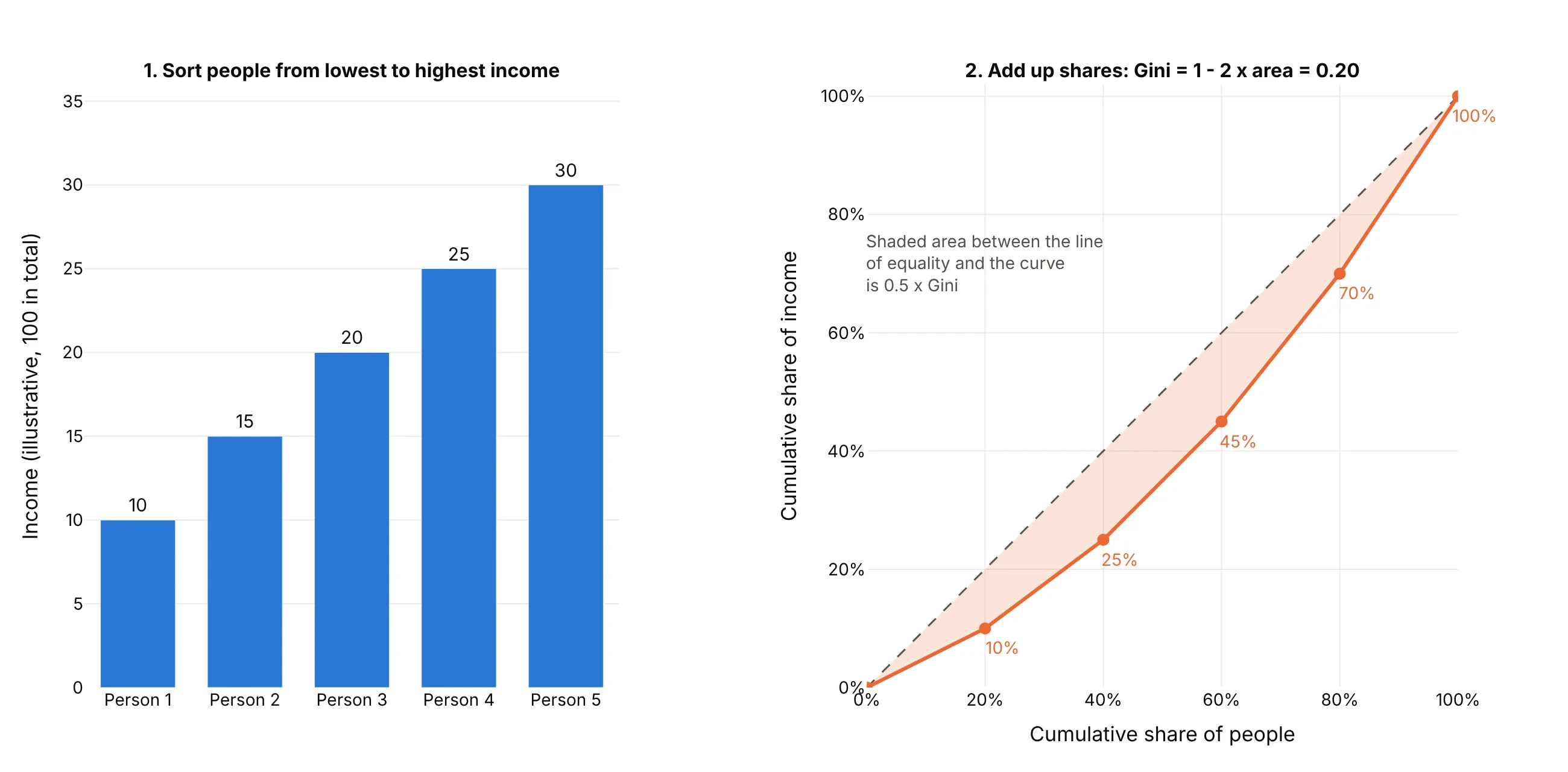
- Sort the people from the lowest amount to the highest.
- Accumulate the amounts and divide by the total. After one person the cumulative share is 10%, after two 25%, then 45%, 70% and 100%.
- Plot the cumulative share of people (20%, 40%, ... 100%) on the x axis against these cumulative shares of the total on the y axis, starting at (0%, 0%), and add the diagonal.
- Measure the area under the curve with trapezoids, and take the Gini coefficient as 1 minus twice that area. Here the area is 0.40 and the Gini coefficient is 0.20. Written as areas, with A the region between the diagonal and the curve and B the region under the curve, the Gini coefficient is A / (A + B), and since A + B is always 0.5, that is 2A, or 1 - 2B.
A Gini coefficient of 0 means every person holds the same amount, and a value near 1 means one holder has nearly everything. For a finite list, the highest possible value is 1 - 1/n, so it can't reach exactly 1 (with five people, the maximum is 0.8). The curve is a smooth function only for very large populations; with a list of values it is a set of straight segments.
What different Gini coefficients look like
It helps to see the curve at known values. This figure draws synthetic lognormal incomes, a distribution whose Lorenz curve has an exact formula, at four Gini coefficients, with the share held by the top tenth beside each:
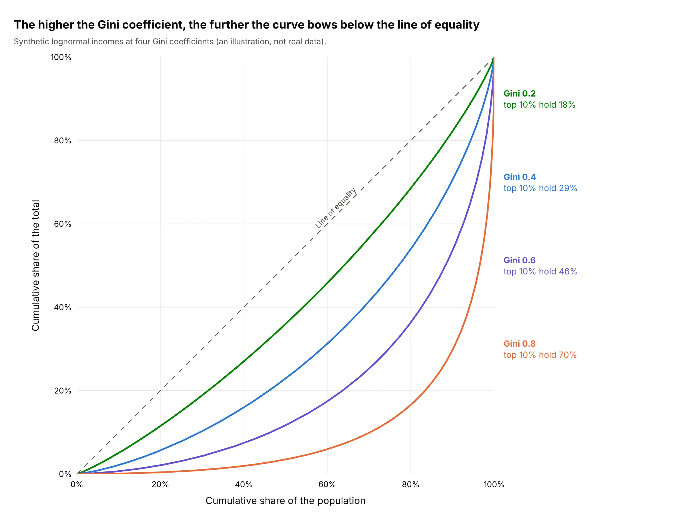
- 0.2: the curve hugs the diagonal, and the top tenth holds 18%. The Slovak Republic is near here (0.24).
- 0.4: the curve sags visibly, and the top tenth holds 29%. The United States (0.42) is here.
- 0.6 to 0.8: the top tenth holds 46% to 70%, and most of the total sits in the last few percent of the population. Brazil (0.50) and South Africa (0.54) are just below this range, and New York's gas wells (0.72) and tree species (0.74) are in it.
- 0.9 and above: the curve runs along the bottom and then shoots up at the right edge, as for Medicare Part D drugs (0.92) and US bank deposits (0.93).
When two curves cross
The Gini coefficient squeezes a whole curve into one number, so two different curves can share a value. The curves in example 4 below show it: the Guadalupe and Potomac rivers cross near the highest tenth of days, because the Guadalupe has a lower Gini coefficient (0.41 against 0.51) but a heavier burst on its very highest days. When one curve lies entirely above another and they never cross, and the two groups have the same mean, Atkinson (1970) showed that the ranking is the same for every standard inequality measure of the usual kind. When they cross, the ranking depends on which part of the distribution you care about, so show the curves and not only the Gini coefficients.
A short history
Max Lorenz proposed the curve in 1905 to show how concentrated wealth is, in "Methods of Measuring the Concentration of Wealth" in the Publications of the American Statistical Association. The Italian statistician Corrado Gini published the coefficient in his 1912 paper Variabilità e mutabilità, building on Lorenz's diagram, according to Wikipedia's Gini coefficient article. Economists then used the pair for income and wealth, and ecologists, biodiversity researchers, epidemiologists and credit-risk analysts adopted the same construction for their own totals, as Wikipedia's Lorenz curve article lists. We couldn't find the data behind Lorenz's original examples in a public form to redraw them, so the main example above uses current World Bank figures instead.
Alternatives to a Lorenz curve
Here's the same set of 9,479 gas wells drawn six ways. Some are better for the question, some worse, some just different:
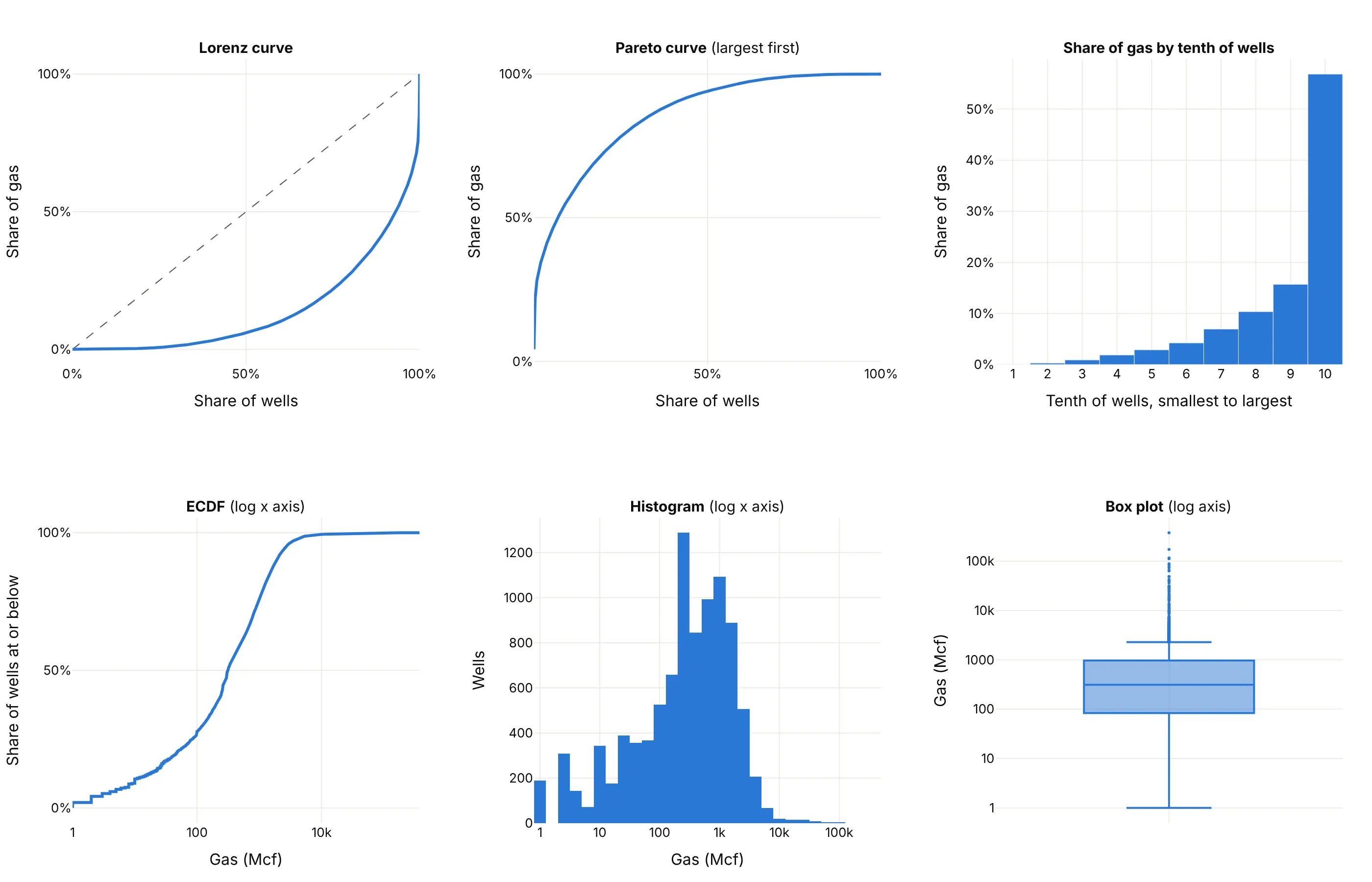
- Pareto chart (works too, and it is the same curve upside down). It sorts from the largest and accumulates, so the Pareto curve at a rank share k equals 1 minus the Lorenz curve at 1 - k. It is the better choice when the reader wants to know which items make up most of the total, because the items are named along the x axis. The Lorenz curve is better for comparing several groups on one 0% to 100% square and for reading the Gini coefficient.
- ECDF plot (different). An ECDF plots the share of wells at or below each output, with output on the x axis. A Lorenz curve plots the share of wells against the share of the gas those wells produce, so it weights every well by its size. The ECDF shows the typical well, and the Lorenz curve shows who holds the total.
- Bar chart of shares by tenth (works too, for a general audience). The top tenth produces 57% and the bottom five tenths under 6%, which is easy to say aloud, but the bars lose the shape inside each tenth and can't give a Gini coefficient.
- Histogram (different). On a log axis it shows the typical output of 300 to 1,000 thousand cubic feet (Mcf), but not how much of the gas the long tail adds up to.
- Box plot (worse). It marks the large wells as outliers, which are in fact where most of the gas is.
How to make a Lorenz curve
With AI
ChatGPT, Claude Code, GitHub Copilot, Cursor and other AI tools are excellent at writing Plotly code. Name Plotly in the prompt, and say how to sort, what the axes are and what to annotate:
Make a plotly Lorenz curve from wells.csv (columns: api_wellno, gas_mcf, the 2024 gas production of each well).- Keep wells with gas_mcf above 0, sort them from smallest to largest, and plot the cumulative share of wells(x, starting at 0) against the cumulative share of gas (y) as a go.Scatter line with a light fill to the diagonal.- Add a dashed line of equality, set both axes to 0% to 100% with tickformat ".0%", and make the plot square withyaxis scaleanchor "x" and xaxis constrain "domain".- Compute the Gini coefficient as 1 - 2 x the trapezoid area under the curve and write it on the chart.- Label the point where the largest 10% of wells are, with the share of gas they produced.- Axis titles: "Cumulative share of wells, smallest first" and "Cumulative share of gas". A title that states the takeaway.- Check: print the share of gas from the top 10% of wells and the Gini coefficient.
With Plotly Studio
Plotly Studio is a product for creating data visualizations and Dash apps and for analyzing data with AI, available as a desktop app or embedded in Dash apps. Ask for a Lorenz curve the same way:
Show a Lorenz curve of income by country from the World Bank income shares, with a dropdown to pick countries, a dashed line of equality, a square 0% to 100% plot, and each country's Gini coefficient and the share earned by the richest 10% in the legend.
Make a Lorenz curve in Python or JavaScript
This is the code AI tools write under the hood. In Python, sorting and a cumulative sum give the curve, and a go.Scatter trace with fill="tonexty" shades the area between it and the diagonal. This uses the tree counts of the Barro Colorado Island example (one row per species):
import numpy as npimport pandas as pdimport plotly.graph_objects as gotrees = pd.read_csv("bci_trees.csv")["trees"] # one row per species: number of treesv = np.sort(trees.to_numpy()) # smallest firstx = np.arange(len(v) + 1) / len(v) # cumulative share of speciesy = np.concatenate([[0], np.cumsum(v)]) / v.sum() # cumulative share of treesgini = 1 - 2 * np.trapezoid(y, x) # np.trapz in NumPy 1.xfig = go.Figure([go.Scatter(x=[0, 1], y=[0, 1], mode="lines", line=dict(dash="dash", color="gray"), name="Line of equality"),go.Scatter(x=x, y=y, mode="lines", fill="tonexty", name="Species"),])fig.update_layout(title=f"Gini coefficient {gini:.2f}", showlegend=False, width=700, height=700,xaxis=dict(title="Cumulative share of species, rarest first", tickformat=".0%", range=[0, 1], constrain="domain"),yaxis=dict(title="Cumulative share of trees", tickformat=".0%", range=[0, 1], scaleanchor="x"),)fig.show()
The scaleanchor and constrain settings make the plot square, so the diagonal is a true 45° line and the area between the curve and the diagonal reads the same whatever the window size. The Gini coefficient from this code is 0.74, the value shown in the Barro Colorado Island example. If your data are already group shares, such as the World Bank's fifths of the population, build x from the group boundaries and y from the cumulative sums of the shares, as the JavaScript below does.
In JavaScript, plotly.js draws the same chart from arrays. This version uses the World Bank's income shares for Brazil in 2024 (the poorest 10%, each fifth of the population and the richest 10%):
<div id="chart"></div><script src="https://cdn.plot.ly/plotly-4.1.1.min.js"></script><script>// Brazil 2024, World Bank income shares (%): lowest 10%, five fifths, highest 10%const lowest10 = 1.3, fifths = [3.9, 8.1, 12.8, 19.8, 55.4], highest10 = 39.3;// Cumulative population at the published points (10%, 20%, 40%, 60%, 80%, 90%, 100%) and the income held by themconst x = [0, 0.1, 0.2, 0.4, 0.6, 0.8, 0.9, 1];const cum = [0, lowest10];let run = 0;fifths.forEach(s => { run += s; cum.push(run); });const y = [cum[0], cum[1], cum[2], cum[3], cum[4], cum[5], 100 - highest10, 100].map(v => v / 100);// Gini = 1 - 2 x area under the curve (trapezoids). This is lower than the survey Gini of 0.50 because// the curve between the published points is drawn straight.let area = 0;for (let i = 1; i < x.length; i++) area += (x[i] - x[i - 1]) * (y[i] + y[i - 1]) / 2;Plotly.newPlot("chart", [{x: [0, 1], y: [0, 1], mode: "lines", line: {dash: "dash", color: "gray"}, name: "Line of equality"},{x: x, y: y, mode: "lines+markers", line: {width: 3}, name: "Brazil, 2024"}], {width: 700, height: 700, showlegend: false,title: {text: "Brazil, 2024: Gini from these points = " + (1 - 2 * area).toFixed(2)},xaxis: {title: {text: "Cumulative share of the population"}, tickformat: ".0%", range: [0, 1], constrain: "domain"},yaxis: {title: {text: "Cumulative share of income"}, tickformat: ".0%", range: [0, 1], scaleanchor: "x"}});</script>
For several groups, add one trace per group, as the five-country and five-river examples do, and label each line at its right end instead of using a legend.
Share it
Every Plotly chart has a Share chart button (the cloud icon in its toolbar) that uploads it to Plotly Cloud and gives you a link. Only you can see it until you change its visibility.
For a live app, put the chart in a Dash app and publish it with the Plotly Cloud command-line interface (CLI). Coding agents can run these commands for you:
pip install "dash[cloud]"plotly user loginplotly app publish
If your data has to stay in your own cloud or data center, publish to Dash Enterprise instead.
Dos and don'ts
A Lorenz curve is only readable against its diagonal, and it only means something when the axes are on the same 0% to 100% scale. Here are the New York gas wells both ways, in the same blue.
Don't leave out the line of equality, stretch the plot so it is wider than tall (which changes how far the curve looks from the diagonal), leave the axes as raw 0 to 1 numbers with an axis that runs to 1.2, label them only x and y, use a serif font, or join thousands of points with large markers, which merge into a thick band:
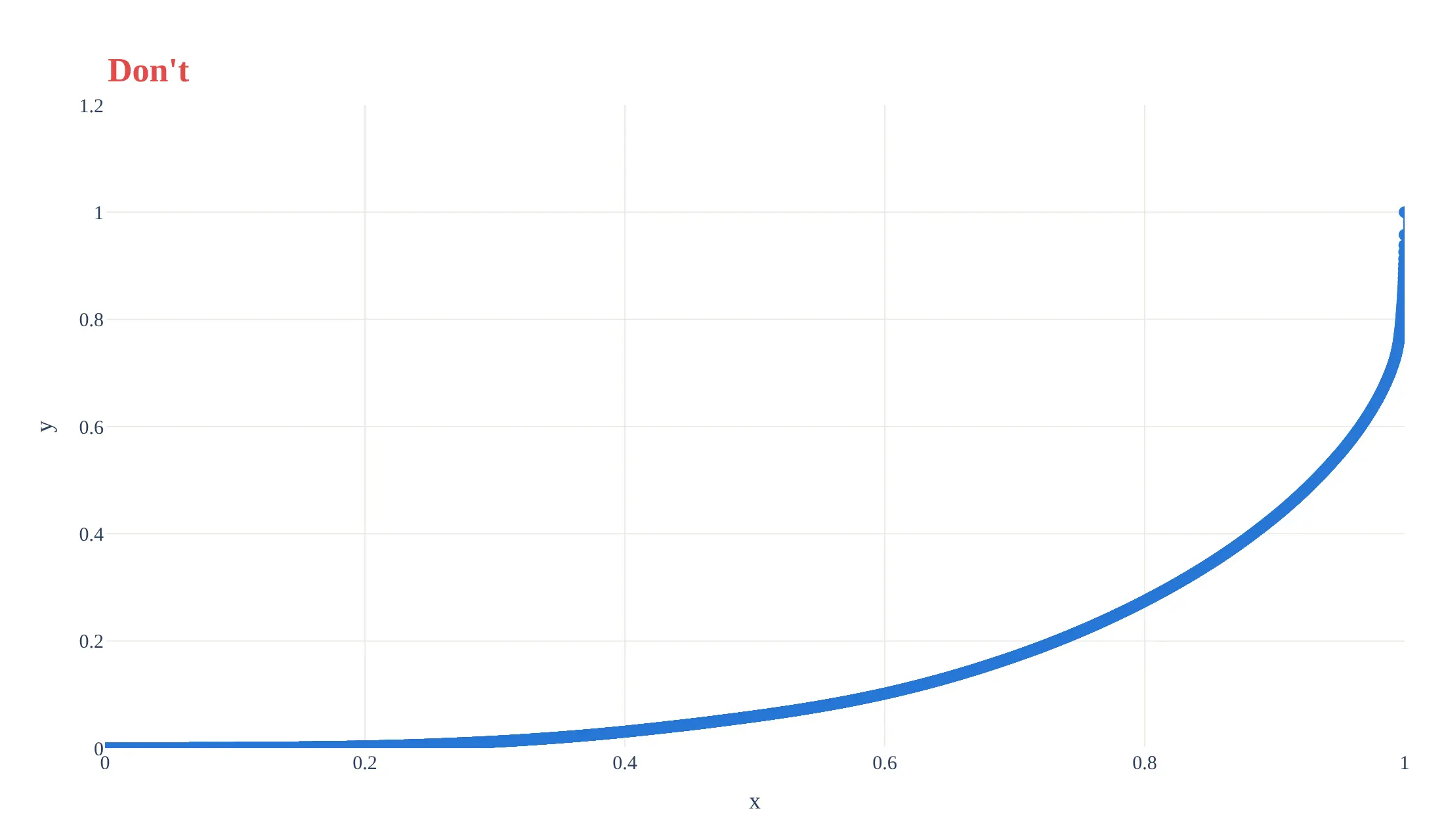
Do draw a thin line without markers, add the dashed line of equality, make the plot square with both axes from 0% to 100%, write the axis titles in words (what is accumulated and in which order), and label one point with the number a reader can quote:
Checklist
Do
- Say which way you sorted ("smallest first") and what the x and y axes accumulate.
- Draw the line of equality, and use equal 0% to 100% axes so the plot is square.
- Print the Gini coefficient and one or two readable points, such as the share held by the top 10%.
- Use the same colors for the same group across charts, and label curves at their ends when you compare several.
- State what the units are (people, households, wells, species) and whether the data are income, consumption or wealth.
- Say how the curve was built when the data are grouped (here, straight segments between seven published points).
Don't
- Sort the wrong way round. A curve above the diagonal usually means the data were sorted from largest to smallest.
- Compare Gini coefficients from different sources or definitions (income against consumption, before or after taxes) without saying so.
- Read a lone Gini coefficient as a full description, since different curves share the same value.
- Use markers on a curve with thousands of points.
More Lorenz curve examples
Six more Lorenz curves built from real public data, each with its source, the technique that makes it work and a prompt to rebuild it.
1. Brazil's curve moved toward the line of equality
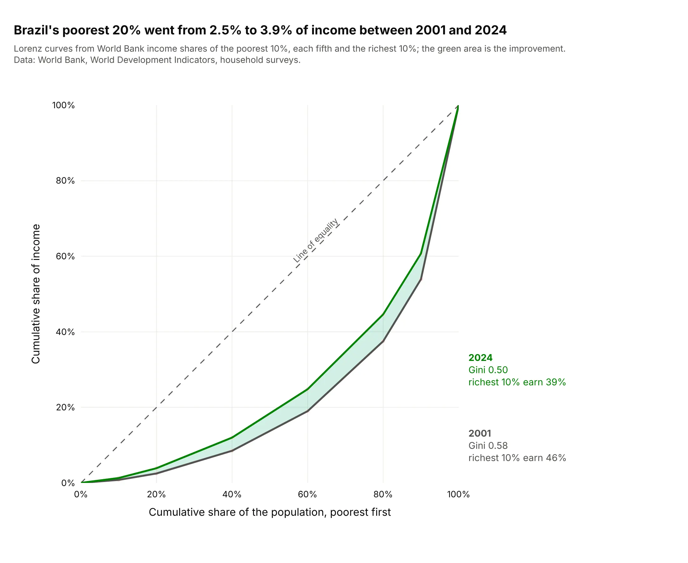
Between 2001 and 2024, the poorest 20% of Brazilians went from earning 2.5% to 3.9% of income and the richest 10% from 46.1% to 39.3%. The World Bank's Gini coefficient fell from 0.58 to 0.50, and the shaded area is the change. Data: World Bank, World Development Indicators (SI.DST and SI.POV.GINI series), household surveys.
Tip: shade the area between two years' curves, because the gap is the change and the reader doesn't have to compare two Gini coefficients.
Get the data from the World Bank World Development Indicators bulk downloads (indicators SI.DST.FRST.10, SI.DST.FRST.20,SI.DST.02ND.20, SI.DST.03RD.20, SI.DST.04TH.20, SI.DST.05TH.20, SI.DST.10TH.10 and SI.POV.GINI) for Brazil(columns: year, d1, q1, q2, q3, q4, q5, d10, gini).Build a plotly Lorenz curve of 2001 against 2024 on a square 0% to 100% plot: x = 0, 10%, 20%, 40%, 60%, 80%, 90%, 100%,y = the cumulative income shares, with the lowest-10% share and 100 minus the highest-10% share at 10% and 90%. Shade the area betweenthe two curves and label each line with its year, Gini coefficient and the richest 10%'s share.
2. The largest 10% of US banks hold 91% of domestic deposits
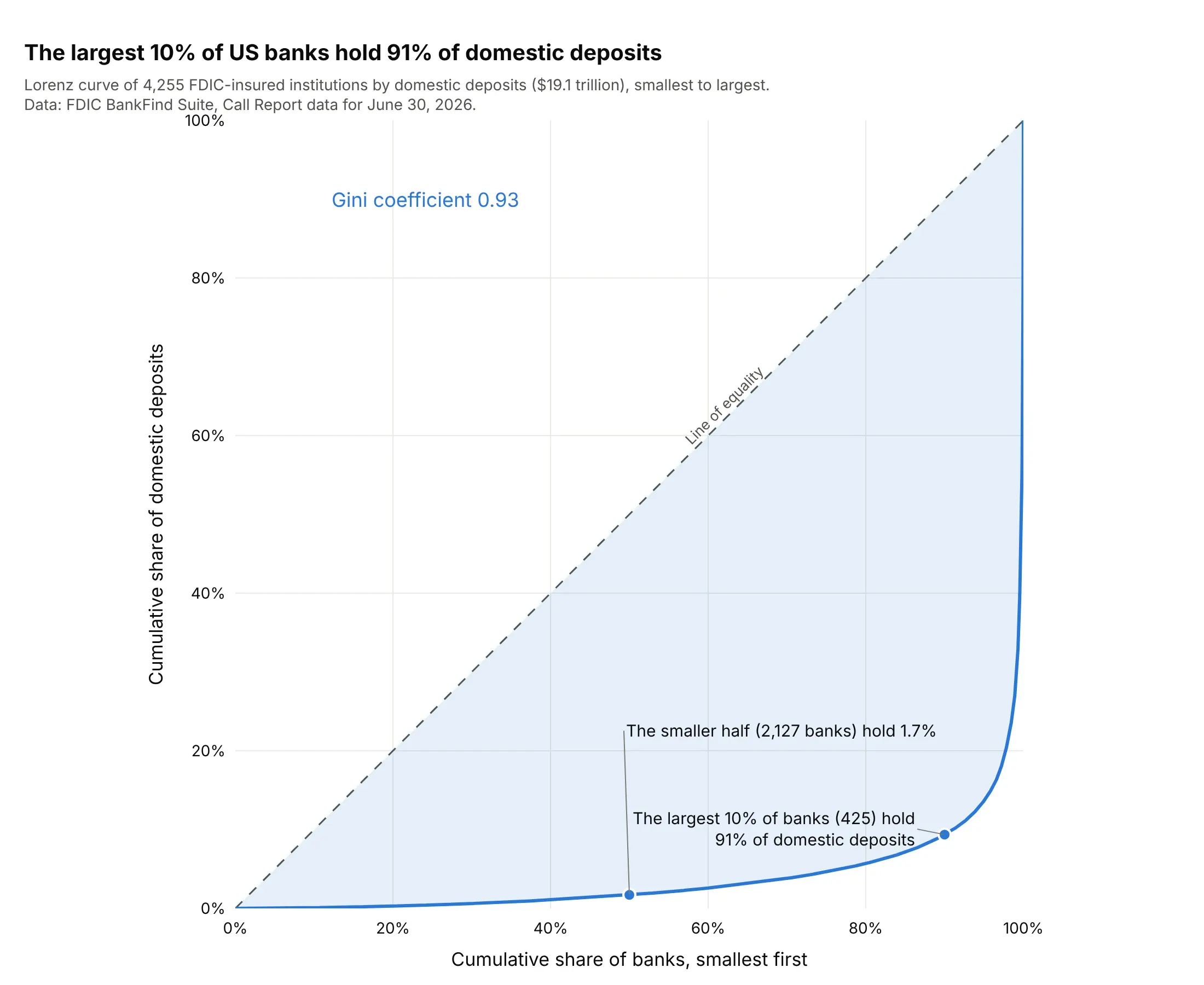
Market concentration is usually quoted as the share of the top few firms, and the curve shows the whole market: 425 of 4,255 institutions hold 91% of $19.1 trillion in domestic deposits, while the smaller half holds 1.7%. The Gini coefficient is 0.93. Data: Federal Deposit Insurance Corporation (FDIC), BankFind Suite Call Report data, domestic deposits (DEPDOM), June 30, 2026.
Tip: when the curve runs along the bottom edge, label the smaller half's share ("1.7%"), because the eye can't read it off the axis.
Get the data from the FDIC BankFind Suite API (https://api.fdic.gov/banks/financials), all institutions with report date2026-06-30 and field DEPDOM (domestic deposits in thousands of dollars) (columns: cert, name, state, domestic_deposits_k).Build a plotly Lorenz curve of banks with positive deposits sorted from smallest to largest, on a square 0% to 100% plot,with the Gini coefficient written on it, one label for the largest 10% of banks and their share, and one for the smaller half.
3. Citations of scientific articles
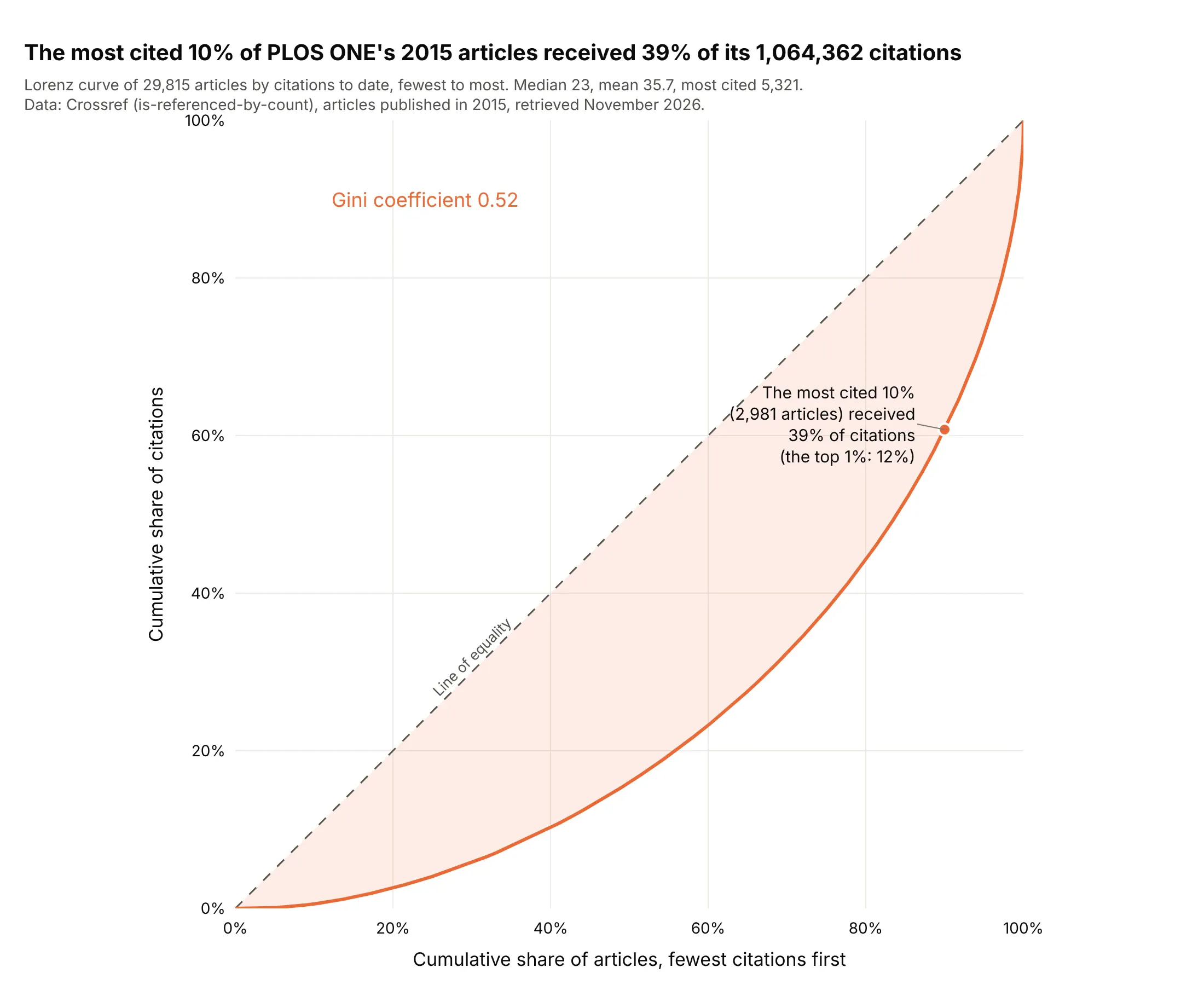
Citation counts are the classic skewed quantity in science, described in Seglen's "The skewness of science" (1992). Of 29,815 articles published in PLOS ONE (Public Library of Science) in 2015, the most cited 10% received 39% of the 1,064,362 citations to date, and the mean (35.7) is above the median (23). The Gini coefficient is 0.52, much lower than for wells or banks. Data: Crossref REST API (is-referenced-by-count), PLOS ONE articles published in 2015, retrieved November 2026.
Tip: put the mean and median in the subtitle, because their gap is the same story as the curve in two numbers.
Get the data from the Crossref REST API (https://api.crossref.org/works): every journal article of PLOS ONE (ISSN 1932-6203)published from 2015-01-01 to 2015-12-31, fields DOI and is-referenced-by-count, using cursor paging with 1,000 rowsa page (columns: doi, citations).Build a plotly Lorenz curve of articles sorted from fewest to most citations, on a square 0% to 100% plot, with a lightfill to the diagonal, the Gini coefficient, one label for the most cited 10% and their share of citations, and the median and mean in the subtitle.
4. How evenly a river's water arrives over a year
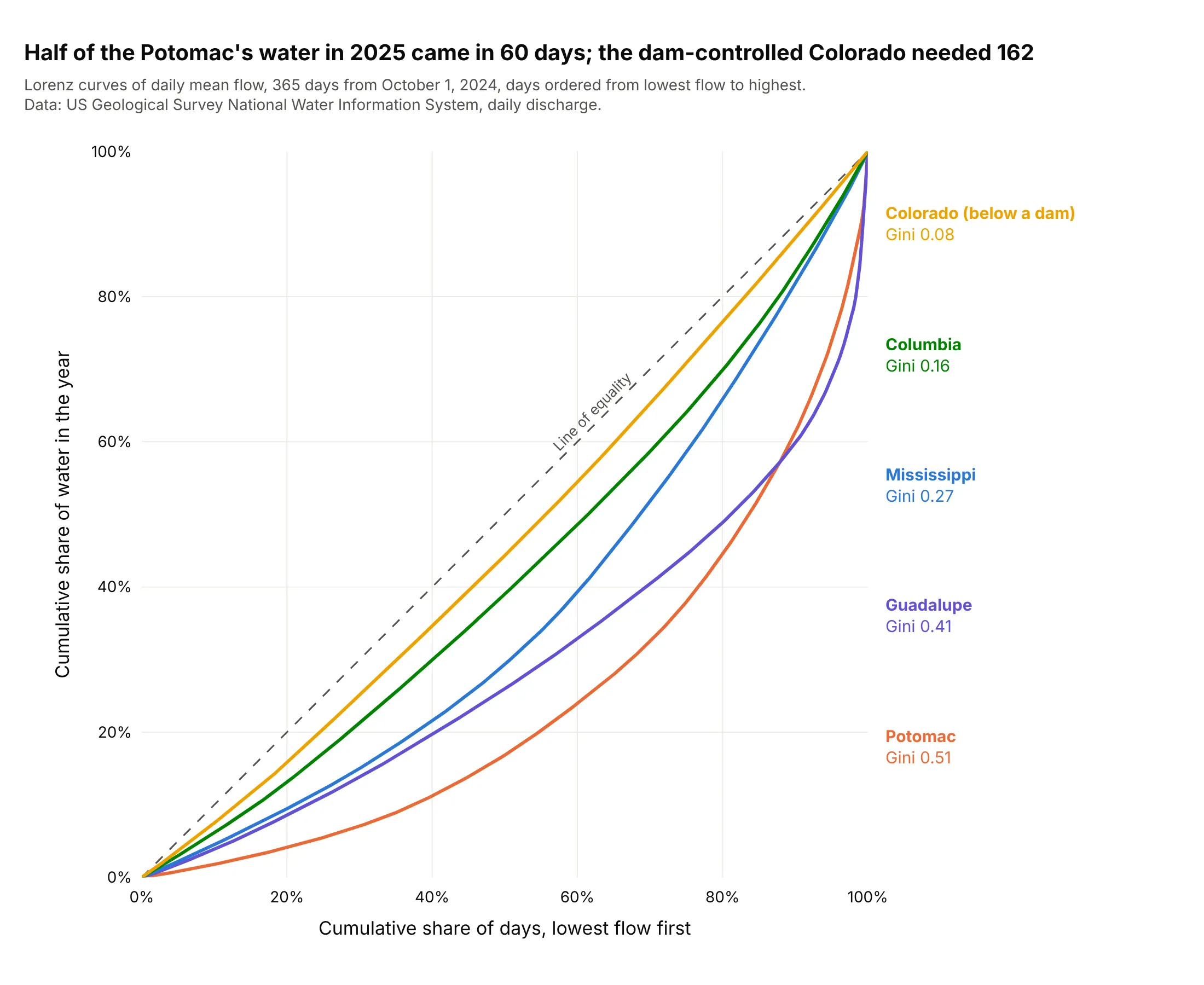
Here the population is the 365 days and the total is the year's water. The Colorado below Glen Canyon Dam is almost on the diagonal (Gini 0.08, half its water in 162 days), while the Potomac received half of its water in 60 days (Gini 0.51), and the Guadalupe and Potomac curves cross near the highest tenth of days. Data: US Geological Survey (USGS), National Water Information System daily mean discharge, October 1, 2024 to September 30, 2025.
Tip: label each curve with its Gini coefficient at the right of the plot, in the order of the lines, so the reader doesn't need a legend.
Get the data from the USGS National Water Information System daily values service (https://waterservices.usgs.gov/nwis/dv/),parameter 00060 (discharge in cubic feet per second), statistic 00003 (daily mean), for sites 09380000, 14105700, 07010000,08176500 and 01646500, from 2024-10-01 to 2025-09-30 (columns: date, river, cfs).Build a plotly chart with one Lorenz curve per river (days sorted from lowest to highest flow, on a square 0% to 100% plot),a dashed line of equality, and labels at the right with each river's name and Gini coefficient.
5. Solar plants are more concentrated than wind plants
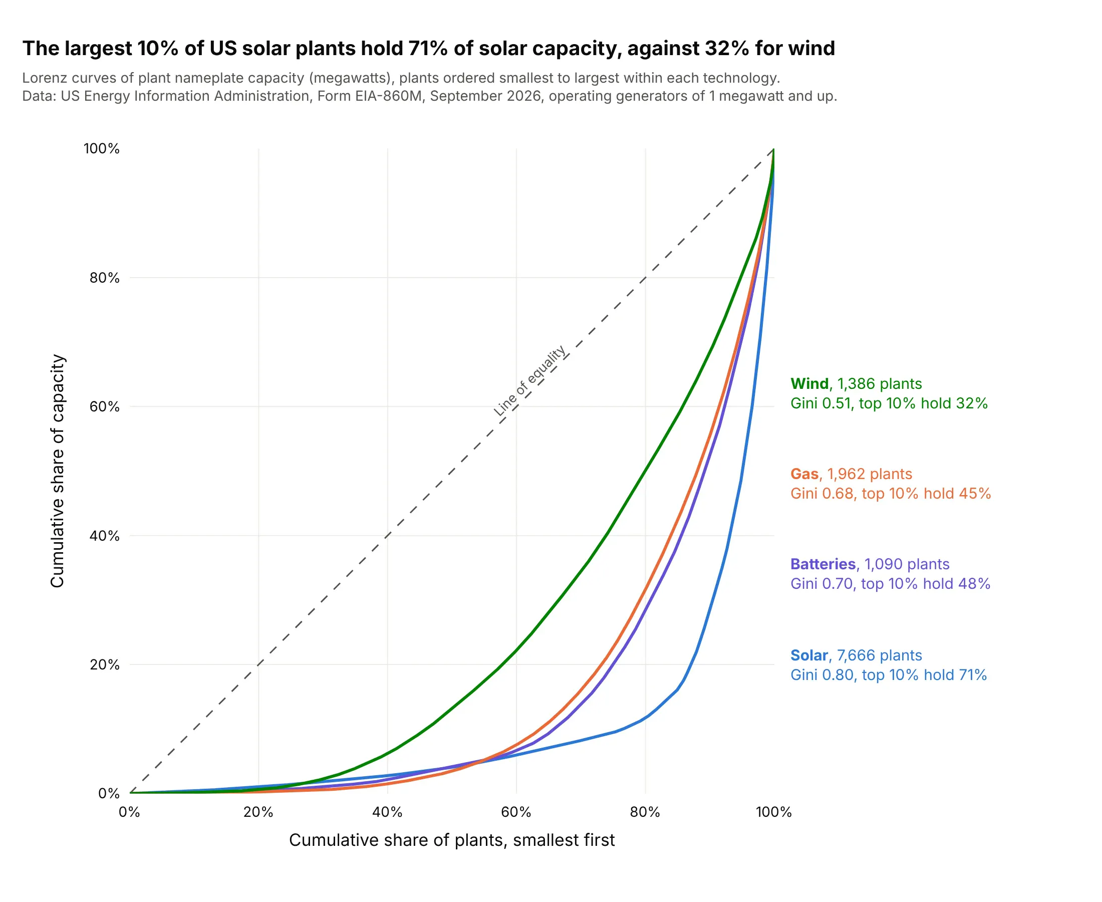
Solar has 7,666 operating US plants, and the largest 10% hold 71% of the 170.6 gigawatts (GW), while the 1,386 wind plants are far more even (Gini 0.51, top 10% hold 32%). Gas and batteries sit between them. Data: US Energy Information Administration (EIA), Form EIA-860M (monthly generator inventory), September 2026, operating generators of 1 megawatt (MW) and up.
Tip: to compare groups with very different counts, put them on one square plot and give each its own count in the label.
Get the data from the US EIA Form EIA-860M, September 2026, sheet "Operating" (https://www.eia.gov/electricity/data/eia860m/):group generators by plant and technology (Solar Photovoltaic, Onshore and Offshore Wind Turbine, Batteries, every"Natural Gas" technology except compressed air) and sum the nameplate capacity in megawatts (columns: plant_id, plant, state, tech, mw).Build a plotly chart with one Lorenz curve of plant capacity per technology on a square 0% to 100% plot, each labeled at theright with its plant count, Gini coefficient and the share held by the largest 10% of plants.
6. Signal processing: a photo's energy sits in few transform coefficients
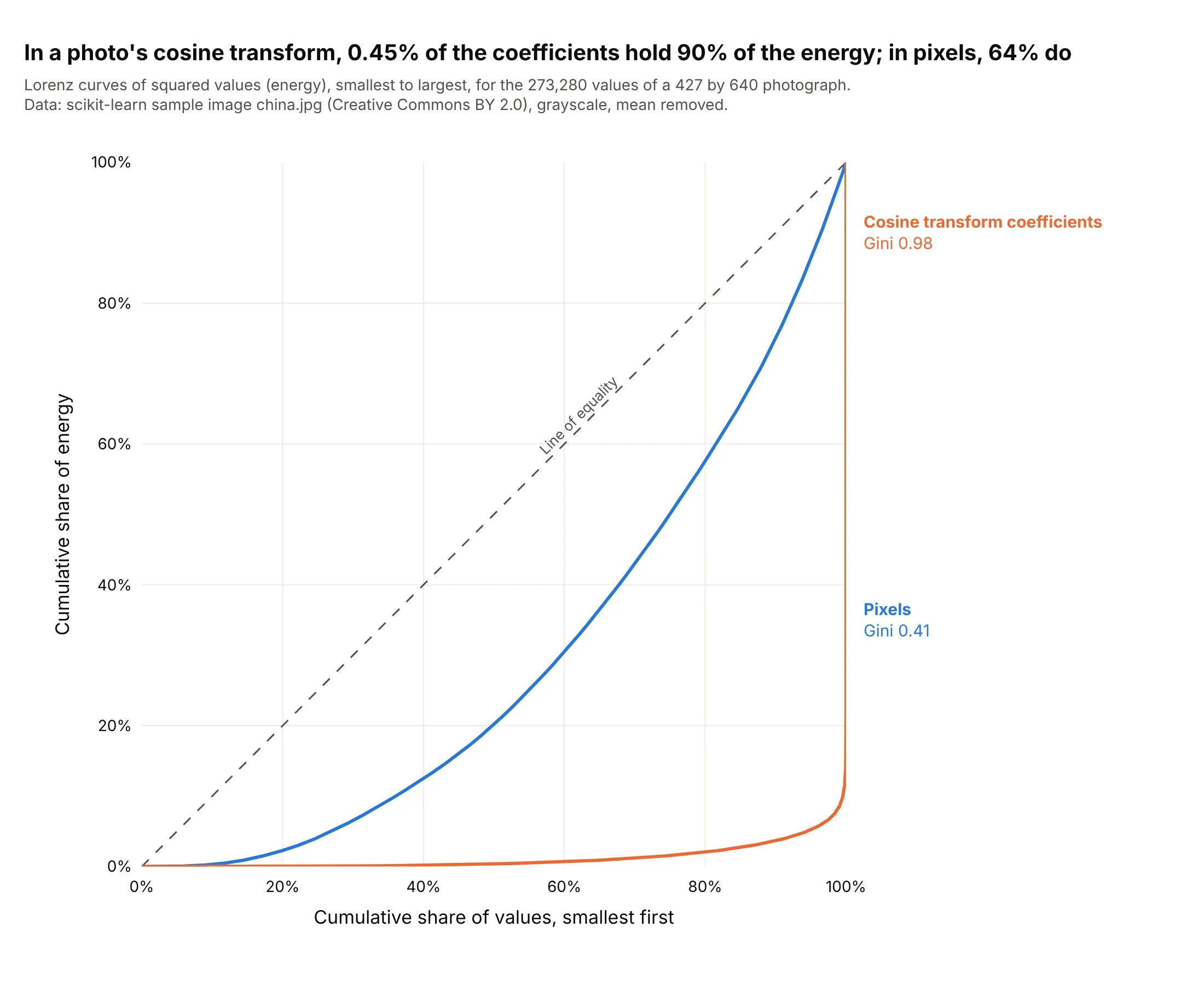
In engineering, the Gini index is a measure of sparsity (Hurley and Rickard, 2009). Taking a sample photograph of 273,280 pixels, 64% of the pixels are needed to hold 90% of the energy (squared values, mean removed), but after the discrete cosine transform that JPEG (Joint Photographic Experts Group) compression is built on, 1,237 coefficients (0.45%) hold it. Data: scikit-learn's sample image china.jpg (Creative Commons BY 2.0, by danielbuechele on Flickr), grayscale.
Tip: put both domains on one plot with the same sort order, because the gap between the two curves is the compression gain.
Use scikit-learn's sample photograph (sklearn.datasets.load_sample_image("china.jpg")), convert it to gray with weights0.299, 0.587 and 0.114, subtract the mean, and compute its 2D discrete cosine transform with scipy.fft.dctn(norm="ortho").Build a plotly chart with two Lorenz curves of the squared values (energy), one for the pixels and one for the cosinecoefficients, each sorted smallest first on a square 0% to 100% plot, with the Gini coefficient of each on the chart and the number of coefficients that hold 90% of the energy.
FAQ
Options to customize
A Lorenz curve in Plotly is a line trace of cumulative shares plus a diagonal, so these are the options that matter most. The full lists are in the scatter trace reference and the layout reference.
- np.cumsum(np.sort(values)) / values.sum(): the curve itself, with a 0 in front so it starts at the origin; np.trapezoid(y, x) gives the area for the Gini coefficient.
- go.Scatter(mode="lines"): the curve, with line.width of 3 and no markers when there are more than a few dozen points.
- fill="tonexty" (or fill="toself" with a closed path): shades the Gini area between the curve and the diagonal, or the gap between two years' curves.
- A diagonal trace from (0, 0) to (1, 1) with line.dash="dash": the line of equality.
- xaxis.tickformat=".0%", yaxis.tickformat=".0%", range=[0, 1]: percent axes from 0% to 100%.
- yaxis.scaleanchor="x", xaxis.constrain="domain": equal scales, so the plot is square and the diagonal is a 45° line.
- add_annotation with ax, ay: labels with leader lines on the points a reader will quote (the top 10%, the smaller half).
- hovertemplate: "%{x:.0%} of wells produce %{y:.1%} of the gas", so hovering reads as a sentence.
- customdata: the name of the unit (species, drug, bank) at each point, for the hover text.
- xaxis.domain: leaves room at the right for direct labels when you compare several groups.
- make_subplots with shared_yaxes=True: one Lorenz curve per year or region side by side when overlapping lines would be too many.