
Chris Parmer
November 18, 2026
Flame Graphs - A Complete Guide
TL;DR
- A flame graph is a picture of where a program spends its time, drawn from thousands of stack samples, which are snapshots of the chain of function calls that was running at one instant: each box is a function, its width is the share of samples that include it, its height is how deep it sits in the call stack, and the left to right order is alphabetical, not time.
- Flame graphs are also written flamegraphs, and drawn upside down they are icicle graphs. When time is on the x axis the chart is a flame chart, which is a different chart. They are similar to icicle charts, sunburst charts and treemaps.
- Read them for wide boxes and for flat plateaus at the top of a tower, because the top edge is the code that was actually running. In the pandas profile below, a function we wrote takes 22% of the samples and a pandas internal called _sorted_data takes 44%. The colors are random warm hues and mean nothing.
- Software engineers use them to find the function worth optimizing, and differential flame graphs (red where a change added samples, blue where it removed them) to check what a change did.
- You can make one with Plotly in Python or JavaScript from a go.Icicle trace with tiling=dict(orientation="v", flip="y"), fed by a profile recorded with a tool such as py-spy.
What is a flame graph?
This is a flame graph:
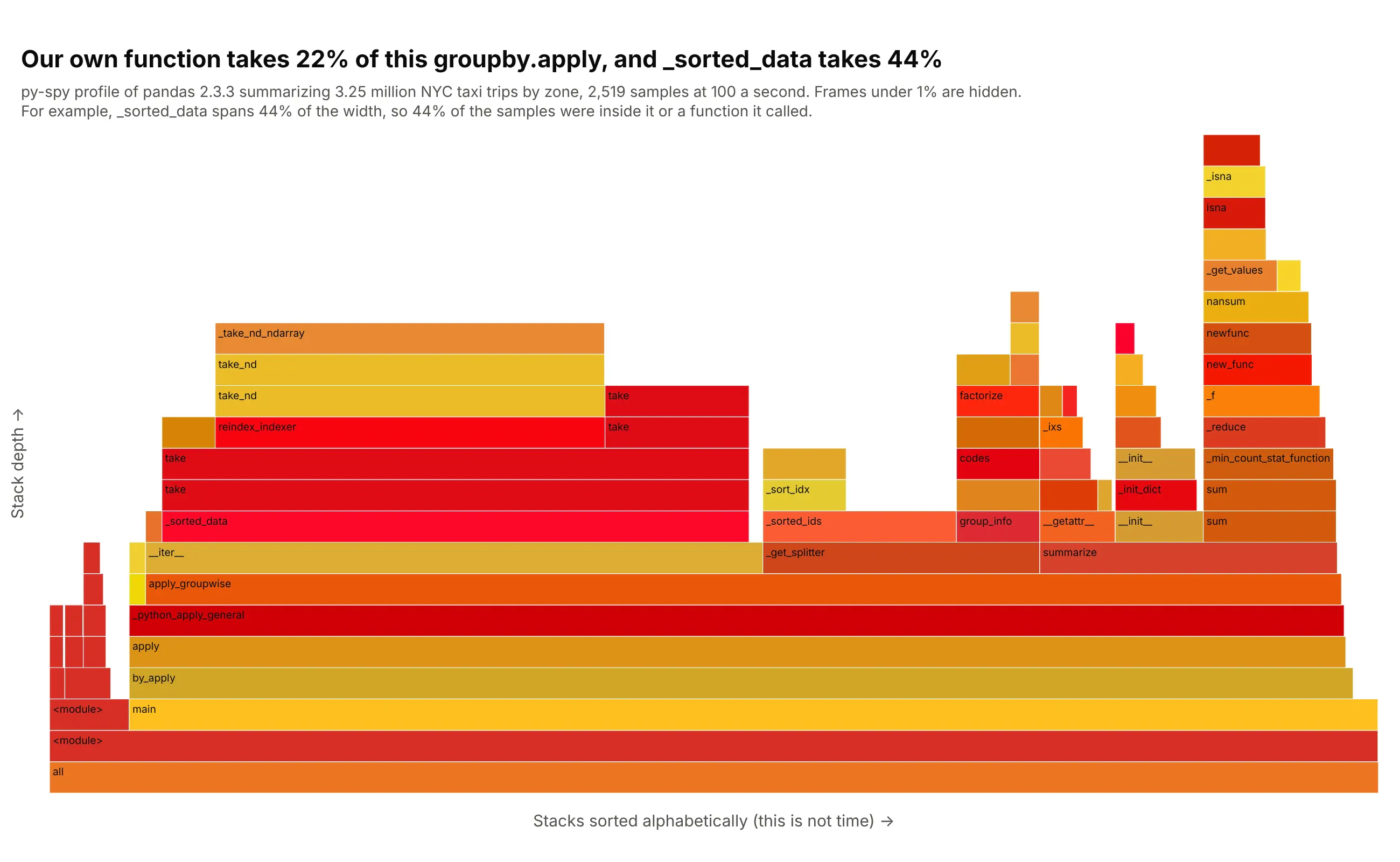
Data: January 2025 yellow taxi trip records from the New York City Taxi and Limousine Commission (TLC), 3,475,226 trips, of which 3,253,864 in 259 pickup zones have a positive distance and fare. The script summarizes fare per mile and tip share by zone with pandas 2.3.3 on Python 3.13, 40 times, and was profiled with py-spy 0.4.2 at 100 samples a second on a shared virtual machine with 4 vCPUs (an Intel Xeon at 2.1 GHz with 15 GB of memory) running Linux 6.18.
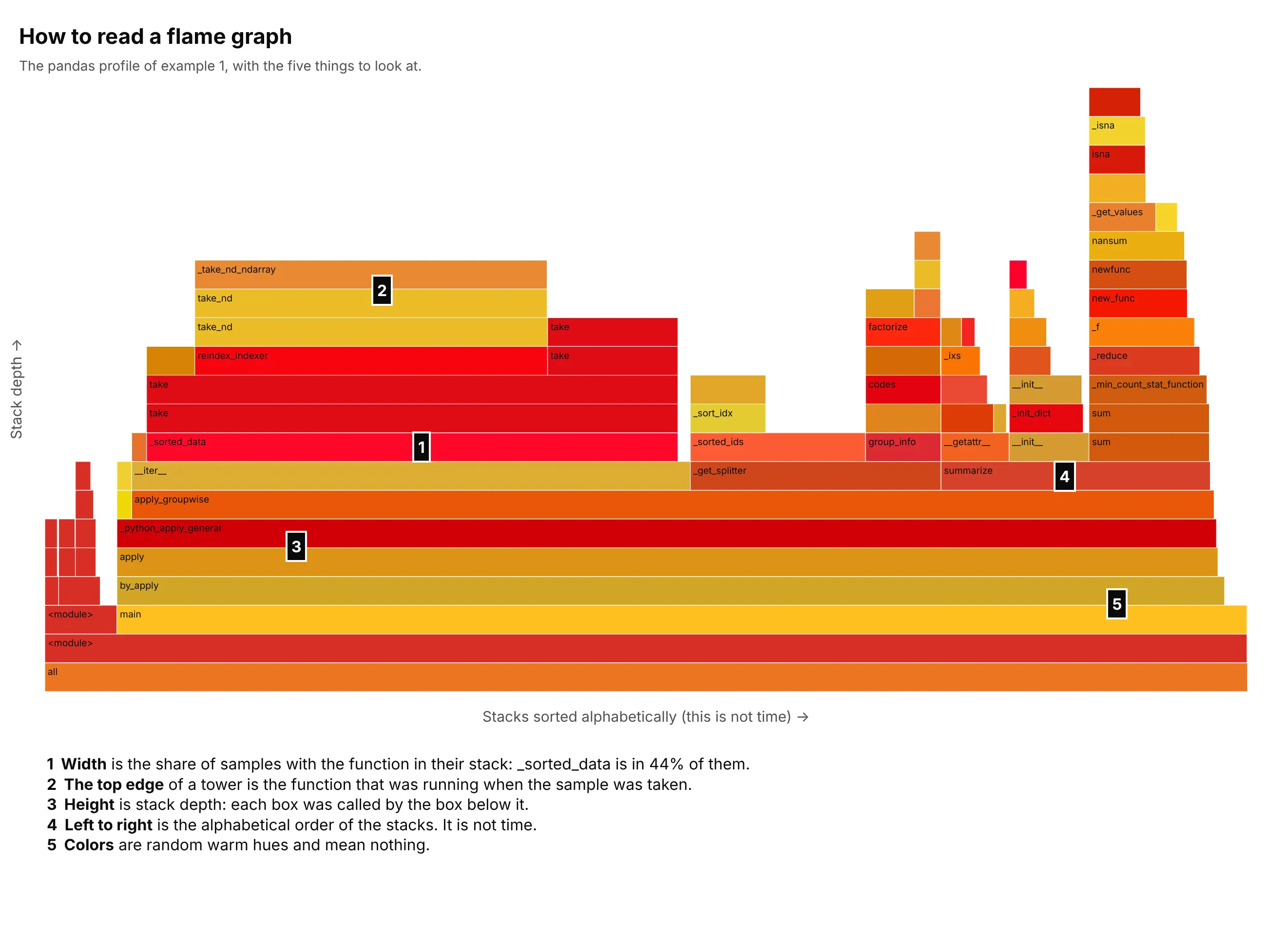
How do you read a flame graph? In the example above, notice these things:
- Each box is one function, drawn on top of the function that called it. The bottom box, all, holds every sample, the next one is the script itself, and the towers above them are calls into pandas. The deepest stack in the data is 21 calls deep.
- Width is the share of samples with that function somewhere in the stack. by_apply holds 2,320 of the 2,519 samples (92%), while reading the Parquet file holds only 23 (0.9%), so the time is in the summary and not in loading the data.
- The function we wrote, summarize, holds 564 samples (22%). _sorted_data holds 1,113 (44%), twice as many, and judging by the take calls above it, it copies the rows into group order before our function runs. This reading comes from the frame names, not from pandas documentation.
- The top edge of a tower is the code that was running when the sample was taken. The tower over _sorted_data ends in _take_nd_ndarray, which tops 738 samples (29%), so that is the plateau worth looking at first.
- Left to right is the alphabetical order of the stacks (__iter__ before _get_splitter before summarize), not the order in which things happened, and the colors are random warm hues that carry no meaning. Frames under 1% of the samples are hidden.
It's often used for charts like these:
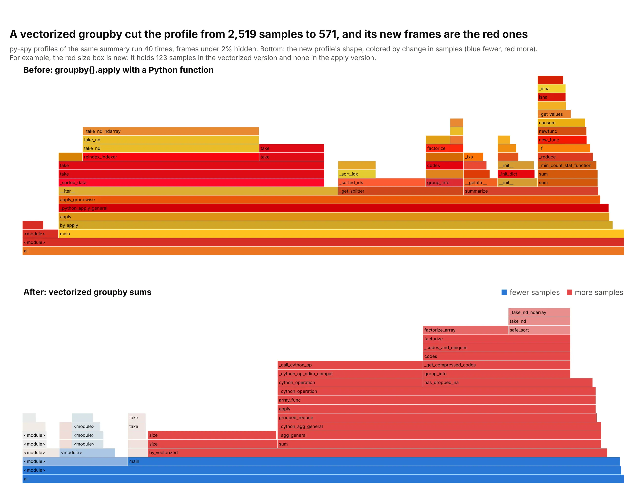
Example 2, a differential flame graph. The same summary written as a vectorized groupby has 571 samples instead of 2,519, and the frames that exist only in the new version (grouped_reduce, size, factorize) are red because they grew from nothing. Data: the same taxi profiles as above, before and after.
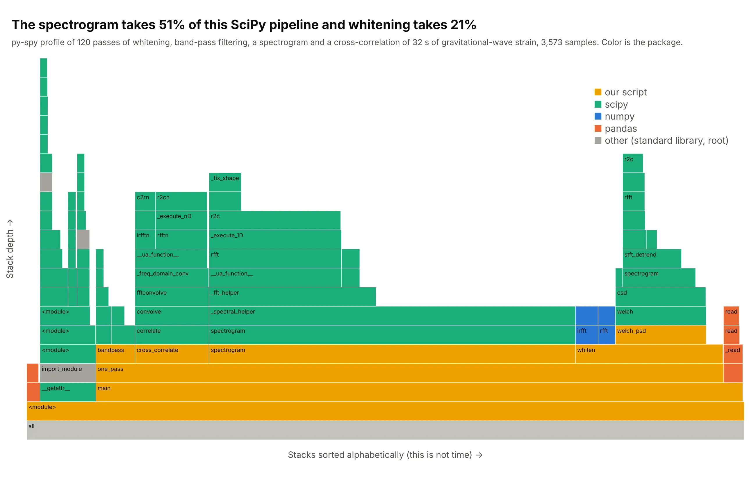
Example 3, scientific code. Coloring by package instead of at random answers "whose code is this" at a glance, and here shows that the spectrogram step is 51% of the time of a SciPy pipeline that processes 32 seconds of LIGO (Laser Interferometer Gravitational-Wave Observatory) strain around the first gravitational wave detection, GW150914. Data: Gravitational Wave Open Science Center, profiled with py-spy over 120 passes.
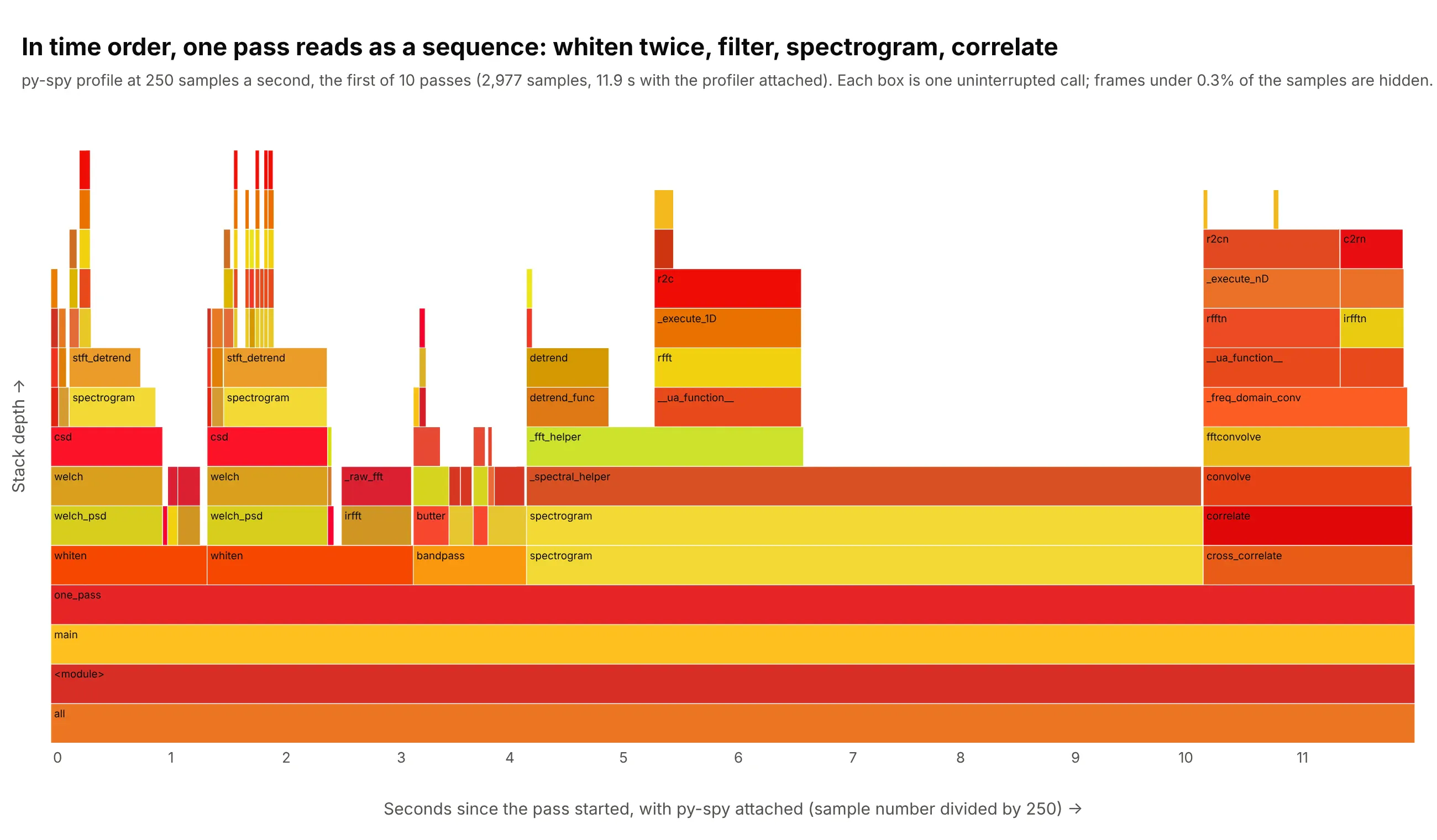
Example 4, a flame chart. With time on the x axis the same pipeline reads as a sequence, with two whitening steps, a filter, the spectrogram and the cross-correlation in order, which a flame graph hides on purpose. Data: the first of 10 passes of the same LIGO pipeline at 250 samples a second.
How to read a flame graph from another field
The chart assumes a few ideas from software performance work, and each of them decides what a box or a width means.
- A call stack is the list of functions that are running at one instant, because a function that is running was called by another function, which was called by another, back to the start of the program. main calls by_apply, which calls apply, and so on down to the function that is executing, which is the top of the stack. A flame graph draws that list from the bottom up.
- A sampling profiler looks at the call stack many times a second and counts what it sees, instead of timing every function (which slows the program and changes what it measures). If a function is in 22% of the samples, the program was running it, or running something it called, about 22% of the time. py-spy samples a Python program from outside, 100 times a second by default, and by default skips threads that are waiting, so the samples describe work and not idle time.
- Folded stacks are the text a profiler writes and a flame graph is drawn from: one line per distinct stack, with the function names joined by semicolons and the number of samples with that stack at the end. An example follows the list.
- Total time and self time are the two ways to count a function. The width of a box is its total, which includes everything it called, and the part of its width that is not covered by boxes above it is its self time. In the graph above, the blank space at the top of summarize is time spent in summarize itself.
- Merging is what makes a flame graph readable. Thousands of samples have only a few hundred distinct stacks (244 in the example), so the picture sorts the stacks alphabetically and joins neighbors that share the same start, which is why identical code paths become one wide box.
This is the tallest tower of the example above as one line of folded stacks, with the file names removed:
<module>;main;by_apply;apply;_python_apply_general;apply_groupwise;__iter__;_sorted_data;take;take;reindex_indexer;take_nd;take_nd;_take_nd_ndarray 738
Here are the five things to look at, numbered on the profile of the main example (example 1):
A short history
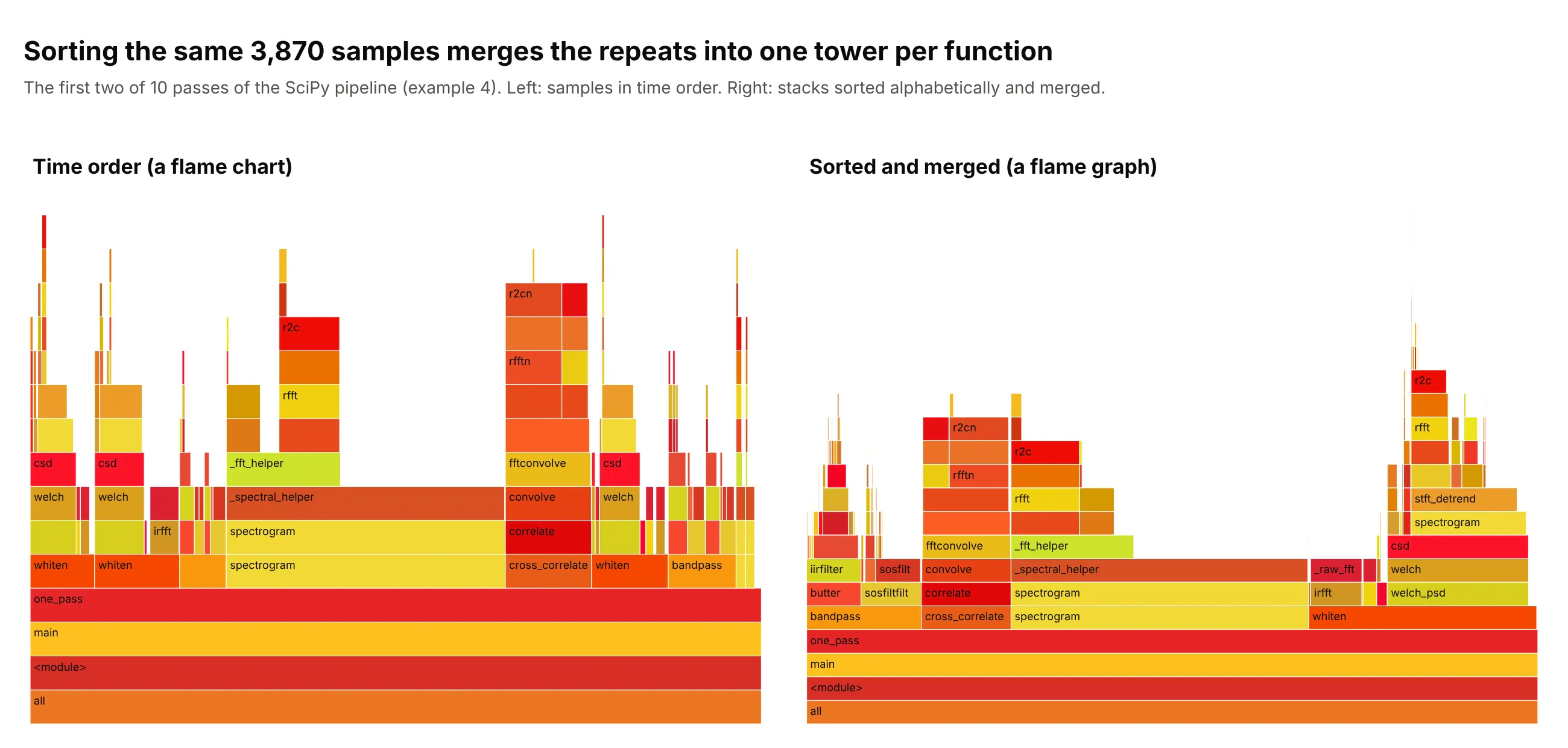
Brendan Gregg invented flame graphs while working on a MySQL performance issue and needed to understand central processing unit (CPU) usage quickly and in depth, because the profilers he had produced walls of text. He released the code in December 2011, and his flame graph page says that the x axis shows the stack profile population sorted alphabetically (it is not the passage of time), that the y axis shows stack depth, and that the original flame graphs use random colors to tell adjacent frames apart. He later settled on warm colors, which is where the name comes from. The page also says that the samples were first drawn in time order and were reordered to maximize frame merging. He described the design in "The Flame Graph" in ACM Queue (the magazine of the Association for Computing Machinery, ACM), which was reprinted in Communications of the ACM 59(6), 2016. In 2014 he added red and blue differential flame graphs, where the shape is that of the second profile and red shows growth and blue a reduction. We don't have his MySQL profile, so this redraws the idea with the SciPy pipeline of example 4, the flame chart: the same samples in time order on the left, and sorted and merged on the right.
Alternatives to a flame graph
Here's the same pandas profile drawn five ways, next to the flame graph. Some are better for the question, some worse, some just different:
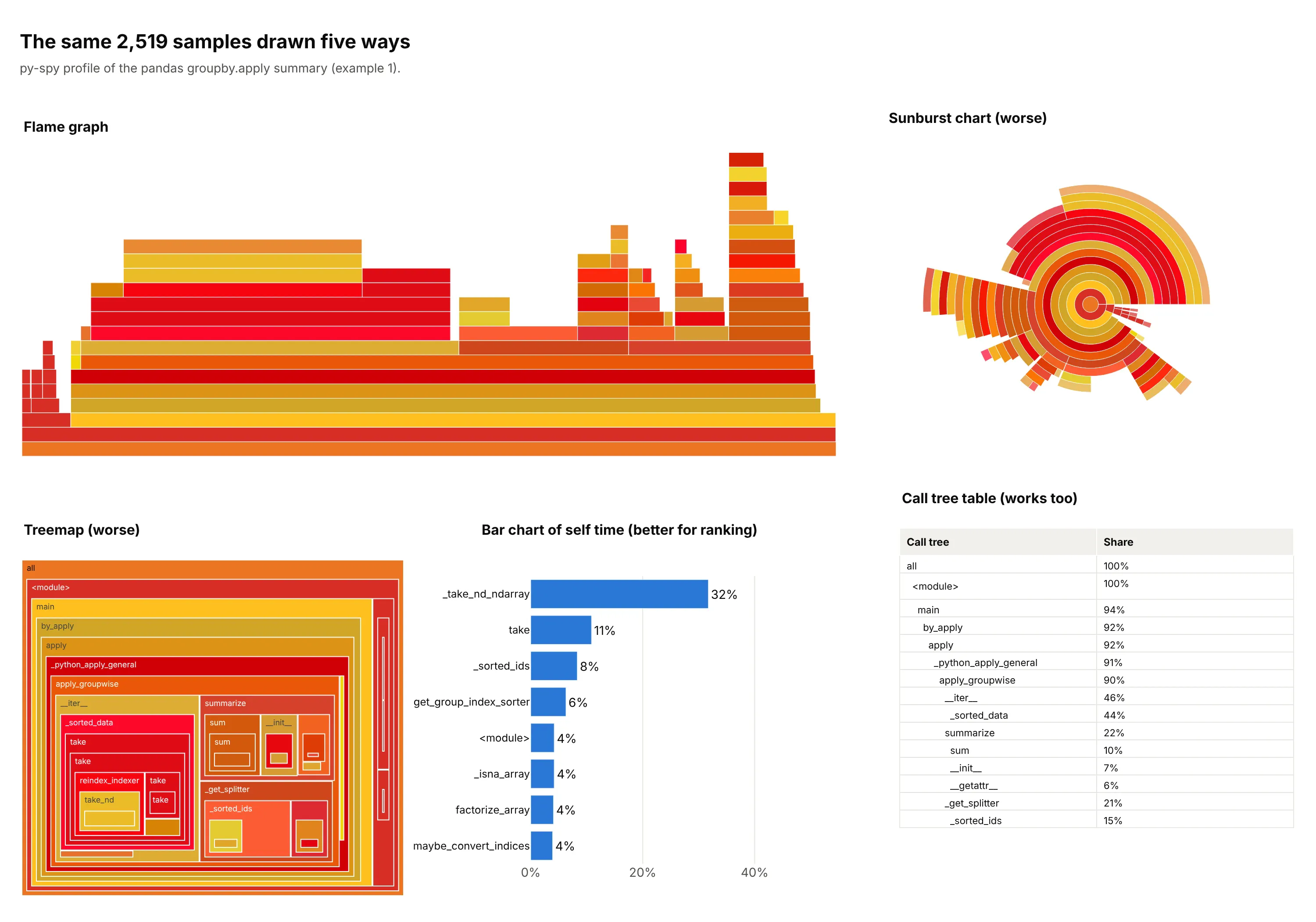
- Sunburst chart (worse). It shows the same hierarchy as rings, but the stack here is 21 levels deep, so the outer rings become slivers, and comparing the angle of two arcs is harder than comparing two widths on a common baseline.
- Treemap (worse). Area shows each function's share, but depth turns into boxes inside boxes, and the call order, the thing you follow in a stack, is lost. A treemap suits hierarchies where the question is "which category is biggest".
- Bar chart of self time (better for ranking). It puts _take_nd_ndarray first with 32% of the samples as its own time, which is the top of the plateau in the flame graph, and it is the quickest way to rank functions. It loses who called them, so you can't tell that the cost comes from _sorted_data.
- Call tree table (works too). A text list of functions with their shares is what profilers such as Python's cProfile print, and it holds exact numbers, but you read many rows to find what the flame graph shows at a glance.
- Flame chart (different). It has time on the x axis, so it answers "what happened when" (example 4 above), and it splits a function that runs several times into several boxes, so it is poor at totals.
- Icicle graph (works too). It is the same chart with the root on top, which many tools use because the entry point stays visible without scrolling (example 5 below). The icicle chart guide covers the chart type in general.
How to make a flame graph
With AI
ChatGPT, Claude Code, GitHub Copilot, Cursor and other AI tools are excellent at writing Plotly code. Name Plotly in the prompt, and say how the stacks are stored and how the boxes are ordered and colored:
Make a plotly flame graph from profile.txt (py-spy raw output: one call stack per line, frames joined by ";",then a space and the sample count).- Build a tree with an "all" root, merge identical stacks and sum the samples of every prefix.- Draw it with go.Icicle (ids, parents, labels, values, branchvalues="total", sort=False,tiling=dict(orientation="v", flip="y")) so the root is at the bottom.- Order siblings alphabetically (this is not time) and hide frames under 1% of all samples.- Color every function with a random warm color (red, orange, yellow) seeded by its name.- Hover shows the function, its sample count and its share. A title that states the takeaway, and a subtitle withthe profiler, the sampling rate and the number of samples.
With Plotly Studio
Plotly Studio is a product for creating data visualizations and Dash apps and for analyzing data with AI, available as a desktop app or embedded in Dash apps. Ask for a flame graph the same way:
Show a flame graph of this py-spy profile, with the root at the bottom and frames sorted alphabetically, a search box that highlights every frame whose name matches, and a slider for the smallest frame to draw.
Make a flame graph in Python or JavaScript
This is the code AI tools write under the hood. First record a profile. py-spy record -f raw -o profile.txt -- python your_script.py runs your script and writes the folded stacks, and the function below turns them into a flame graph with go.Icicle. flip="y" puts the root at the bottom, and sort=False keeps the alphabetical order the code sets:
import hashlibimport plotly.graph_objects as godef warm(name):"""Brendan Gregg's random warm palette, seeded by the function name so it keeps its color."""h = hashlib.md5(name.encode()).digest()return f"rgb({205 + h[0] * 50 // 255},{h[1] * 230 // 255},{h[2] * 55 // 255})"def flame_graph(folded_path, min_share=0.01):"""Flame graph from py-spy raw output: one stack per line, frames joined by ";", then a sample count."""totals = {}for line in open(folded_path):stack, n = line.rsplit(" ", 1)frames = ["all"] + [f for f in stack.split(";") if "<frozen" not in f]for i in range(1, len(frames) + 1):path = tuple(frames[:i])totals[path] = totals.get(path, 0) + int(n)keep = [p for p, v in totals.items() if v >= min_share * totals[("all",)]]keep.sort(key=lambda p: [f.lower() for f in p]) # siblings in alphabetical orderreturn go.Figure(go.Icicle(ids=[";".join(p) for p in keep], parents=[";".join(p[:-1]) for p in keep],labels=[p[-1].split(" (")[0] for p in keep], values=[totals[p] for p in keep],branchvalues="total", sort=False, tiling=dict(orientation="v", flip="y"),marker=dict(colors=[warm(p[-1]) for p in keep], line=dict(width=0.6, color="white")), root_color="white",pathbar=dict(visible=False), hovertemplate="%{label}: %{value} samples (%{percentRoot:.1%})<extra></extra>"))flame_graph("profile.txt").show()
In JavaScript, plotly.js draws the same chart from an icicle trace. This example builds the tree from a few folded stacks (the biggest frames of the profile in example 1 collapsed to six rows) and draws the same chart:
<div id="chart"></div><script src="https://cdn.plot.ly/plotly-4.1.1.min.js"></script><script>// Folded stacks: frames joined by ";", then the number of samples with that stack at the top.// These are the biggest frames of the pandas groupby.apply profile above, collapsed to a few rows.const folded = [["main;by_apply;apply;apply_groupwise;__iter__;_sorted_data", 1113],["main;by_apply;apply;apply_groupwise;__iter__", 57],["main;by_apply;apply;apply_groupwise;_get_splitter", 525],["main;by_apply;apply;apply_groupwise;summarize", 564],["main;by_apply;apply;apply_groupwise", 8],["main;read_parquet", 23]];const totals = new Map();for (const [stack, n] of folded) {const frames = ["all", ...stack.split(";")];for (let i = 1; i <= frames.length; i++) {const id = frames.slice(0, i).join(";");totals.set(id, (totals.get(id) || 0) + n);}}const ids = [...totals.keys()].sort((a, b) => a.toLowerCase() < b.toLowerCase() ? -1 : 1); // siblings in alphabetical orderconst name = id => id.split(";").pop();// Random-looking warm colors (reds, oranges, yellows) that depend only on the name, so they carry no meaning.const hash = s => [...s].reduce((h, c) => (h * 31 + c.charCodeAt(0)) >>> 0, 7);const warm = s => { const h = hash(s); return `rgb(${205 + h % 51},${(h >> 8) % 231},${(h >> 16) % 56})`; };Plotly.newPlot("chart", [{type: "icicle", ids, labels: ids.map(name), parents: ids.map(id => id.includes(";") ? id.slice(0, id.lastIndexOf(";")) : ""),values: ids.map(id => totals.get(id)), branchvalues: "total", sort: false,tiling: {orientation: "v", flip: "y"}, root_color: "white", pathbar: {visible: false},marker: {colors: ids.map(id => warm(name(id))), line: {width: 0.6, color: "white"}},hovertemplate: "%{label}: %{value} samples (%{percentRoot:.1%})<extra></extra>"}], {width: 900, height: 480, margin: {t: 30, l: 10, r: 10, b: 10}, title: {text: "Where the time goes"}});</script>
The Python output of py-spy is also the input of Gregg's own flamegraph.pl, which writes an interactive SVG (scalable vector graphics) file, so you can compare the two. For a differential graph, subtract the sample counts of the two profiles stack by stack and color each box by the change, as example 2 does.
Share it
Every Plotly chart has a Share chart button (the cloud icon in its toolbar) that uploads it to Plotly Cloud and gives you a link. Only you can see it until you change its visibility.
For a live app, put the chart in a Dash app and publish it with the Plotly Cloud command-line interface (CLI). Coding agents can run these commands for you:
pip install "dash[cloud]"plotly user loginplotly app publish
If your data has to stay in your own cloud or data center, publish to Dash Enterprise instead.
Dos and don'ts
A flame graph is read by width, so most of the work is keeping the picture honest about what the axes are and keeping slivers and long labels from hiding the wide boxes. Here is the pandas profile both ways, in the same colors.
Don't label the x axis as time, keep every frame down to a single sample so hairline slivers fill the plot, print each frame as "name (path/file.py)" so labels run past their boxes, or use a default serif font:
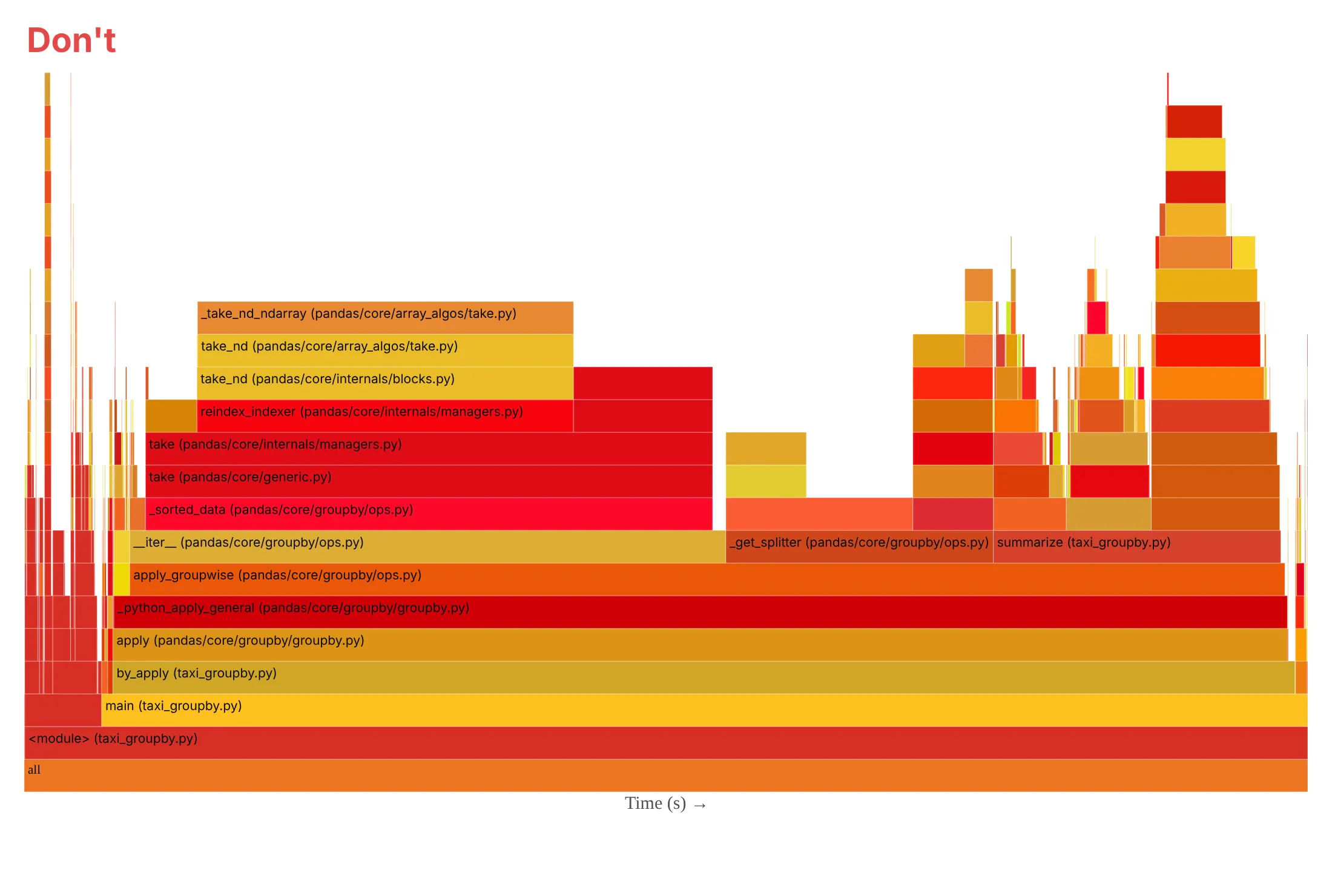
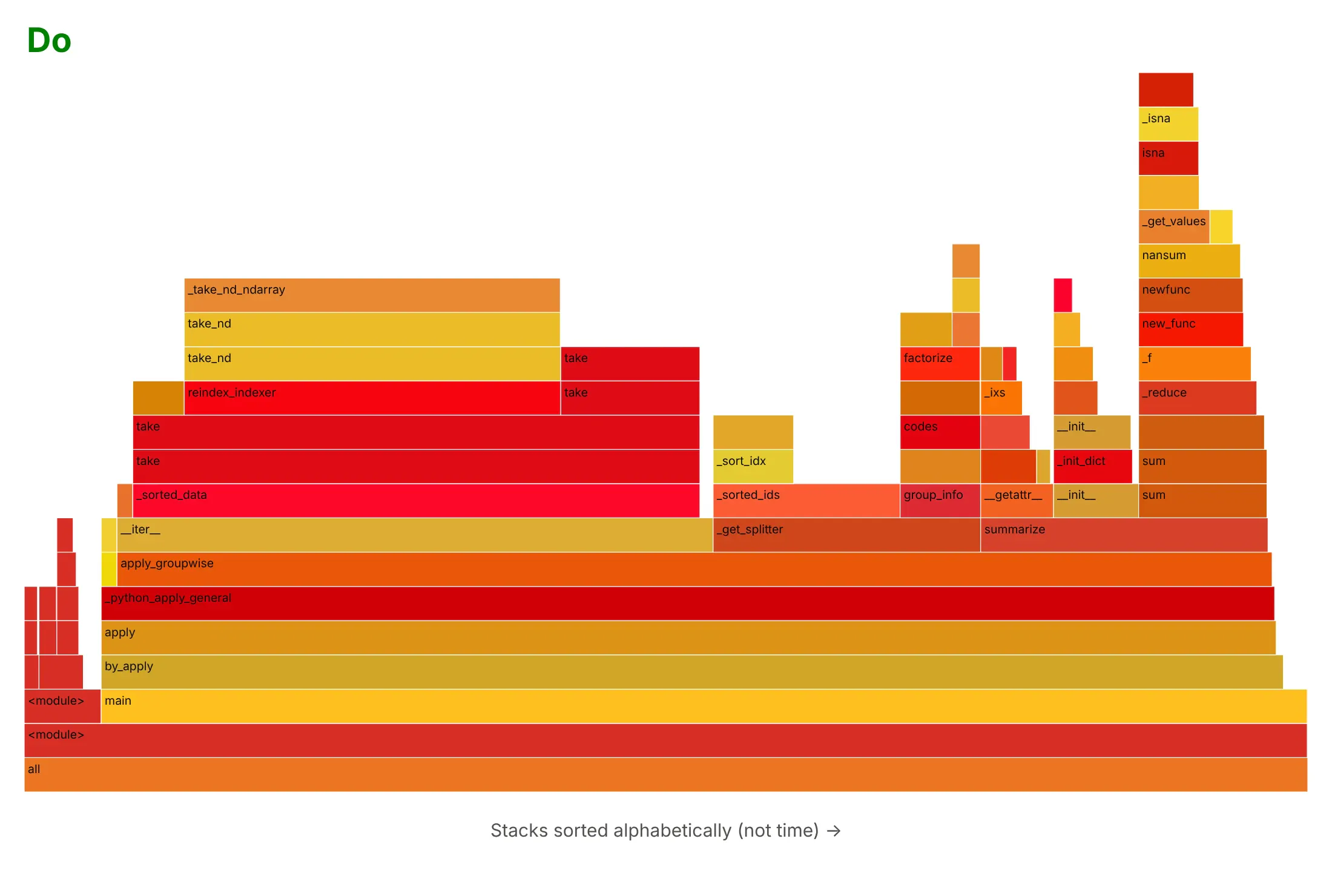
Do say that the x axis is the alphabetical order of the stacks, hide frames under 1% of the samples, label boxes with the function name and put the file in the hover text, and use one sans-serif font. Reading a box in words helps too: here _sorted_data spans 44% of the width, so 44% of the samples were inside it or a function it called.
Checklist
Do
- Merge identical stacks and sort siblings alphabetically, which is what makes the boxes wide enough to read.
- Say how the profile was recorded: the tool, the sampling rate, how long the program ran, how many samples there are and what the machine was.
- Record several thousand samples, because the shares of small boxes are rough (example 7 below).
- Use random warm colors, or one color per package with a key. Keep red and blue for differences between two profiles.
- Use the same ordering and the same sample counts when you compare two profiles.
Don't
- Read the x axis as time, or the order of the towers as the order of events. A flame chart is the one with time.
- Read colors as meaning "hot" or "slow". The warm hues are random.
- Trust a frame with a few dozen samples. Ten samples more or fewer would change its width.
- Forget what the profiler can't see. py-spy samples Python frames, so NumPy and other native code appears as the self time of the Python function that called it.
More flame graph examples
Four more flame graphs built from real profiles, each with its data, a tip and a prompt to rebuild it.
5. An icicle graph of plotly.py
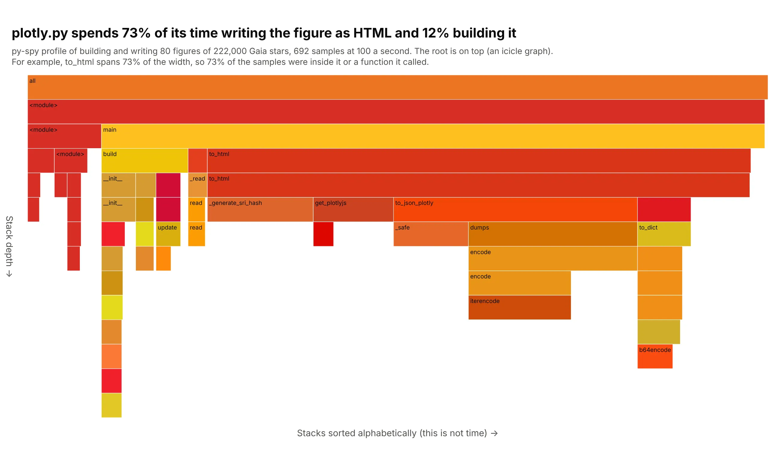
Writing the figure as HTML takes 508 of the 692 samples (73%), while building it takes 81 (12%). Inside to_html, converting the figure to JSON is the widest part (to_json_plotly, 33%), and _generate_sri_hash takes 99 samples (14%), which by its name is the checksum for the script tag. The root is on top, which is how many profilers draw the same data. Data: Gaia Data Release 3 stars within 100 parsecs (222,000 stars, from the Hertzsprung-Russell diagram guide), 80 repeats of building a go.Scatter figure and calling fig.to_html, profiled with py-spy.
Tip: use the root-on-top layout when the entry point or long function names matter more than the flame look, and say which direction the stack grows.
Get the data from a py-spy profile (py-spy record -f raw -o profile.txt -- python script.py at 100 samples a second)of a script that reads the Gaia DR3 stars within 100 parsecs (columns bp_rp, abs_g) and 80 times builds a plotlygo.Scatter figure and calls fig.to_html(include_plotlyjs="cdn").Build a tree from the folded stacks and draw it with plotly go.Icicle with the root at the top (no flip),siblings in alphabetical order, random warm colors seeded by the function name, frames under 1.5% hidden, anda title that gives the share of samples under to_html.
6. Searching for a library across the graph
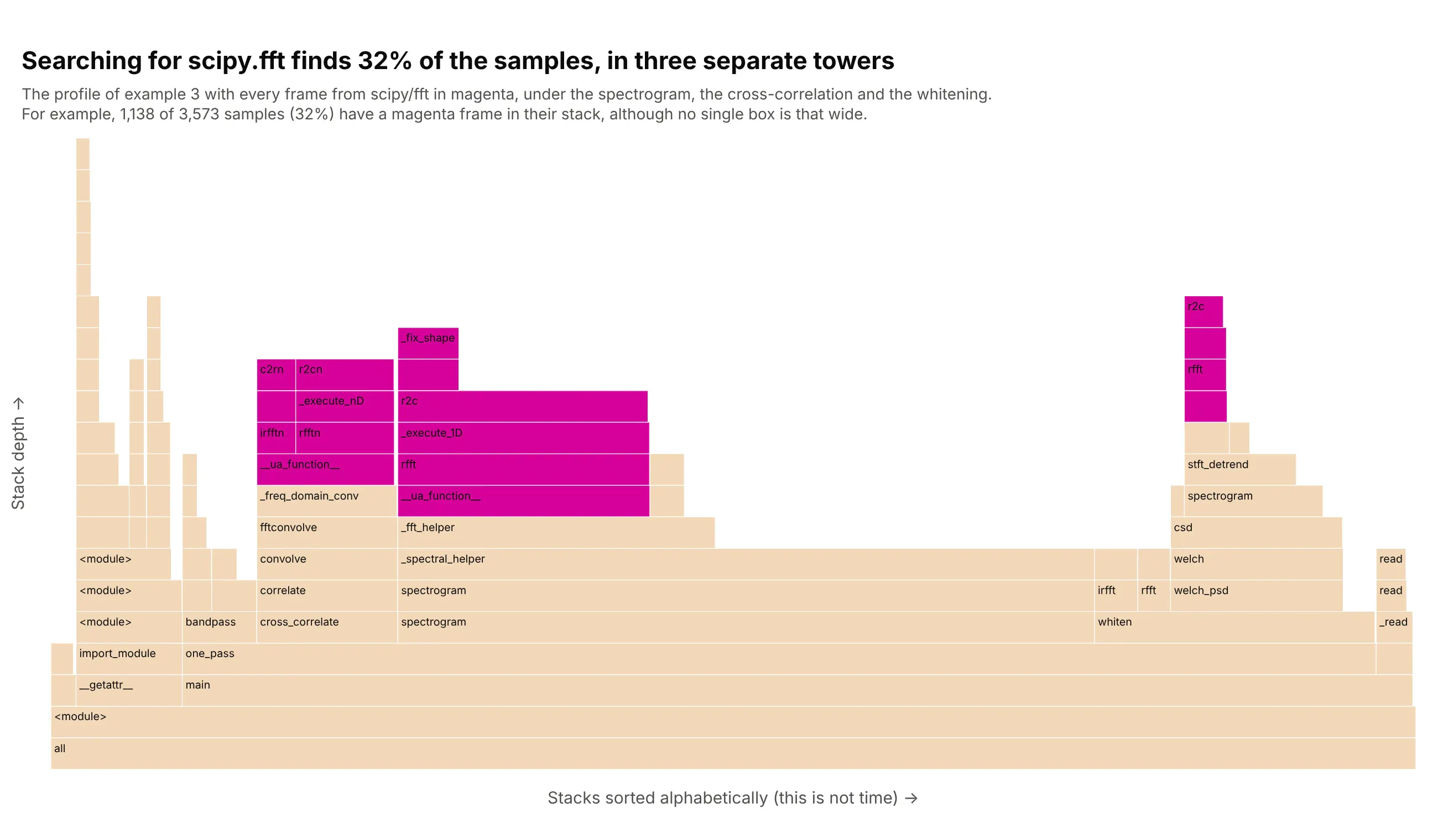
A library that is called from several places is split across several towers, and the only way to see its total is to highlight it. Every frame from scipy/fft is magenta here, in three towers under the spectrogram, the cross-correlation and the whitening, and together 1,138 of 3,573 samples (32%) have one of those frames in their stack. Gregg's flame graph SVGs have a search box that does this and shows the share of stacks that match. Data: the LIGO SciPy profile of example 3.
Tip: count a sample once even when several matching frames are in its stack, or recursive functions add up to more than 100%.
Get the data from the Gravitational Wave Open Science Center: the 32 s of strain around GW150914 from the Hanfordand Livingston detectors (H-H1_LOSC_4_V2-1126259446-32.hdf5 and L-L1_LOSC_4_V2-1126259446-32.hdf5, 4,096 Hz).Write a script that whitens the strain with a Welch noise estimate, band-passes it from 30 to 400 Hz,computes a scipy.signal.spectrogram and cross-correlates the two detectors, repeated 120 times, and profile it withpy-spy at 100 samples a second. Draw a plotly go.Icicle flame graph (root at the bottom, siblings alphabetical)with every frame from scipy/fft in magenta and the rest pale, and report the share of samples with a match.
7. How much a profile changes from run to run
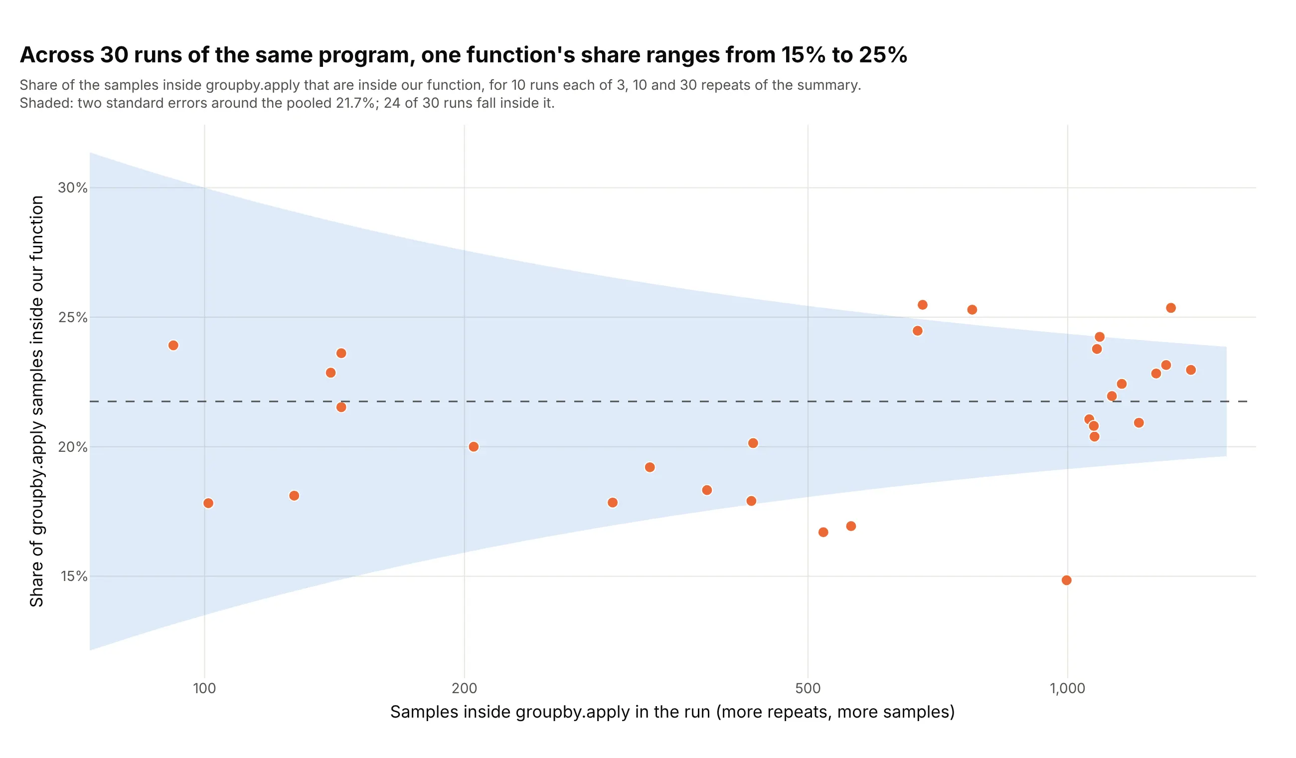
A profiler counts a few hundred or a few thousand snapshots, so every width has a sampling error. In 30 runs of the same program the share of groupby.apply that sits in our function runs from 15% to 25% (pooled 21.7%). A share p from n independent samples has a standard error of the square root of p(1 - p)/n, and 24 of the 30 runs fall within two of them. That is fewer than the 28 or 29 expected from sampling alone, and we did not test why (the machine was shared with other jobs, and consecutive samples are not independent, which is our reading). Data: py-spy runs of the taxi workload with 3, 10 and 30 repeats, 10 runs each, 206 to 1,169 samples on average.
Tip: print the sample count on every flame graph and treat differences of a few percentage points between two profiles as noise unless you have repeated the run.
Get the data from a table of 30 py-spy runs (columns repeats, run, apply_samples, summarize_samples: the samplesinside groupby.apply and the samples of those inside our summarize function).Build a plotly scatter of apply_samples (log x axis) against summarize_samples / apply_samples, one dot per run,a dashed line at the pooled share, and a shaded band of two standard errors, 2 * sqrt(p * (1 - p) / n), around it.
8. Zooming into one function
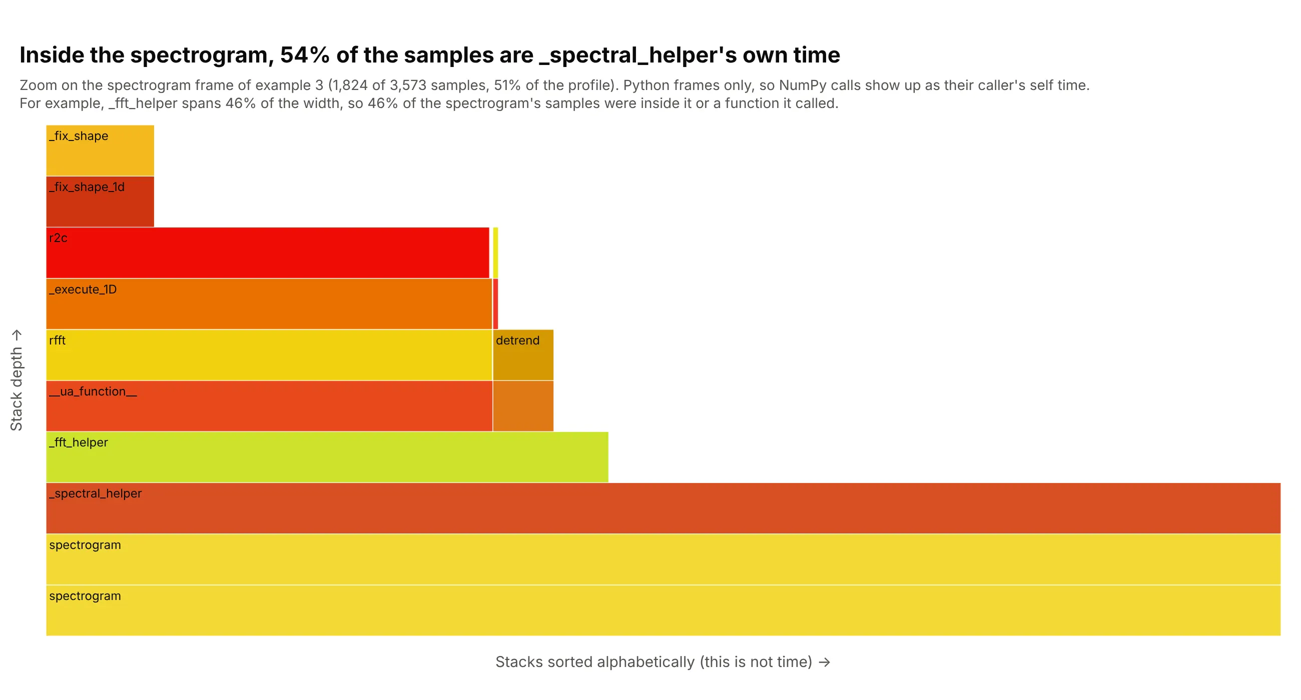
Clicking a frame makes it the full width, so a function that is 51% of the profile gets enough pixels to read. Inside the spectrogram, _fft_helper is 831 of 1,824 samples (46%), and the FFT (fast Fourier transform) call r2c is 655 (36%). The other 992 samples (54%) are the self time of _spectral_helper, where NumPy calls run in compiled code with no Python frames, so they show up as time in their caller. In Plotly the zoom is the level of the icicle trace, or a click on a box. Data: the LIGO SciPy profile of example 3.
Tip: set level to the id of the frame to zoom on and keep the root's path in the subtitle, so readers know the widths are now relative to that frame.
Get the data from a py-spy profile of the scipy.signal pipeline of the previous example (folded stacks, one line perstack with a sample count, 3,573 samples).Build a plotly go.Icicle flame graph (root at the bottom) with level set to the id of the spectrogram frame, so thatframe fills the width, and a subtitle that says how many samples and what share of the whole profile it holds.
FAQ
Options to customize
These are the go.Icicle options that matter most for flame graphs, see the reference for the full list.
- ids, parents, values: the tree. Use one id per distinct stack prefix (the frames joined by ;), the id of the prefix without the last frame as the parent, and the sample count as the value.
- branchvalues="total": says that a parent's value already includes its children, which is true of samples. The part of a parent not covered by children is its self time, shown as blank space.
- tiling.orientation and tiling.flip: orientation="v" lays the levels out as rows, and flip="y" puts the root at the bottom for a flame graph. Leave flip out for an icicle graph.
- sort=False: keeps the order of your input, so you control the order of siblings (alphabetical for a flame graph, time for a flame chart).
- marker.colors: one color per frame. Use random warm hues for the classic look, one color per package, or a diverging scale for a differential flame graph, with marker.cmin and marker.cmax to set the range.
- marker.line: the border of each box. A thin white line (0.5 to 1 px) separates adjacent frames without hiding narrow ones.
- level: the id of the frame to show as the root, which is how you zoom into one function.
- maxdepth: the number of levels to draw below the root, which keeps very deep stacks readable.
- pathbar.visible: set it to False to hide the breadcrumb bar a flame graph doesn't need.
- root_color: the color of the root box when it has none of its own, set to white to make it blend with the page.
- text and hoverinfo or hovertemplate: what shows on hover, such as the function, its sample count and its share of the root (%{percentRoot}), and the file name that you left out of the label.
- insidetextfont and the layout's uniformtext: the label size, and whether labels that don't fit are hidden (uniformtext=dict(minsize=9, mode="hide")).