
Chris Parmer
November 18, 2026
Correlation Matrix Plots - A Complete Guide
TL;DR
- A correlation matrix plot draws the correlation coefficient of every pair of variables as a grid of colored cells, where the coefficient runs from -1 (one variable falls as the other rises) through 0 (no straight-line relationship) to 1 (they rise and fall together), so you can scan dozens of variables for the groups that move together.
- Correlation matrix plots are also known as correlograms, corrgrams and correlation heatmaps, and are similar to heatmaps, scatter plot matrices and dendrograms.
- Four conventions make one readable: a diverging color scale fixed from -1 to 1 with white at 0, only the lower triangle because the matrix is symmetric, the coefficient printed in each cell, and rows ordered by hierarchical clustering so related variables sit together.
- A coefficient summarizes one kind of relationship (a straight line for Pearson, a rising or falling trend for Spearman), so check outliers, curves, small samples and shared drivers before reading it as more, and never read it as proof that one variable causes another.
- You can make one with Plotly in Python or JavaScript, in one line for the basic version: px.imshow(df.corr(), zmin=-1, zmax=1, color_continuous_scale="RdBu_r").
What is a correlation matrix plot?
This is a correlation matrix plot:
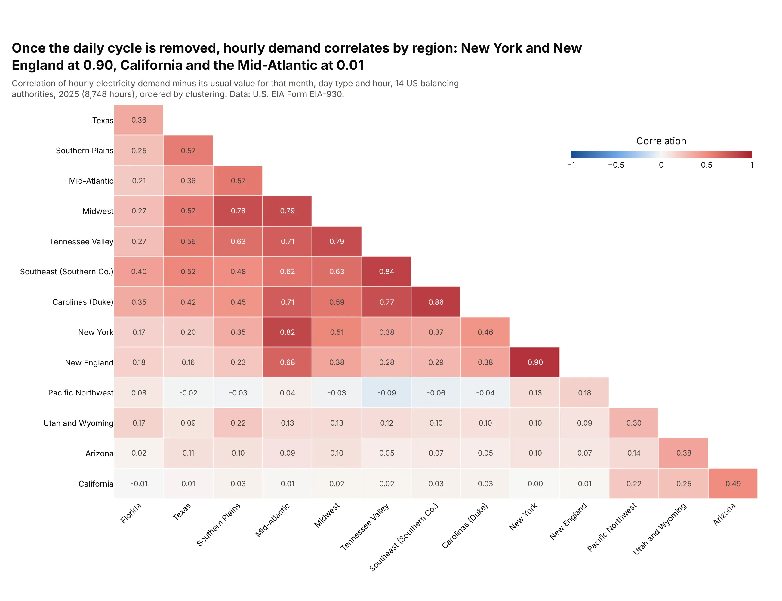
Data: U.S. Energy Information Administration (EIA), Form EIA-930, hourly demand of 14 balancing authorities in 2025.
How do you read a correlation matrix plot? In the example above, notice these things:
- Each cell is one pair of balancing authorities, the operators that keep supply and demand matched in one part of the power grid, and its color and number are the correlation of their hourly electricity demand, so red means demand was above its usual level in both at the same time.
- The demand was first reduced to its deviation from the usual value for that month, day type (weekday or weekend) and hour of the day, because raw demand in every region rises and falls with the same daily and seasonal rhythm (example 4 below shows the difference). What is left is mostly weather and events.
- The color scale is fixed from -1 to 1 with white at 0, so a pale cell means almost no relationship, and the same color means the same thing in every matrix in this guide. These 91 pairs run from -0.09 to 0.90, with a median of 0.22.
- Only the lower triangle is drawn, because the correlation of A with B equals the correlation of B with A, and the diagonal is always 1, so every pair appears once.
- The rows are ordered by clustering, which brings the strong pairs together: New York and New England at 0.90, the Southeast and Duke's Carolinas at 0.86, the Midwest, the Mid-Atlantic and Tennessee Valley in a red block of 0.71 to 0.79, and California, which is near 0.01 with the Mid-Atlantic and only 0.49 with its neighbor Arizona.
It's often used for charts like these:
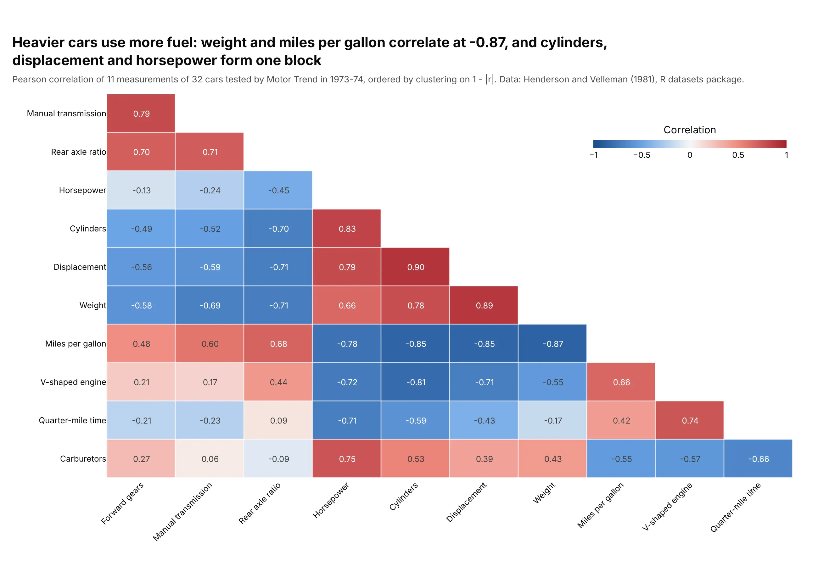
The classic textbook table. The 32 cars of the R mtcars table give 55 pairs, and heavier cars have lower mileage (r = -0.87) while cylinders, displacement and horsepower form one block of 0.79 to 0.90. Data: Motor Trend road tests, Henderson and Velleman (1981) via the R datasets package.
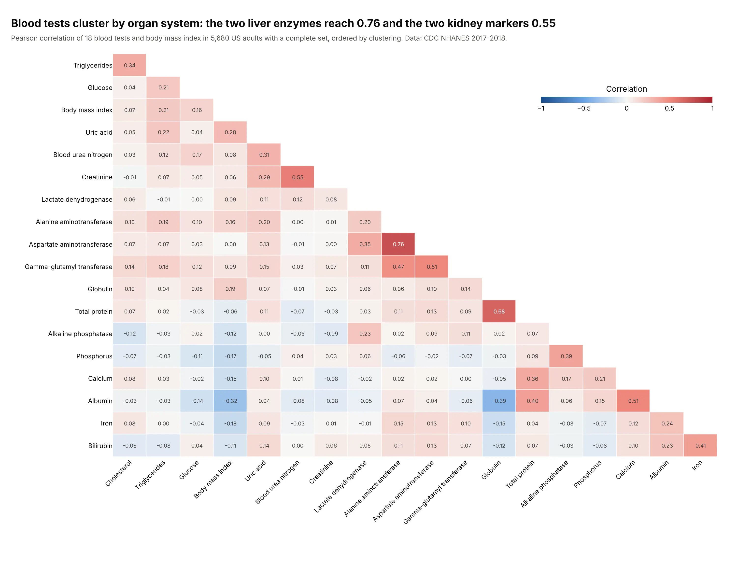
A clinical lab panel. Of the 171 pairs among 18 blood tests and body mass index in 5,680 US adults, only 5 exceed 0.5 in absolute value, and they include the two liver enzymes (0.76), alanine aminotransferase and aspartate aminotransferase. Data: U.S. Centers for Disease Control and Prevention (CDC), National Health and Nutrition Examination Survey (NHANES) 2017-2018.
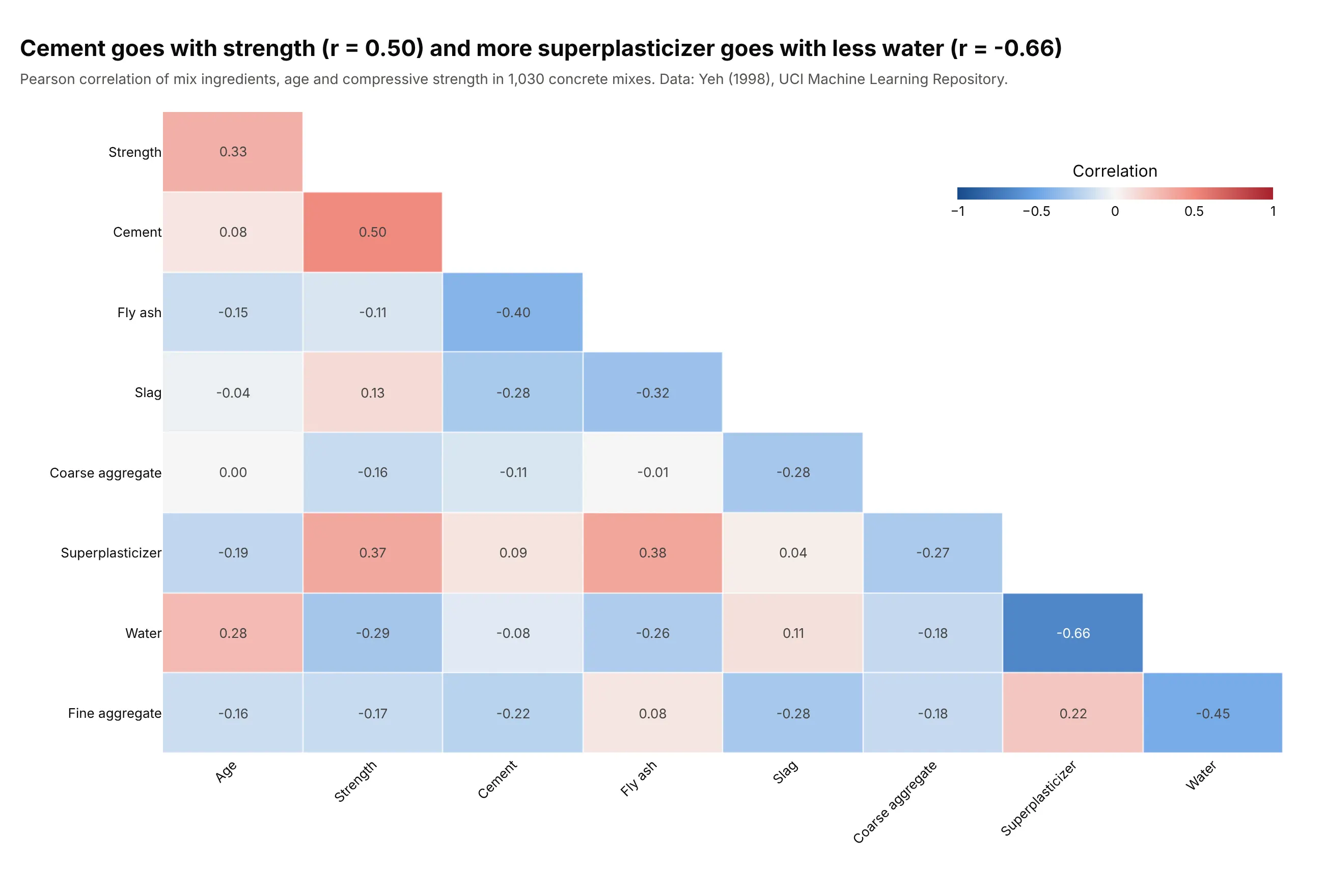
Materials properties. For 1,030 laboratory concrete mixes, cement content has the strongest correlation with compressive strength (0.50), and superplasticizer goes with less water (-0.66), a pattern consistent with superplasticizers being added to cut the water a mix needs. Data: Yeh (1998), UCI Machine Learning Repository.
A short history
Francis Galton introduced the idea of "co-relation" in an 1888 paper on body measurements (Galton 1888, published in 1889), and Karl Pearson worked out the product-moment formula still used today in 1896. Charles Spearman proposed the rank version in 1904. Drawing a whole matrix of coefficients as shapes came much later: Murdoch and Chow (1996) used ellipses, and Friendly (2002) named the result a corrgram, with shaded cells or pie glyphs, ordered so that similar variables sit together. Here is the idea redrawn with the mtcars data:
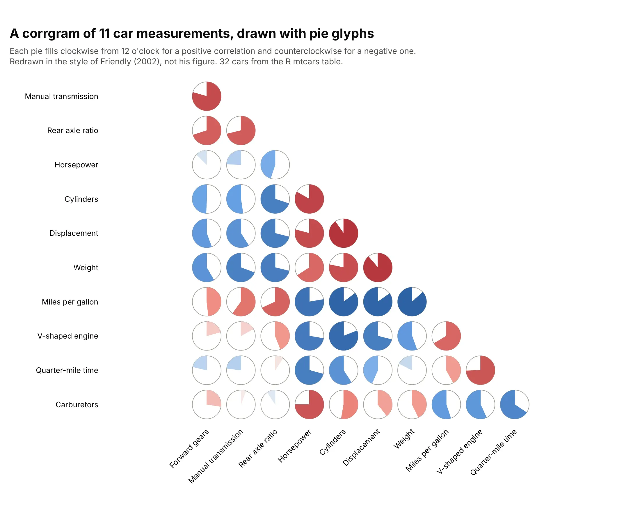
The idea of ordering rows and columns so that groups appear is older still, and the history of the cluster heat map by Wilkinson and Friendly traces it to the 1800s.
What the numbers mean
A correlation matrix plot hides the arithmetic behind its colors, and three parts of it decide whether a plot can be trusted: how the coefficient is calculated, how the rows are ordered, and how much a coefficient from a small sample can be believed.
Pearson, Spearman and Kendall
The Pearson correlation coefficient (r) divides how much two variables vary together, their covariance, by the product of how much each varies on its own, their standard deviations. Dividing removes the units, so r always lies between -1 and 1, and the square of r is the share of one variable's variation that a straight line through the other accounts for. In the car data, weight and miles per gallon have r = -0.87, so r squared is 0.75, and a straight line explains about three quarters of the variation in mileage.
The Spearman correlation coefficient replaces every value by its rank (1 for the smallest, 2 for the next) and then calculates Pearson's r on the ranks. It asks whether one variable tends to rise when the other does, however curved the relationship, and a few extreme values can no longer dominate it. Kendall's tau also uses ranks, by comparing every pair of observations and counting how many agree in order against how many disagree, and it is often preferred for small samples. In pandas, df.corr(method="spearman") and method="kendall" switch between them. Example 2 below shows a pair where Pearson says 0.09 and Spearman says 0.32.
There is no universal cutoff for a strong correlation. Among the blood tests above a value of 0.55 is high, and for the 11 stock sectors in 2019 the average pair was 0.50, so judge a coefficient against what is typical in the field and the data.
How the rows are ordered
Variables in file order or alphabetical order hide structure, so most correlation matrix plots reorder them with hierarchical clustering. The method starts with every variable on its own, repeatedly merges the two closest variables or groups, and stops when one group is left, which gives the tree shown in a dendrogram. The distance between two variables is 1 minus their correlation, so highly correlated variables are close. Using 1 minus the absolute value of the correlation treats a strong negative correlation as close too, which puts weight next to miles per gallon in the car matrix instead of at opposite ends. The distance between two groups is the average of the distances between their members (average linkage), and an optimal leaf ordering step then chooses, among the orders the tree allows, the one in which neighboring rows are the most similar. The examples in this guide use that recipe.
Significance and sample size
A coefficient calculated from n observations carries uncertainty. A p-value gives the probability of seeing a coefficient at least this far from 0 if the two variables were unrelated, and for Pearson's r it comes from a t statistic, r times the square root of (n - 2) divided by (1 - r squared). With 12 observations a correlation must exceed 0.58 in absolute value to be significant at the usual 0.05 level, and with 40 it must exceed 0.31.
A matrix runs many tests at once. With 66 pairs, about three would pass a 0.05 test by chance alone if none of them were truly related, so matrices that mark significance use a multiple-testing correction. Holm's method is a common one, and it orders the p-values from smallest to largest and tightens the threshold for each. Example 3 below shows what survives.
Alternatives to a correlation matrix plot
Here's the same car data drawn six ways. Some are better for the question, some worse, some just different:
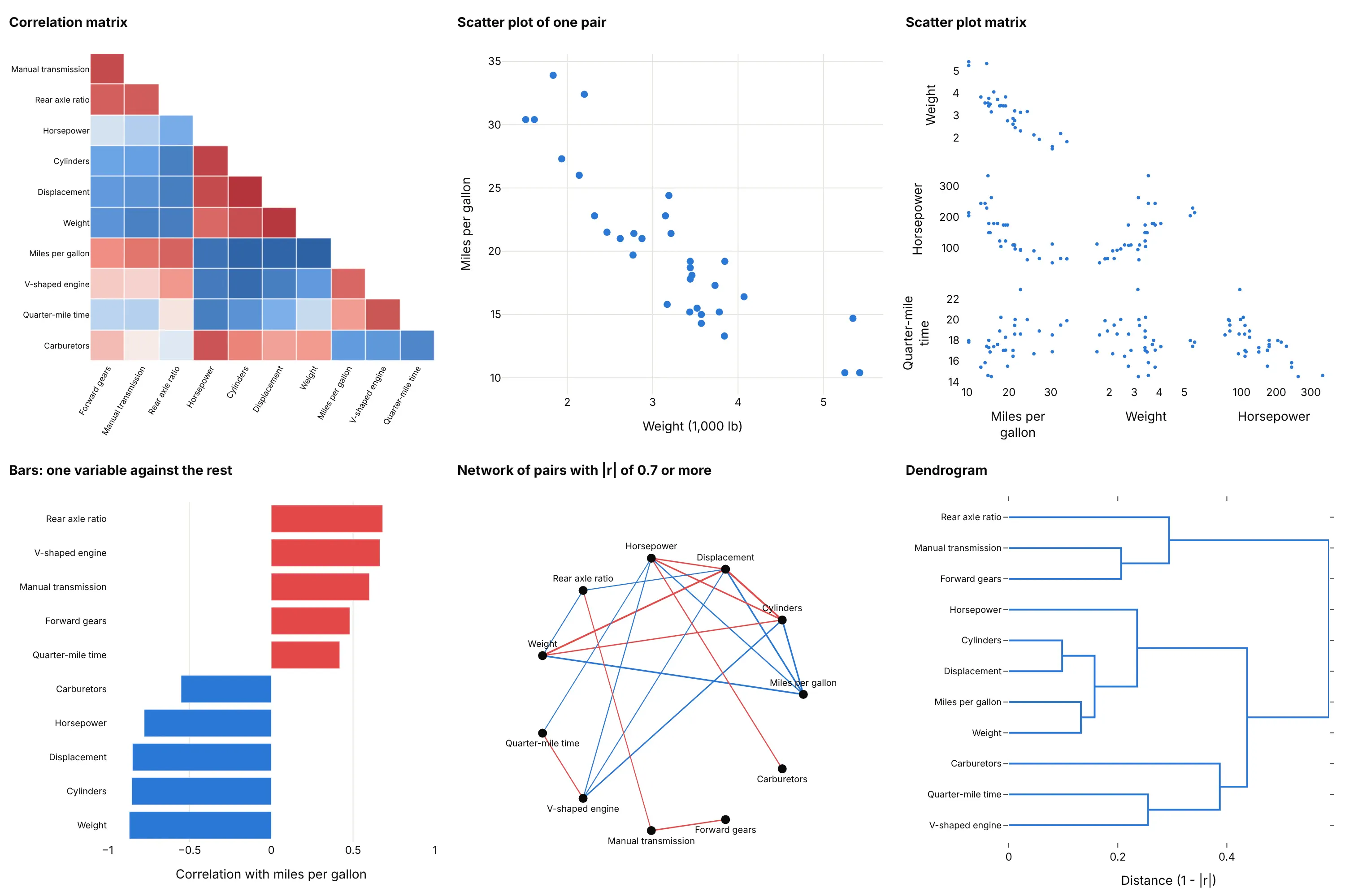
- Scatter plot (better for one pair). It shows the shape of the relationship, which a coefficient can't, such as a curve or an outlier (example 5 below). Use it to check any pair that matters, like weight against miles per gallon at r = -0.87.
- Scatter plot matrix (better for up to about six variables). Every pair gets its own scatter plot, so shapes and outliers are visible, but 4 variables already need 6 plots and the 11 here would need 55.
- Bar chart of correlations with one variable (better when one outcome matters). If you only care about miles per gallon, sorted bars show that weight (-0.87), cylinders (-0.85) and displacement (-0.85) lead, and they are easier to compare than colors. It drops all the other pairs.
- Network graph (different). Variables become nodes and strong pairs become edges, here the 19 of 55 pairs with a correlation of 0.7 or more in absolute value. It suits large sets with clear groups and hides the weak links.
- Dendrogram (works too, for the grouping). The tree shows which variables merge first, cylinders and displacement at a distance of 0.10, but not the value of any single pair. A clustered correlation matrix plot gives you both.
Our heatmap guide shows another clustered correlation matrix, of 18 asset-class exchange-traded funds, and the general design of heatmaps.
How to make a correlation matrix plot
With AI
ChatGPT, Claude Code, GitHub Copilot, Cursor and other AI tools are excellent at writing Plotly code. Name Plotly in the prompt, and say how to order the variables, which coefficient to use and how to color the cells:
Make a plotly correlation matrix plot from data.csv (one row per observation, numeric columns are the variables).- Compute df.corr(method="spearman") if any column is skewed, otherwise Pearson; drop rows with missingvalues first and print how many were left.- Order rows and columns by average-linkage clustering on 1 - |r| (scipy, optimal_leaf_ordering).- Show only the lower triangle without the diagonal, with the coefficient printed in each cell to 2 decimals.- Diverging blue-white-red colorscale with zmin=-1, zmax=1 and zmid=0, a colorbar titled "Correlation".- Inter font, white background, tilted x labels, and a title that states the main finding.
With Plotly Studio
Plotly Studio is a product for creating data visualizations and Dash apps and for analyzing data with AI, available as a desktop app or embedded in Dash apps. Ask for a correlation matrix the same way:
Show a correlation matrix plot of the numeric columns in this file, lower triangle only, ordered by hierarchical clustering, with the coefficient in each cell and a blue-white-red scale fixed at -1 to 1. Add a dropdown to switch between Pearson and Spearman and a slider for the date range.
Make a correlation matrix plot in Python or JavaScript
This is the code AI tools write under the hood. In Python, df.corr() calculates the matrix, scipy orders it, and px.imshow draws it. This example uses the six tech stocks in px.data.stocks:
import numpy as npimport plotly.express as pxfrom scipy.cluster.hierarchy import leaves_list, linkage, optimal_leaf_orderingfrom scipy.spatial.distance import squareformreturns = px.data.stocks(indexed=True).pct_change().dropna() # six tech stocks, weeklycorr = returns.corr() # method="spearman" for rank correlationdist = squareform(1 - corr.to_numpy(), checks=False) # similar stocks are close togetherorder = leaves_list(optimal_leaf_ordering(linkage(dist, "average"), dist))corr = corr.iloc[order, order]lower = corr.where(np.tril(np.ones(corr.shape, dtype=bool), k=-1)) # keep each pair oncefig = px.imshow(lower.iloc[1:, :-1], text_auto=".2f", zmin=-1, zmax=1,color_continuous_scale="RdBu_r", color_continuous_midpoint=0)fig.show()
For the full square without clustering, px.imshow(df.corr(), zmin=-1, zmax=1, color_continuous_scale="RdBu_r") is enough. To show significance, mask the cells whose adjusted p-value is above 0.05 with corr.where(p < 0.05), as in example 3.
In JavaScript, plotly.js takes the matrix as z, with null for the cells to leave empty. This example draws the lower triangle of four car measurements:
<div id="chart"></div><script src="https://cdn.plot.ly/plotly-4.1.1.min.js"></script><script>// Correlations of four measurements of 32 cars (Motor Trend, 1973-74), lower triangle onlyPlotly.newPlot("chart", [{type: "heatmap",x: ["Miles per gallon", "Weight", "Horsepower"],y: ["Weight", "Horsepower", "Quarter-mile time"],z: [[-0.87, null, null], [-0.78, 0.66, null], [0.42, -0.17, -0.71]],zmin: -1, zmax: 1, zmid: 0,colorscale: "RdBu",texttemplate: "%{z:.2f}", hoverongaps: false, xgap: 2, ygap: 2}], {width: 640, height: 420, margin: {l: 130}, yaxis: {autorange: "reversed"}});</script>
The two libraries name the red-blue scale in opposite directions, so RdBu_r in Python and RdBu in plotly.js both put blue at -1 and red at 1.
Share it
Every Plotly chart has a Share chart button (the cloud icon in its toolbar) that uploads it to Plotly Cloud and gives you a link. Only you can see it until you change its visibility.
For a live app, put the chart in a Dash app and publish it with the Plotly Cloud command-line interface (CLI). Coding agents can run these commands for you:
pip install "dash[cloud]"plotly user loginplotly app publish
If your data has to stay in your own cloud or data center, publish to Dash Enterprise instead.
Dos and don'ts
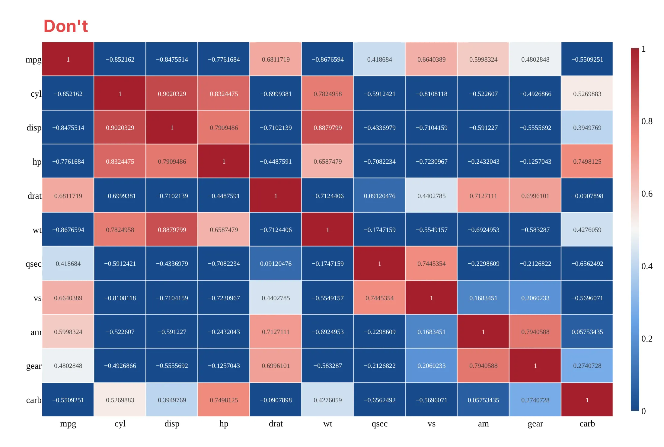
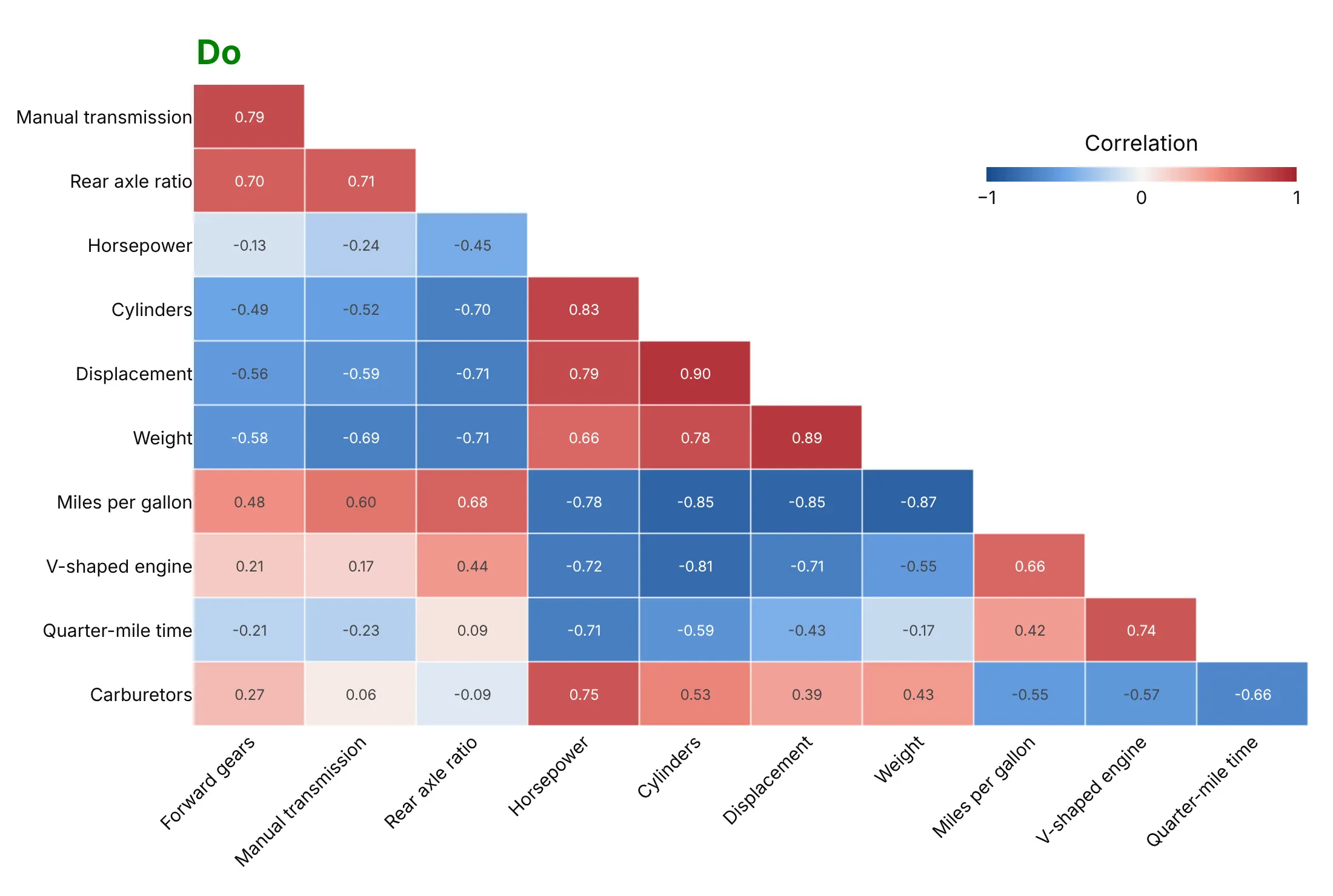
Plotly keeps the variables in the order of your data and stretches the color scale over whatever range you give it, so the defaults need a few changes for a correlation matrix. Here is the same car matrix both ways, with the same blue-white-red colors.
Don't leave the variables in the order of the file with their raw column names, draw a color scale from 0 to 1 so that every negative correlation turns the same dark blue as a correlation of 0, repeat each pair in both halves of the square with a diagonal of 1s, print values with seven digits that overflow the cells, or use a serif font:
Do order the variables by clustering and name them in words, fix the scale from -1 to 1 with white at 0, draw only the lower triangle, and print the coefficient to two decimals:
Checklist
Do
- Fix the color scale at -1 to 1 with the midpoint at 0, so colors mean the same in every matrix you draw and can be compared (example 1 below).
- Order the variables by hierarchical clustering, on 1 - |r| when the sign doesn't matter for grouping.
- Draw one triangle without the diagonal and print the coefficient when there are fewer than about 400 cells (20 by 20), with hover only above that.
- Say which coefficient, how many observations, and what you did with missing values and outliers.
- Look at the scatter plot of any pair you are going to talk about, and use Spearman when the variables are skewed (example 2).
- Mark which cells are significant when the sample is small (example 3).
Don't
- Read a correlation as cause and effect. Two variables can move together because a third drives both, as in the shared daily cycle of example 4.
- Compare matrices that cover different periods or sample sizes without saying so, because a short window gives noisy coefficients.
- Drop the sign by plotting |r| unless you say so, because it hides the pairs that move in opposite directions.
- Treat a coefficient near 0 as "unrelated". Pearson only measures straight-line relationships, and a perfect curve can have r = 0.
More correlation matrix plot examples
Six more correlation matrix plots built from real public data, each with its source, a tip and a prompt to rebuild it.
1. Correlations spike in a crisis
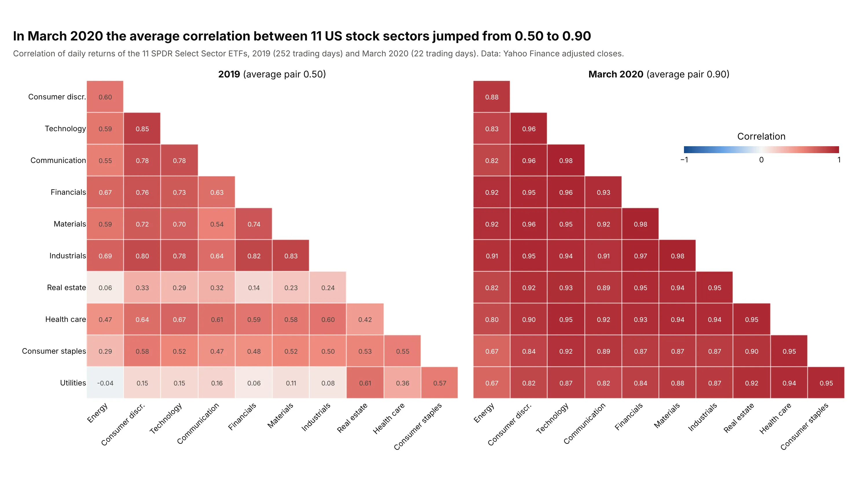
Diversification relies on assets that don't move together, and in March 2020 the average correlation between 11 US stock sectors rose from 0.50 in 2019 to 0.90, with no pair below 0.67 (the lowest, energy and utilities, had been at -0.04). March 2020 covers only 22 trading days, so each coefficient is noisier than the 2019 ones, but every pair is above the 0.42 that 22 days need to be significant at 0.05. Data: Yahoo Finance adjusted closes of the 11 Select Sector SPDR exchange-traded funds (ETFs), which each hold the stocks of one sector of the S&P 500.
Tip: draw both periods in the same order and on the same fixed scale, so the change shows up as color alone.
Get the data from Yahoo Finance: daily adjusted closes of the 11 Select Sector SPDR ETFs (XLK, XLC, XLY, XLF, XLI, XLB, XLE,XLV, XLP, XLU, XLRE) from 2018-06-19 to 2025-12-31 (columns: date plus one column per ticker).Compute daily returns with pct_change. Build two plotly lower-triangle correlation heatmaps side by side with one -1 to 1blue-white-red scale (zmid=0): all of 2019, and March 2020. Order both by clustering the March 2020 matrix, label each cell,and put the mean of the 55 pairwise correlations in each subplot title.
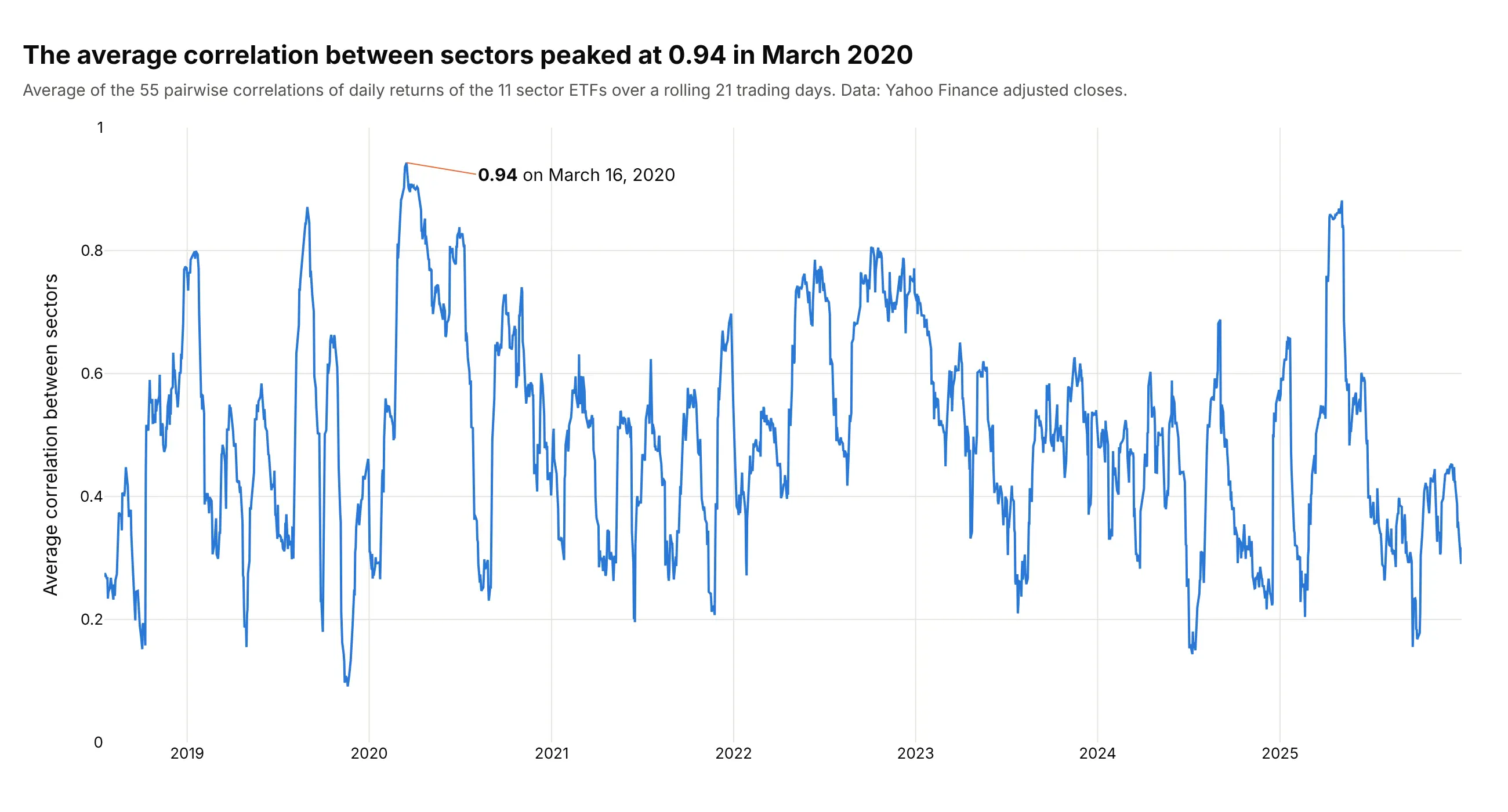
Another way to see it: a line of the average pairwise correlation over a rolling 21 trading days shows when it happened and how often it has happened since, peaking at 0.94 on March 16, 2020 and at 0.88 on May 5, 2025.
2. Pearson against Spearman
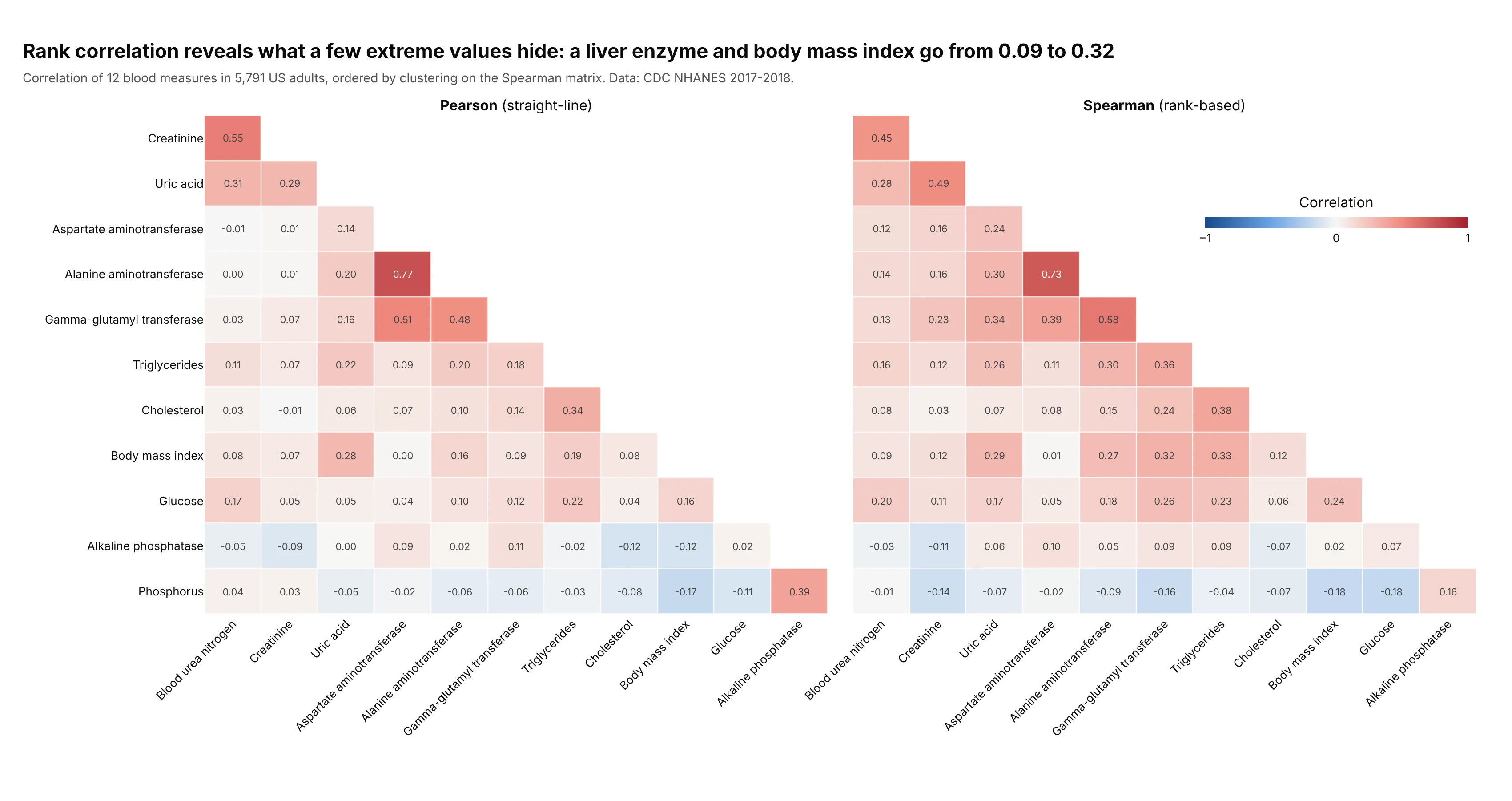
Many blood tests are skewed, with a few very high values. Gamma-glutamyl transferase (GGT), a liver enzyme, has a median of 19 units per liter (U/L) and a maximum of 1,192 U/L, which pulls the Pearson coefficient with body mass index (BMI) down to 0.09, while the rank-based Spearman coefficient is 0.32. Uric acid and creatinine go from 0.29 to 0.49 the same way. Data: CDC NHANES 2017-2018, 5,791 adults with all 12 measures.
Tip: draw both matrices in the same row order and on the same scale, and read the cells that differ most, which are the ones that outliers or curves are affecting.
Get the data from the CDC National Health and Nutrition Examination Survey 2017-2018, the Standard Biochemistry ProfileBIOPRO_J.xpt and Body Measures BMX_J.xpt (columns: LBXSATSI, LBXSASSI, LBXSGTSI, LBXSTR, LBXSGL, LBXSUA, LBXSBU, LBXSCR,LBXSAPSI, LBXSPH, LBXSCH and BMXBMI, joined on SEQN).Keep adults with all 12 values. Build two plotly lower-triangle correlation heatmaps side by side, Pearson and Spearman(df.corr(method="spearman")), in the order of clustering the Spearman matrix, with one -1 to 1 scale and 2-decimal labels.
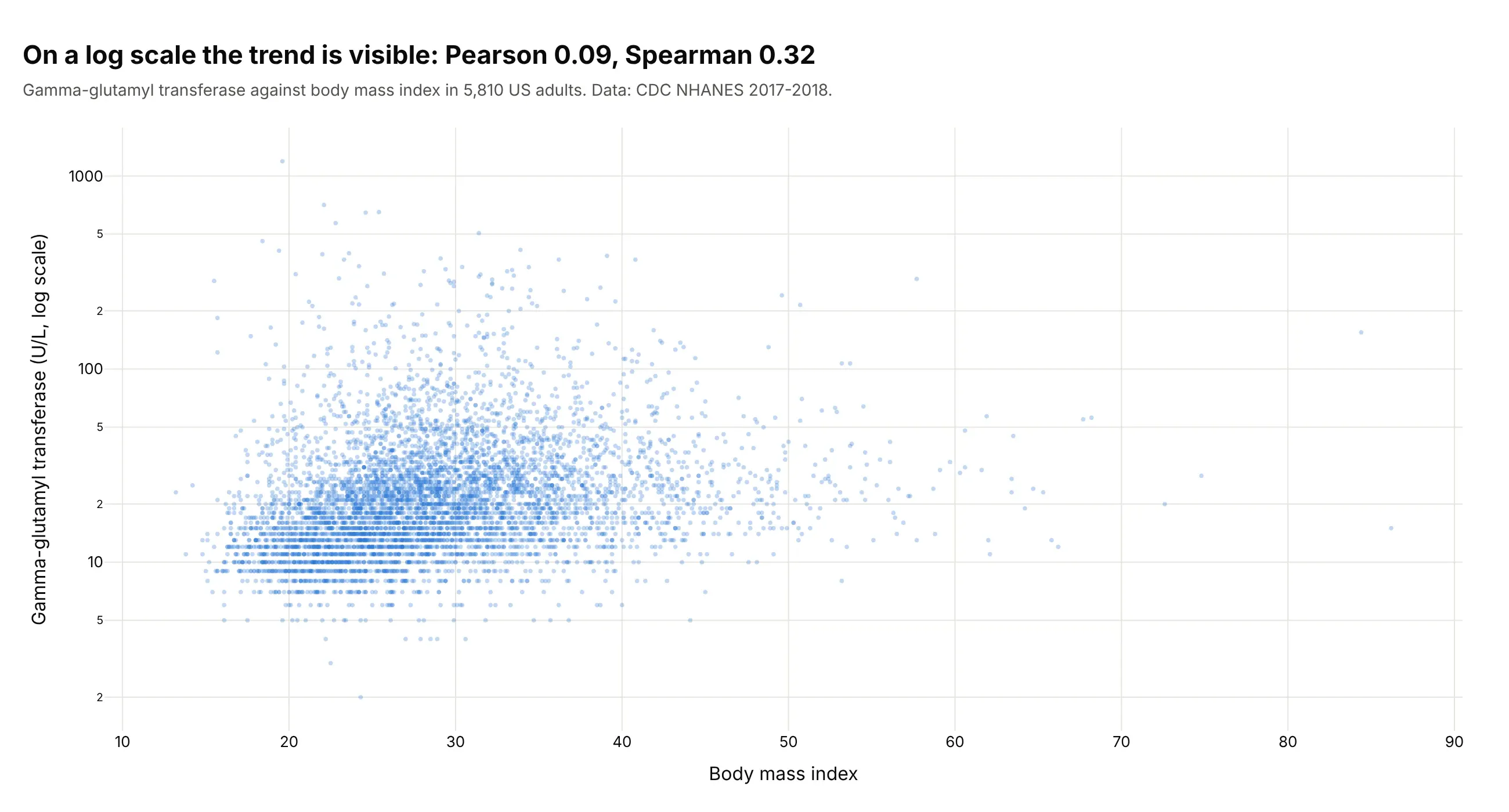
Another way to see it: the scatter plot of GGT against BMI on a log axis shows the upward trend that a few extreme values hide from Pearson.
3. Which correlations are significant
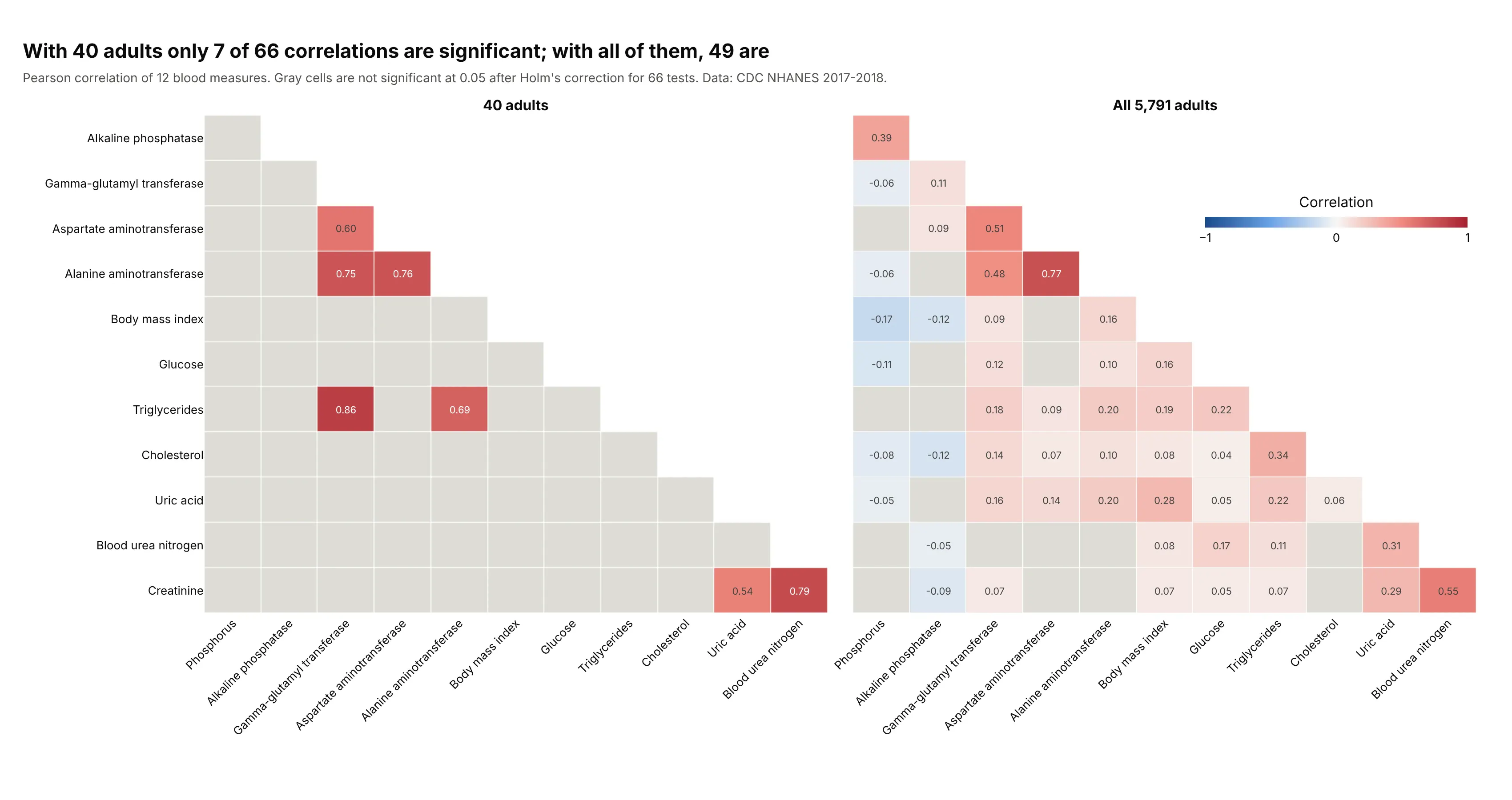
In a random sample of 40 adults, 7 of the 66 pairs are significant at 0.05 after Holm's correction, and in all 5,791 adults 49 are. Significance is not accuracy, though, because the sample of 40 shows GGT and triglycerides at 0.86, which is significant, when the full data give 0.18. One adult with a GGT of 256 U/L and triglycerides of 846 milligrams per deciliter (mg/dL) creates it, and without that person the sample's coefficient is 0.01. Another sample of 40 would give a different set, from 1 to 7 significant pairs across five different seeds. Data: CDC NHANES 2017-2018.
Tip: gray out the cells that don't pass, instead of deleting them, so readers can see that they were tested.
Get the data from the CDC National Health and Nutrition Examination Survey 2017-2018, the Standard Biochemistry ProfileBIOPRO_J.xpt and Body Measures BMX_J.xpt (columns: LBXSATSI, LBXSASSI, LBXSGTSI, LBXSTR, LBXSGL, LBXSUA, LBXSBU, LBXSCR,LBXSAPSI, LBXSPH, LBXSCH and BMXBMI, joined on SEQN).Keep adults with all 12 values and take df.sample(40, random_state=1). For the sample and for everyone, compute the Pearsonmatrix, the p-values from t = r * sqrt((n - 2) / (1 - r**2)), and Holm-adjusted p-values over the 66 pairs(statsmodels multipletests). Build two plotly lower-triangle heatmaps side by side with a -1 to 1 scale, a flat gray cellwhere the adjusted p-value is 0.05 or more, and a title with the number of significant pairs in each.
4. A shared cycle inflates correlations
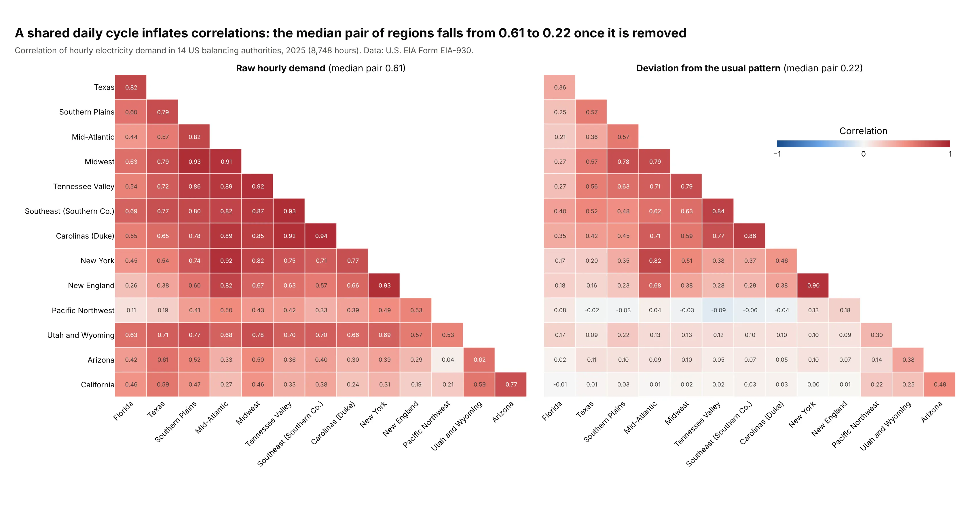
Raw hourly demand in the 14 grid operators has a median pair correlation of 0.61, with California and the Mid-Atlantic at 0.27, only because everyone uses more power in the evening and in summer. After subtracting each one's usual value for that month, day type and hour, the median falls to 0.22 and California and the Mid-Atlantic to 0.01, and regional groups appear. Data: U.S. EIA, Form EIA-930, 8,748 hours of 2025.
Tip: when series share a strong trend or season, remove it (or use changes instead of levels) before correlating, or the matrix will show the season.
Get the data from the U.S. Energy Information Administration Form EIA-930 Hourly Electric Grid Monitor, the 2025 six-monthBALANCE files (https://www.eia.gov/electricity/gridmonitor/sixMonthFiles/), column "Demand (MW) (Adjusted)" for the balancingauthorities CISO, ERCO, ISNE, MISO, NYIS, PJM, SWPP, SOCO, TVA, DUK, FPL, BPAT, PACE and AZPS, keyed by UTC time.Pivot to one column per authority, replace hours under half or over double the weekly median with gaps and interpolate them.Compute a second table of deviations from the mean for the same local month, weekday or weekend, and hour. Build two plotlylower-triangle correlation heatmaps side by side (raw and deviations), same order from clustering the deviations, one -1 to 1scale, and the median pair in each title.
5. Outliers and curves
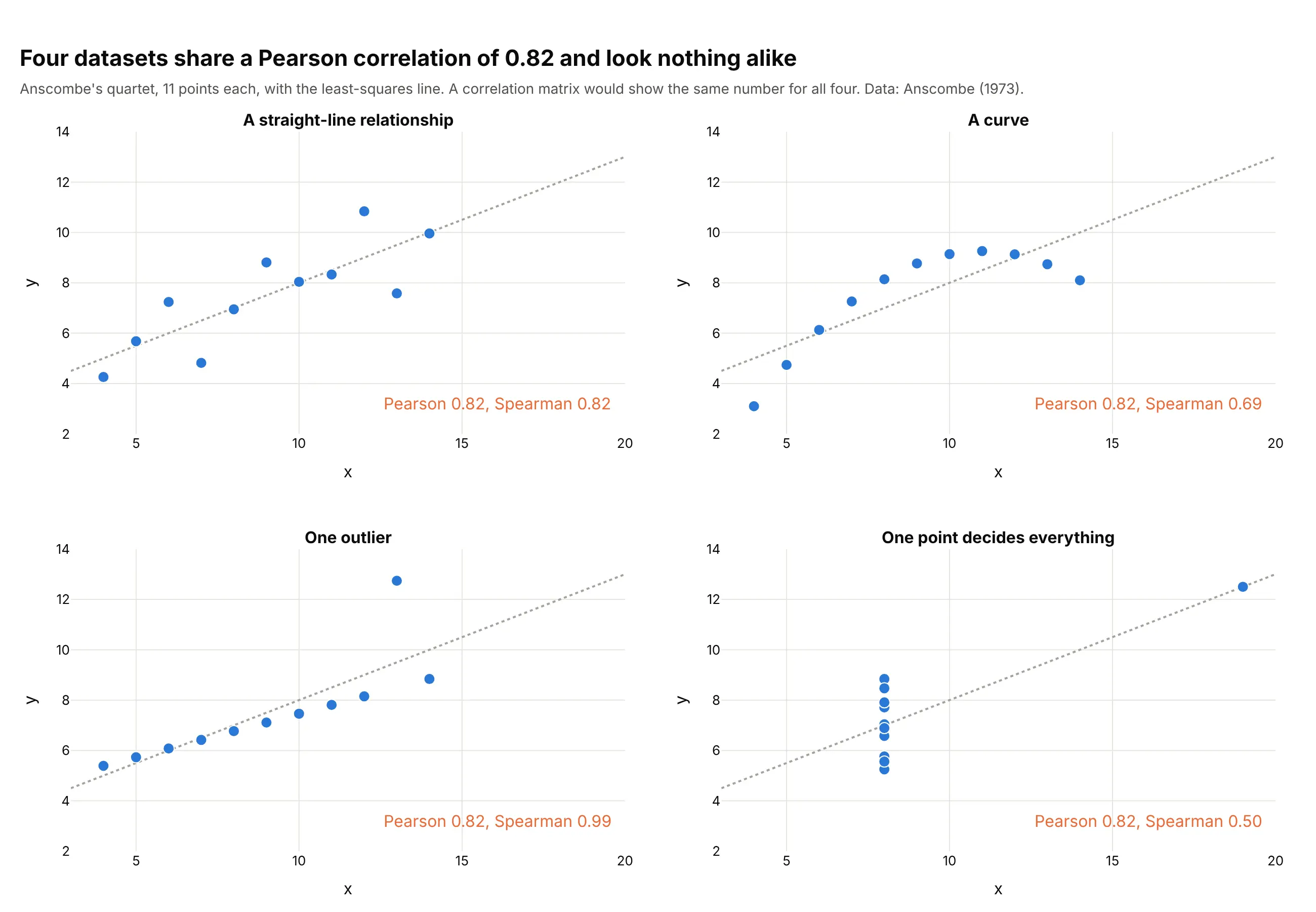
Anscombe's four small datasets all have a Pearson correlation of 0.82 (0.816 to 0.817) and the same fitted line, yet one is a curve, one has an outlier and in one a single point at the far right creates the whole relationship. The Spearman coefficients (0.82, 0.69, 0.99 and 0.50) separate them better, though still not completely. A correlation matrix would show the same cell four times. Data: Anscombe (1973), 11 points per set.
Tip: put the scatter plot of any pair you care about next to the matrix, with both coefficients printed on it.
Get the data from Anscombe's quartet (Anscombe 1973, The American Statistician 27, 17-21), as in the R datasets table anscombe(columns: x1 to x4 and y1 to y4, 11 rows).Build a 2 x 2 plotly figure of scatter plots (x1 against y1 and so on) with the least-squares line dotted gray, and in eachpanel the Pearson and Spearman coefficients (scipy.stats.spearmanr) in orange text, and a title stating that all four share aPearson correlation of 0.82.
6. A wide matrix of 30 measurements
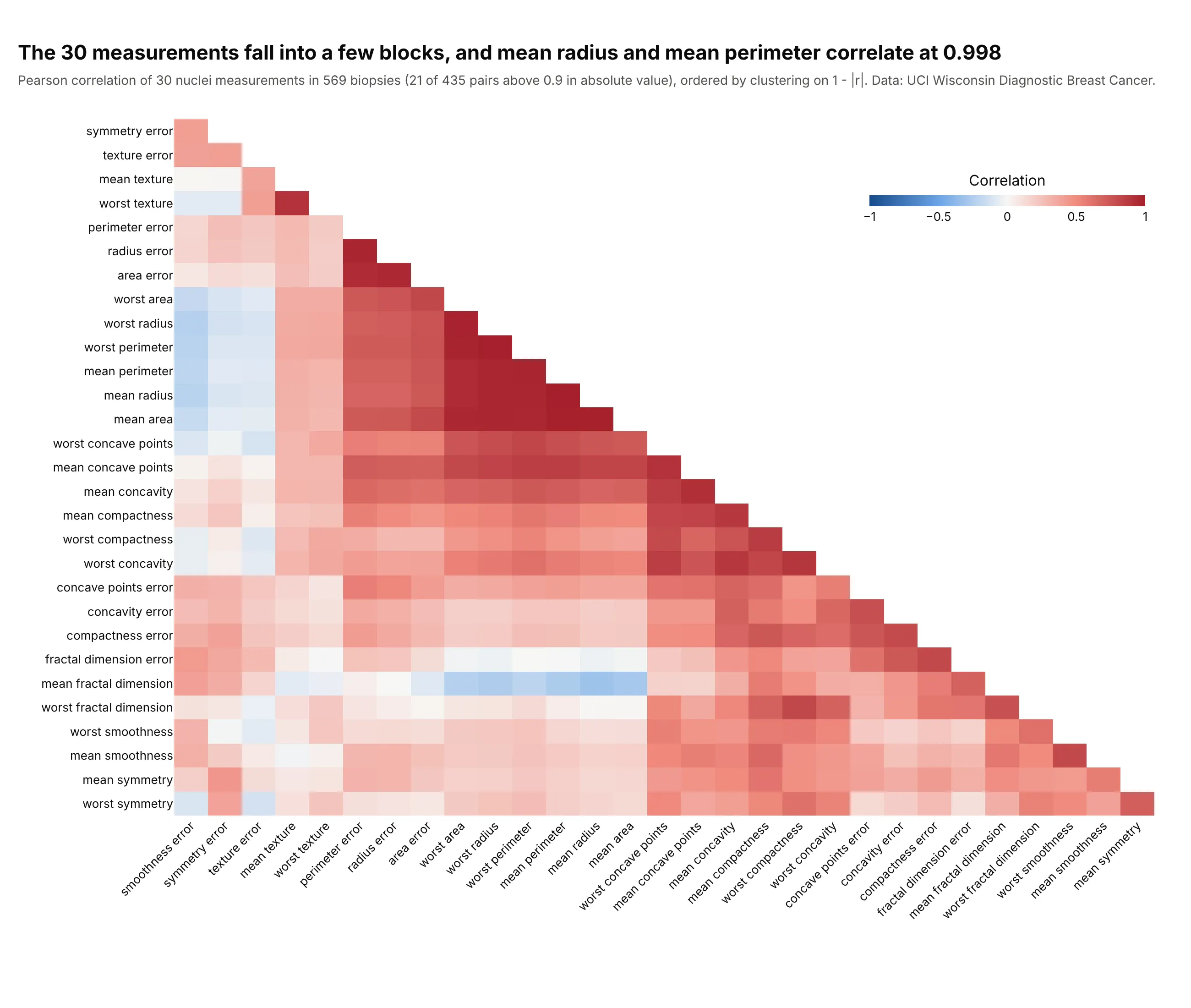
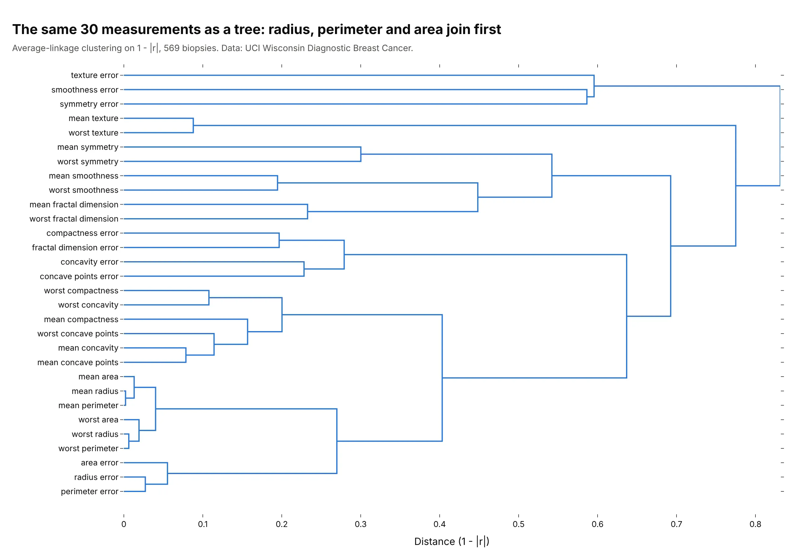
Thirty measurements of cell nuclei in 569 breast biopsies (the mean, standard error and worst value of each of 10 features) give 435 pairs, 21 of them above 0.9 in absolute value. The largest block holds radius, perimeter and area, because perimeter and area are nearly determined by radius (mean radius and mean perimeter correlate at 0.998), so a model fitted on all 30 would be fitting some of the same information several times. With this many cells the numbers are left to the hover text. Data: Breast Cancer Wisconsin (Diagnostic), UCI Machine Learning Repository, as bundled with scikit-learn.
Tip: above about 400 cells, drop the printed numbers and the cell gaps and let the clustering and the colors carry the picture.
Get the data from the Breast Cancer Wisconsin (Diagnostic) dataset of the UCI Machine Learning Repository, or sklearn.datasets.load_breast_cancer(columns: the 30 measurements such as mean radius, mean texture and worst concave points; ignore the diagnosis).Build a plotly lower-triangle correlation heatmap of the 30 measurements ordered by average-linkage clustering on 1 - |r|, noprinted values, no gaps between cells, a -1 to 1 blue-white-red scale, and hover showing both names and the coefficient. Put thecount of pairs above 0.9 in the subtitle.
Another way to see it: a dendrogram of the same 30 measurements shows how the groups merge, with the mean radius, perimeter and area joining at distances below 0.02.
FAQ
Options to customize
A correlation matrix plot in Plotly is a heatmap with a fixed color scale and a matrix that you prepare, so these are the options that matter most. The full lists are in the heatmap trace reference and the imshow documentation.
- zmin=-1, zmax=1, zmid=0 (px.imshow: zmin, zmax, color_continuous_midpoint): fix the color scale so white is 0 and colors are comparable between matrices.
- colorscale (px.imshow: color_continuous_scale): a diverging scale such as RdBu_r in Python or a list of colors; blue for negative and red for positive is the usual choice.
- texttemplate="%{z:.2f}" (px.imshow: text_auto=".2f"): print the coefficient in each cell, with textfont.size to fit.
- xgap and ygap: thin white lines between cells, useful up to about 30 variables.
- A masked z: set the upper triangle (and the diagonal) to NaN or None to draw only the lower triangle, and drop the empty first row and last column.
- hoverongaps=False and hovertemplate: no hover on empty cells, and a hover that names both variables, the coefficient and, with customdata, the p-value or the sample size.
- yaxis.autorange="reversed": puts the first variable at the top so the matrix reads like a table.
- xaxis.tickangle: tilt long variable names at -45 degrees.
- colorbar.orientation="h", x, y, len: put the colorbar in the empty upper triangle.
- A second go.Heatmap with a single flat color: gray out cells that are not significant, as in example 3.
- make_subplots with shared_yaxes=True: two matrices side by side on one scale, for two periods or two methods.
- plotly.figure_factory.create_dendrogram and go.Splom: the dendrogram and the scatter plot matrix that go with a correlation matrix.