Chris Parmer

November 4, 2026

Dendrograms - A Complete Guide

TL;DR

A dendrogram is the tree that hierarchical clustering produces: every item is a leaf, and each pair of branches joins at the height (the distance) where the two groups were merged, so low joins mean similar items and high joins mean different ones.
Dendrograms are also known as tree diagrams, cluster trees, phylogenetic trees (in biology) and, drawn on the edges of a heatmap, clustergrams, and are similar to treemaps and icicle charts, which also draw a hierarchy, and minimum spanning tree network graphs.
You get clusters by cutting the tree at a height: every branch that crosses the cut is one cluster. Where you cut, and which linkage method you use (single, complete, average or Ward), changes the clusters, so say both on the chart.
They are the standard chart for gene expression clustering and phylogenetics, and they also group stocks by correlation, countries by energy mix and drugs by safety profile.
You can make a dendrogram with Plotly in Python with plotly.figure_factory.create_dendrogram, which runs SciPy's clustering and draws the tree, or a clustered heatmap with Dash Bio's Clustergram.

What is a dendrogram?

Dendrograms look like this:

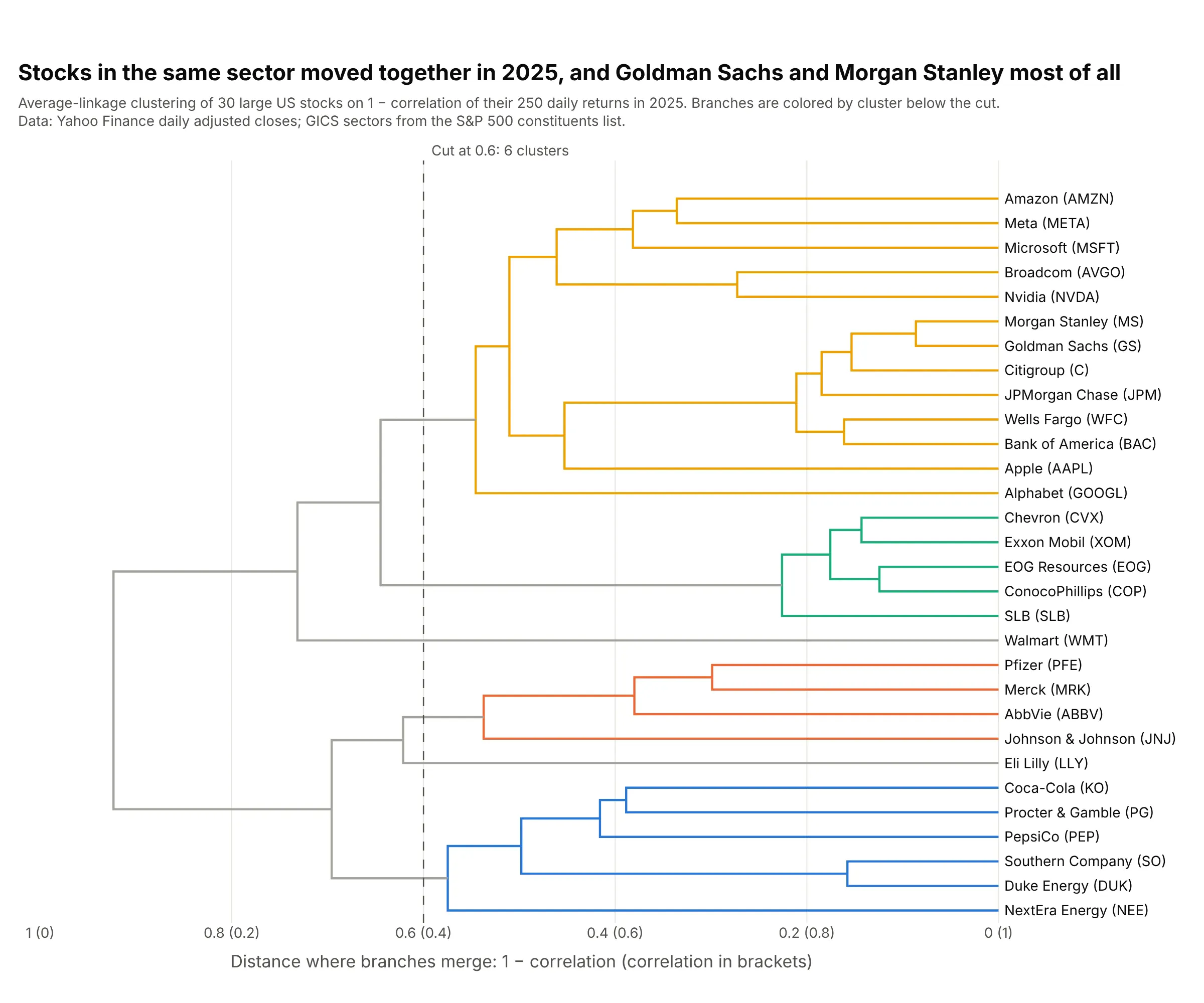
Horizontal dendrogram of 30 large US stocks clustered on 1 minus the correlation of their 2025 daily returns: Goldman Sachs and Morgan Stanley merge first near 0.09, the five energy stocks join by 0.23, utilities and consumer staples form one blue cluster, four drug makers an orange one, energy a green one, and banks with big tech a yellow one, with a dashed cut at 0.6 giving 6 clusters including Eli Lilly and Walmart on their own

Data: Yahoo Finance daily adjusted closes for 2025; GICS sectors from the S&P 500 constituents list.

How do you read a dendrogram? In the example above, notice these things:

Each leaf on the right is one stock, and the distance between two stocks is 1 minus the correlation of their 250 daily returns in 2025, so 0 means they moved in lockstep and 1 means they were unrelated.
Follow two leaves left until their branches meet: the height of that join is how far apart they are. Goldman Sachs and Morgan Stanley join first, at 0.086 (a correlation of 0.914), and all five energy stocks have joined by 0.226.
Groups merge with groups the same way. With average linkage, used here, a join's height is the average distance between every stock on one side and every stock on the other, so the last join at 0.923 says the two halves of the tree are almost uncorrelated.
The dashed line is a cut at 0.6. Every branch that crosses it is a cluster, which gives 6: utilities and staples, four drug makers, energy, banks with big tech, and Eli Lilly and Walmart on their own.
Only the joins carry information. You can flip any branch around its join without changing the tree, so two stocks drawn next to each other aren't necessarily close; read the height where they meet.

It's often used for charts like these:

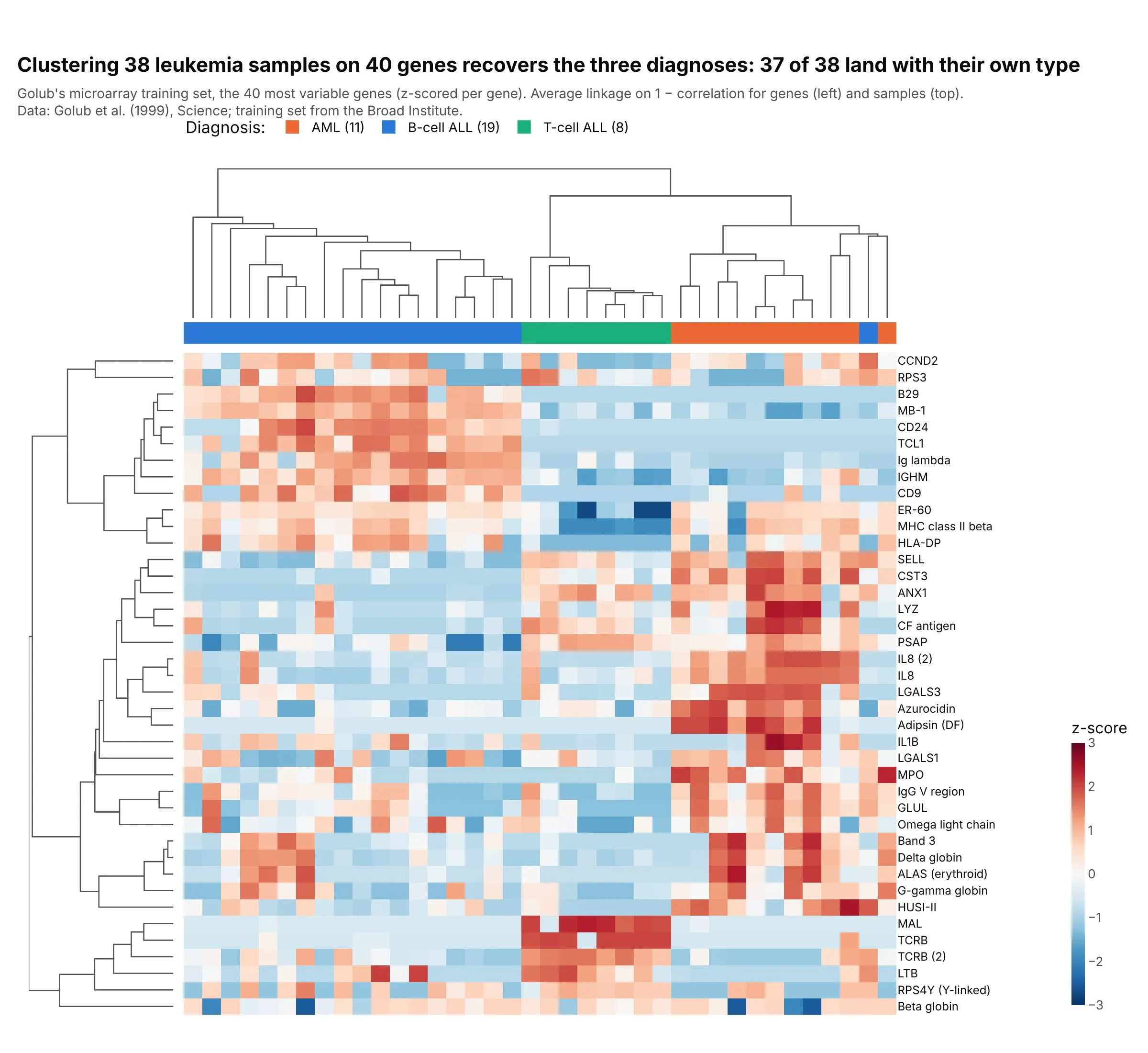
Clustered heatmap of 40 genes by 38 leukemia samples with dendrograms on the rows and columns and a strip of diagnosis colors: the sample tree separates 18 B-cell ALL samples in blue, 8 T-cell ALL in green and 11 AML in orange plus one B-ALL sample, with blocks of red for T-cell genes like TCRB and MAL and myeloid genes like LYZ and MPO

Gene expression (clustered heatmaps). Clustering Golub's 38 leukemia microarrays on their 40 most variable genes, without the diagnoses, puts 37 of 38 samples with their own type: B-cell ALL, T-cell ALL or AML. Data: Golub et al. (1999), training set from the Broad Institute.

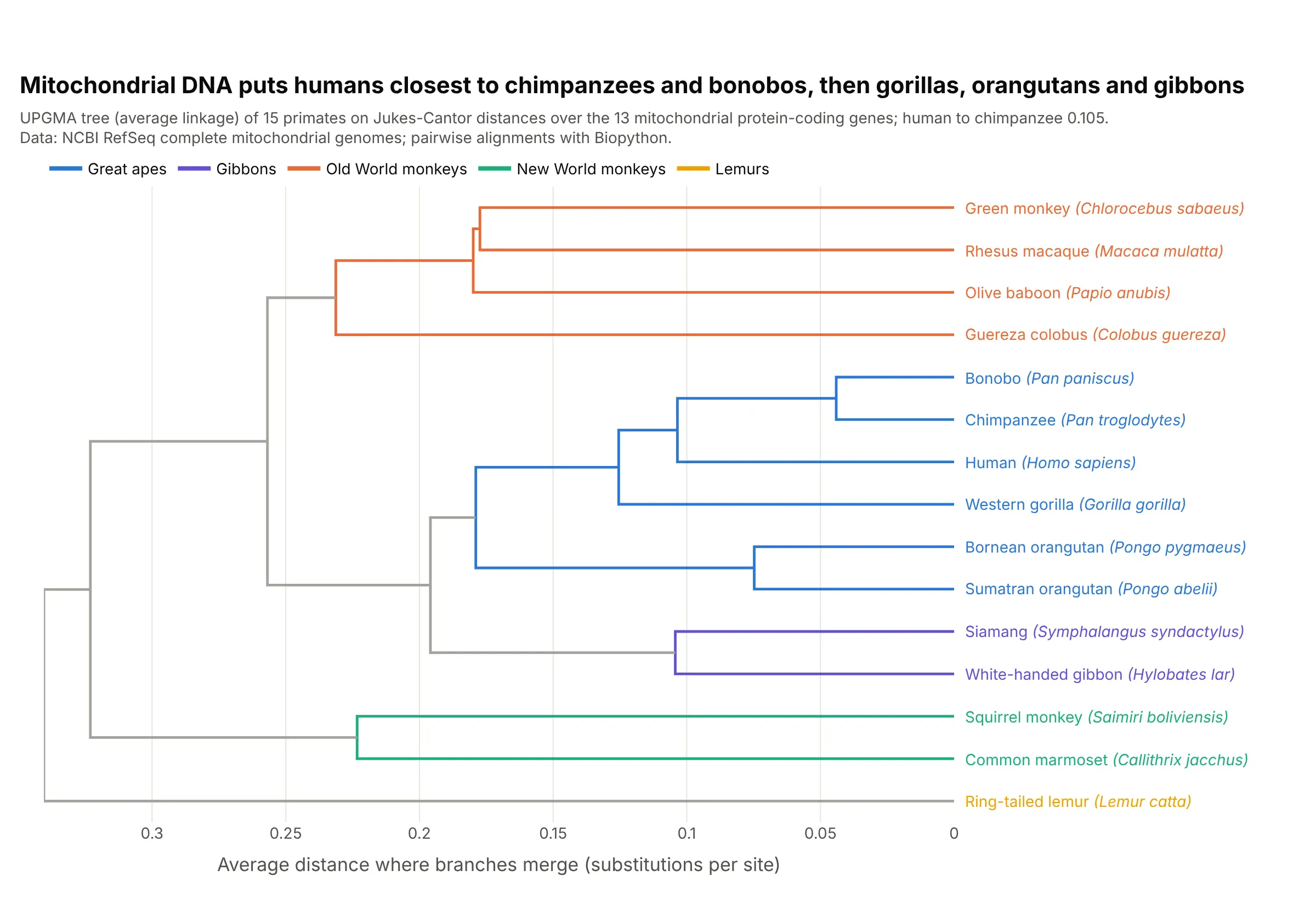
Phylogenetic tree of 15 primates from 13 mitochondrial genes: chimpanzee and bonobo join first at 0.044, human joins them at 0.10, then gorilla, the two orangutans and the gibbons, with Old World monkeys, New World monkeys and the ring-tailed lemur joining further left

Phylogenetic trees. On the 13 protein-coding genes of the mitochondrial genome, humans are 0.105 substitutions per site from chimpanzees and closer to them than to gorillas, orangutans or gibbons. The tree uses UPGMA, the textbook distance method, which is average linkage. Data: NCBI RefSeq complete mitochondrial genomes.

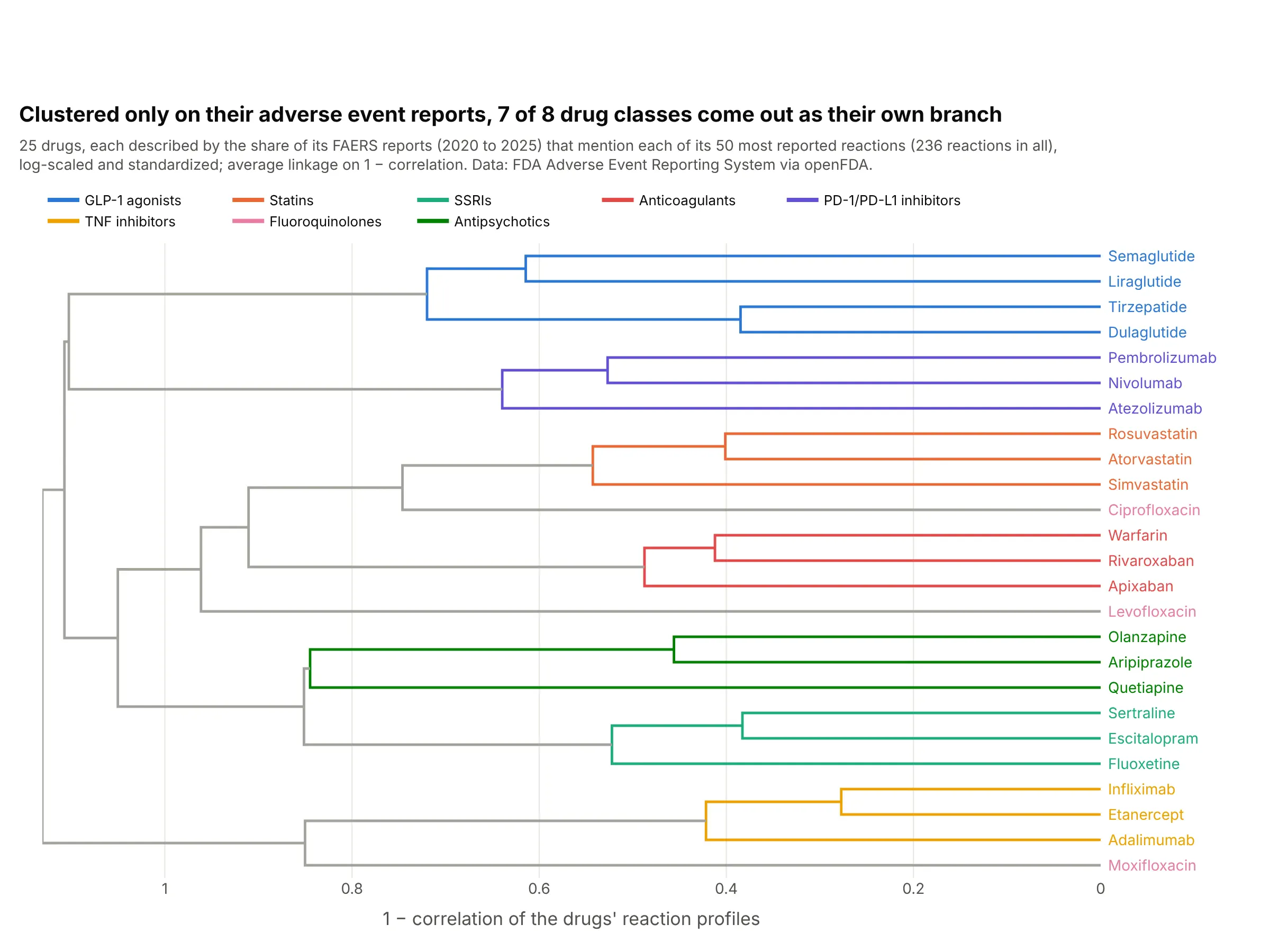
Dendrogram of 25 drugs clustered on their FDA adverse event report profiles, with GLP-1 agonists, PD-1 inhibitors, statins, anticoagulants, antipsychotics, SSRIs and TNF inhibitors each forming their own colored branch, and the three fluoroquinolones scattered

Drug safety profiles. Clustered only on which reactions appear in their 2020 to 2025 FDA adverse event reports, 7 of 8 drug classes come out as their own branch; the three fluoroquinolones land in three different places. Data: FDA Adverse Event Reporting System via openFDA.

How to cut a dendrogram into clusters

A dendrogram holds every possible clustering of the data at once, from one cluster per item at the bottom to a single cluster at the top. Cutting it at a height picks one: each branch that crosses the cut becomes a cluster, as the dashed lines in the examples above and below show.

There are two common ways to choose the cut. Pick a height that means something in your units (a correlation of 0.4 between stocks, a distance of 0.6), or pick the number of clusters you need and cut wherever that many branches cross. Long vertical stretches with no joins are where a cut is most stable, because moving it a little doesn't change the clusters. In Python, SciPy's fcluster gives each item its cluster number either way, and create_dendrogram's color_threshold colors the branches below the same height:

from scipy.cluster.hierarchy import fcluster, linkage

Z = linkage(distances, "average")                  # distances: condensed matrix from pdist or squareform
by_height = fcluster(Z, t=0.6, criterion="distance")  # cut at 0.6
by_count = fcluster(Z, t=4, criterion="maxclust")      # or ask for 4 clusters

Linkage methods: single, complete, average and Ward

Once two items are merged, the algorithm needs a rule for the distance from that group to everything else. That rule is the linkage method, and it changes the tree more than most people expect. Here is the NCI60 dataset from An Introduction to Statistical Learning, 64 cancer cell lines and 6,830 genes, clustered four ways and each tree cut into four clusters:

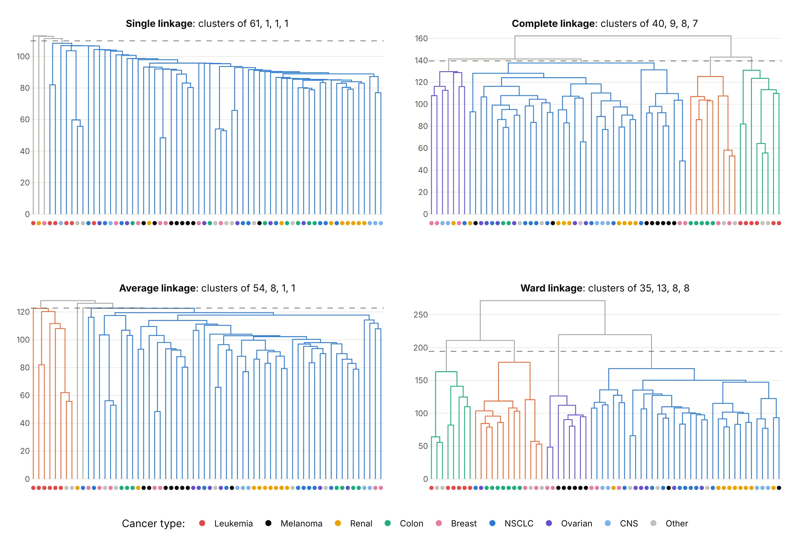
Four dendrograms of the same 64 NCI60 cancer cell lines: single linkage chains into clusters of 61, 1, 1 and 1; complete linkage gives 40, 9, 8 and 7; average linkage 54, 8, 1 and 1; Ward linkage 35, 13, 8 and 8, with the six leukemia lines in one cluster in every method but single

Data: NCI60 from the ISLR package (Ross et al. 2000), genes scaled to standard deviation 1, Euclidean distance.

Single linkage uses the closest pair between two groups. It finds long chains, so one item at a time joins a growing blob: 61, 1, 1 and 1 here.
Complete linkage uses the farthest pair, which gives compact clusters of similar size (40, 9, 8 and 7). It's the default in create_dendrogram and Dash Bio.
Average linkage uses the average distance over all pairs. It's what UPGMA trees in phylogenetics use, and it works with any distance, including 1 − correlation.
Ward linkage merges the pair that adds the least within-cluster variance (Ward 1963), which gives the most balanced clusters (35, 13, 8 and 8). It assumes Euclidean distances.

Six of the 64 lines are leukemias, and complete, average and Ward linkage all keep them together. When a grouping survives every method like that, you can trust it more than one that only one method finds.

A short history

The name comes from the Greek for tree and drawing, and tree diagrams of related species go back at least to the evolutionary tree in Darwin's On the Origin of Species (1859). Dendrograms as a statistical chart came with numerical taxonomy in the 1950s, when Sneath (1957) described using computers for taxonomy and Sokal and Michener published UPGMA, the average-linkage method the primate tree above uses. Ward (1963) added the minimum-variance method. Eisen et al. (1998) showed gene clusters and the expression values behind them in one display, the kind of clustered heatmap shown above, and Wilkinson and Friendly (2009) wrote the history of the cluster heat map. In finance, Mantegna (1999) clustered stocks on the correlation of their returns, as the first example on this page does. We didn't redraw an original figure because none of these papers' data is public in a form we could check; the Golub and primate examples show the same kinds of chart on public data.

Alternatives to a dendrogram

Here's the same 30-stock data drawn five ways. Some are better for the question, some worse, some just different:

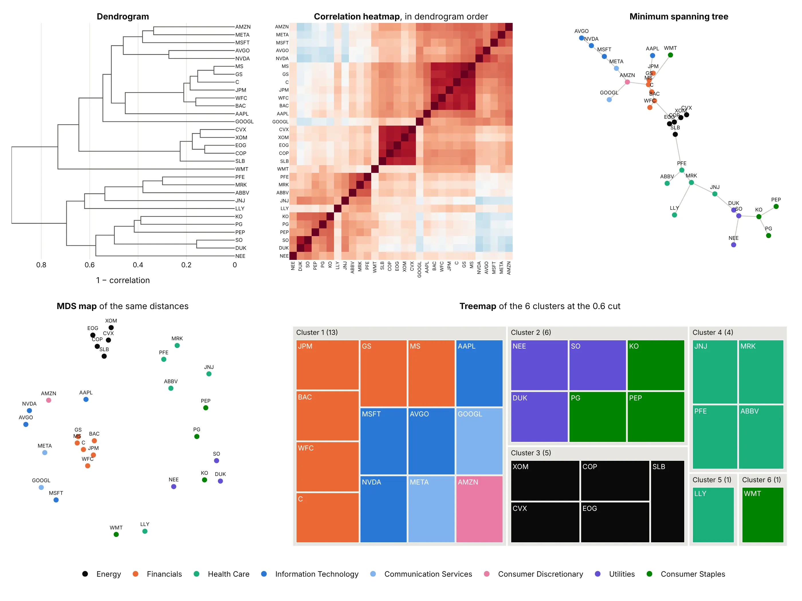
The 30 stocks drawn five ways: the dendrogram, a correlation heatmap ordered by the dendrogram's leaves with dark red blocks for banks and energy, a minimum spanning tree network colored by sector, an MDS map with the sectors as separate clouds, and a treemap of the six clusters at the 0.6 cut

Heatmap of the distance or correlation matrix, ordered by the tree (works too, and better for exact values). Every pair's correlation is visible, and ordering the rows by the dendrogram turns clusters into dark blocks. Put the dendrogram on its edges and you have a clustered heatmap.
Minimum spanning tree network graph (different). It keeps only the strongest link for each stock, which shows chains like Amazon to Meta to Microsoft, but you lose the merge heights.
MDS map (different). Multidimensional scaling places items in 2D so that distances roughly match, which shows how far apart whole groups are; the axes have no meaning, and some distances are always distorted.
Treemap or icicle chart of the clusters (worse for clustering). Once you've cut the tree, nested rectangles show cluster membership and sizes, but every merge height is gone.
A table of cluster assignments (worse for exploring). It's what you hand to the next step of an analysis, but it hides how tight each cluster is and what's close to what.

How to make a dendrogram

With AI

ChatGPT, Claude Code, GitHub Copilot, Cursor and other AI tools are excellent at writing Plotly code. Name Plotly in the prompt, and say which distance and linkage you want, because the defaults may not suit your data:

Make a plotly dendrogram from returns_2025.csv (columns: date, then one column of daily returns per stock).

- Cluster the stocks (the columns), not the dates: distance = 1 - correlation, average linkage.
- Use plotly.figure_factory.create_dendrogram, horizontal, with the tickers as labels on the right.
- Color the clusters below a cut at 0.6 with color_threshold and draw the cut as a dashed line.
- Title the distance axis "1 − correlation" and start it at 0.
- Check: print each stock's cluster number from scipy's fcluster at the same cut.

With Plotly Studio

Plotly Studio is a desktop app where you point an AI at a dataset and it builds charts and a Dash app around your questions. Ask for a dendrogram the same way:

Show a dendrogram of the stocks clustered by the correlation of their daily returns, average linkage, with the clusters colored below a cut and a slider to move the cut and see the clusters change.

Make a dendrogram in Python or JavaScript

This is the code AI tools write under the hood. In Python, create_dendrogram takes one row per item, computes the distances with distfun, clusters them with linkagefun and draws the tree. Its defaults are Euclidean distance and complete linkage, so set both:

import pandas as pd
import plotly.figure_factory as ff
from scipy.cluster.hierarchy import fcluster, linkage
from scipy.spatial.distance import pdist

returns = pd.read_csv("returns_2025.csv", index_col="date")  # one column of daily returns per stock
X = returns.T.to_numpy()  # one row per stock: the things to cluster are the rows

fig = ff.create_dendrogram(
    X, labels=returns.columns.tolist(), orientation="left",
    distfun=lambda x: pdist(x, "correlation"),  # 1 - correlation between stocks
    linkagefun=lambda d: linkage(d, "average"),
    color_threshold=0.6,  # color the clusters that merge below 0.6
)
fig.update_layout(width=800, height=600, xaxis_title="1 − correlation")
fig.show()

# the cluster of each stock if you cut the tree at 0.6
clusters = fcluster(linkage(pdist(X, "correlation"), "average"), t=0.6, criterion="distance")
print(dict(zip(returns.columns, clusters)))

orientation can be "bottom" (the default, leaves along the bottom), "top", "left" or "right"; horizontal trees keep long labels readable. The Plotly dendrogram documentation shows how to put one on the side of a heatmap.

In JavaScript, you can make a dendrogram with plotly.js from a single line trace: cluster the items, then draw each merge as a ∩ shape from the two branches' heights up to the merge height. This version clusters nine stocks with average linkage:

<div id="chart"></div>
<script src="https://cdn.plot.ly/plotly-4.1.1.min.js"></script>
<script>
  // Correlations of 2025 daily returns (Yahoo Finance adjusted closes)
  const names = ["XOM", "CVX", "JPM", "GS", "MS", "NVDA", "AVGO", "DUK", "SO"];
  const corr = [
    [1, .86, .36, .36, .35, .17, .14, .10, .15], [.86, 1, .42, .41, .40, .27, .22, .05, .13],
    [.36, .42, 1, .83, .82, .47, .42, 0, .04], [.36, .41, .83, 1, .91, .57, .54, -.06, 0],
    [.35, .40, .82, .91, 1, .58, .56, -.05, -.03], [.17, .27, .47, .57, .58, 1, .73, -.28, -.26],
    [.14, .22, .42, .54, .56, .73, 1, -.23, -.20], [.10, .05, 0, -.06, -.05, -.28, -.23, 1, .84],
    [.15, .13, .04, 0, -.03, -.26, -.20, .84, 1]];

  // Average-linkage clustering on 1 - correlation
  let clusters = names.map((n, i) => ({leaves: [i], height: 0, kids: null}));
  const dist = (a, b) => {
    let s = 0;
    for (const i of a.leaves) for (const j of b.leaves) s += 1 - corr[i][j];
    return s / (a.leaves.length * b.leaves.length);
  };
  while (clusters.length > 1) {
    let best = [0, 1, Infinity];
    for (let i = 0; i < clusters.length; i++)
      for (let j = i + 1; j < clusters.length; j++) {
        const d = dist(clusters[i], clusters[j]);
        if (d < best[2]) best = [i, j, d];
      }
    const [i, j, d] = best;
    const merged = {leaves: [...clusters[i].leaves, ...clusters[j].leaves], height: d, kids: [clusters[i], clusters[j]]};
    clusters = clusters.filter((_, k) => k !== i && k !== j).concat([merged]);
  }

  // Lay the leaves out left to right, then draw each merge as a ∩ shape
  const order = [], x = [], y = [];
  const place = (c) => {
    if (!c.kids) { c.x = order.length; order.push(names[c.leaves[0]]); return; }
    c.kids.forEach(place);
    const [a, b] = c.kids;
    x.push(a.x, a.x, b.x, b.x, null);
    y.push(a.height, c.height, c.height, b.height, null);
    c.x = (a.x + b.x) / 2;
  };
  place(clusters[0]);

  Plotly.newPlot("chart", [{type: "scatter", mode: "lines", x: x, y: y, line: {color: "#2a78d6", width: 2},
                            hoverinfo: "skip"}], {
    width: 700, height: 450, showlegend: false,
    xaxis: {tickvals: order.map((_, i) => i), ticktext: order, range: [-0.5, order.length - 0.5], showgrid: false},
    yaxis: {title: {text: "1 − correlation"}, rangemode: "tozero"}
  });
</script>

For more than a few hundred items, compute the tree on a server (SciPy's linkage and dendrogram(no_plot=True) return the ∩ coordinates) and send plotly.js the lines.

Make a clustered heatmap with Dash Bio

A clustered heatmap reorders a heatmap's rows and columns by two dendrograms, one on each edge, so similar rows and similar columns end up next to each other. Dash Bio is Plotly's open-source library of bioinformatics charts, and its Clustergram returns that whole figure from a matrix in one call:

import dash_bio
import pandas as pd

genes = pd.read_csv("golub_top40.csv")  # probe, gene, then one column per sample (log2 intensity)

fig = dash_bio.Clustergram(
    data=genes.iloc[:, 2:].to_numpy(), row_labels=genes.gene.tolist(), column_labels=genes.columns[2:].tolist(),
    standardize="row",                                # z-score each gene so the colors compare within a row
    row_dist="correlation", col_dist="correlation", link_method="average",
    color_map=[[0, "#2a78d6"], [0.5, "#ffffff"], [1, "#e34948"]], height=900, width=1100,
)
fig.show()

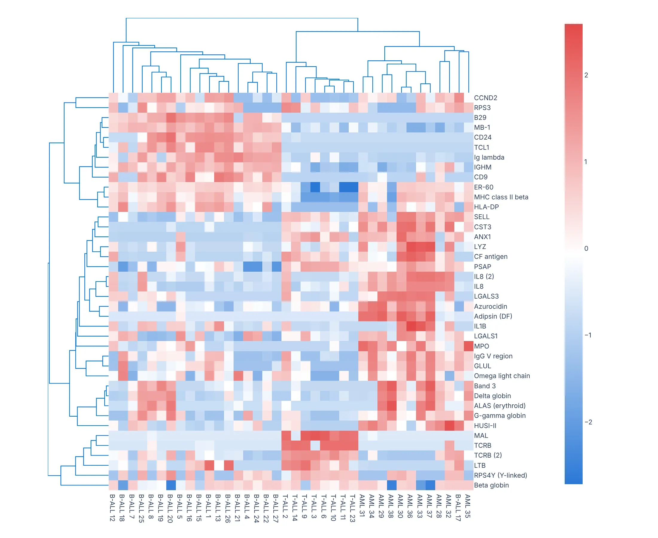
The Golub data drawn by dash_bio.Clustergram: 40 genes by 38 samples with a gene dendrogram on the left and a sample dendrogram on top, samples labeled B-ALL, T-ALL and AML, the same three blocks as the clustered heatmap above and B-ALL 17 among the AML samples

Its link_method defaults to "complete" and the distances to Euclidean, like create_dendrogram. color_threshold, col_group_marker and row_group_marker color and annotate clusters, and in a Dash app a callback can redraw it as readers pick genes, as the Dash Bio example does.

Share it

Every Plotly chart has a Share chart button (the cloud icon in its toolbar) that uploads it to Plotly Cloud and gives you a link. Only you can see it until you change its visibility.

For a live app, put the chart in a Dash app and publish it with the Plotly Cloud CLI. Coding agents can run these commands for you:

pip install "dash[cloud]"
plotly user login
plotly app publish

If your data has to stay in your own cloud or data center, publish to Dash Enterprise instead.

Dos and don'ts

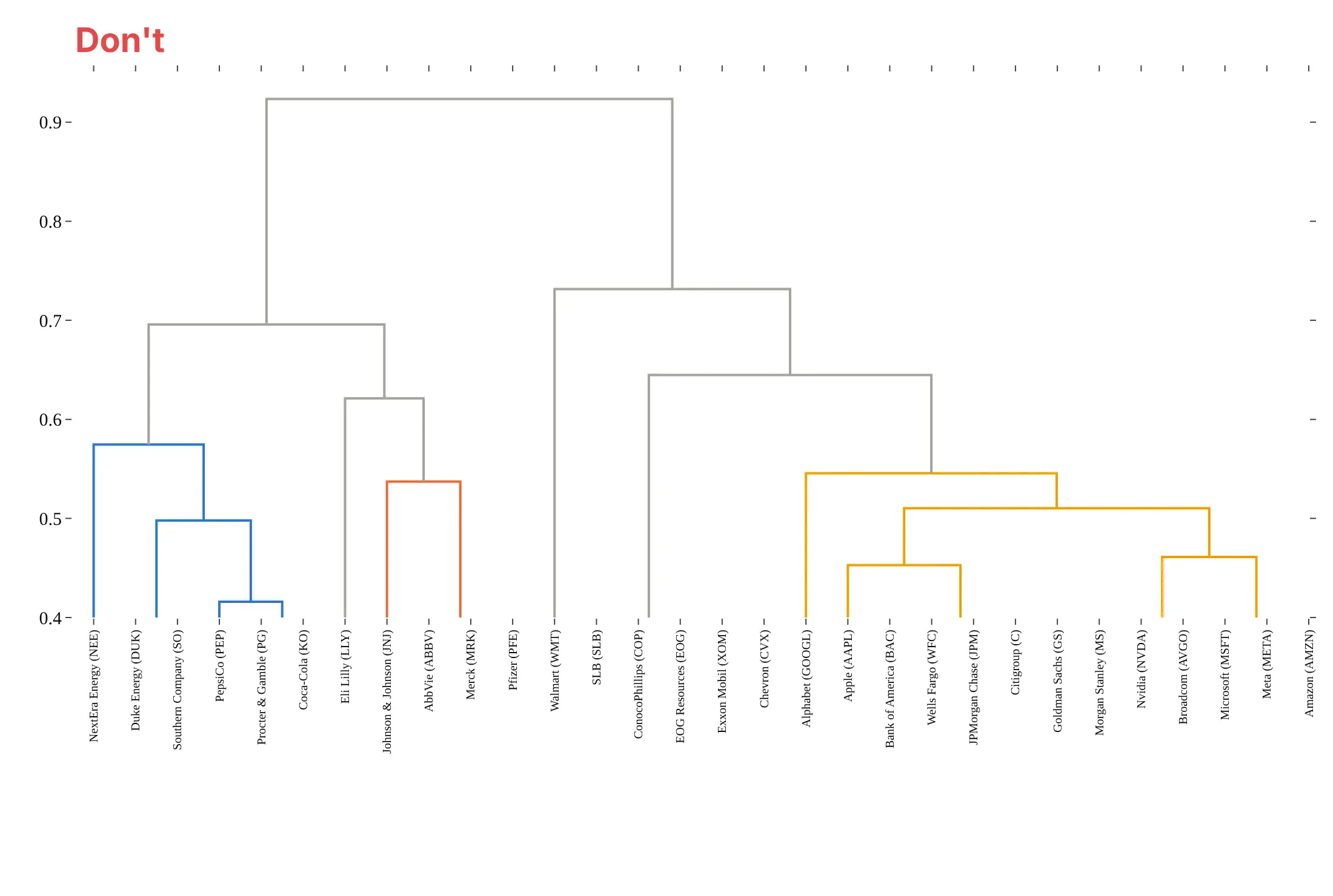
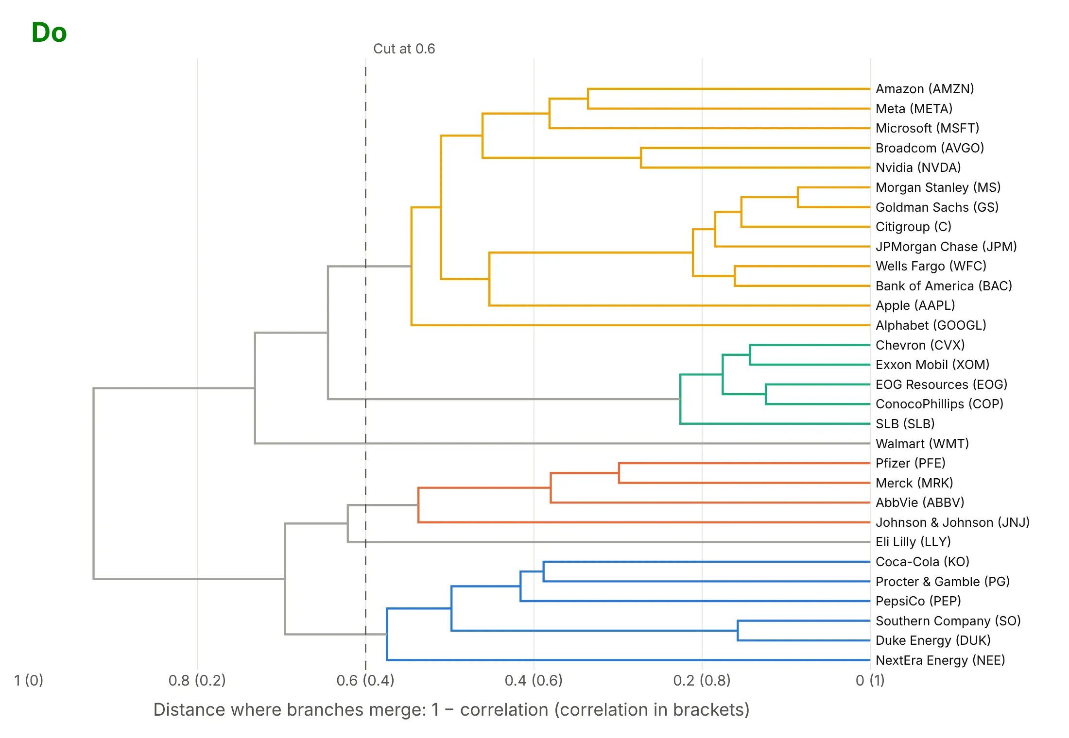
Most of the work in a readable dendrogram is the orientation, the distance axis and the labels. Here are the 30 stocks both ways, with the same clustering and colors.

Don't stand a tree of 30 long names on end with the labels rotated, start the distance axis at 0.4 (which cuts off 16 of the 29 merges, including every tight pair), leave out what the distance is, or use a default serif font:

The 30-stock dendrogram drawn vertically with company names rotated 90 degrees in a small serif font, an untitled y axis from 0.4 to 0.95 that hides every merge below 0.4, so most branches start in mid-air

Do turn it sideways so names read left to right, start the axis at 0 and say in words what the distance is, and draw the cut you used:

The same tree drawn horizontally with readable company names on the right, a distance axis from 0 to 1 labeled 1 minus correlation with the correlation in brackets, and a dashed line at the 0.6 cut

Checklist

Say on the chart which distance and which linkage method you used.
Start the distance axis at 0 and title it in words ("1 − correlation", "substitutions per site").
Draw horizontally when labels are long or there are more than about 20 leaves.
Scale your variables before using Euclidean distance, unless they share units.
Color the clusters from the cut you used, and draw the cut.
Use optimal_leaf_ordering when you want neighbors along the leaves to be similar.

Don't

Read closeness from neighboring leaves; read the height where they join.
Treat the clusters as facts: check that they survive another linkage method or a resample.
Use Ward linkage on correlation or other non-Euclidean distances without converting them first.
Draw thousands of leaves with labels; cut the tree, or switch to a radial layout without names.

Options to customize

A Plotly dendrogram is create_dendrogram (one line trace per merge) or your own line trace, so these are the options that matter most. The full references are the create_dendrogram API reference, SciPy's linkage and Dash Bio's Clustergram.

distfun: the function from rows to a condensed distance matrix; lambda x: pdist(x, "correlation") for 1 − correlation, or return your own precomputed matrix.
linkagefun: the clustering; lambda d: linkage(d, "average") (or "single", "complete", "ward"). The default is complete.
orientation: "bottom", "top", "left" or "right"; sideways for long labels.
labels: the leaf names, in the same order as the rows of X.
color_threshold: the height below which clusters get their own color; links above it share one color.
colorscale: 8 colors for the branches. The first is used for links above the threshold and the clusters take the 3rd, 6th, 2nd, 5th, 8th and 4th in turn, so put your palette in that order.
hovertext: one hover text per merge trace, for example the merge height and the items under it.
scipy.cluster.hierarchy.optimal_leaf_ordering: wrap the linkage in it so adjacent leaves are as similar as possible.
scipy.cluster.hierarchy.fcluster: the cluster number of each item at a height (criterion="distance") or for a number of clusters (criterion="maxclust").
fig.update_traces(line_width=...) and axis range, title, side: the line width, the distance axis from 0 with a title, and labels on the side the tree points to.
dash_bio.Clustergram(standardize=..., row_dist=..., col_dist=..., link_method=..., color_threshold=..., optimal_leaf_order=...): the same choices for a clustered heatmap, for rows and columns separately.

More dendrogram examples

Six more dendrograms built from real public data, each with its source, the technique that makes it work and a prompt to rebuild it.

1. mtcars, R's classic car dataset

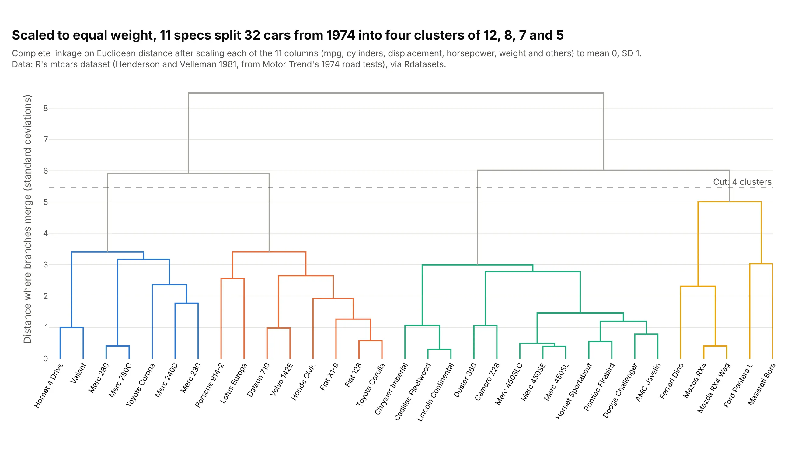
Vertical dendrogram of 32 cars from Motor Trend's 1974 road tests clustered on 11 standardized specs with complete linkage, cut into four colored clusters: 12 V8 cars such as the Cadillac Fleetwood and Camaro Z28, 8 small four-cylinder cars such as the Honda Civic and Fiat 128, 7 mid-size sedans such as the Merc 280 and Valiant, and 5 sports cars including the Ferrari Dino and Maserati Bora

R's mtcars table holds 11 specs for 32 cars that Motor Trend tested in 1974. After scaling each column, complete linkage cut into four clusters gives 12 V8 cars averaging 15.0 miles per gallon, 8 small four-cylinder cars averaging 28.1, 7 mid-size sedans and 5 sports cars. Data: R's mtcars dataset (Henderson and Velleman 1981, from Motor Trend, 1974), via Rdatasets.

Tip: scale the columns before clustering whenever they're in different units.

Get the data from R's mtcars dataset (the Rdatasets CSV at vincentarelbundock.github.io/Rdatasets/csv/datasets/
mtcars.csv; Motor Trend's 1974 road tests of 32 cars), shaped as a table (columns: car, mpg, cyl, disp, hp, drat,
wt, qsec, vs, am, gear, carb).

Build a plotly dendrogram with create_dendrogram: columns scaled to mean 0 and SD 1, complete linkage, car names as
rotated labels, the four clusters colored with color_threshold and the cut drawn as a dashed line.

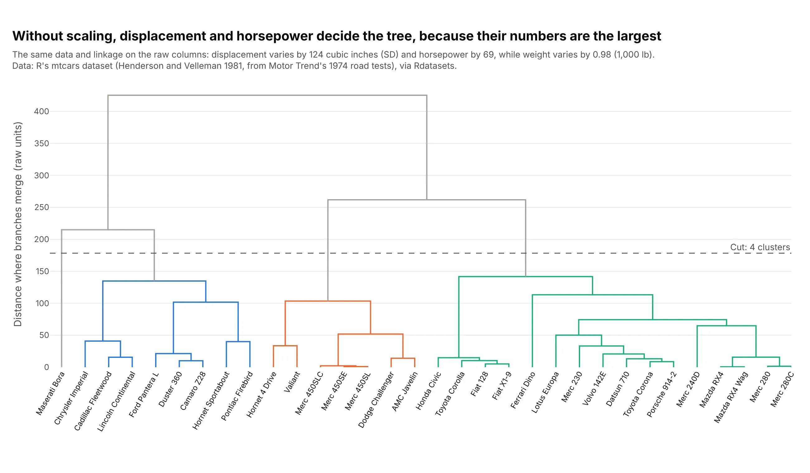
Another way to see it: without scaling, displacement (which varies by 124 cubic inches) and horsepower (69) decide the tree, while weight (0.98 thousand pounds) and the other columns barely count, so the Ferrari Dino lands with the small sedans and the Maserati Bora sits alone.

The same dendrogram on the raw columns: the Maserati Bora on its own, the big V8s in one cluster, the Merc 450 models with the Dodge Challenger and AMC Javelin in another, and the Ferrari Dino and both Mazda RX4s among 16 smaller cars

2. The Treasury yield curve

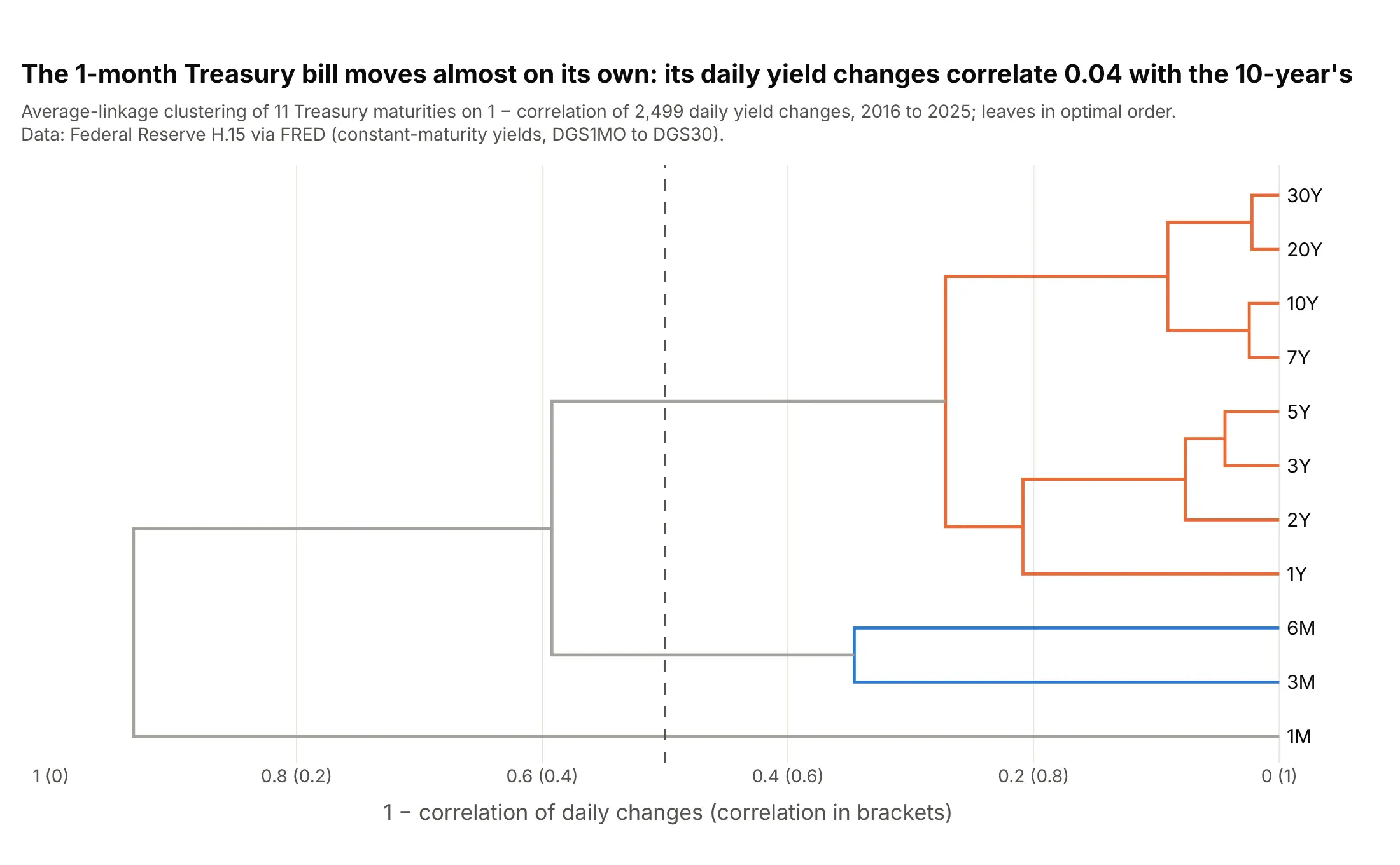
Horizontal dendrogram of 11 Treasury maturities clustered on the correlation of their daily yield changes from 2016 to 2025: 7 and 10 years and 20 and 30 years merge first, 1 to 30 years form one orange cluster, 3 and 6 months a blue one, and the 1-month bill joins last near 0.93

Across 2,499 days from 2016 to 2025, daily moves in 1- to 30-year yields cluster together, the 3- and 6-month bills pair up, and the 1-month bill joins last: its changes correlate only 0.04 with the 10-year's. Data: Federal Reserve H.15 via FRED.

Tip: with a natural order like maturities, use optimal_leaf_ordering so the leaves come out as close to that order as the tree allows.

Get the data from FRED (Federal Reserve H.15 constant-maturity Treasury yields, series DGS1MO, DGS3MO, DGS6MO, DGS1,
DGS2, DGS3, DGS5, DGS7, DGS10, DGS20, DGS30, daily) and shape it into a table of daily changes in basis points,
2016-2025 (columns: date, 1M, 3M, 6M, 1Y, 2Y, 3Y, 5Y, 7Y, 10Y, 20Y, 30Y).

Build a plotly dendrogram of the maturities: 1 - correlation, average linkage with optimal leaf ordering,
horizontal, clusters below 0.5 colored and the distance axis labeled with the matching correlation.

3. Countries by electricity mix, cut into five systems

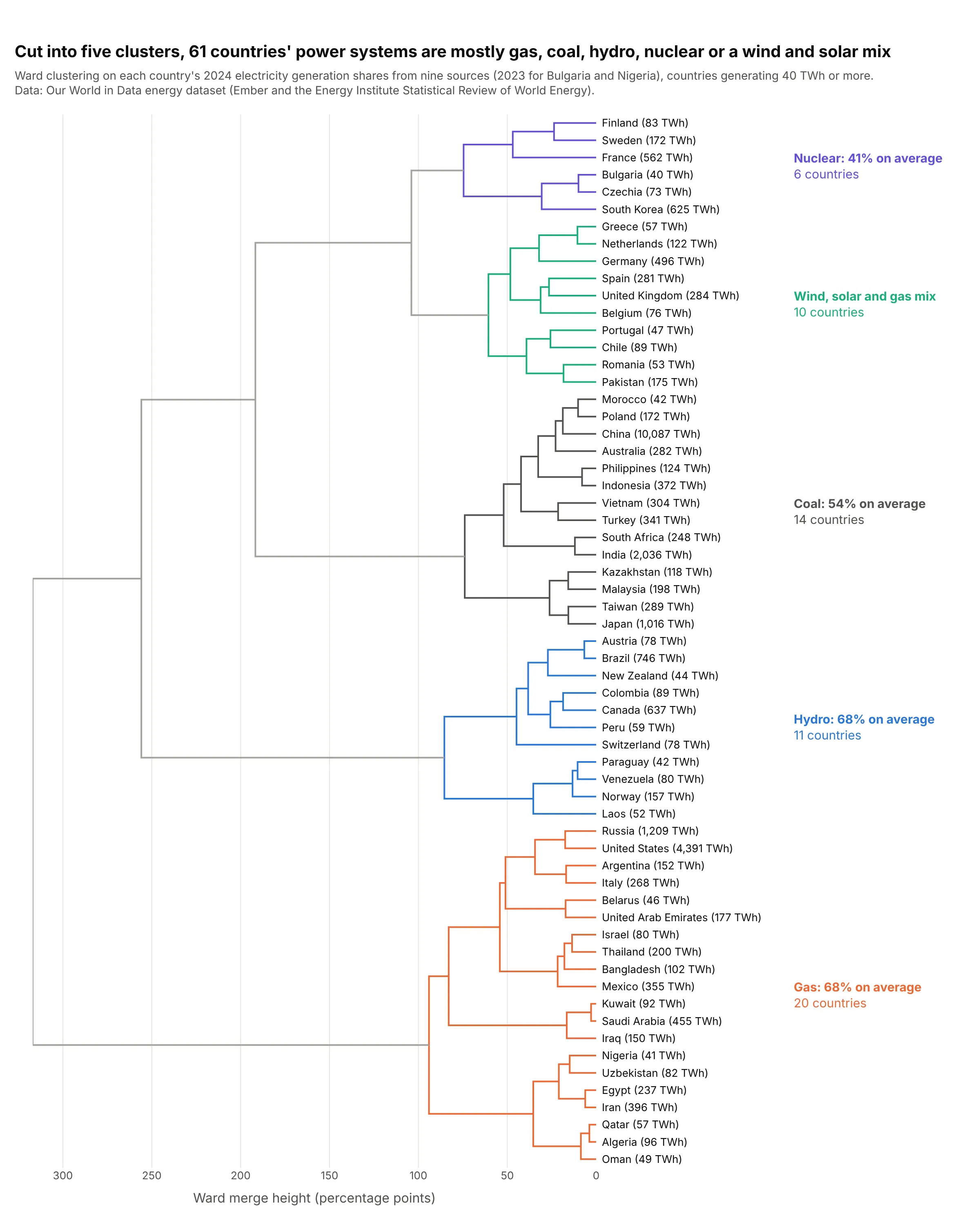
Horizontal dendrogram of 61 countries clustered on their 2024 electricity generation shares with Ward linkage, cut into five colored clusters labeled nuclear 41% on average (6 countries), wind, solar and gas mix (10), coal 54% (14), hydro 68% (11) and gas 68% (20)

Ward clustering of the shares of nine sources in each country's 2024 electricity splits 61 countries into gas (20 countries, 68% gas on average), coal (14), hydro (11), nuclear (6) and a wind, solar and gas mix (10). Data: Our World in Data energy dataset (Ember and the Energy Institute Statistical Review).

Tip: label each cluster with what defines it, here its largest source and average share, so readers don't have to read 61 names.

Get the data from Our World in Data's energy dataset (owid-energy-data.csv on GitHub, from Ember and the Energy
Institute) and shape it into one row per country for 2024, countries generating at least 40 TWh (columns: country,
iso_code, generation_twh, coal, gas, oil, nuclear, hydro, wind, solar, bioenergy, other_renewables, as % shares).

Build a plotly dendrogram: Ward linkage on the shares, horizontal with 61 country names, cut into 5 clusters, each
cluster colored and labeled with its largest source and that source's average share.

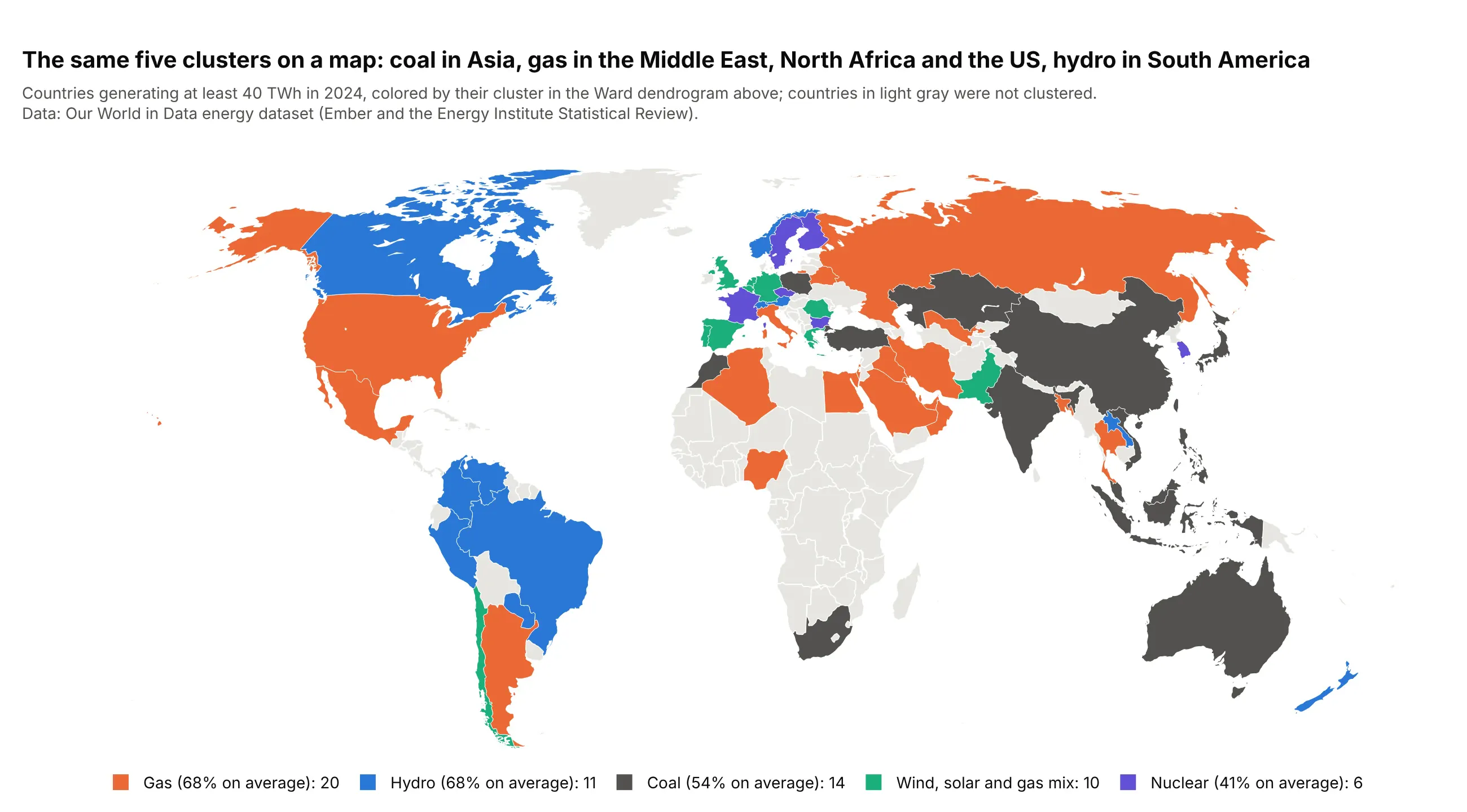
Another way to see it: once you've cut the tree, the clusters are a category you can map, which shows the geography the tree can't.

World map of the five clusters: coal across China, India, Indonesia, Australia and South Africa, gas across the US, Russia, the Middle East and North Africa, hydro across Canada, Brazil and Norway, nuclear in France, Sweden, Finland and South Korea, and the wind and solar mix in Western Europe and Chile

4. A tanglegram of 2008 against 2025

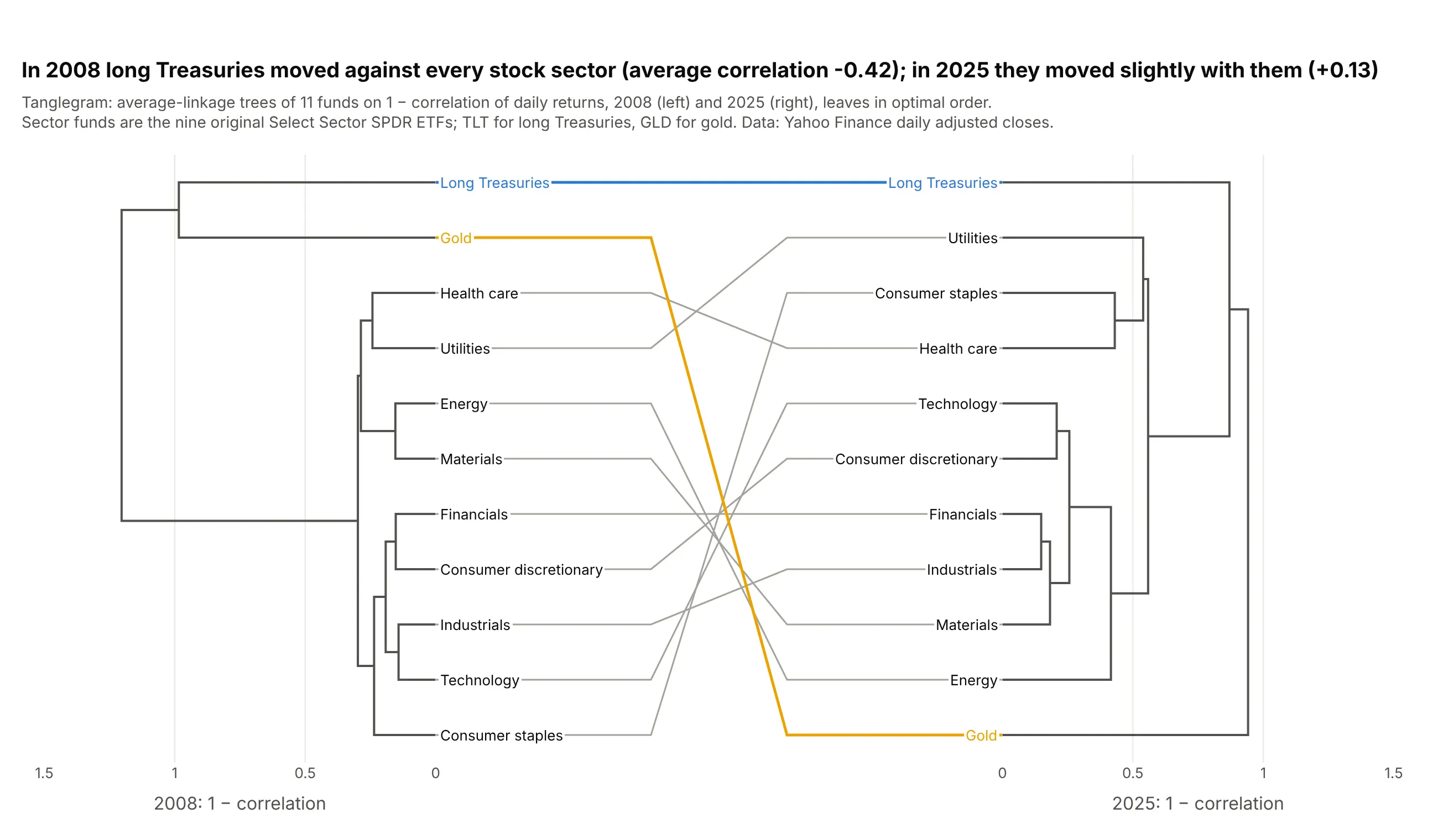
Tanglegram of two dendrograms facing each other, sector ETFs, long Treasuries and gold in 2008 on the left and 2025 on the right, joined by lines: long Treasuries sit far from every sector in 2008 and closer in 2025, and gold moves from beside Treasuries to the bottom

A tanglegram draws two trees of the same items face to face. In 2008 long Treasuries moved against every stock sector, with an average correlation of −0.42, and in 2025 they moved slightly with them (+0.13), so they sit much closer to the sectors in the right-hand tree. Data: Yahoo Finance daily adjusted closes for the nine original Select Sector SPDR ETFs, TLT and GLD.

Tip: put both trees on the same distance scale, or a tight tree and a loose one will look alike.

Get the data from Yahoo Finance's chart API (daily adjusted closes for XLB, XLE, XLF, XLI, XLK, XLP, XLU, XLV, XLY,
TLT and GLD in 2008 and 2025) and shape it into daily returns (columns: date, year, then one per ticker).

Build a plotly tanglegram: one average-linkage dendrogram per year on 1 - correlation with optimal leaf ordering,
the 2008 tree on the left and 2025 mirrored on the right on the same 0 to 1.5 scale, and a line joining each fund
to itself, colored for TLT and GLD.

5. A radial dendrogram of the whole S&P 500

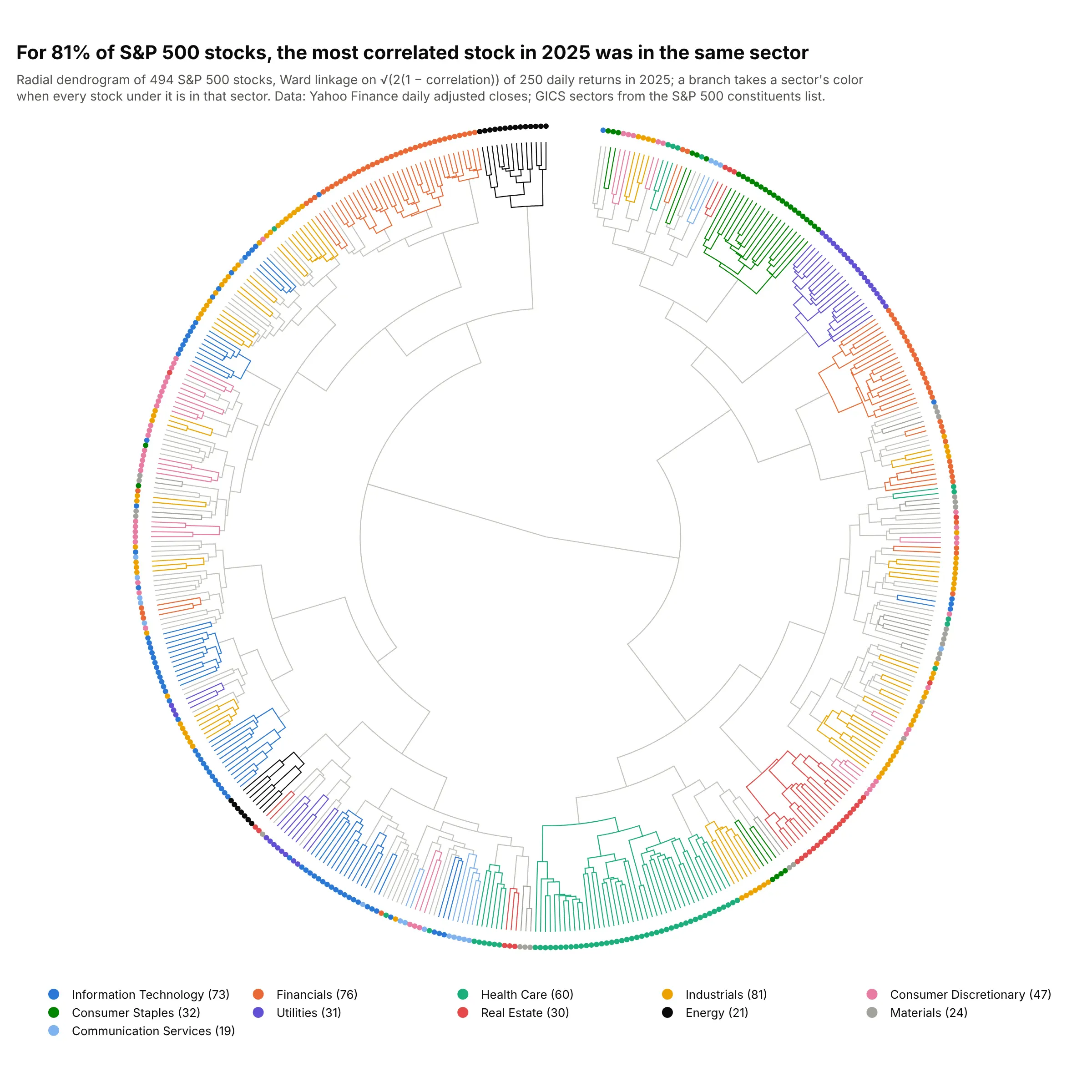
Radial dendrogram of 494 S&P 500 stocks with a ring of dots colored by sector, branches colored when every stock under them shares a sector: large single-color fans for health care, utilities, real estate, financials and energy, and gray mixed branches for industrials and consumer stocks

For 81% of 494 S&P 500 stocks, the stock whose 2025 returns correlated most with theirs was in the same sector. Drawn in a circle, the tree fits every stock in a square image, and cut into 11 clusters, three of them hold a single sector: 19 real estate stocks, 20 utilities and 14 energy stocks. Data: Yahoo Finance daily adjusted closes; GICS sectors from the S&P 500 constituents list.

Tip: for hundreds of leaves, use Ward linkage; average linkage on this data chains 408 of 494 stocks into one cluster.

Get the data from Yahoo Finance's chart API (daily adjusted closes for every current S&P 500 company in 2025) and the
S&P 500 constituents list on GitHub (datasets/s-and-p-500-companies), shaped as daily returns (columns: date, then one
per ticker) plus a table (columns: ticker, company, sector).

Build a plotly radial dendrogram: Ward linkage on sqrt(2 * (1 - correlation)), scipy's dendrogram coordinates
mapped to Scatterpolar lines (angle = leaf position, radius = distance from the root), a ring of dots colored by
sector with the company on hover.

6. The US Senate by roll-call votes

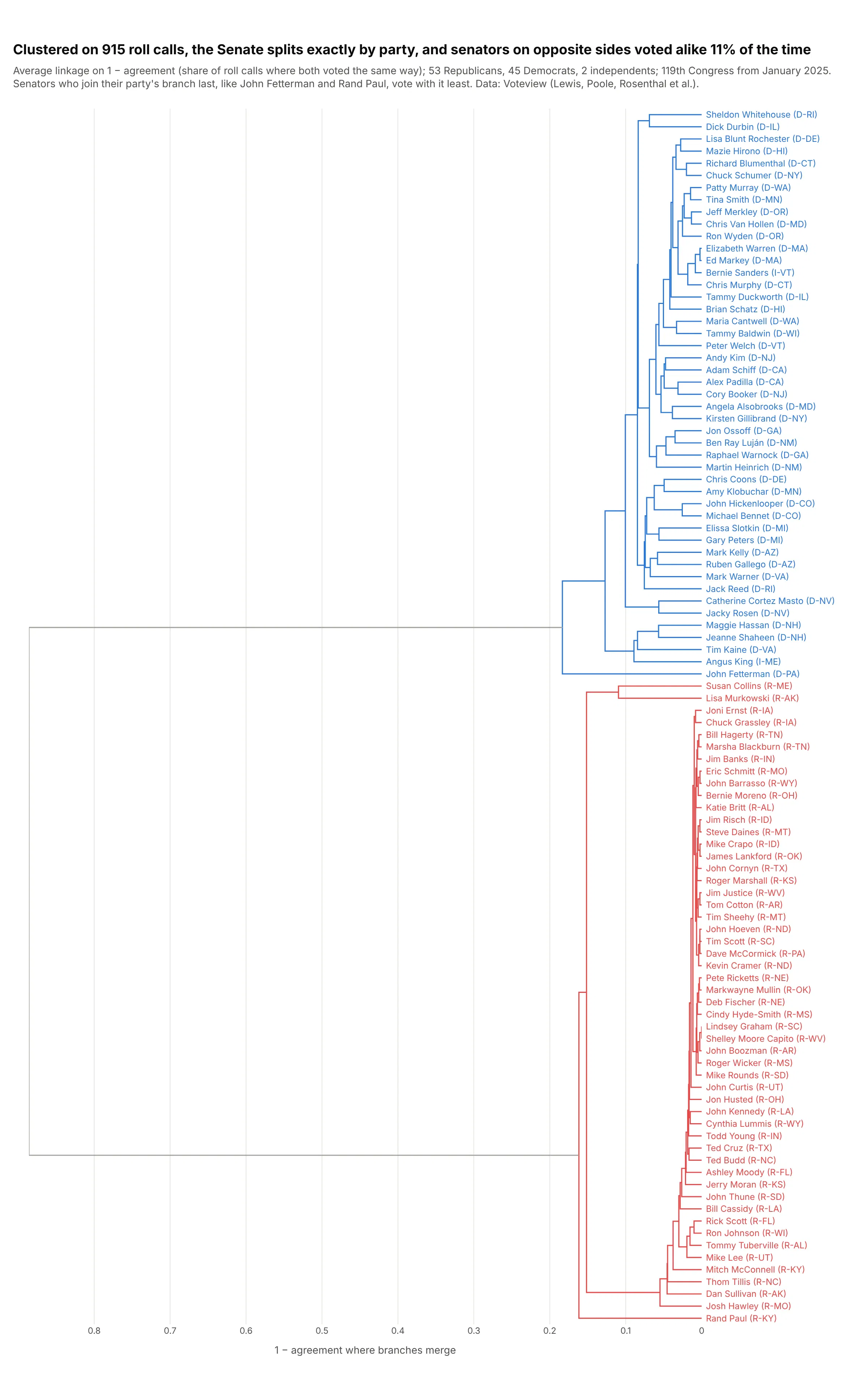
Horizontal dendrogram of 100 senators clustered on how often they voted the same way in 915 roll calls of the 119th Congress: a blue branch of 45 Democrats and 2 independents and a red branch of 53 Republicans that join only at 0.89, with John Fetterman joining the Democrats last and Rand Paul joining the Republicans last

Clustered on 915 roll calls from January 2025 to September 2026, the Senate splits exactly by party, and senators on opposite sides voted alike 11% of the time. John Fetterman and Rand Paul are the last to join their party's branch. Data: Voteview (Lewis, Poole, Rosenthal et al.).

Tip: for votes or survey answers, use agreement over the items both people answered, so missed votes don't count as disagreement.

Get the data from Voteview (S119_votes.csv and S119_members.csv, Senate roll calls of the 119th Congress) and shape
it into an agreement matrix: for each pair of senators, the share of roll calls where both voted and voted the same
way (rows and columns: senators with at least 300 votes).

Build a plotly dendrogram: average linkage on 1 - agreement, horizontal with names like "Rand Paul (R-KY)", names
and branches colored blue for Democrats and independents and red for Republicans.