Chris Parmer

October 24, 2026

Network Graphs - A Complete Guide (with 12 Examples)

TL;DR

A network graph draws things as dots and the connections between them as lines, so clusters, hubs and bridges become visible.
Network graphs are also known as network diagrams, node-link diagrams and network maps, and are similar to Sankey diagrams and adjacency matrices.
Use one when the links are the point: grids, pipelines, payments, supply chains, protein interactions, dependencies and partnerships.
For dense networks of more than a few dozen nodes, an adjacency matrix is often easier to read, and a sorted bar chart is better when you only need to rank the nodes.
You can make a network graph with Plotly from two go.Scatter traces, one for the edges and one for the nodes, with positions computed by networkx. The short make_network helper below does it in one call.

What is a network graph?

Network graphs look like this:

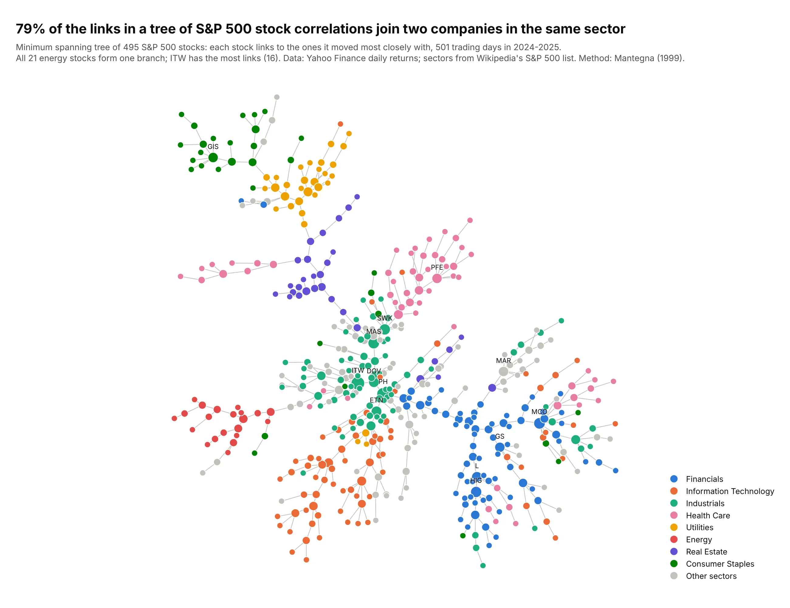
Network graph of 495 S&P 500 stocks as a minimum spanning tree of their daily return correlations in 2024-2025, nodes colored by sector. Utilities, consumer staples, real estate, health care, energy, financials, technology and industrials each form their own branches; 79% of links join two stocks in the same sector and Illinois Tool Works has the most links, 16

Data: Yahoo Finance daily returns, 2024-2025; sectors from Wikipedia's list of S&P 500 companies.

How do you read a network graph? In the example above, notice these things:

Each dot is one S&P 500 stock, colored by its sector, and each gray line links two stocks whose daily returns moved closely together. The chart keeps just enough of the strongest links to connect every stock (a minimum spanning tree), which is why it grows branches and has no loops.
The layout only knows which stocks are linked, so it pulls linked stocks close together without being told their sectors. When one color gathers in one place, the data put it there, as with the red energy stocks that form a single branch at the lower left.
Bigger dots have more links. Illinois Tool Works (ITW), the large green dot near the center, has the most, and the green industrials sit in the middle of the tree, where they take part in about half of the links between sectors.
79% of the links join two stocks in the same sector, so the links that cross sectors are easy to spot. On the left, a branch of pink health care stocks that includes the big health insurers, UnitedHealth among them, hangs off the purple real estate cluster.
Two stocks with no line between them can still move together, because the tree drops every link it doesn't need. How far apart two branches sit on the page is also the layout's choice, so trust the lines more than the distances.

It's often used for charts like these:

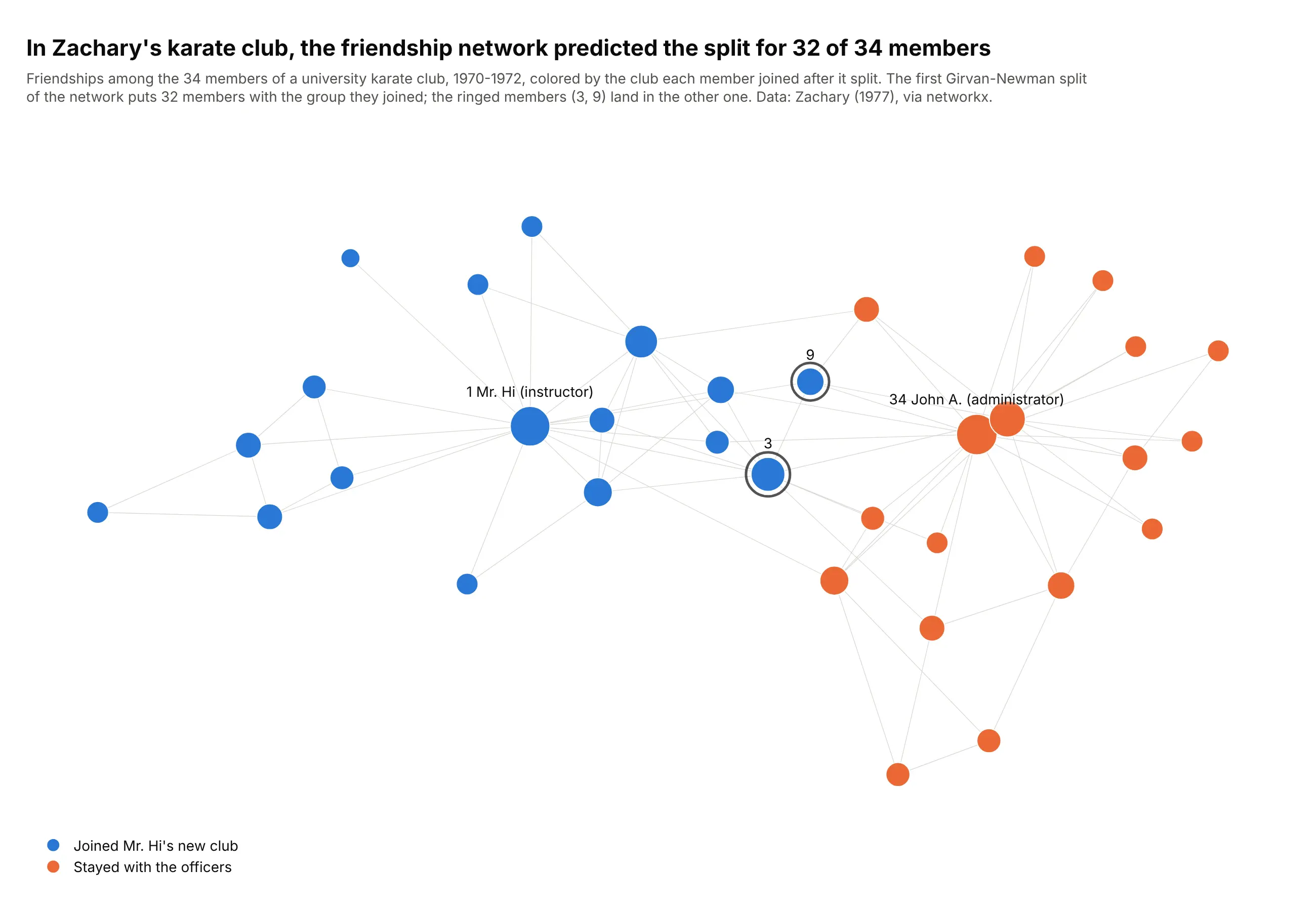
Network graph of the 34 members of Zachary's karate club and their 78 friendships, colored by the club each member joined after the club split: a blue group around the instructor, Mr. Hi (member 1), and an orange group around the administrator, John A. (member 34), with members 3 and 9 ringed

A social network, the textbook example. In Zachary's 1970s study of a university karate club, the network of friendships alone predicted which side of the split 32 of the 34 members joined. Data: Zachary (1977), via networkx.

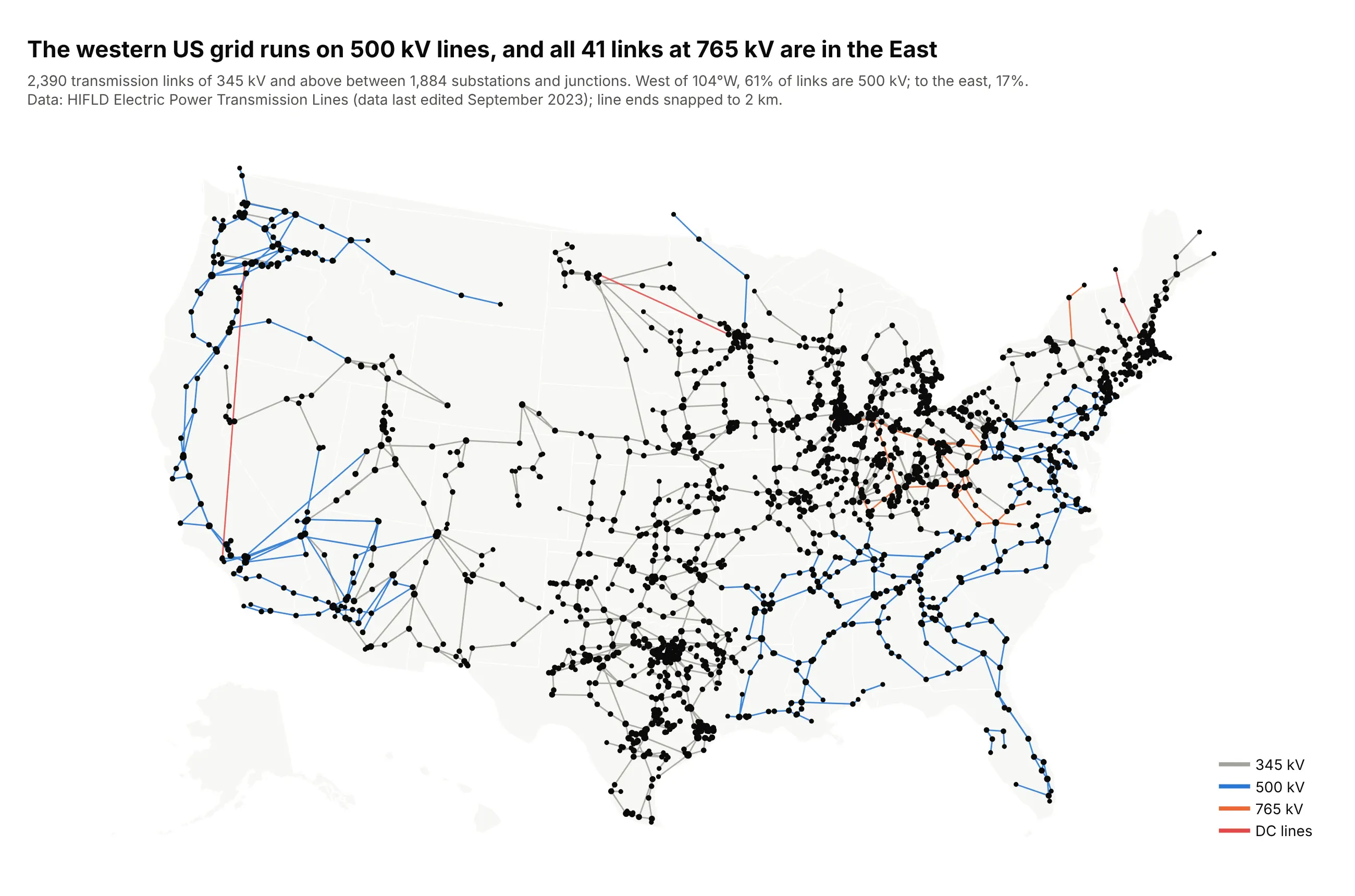
Map of the US transmission grid at 345 kV and above, 2,390 links between 1,884 substations and junctions, colored by voltage: 500 kV lines in blue dominate the West, 765 kV lines in orange run only in the East, and 345 kV lines in gray cover Texas and the Midwest

Infrastructure on a map. When nodes have coordinates, the layout is the map: 61% of extra-high-voltage links west of 104°W are 500 kV lines, against 17% to the east. Data: HIFLD Electric Power Transmission Lines.

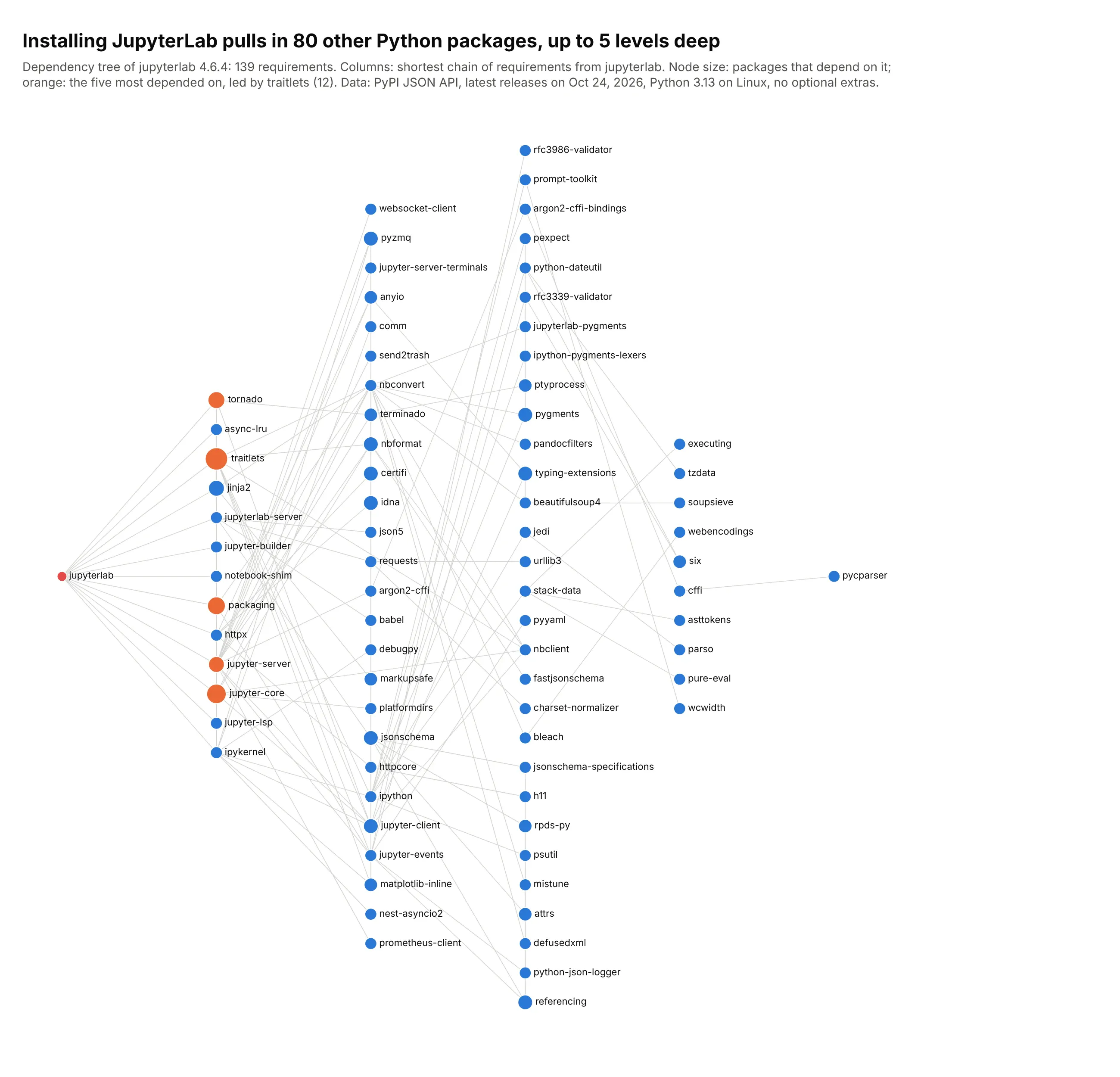
Hierarchical network of the 81 Python packages installed with JupyterLab, in columns by distance from jupyterlab. traitlets, packaging, tornado, jupyter-server and jupyter-core are the largest nodes, and pycparser sits five levels deep

Dependencies. Installing JupyterLab pulls in 80 other packages, and 12 of them require traitlets. Data: PyPI JSON API.

A short history

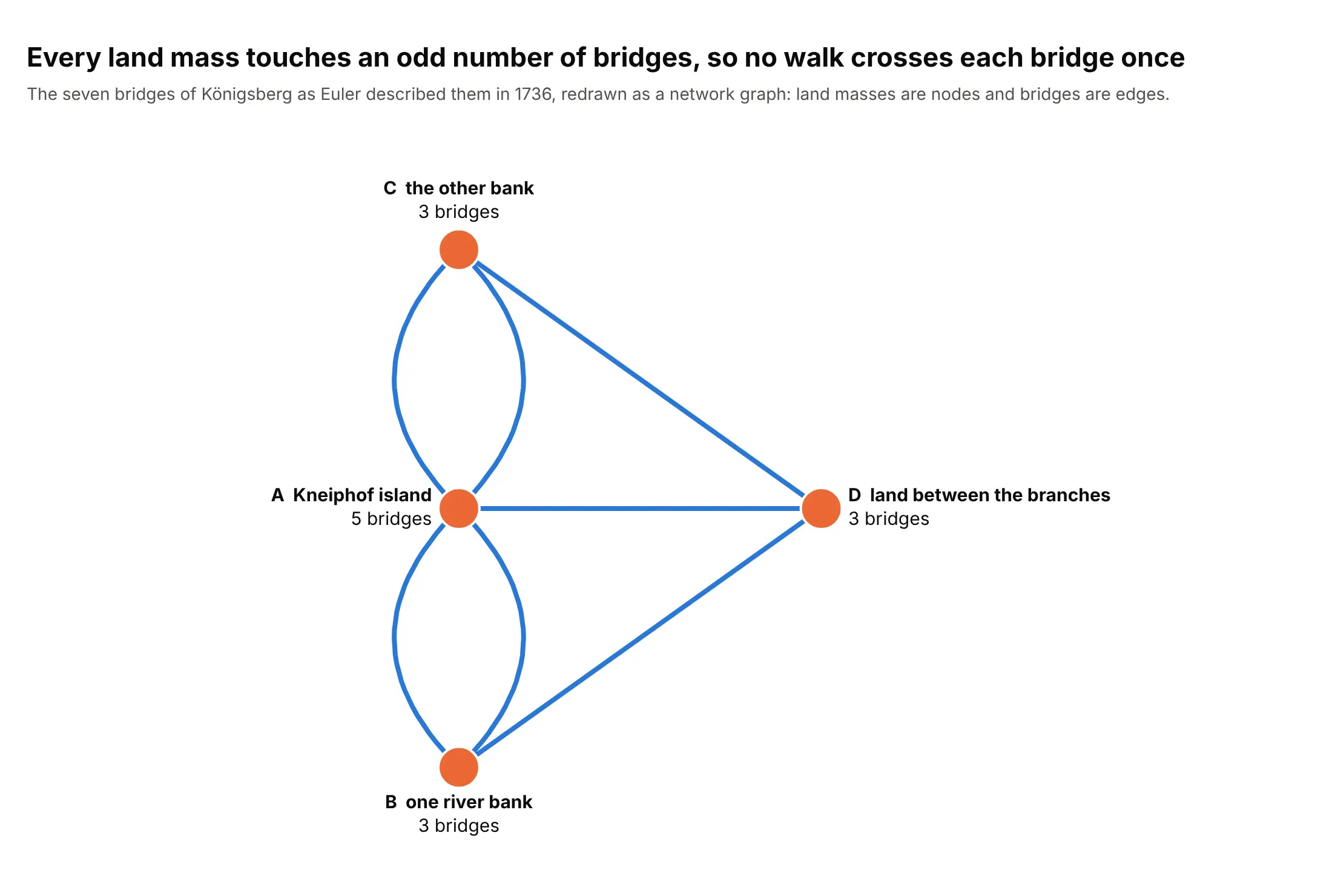
Leonhard Euler started graph theory in 1736 by turning the seven bridges of Königsberg into land masses and the links between them, and proved that no walk crosses every bridge exactly once (Euler Archive, E53):

Euler's seven bridges of Königsberg redrawn as a network graph: the Kneiphof island A with 5 bridges, the two river banks B and C and the land between the branches D with 3 bridges each

Automatic layouts came much later. Force-directed methods such as Kamada and Kawai (1989) and Fruchterman and Reingold (1991) treat edges as springs and nodes as repelling each other. networkx's spring_layout uses Fruchterman and Reingold's method, and kamada_kawai_layout the other.

Alternatives to a network graph

Here's the same bank lending network drawn five ways. Some are better for the question, some worse, some just different:

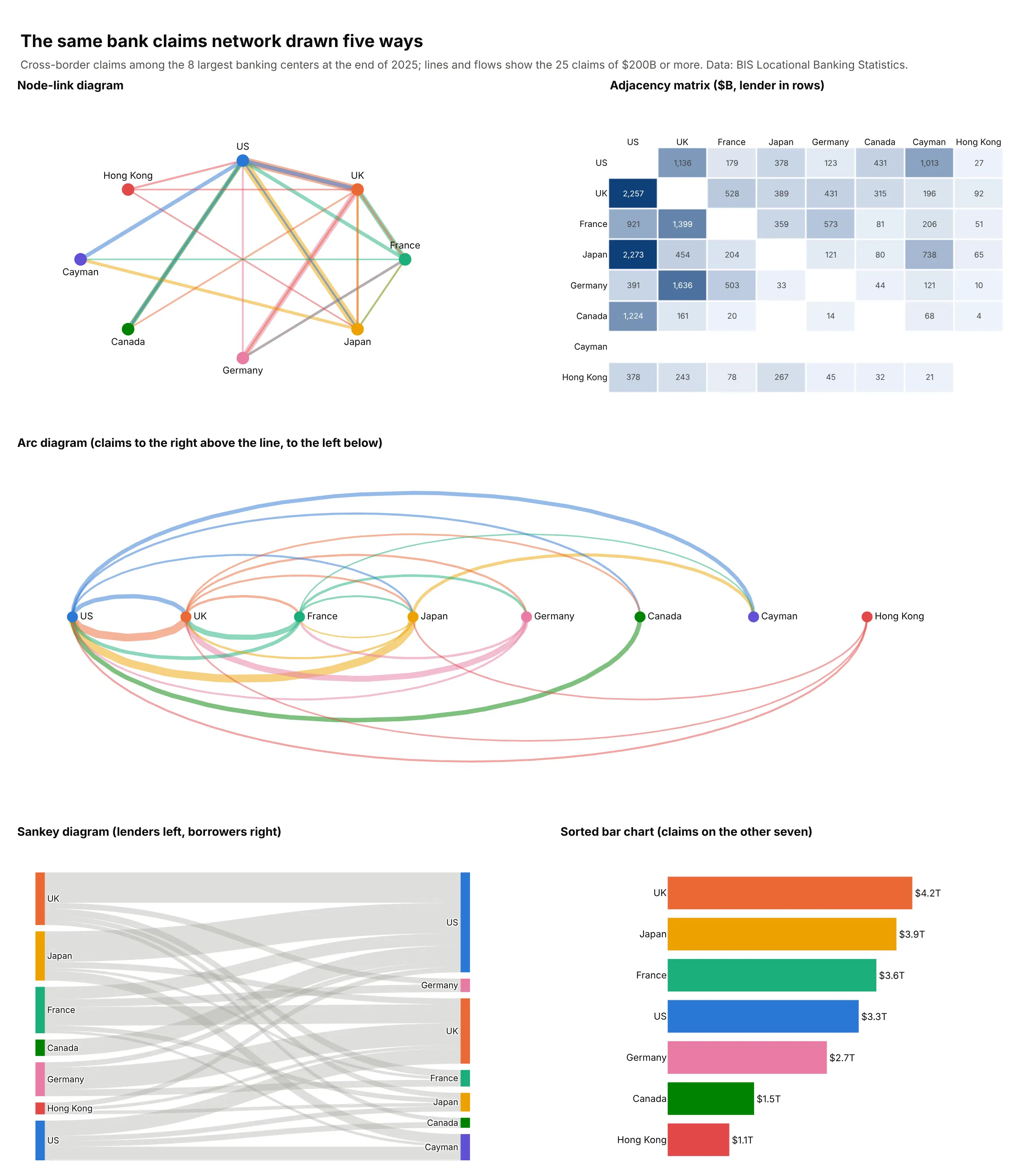
Cross-border bank claims among the eight largest banking centers drawn five ways: a circular node-link diagram, an adjacency matrix with values in billions, an arc diagram with countries on a line, a Sankey diagram from lenders to borrowers, and a sorted bar chart with the UK's banks lending $4.2 trillion to the other seven

Adjacency matrix (better for dense networks). One row and one column per node, with a filled cell for each link, so nothing overlaps and you can read exact values. Ghoniem, Fekete and Castagliola (2004) found matrices easier to read than node-link diagrams for most tasks on graphs larger than about 20 nodes, except for following paths. See our heatmap guide.
Arc diagram (different). Nodes sit on a line and links arc over and under it, which works when the order of the nodes means something, such as time or position on a genome.
Sankey diagram (better for flows between stages). When links carry amounts from sources to destinations, widths add up. See our Sankey diagram guide.
Sorted bar chart (better for ranking nodes). If the question is "which country lends the most", rank the nodes by a measure and drop the links.

How to make a network graph

With AI

ChatGPT, Claude Code, GitHub Copilot, Cursor and other AI tools are excellent at writing Plotly code. Name Plotly and networkx in the prompt, say what nodes and edges are and what size and color mean, and list the checks you want:

Make a plotly network graph from partners.csv (columns: company_a, company_b, shared_trials)
and sponsors.csv (columns: company, trials_led).

- Build the graph with networkx; keep pairs with 3 or more shared trials and only the
  largest connected component.
- Kamada-Kawai layout. Draw all edges in one go.Scatter line trace with None between
  segments, line width in 4 bins by shared_trials, color #a3a29b.
- Nodes in one marker trace, area proportional to trials_led, white outline.
- Label only the 15 biggest nodes; hover shows the company, trials led and partners.
- Hide both axes and lock the aspect ratio (yaxis scaleanchor="x").
- A title that states the main takeaway.
- Print the number of nodes and edges before and after filtering, so I can check them.
- Save it as network.html and as a PNG at 2x scale.

With Plotly Studio

Plotly Studio is a desktop app where you point an AI at a dataset and it builds charts and a Dash app around your questions. Ask for a network graph the same way:

Show a network graph of balancing authorities linked by electricity traded in 2025, with node color for net exports on a red to blue scale centered on zero, line width for energy traded, and a dropdown to pick a region to highlight.

Make a network graph in Python or JavaScript

This is the code AI tools write under the hood. For graph visualization in Python, you compute positions with networkx and draw edges and nodes as two go.Scatter traces. This helper does both, and every example in this guide builds on a fuller version of it:

import networkx as nx
import pandas as pd
import plotly.graph_objects as go


def make_network(G, pos, size=None, color="#2a78d6", labels=None):
    """Edges as one line trace (None between segments), nodes as one marker trace."""
    ex, ey = [], []
    for u, v in G.edges():
        ex += [pos[u][0], pos[v][0], None]
        ey += [pos[u][1], pos[v][1], None]
    nodes = list(G.nodes())
    fig = go.Figure([
        go.Scatter(x=ex, y=ey, mode="lines", line=dict(color="#c3c2bc", width=1), hoverinfo="skip"),
        go.Scatter(x=[pos[n][0] for n in nodes], y=[pos[n][1] for n in nodes],
                   mode="markers+text", hovertext=nodes,
                   text=[(labels or {}).get(n, "") for n in nodes], textposition="top center",
                   marker=dict(size=[size[n] for n in nodes] if size else 10, color=color,
                               line=dict(color="white", width=1))),
    ])
    fig.update_xaxes(visible=False)
    fig.update_yaxes(visible=False, scaleanchor="x")  # keep the layout's proportions
    fig.update_layout(showlegend=False, plot_bgcolor="white")
    return fig


df = pd.read_csv("02_ba_interchange.csv")  # columns: ba, diba, abs_twh, ...
G = nx.from_pandas_edgelist(df, "ba", "diba", edge_attr="abs_twh")
pos = nx.kamada_kawai_layout(G)
deg = dict(G.degree())
fig = make_network(G, pos, size={n: 6 + 3 * d for n, d in deg.items()},
                   labels={n: n for n in G if deg[n] >= 8})
fig.show()

The fuller version in this guide's examples also splits edges into width bins (a line trace has one width), colors edges with a function, scales node area by a value and draws on a map with go.Scattergeo.

In JavaScript, plotly.js takes the same two traces. Put the positions in your data (or compute them with a library such as d3-force) and pass null between edge segments. A JavaScript dependency graph works the same way: give each package a column by its distance from the root, as in the JupyterLab example above, and draw it with these two traces:

<div id="chart"></div>
<script src="https://cdn.plot.ly/plotly-4.1.1.min.js"></script>
<script>
  const nodes = {A: [0, 0], B: [0, -1], C: [0, 1], D: [1.4, 0]};
  const edges = [["A", "B"], ["A", "C"], ["A", "D"], ["B", "D"], ["C", "D"]];
  const ex = [], ey = [];
  for (const [u, v] of edges) {
    ex.push(nodes[u][0], nodes[v][0], null);
    ey.push(nodes[u][1], nodes[v][1], null);
  }
  Plotly.newPlot("chart", [
    {x: ex, y: ey, mode: "lines", line: {color: "#a3a29b", width: 2}, hoverinfo: "skip"},
    {x: Object.values(nodes).map(p => p[0]), y: Object.values(nodes).map(p => p[1]),
     text: Object.keys(nodes), mode: "markers+text", textposition: "top center",
     marker: {size: 24, color: "#2a78d6"}}
  ], {showlegend: false, xaxis: {visible: false}, yaxis: {visible: false, scaleanchor: "x"}});
</script>

Share it

Every Plotly chart has a Share chart button (the cloud icon in its toolbar) that uploads it to Plotly Cloud and gives you a link. Only you can see it until you change its visibility.

For a live app, put the chart in a Dash app and publish it with the Plotly Cloud CLI. Coding agents can run these commands for you:

pip install "dash[cloud]"
plotly user login
plotly app publish

If your data has to stay in your own cloud or data center, publish to Dash Enterprise instead.

Dos and don'ts

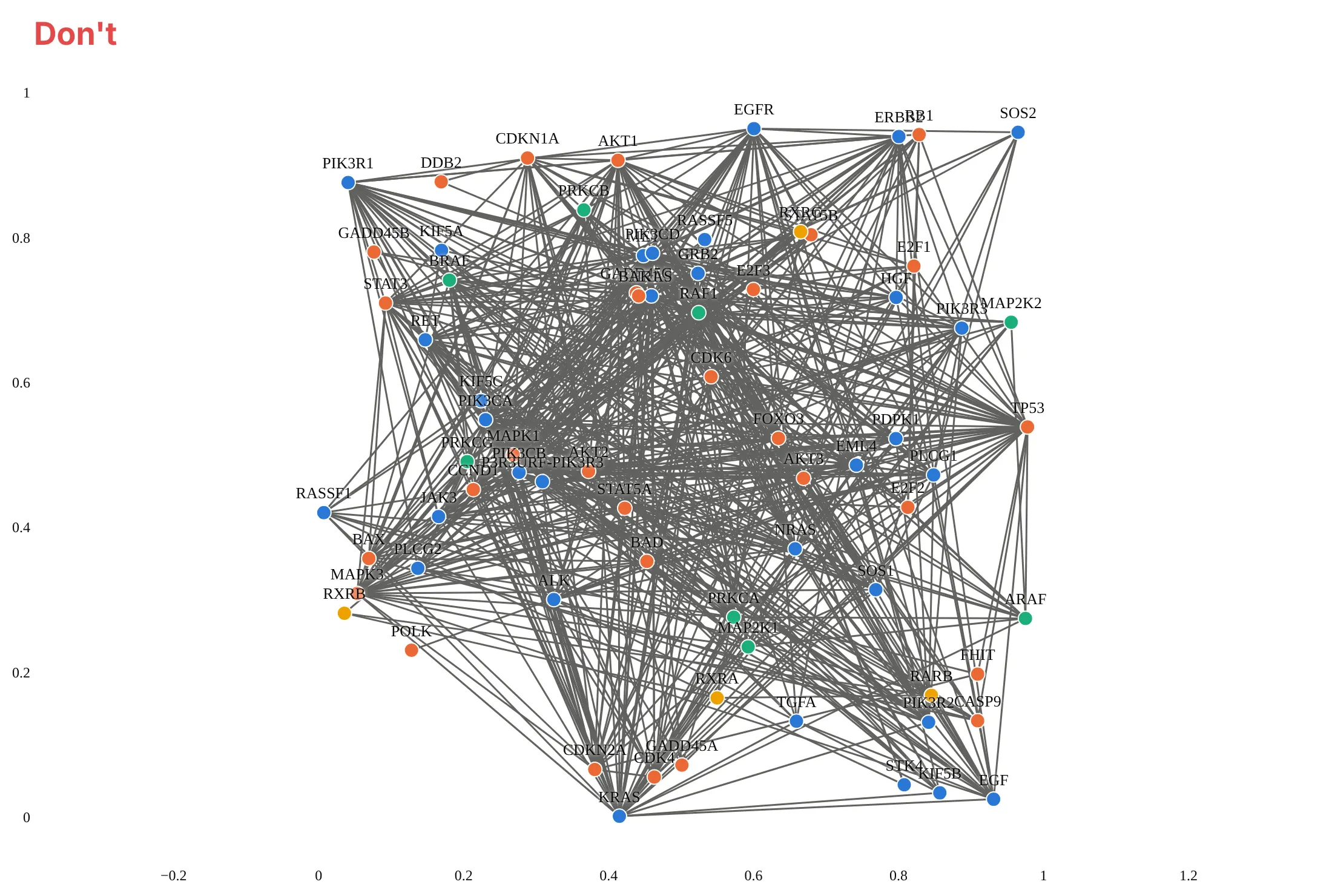
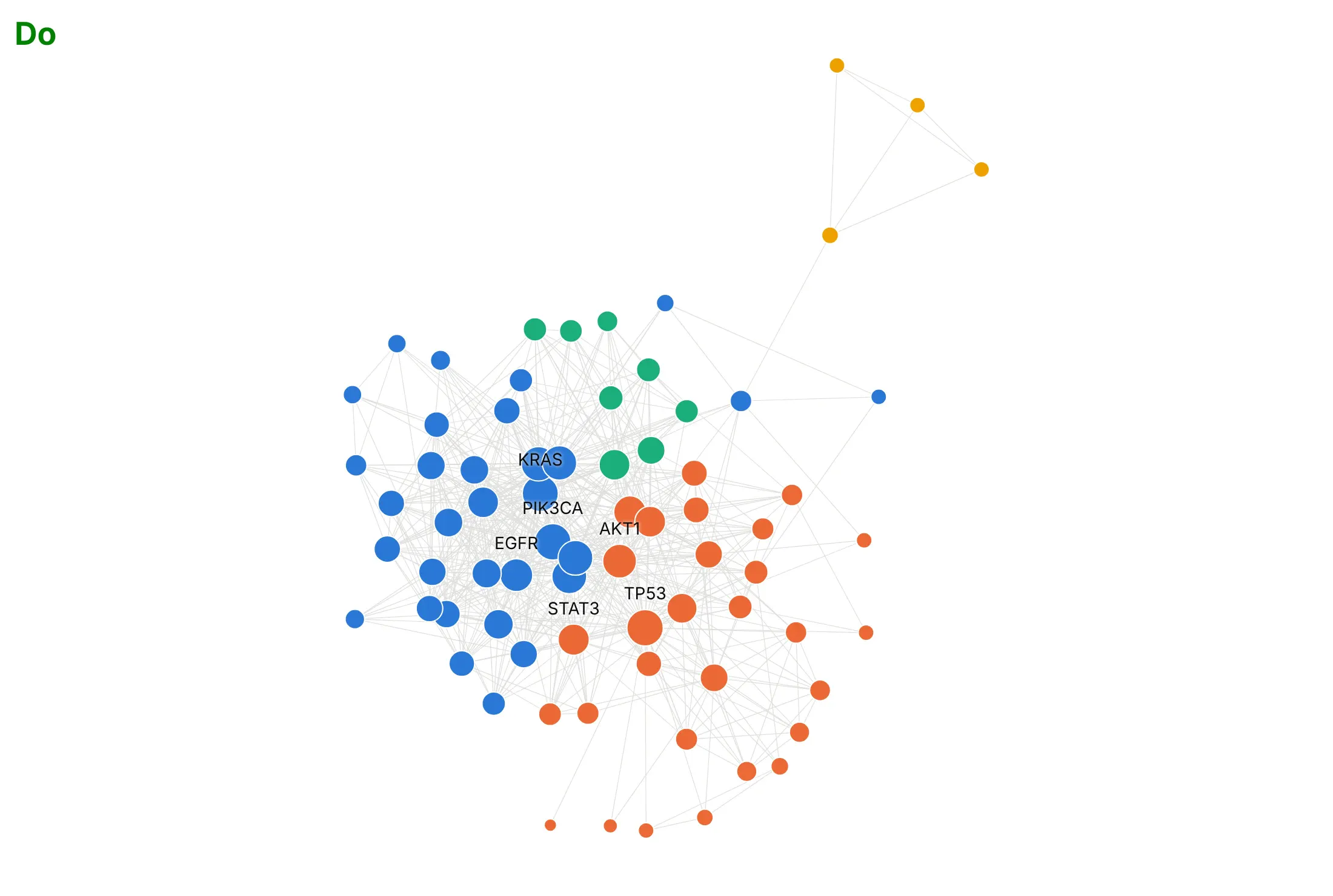
A network graph with every node and link drawn the default way turns into a tangle quickly, so most of the work is choosing the layout and what to exclude. Here is the same protein network both ways, with the same community colors.

Don't use a random layout, leave axes with coordinates that mean nothing, draw heavy dark edges or label every node:

The lung cancer protein network with a random layout, x and y axes from 0 to 1, dark gray edges covering the nodes and overlapping labels on all 73 genes in a serif font

Do use a layout that keeps linked nodes close, draw thin light edges, size nodes by their number of links and label only the hubs:

The same network with a Kamada-Kawai layout, light gray edges, nodes sized by number of interactions, and labels on TP53, PIK3CA, KRAS, AKT1, EGFR and STAT3 only

Use color for one thing

Position already shows the structure and size shows degree, so color is free for one more thing. Here are four options on the same data.

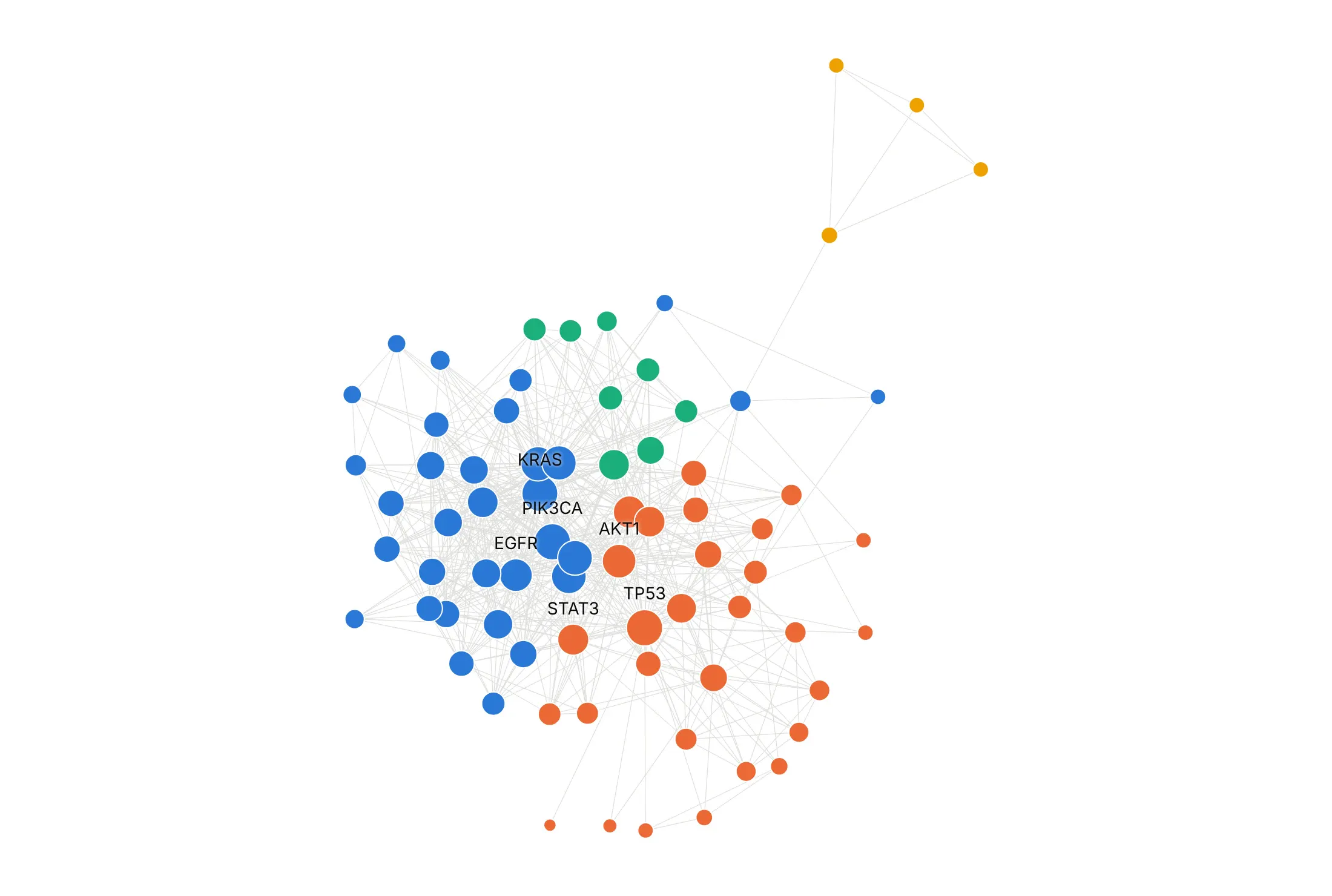
By group. Communities found by modularity: two large groups of 32 and 29 genes, one of 8 and the four retinoid receptors.

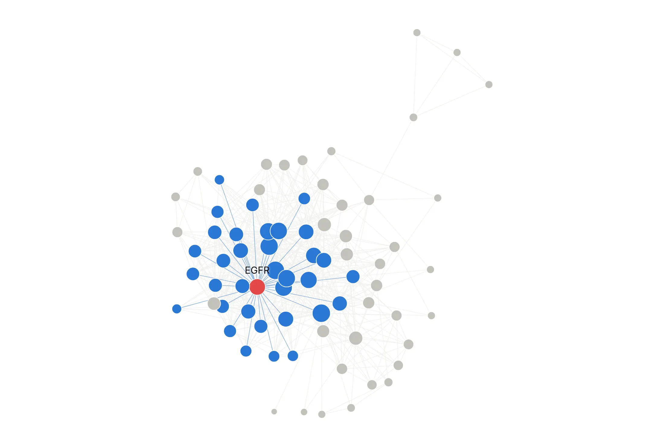
The lung cancer protein network colored by its four communities in blue, orange, green and yellow

Highlight one node. EGFR in red and the 34 proteins it interacts with in blue; the rest in gray.

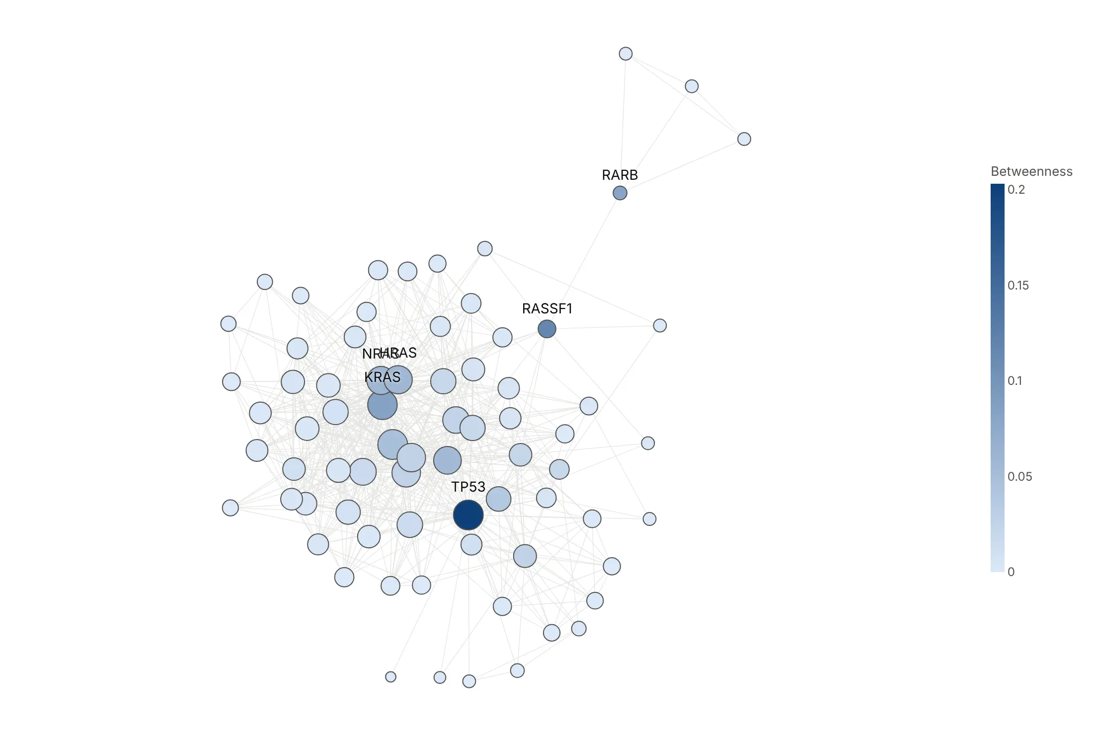
The protein network with EGFR in red, its 34 neighbors and their links in blue and every other node in gray

By a second measure. Betweenness centrality counts how often a node sits on the shortest path between two others: TP53 is highest (0.20), and RASSF1 (0.12) is the bridge to the small group.

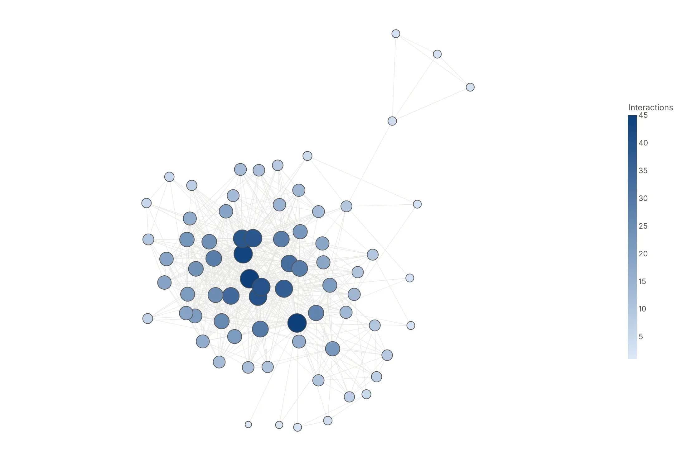
The protein network colored from light to dark blue by betweenness centrality, with TP53 darkest and RASSF1 and RARB standing out at the edges

By degree (avoid). Color repeats what node size already shows.

The protein network shaded by number of interactions, so the biggest nodes are also the darkest

Checklist

Write a title that states the takeaway.
Pick the layout for the data: geography when nodes have places, a hierarchy for trees, a circle for a few nodes in a fixed order, force-directed for everything else.
Draw edges thin and light, in as few traces as possible, and nodes on top.
Hide the axes and lock the aspect ratio with scaleanchor.
Filter before you draw: drop weak links, keep the largest component, or show one node's neighbors.
Fix the layout's random seed so the picture doesn't change on every run.

Don't

Label every node.
Use a random layout or leave the axes on.
Size nodes by radius instead of area.
Draw more than a few thousand edges in a static image without filtering.

Options to customize

Plotly draws network graphs with go.Scatter (and go.Scattergeo on maps), and networkx computes the positions. These are the options that matter most. The full lists are in the Plotly scatter reference and the networkx drawing docs.

go.Scatter(mode="lines") with None separators: all edges in one trace, which is much faster than one trace per edge.
line.width, line.color, opacity: edge emphasis; one trace per width bin when width shows a weight.
go.Scatter(mode="markers"): the nodes, added after the edges so they sit on top.
marker.size: node size; scale by square root so area tracks the value.
marker.color, colorscale, cmid: color by group or by a number; cmid=0 centers a diverging scale.
marker.line: a white outline separates overlapping nodes.
text, textposition, mode="markers+text": labels offset from each marker; leave most labels empty.
hovertext, hovertemplate: names and numbers for every node in the interactive version.
xaxis.visible, yaxis.visible, yaxis.scaleanchor="x": hide coordinates and keep the layout's proportions.
layout.annotations with showarrow, axref="x", ayref="y": arrows for the few edges whose direction matters.
layout.shapes: backgrounds such as a football pitch or region boxes, with layer="below".
go.Scattergeo, geo.scope, geo.projection: networks with real coordinates on a map.
go.Scattergl: WebGL rendering, worth testing for very large networks on machines with a GPU.
nx.spring_layout(G, k, seed, weight): force-directed; k spreads nodes apart, seed makes it repeatable.
nx.kamada_kawai_layout: keeps graph distances, often cleaner for trees and small dense graphs.
nx.circular_layout, nx.shell_layout: nodes on one or more circles, for a few nodes or a hub and spokes.
nx.bipartite_layout, nx.multipartite_layout(subset_key=...): two columns, or one column per level of a hierarchy.

More network graph examples

Seven more network graphs built from real public data, each with its source, the technique that makes it work and a prompt to rebuild it.

1. Power traded between grid operators

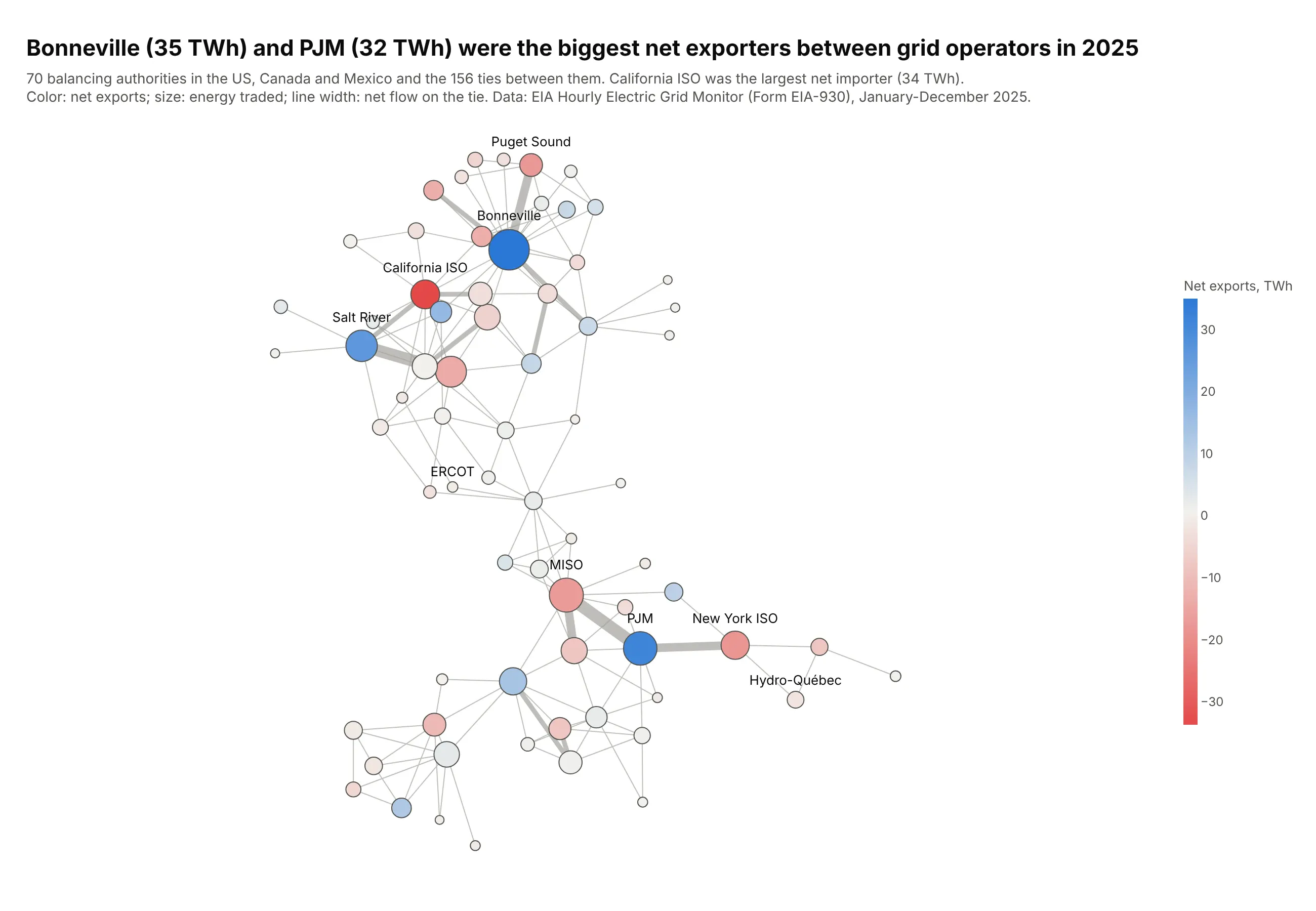
Network of 70 North American balancing authorities and the 156 ties between them in 2025, colored by net exports from red to blue. Bonneville and PJM are dark blue exporters, California ISO is the darkest red importer, and the West and East form two clusters

Each node is a balancing authority, and line width is the net energy that crossed each tie in 2025. Bonneville (35 TWh) and PJM (32 TWh) were the largest net exporters, and California ISO the largest net importer (34 TWh). Data: EIA Hourly Electric Grid Monitor (Form EIA-930).

Tip: a diverging color scale centered on zero (cmid=0) shows exporters and importers at a glance.

Get the data from the EIA Hourly Electric Grid Monitor (Form EIA-930), six-month interchange
files for 2025: hourly MW between each balancing authority and each directly interconnected
one, summed over the year (columns: ba, diba, region, diba_region, net_twh, abs_twh).

Make a plotly network graph with networkx, Kamada-Kawai layout.
- Node color: net exports on a red-white-blue scale with cmid=0; node size: energy traded.
- Edge width in four bins by abs_twh; edges in gray.
- Label the three biggest exporters and importers. Title with the top exporters in TWh.

2. Natural gas pipeline capacity between states

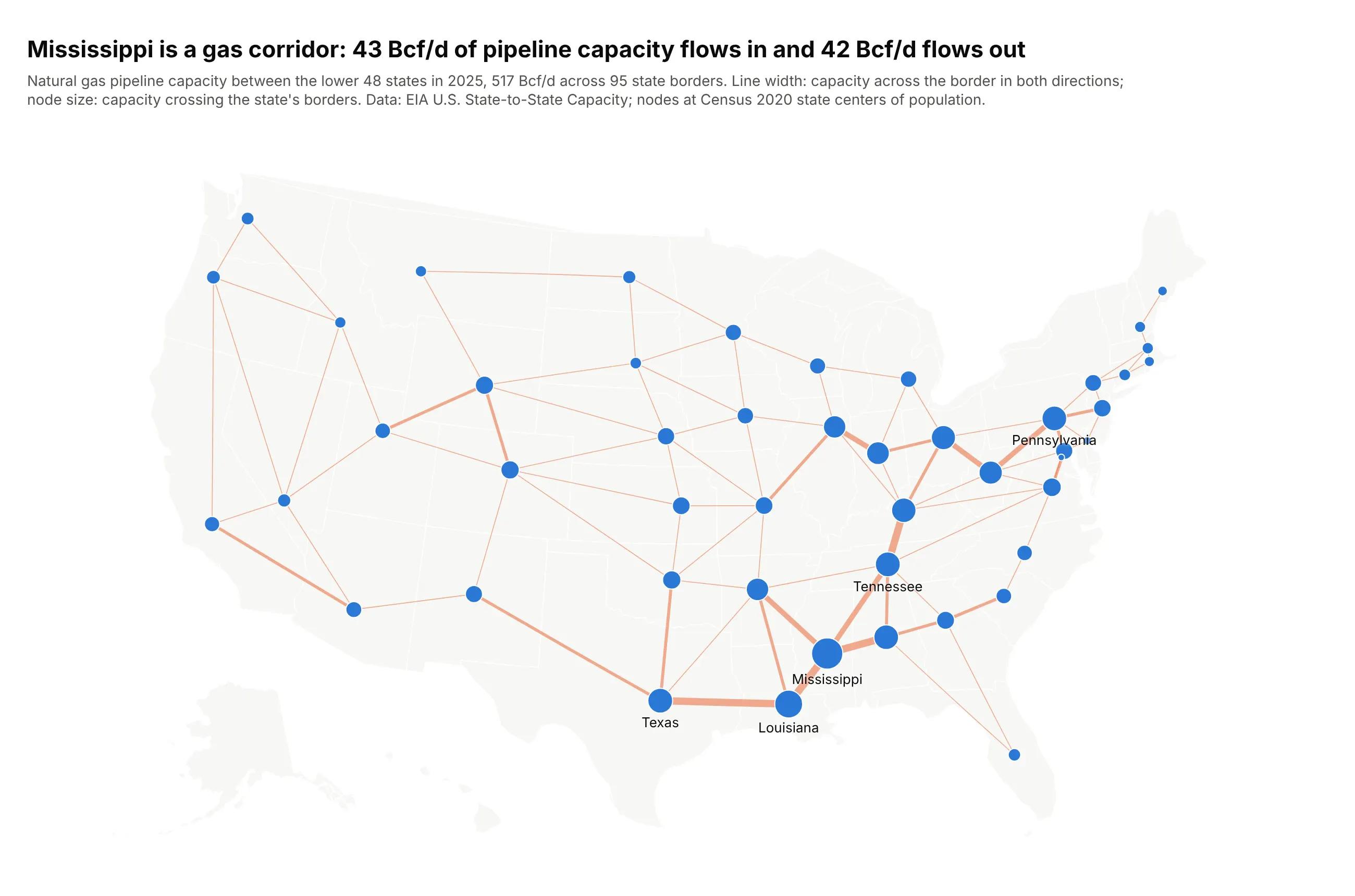
Map of natural gas pipeline capacity between the lower 48 states in 2025, with nodes at each state's center of population. Thick orange lines run from Texas and Louisiana through Mississippi, Alabama and Tennessee to Ohio and Pennsylvania

Line width is the pipeline capacity across each state border in 2025. Mississippi has more capacity crossing its borders than any other state, 43 Bcf/d in and 42 Bcf/d out, and the thickest lines on the map run through it from Louisiana to Alabama and Tennessee. Data: EIA U.S. State-to-State Capacity; Census 2020 centers of population.

Tip: for a map, place each node at a meaningful point such as the center of population, and say so in the subtitle.

Get the data from the EIA "U.S. State-to-State Capacity" workbook (sheet Pipeline State2State
Capacity, 2025) summed by direction for the lower 48 states, and the Census Bureau's 2020
centers of population by state (columns: state_from, state_to, capacity_bcfd, pipelines,
lat_from, lon_from, lat_to, lon_to).

Make a plotly network graph on a go.Scattergeo map (scope usa, albers usa projection).
- One edge per state pair, width in four bins by capacity in both directions.
- Node size: capacity crossing the state's borders; label the top six states.

3. Cross-border bank lending

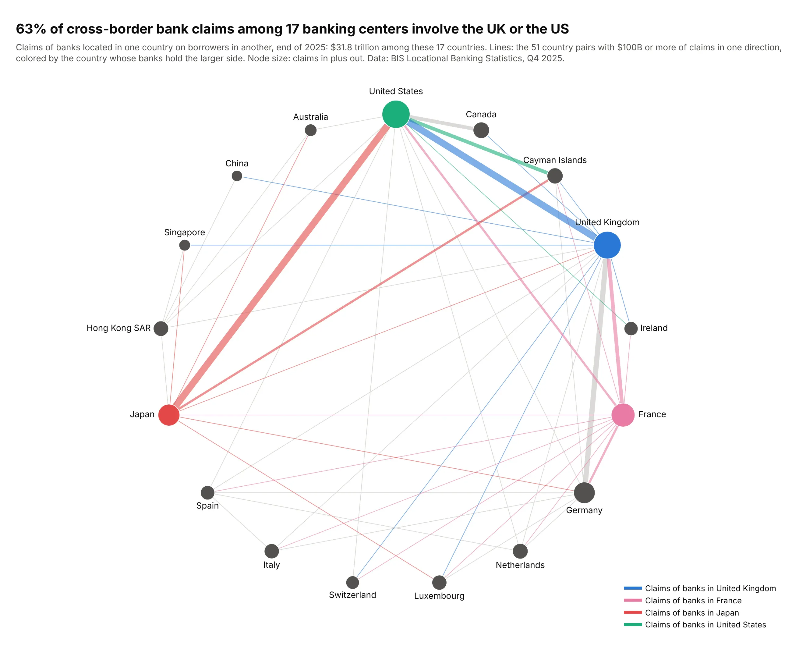
Circular network of cross-border bank claims among 17 banking centers at the end of 2025. Thick red lines run from Japan to the US and the Cayman Islands, blue from the UK to the US, gray from Germany to the UK, and pink from France

Banks located in these 17 countries held $31.8 trillion of claims on each other at the end of 2025, and 63% of it involved the UK or the US. Japan's banks held $2.3 trillion of claims on the US. Data: BIS Locational Banking Statistics.

Tip: a circular layout in a fixed order (here by region) gives every country the same room, so hubs show by their lines and not by crowding the middle.

Get the data from the BIS Locational Banking Statistics (dataset WS_LBS_D_PUB, cross-border
claims of banks in each reporting country on each counterparty country, end of 2025, US$
billions) (columns: source, target, source_name, target_name, claims_bn).

Make a plotly network graph of 17 large banking centers on a circle ordered by region.
- One edge per pair with $100B or more, colored by the lender for the UK, France, Japan
  and the US, gray otherwise; width by claims.
- Node size: claims in plus out; labels outside the circle.

4. The dollar's place in currency trading

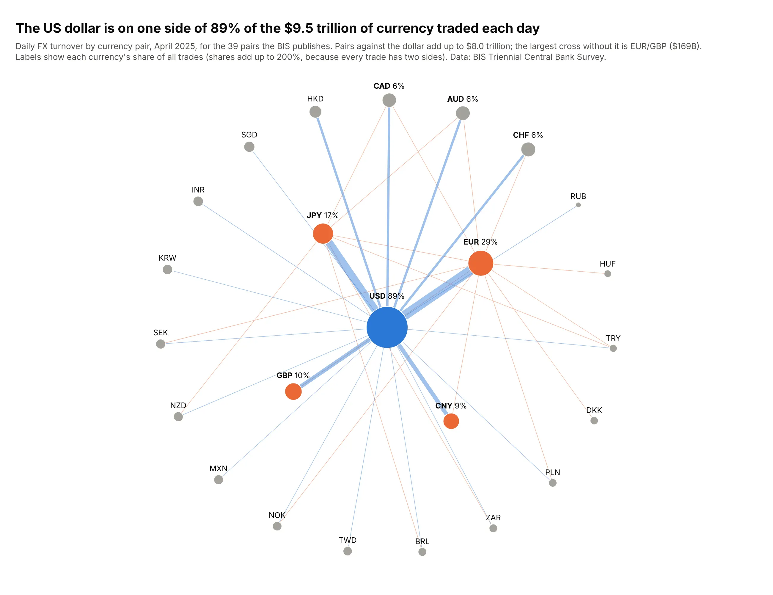
Radial network of 39 currency pairs with the US dollar in the center, the euro, yen, pound and renminbi in an inner ring and 25 other currencies outside. Thick blue lines connect the dollar to the euro and yen, and thin orange lines show the few crosses without the dollar

$9.5 trillion of currencies changed hands each day in April 2025, and the US dollar was on one side of 89% of the trades. The largest pair without the dollar, EUR/GBP, traded $169 billion a day. Data: BIS Triennial Central Bank Survey.

Tip: shell_layout with the hub alone in the first shell turns a hub-and-spoke network into a clean radial chart.

Get the data from the BIS Triennial Central Bank Survey (dataset WS_DER_OTC_TOV, FX turnover
by currency pair, net-net, April 2025, US$ billions) (columns: a, b, turnover_bn), plus each
currency's total turnover and share of trades (columns: currency, turnover_bn, share_pct).

Make a plotly network graph with nx.shell_layout: USD in the center, EUR, JPY, GBP and CNY in
the inner ring, the rest outside.
- Edge width by turnover; dollar pairs in blue, other crosses in orange.
- Node size by turnover; label each currency with its share of trades.

5. Protein interactions in lung cancer

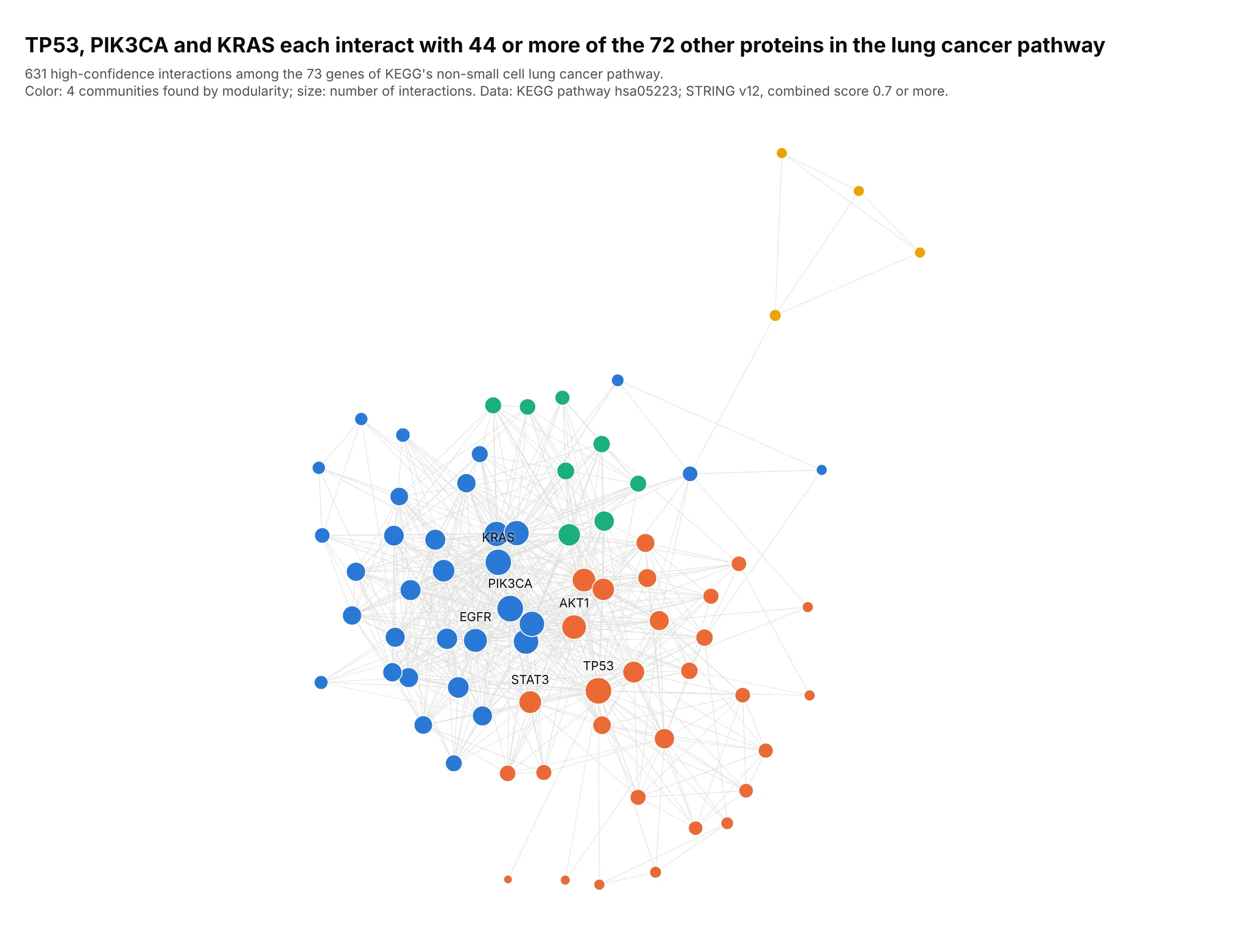
Network of the 73 genes in KEGG's non-small cell lung cancer pathway linked by 631 high-confidence STRING interactions, colored by four communities. TP53, PIK3CA and KRAS are the largest nodes, and a group of four retinoid receptors hangs off to one side

These are the 73 genes in KEGG's non-small cell lung cancer pathway, linked when STRING scores their interaction at 0.7 or more. TP53 and PIK3CA interact with 45 of the other proteins and KRAS with 44. Data: KEGG pathway hsa05223; STRING v12.

Tip: color by communities found with nx.community.greedy_modularity_communities, so the modules have names before the reader looks for them.

Get the data from KEGG (genes in pathway hsa05223, non-small cell lung cancer) and the STRING v12
API (interactions among them, Homo sapiens, combined score 0.7 or more) (columns: a, b, score).

Make a plotly network graph with networkx, Kamada-Kawai layout.
- Color nodes by greedy modularity community; size by degree.
- Thin light gray edges; label the six biggest hubs.

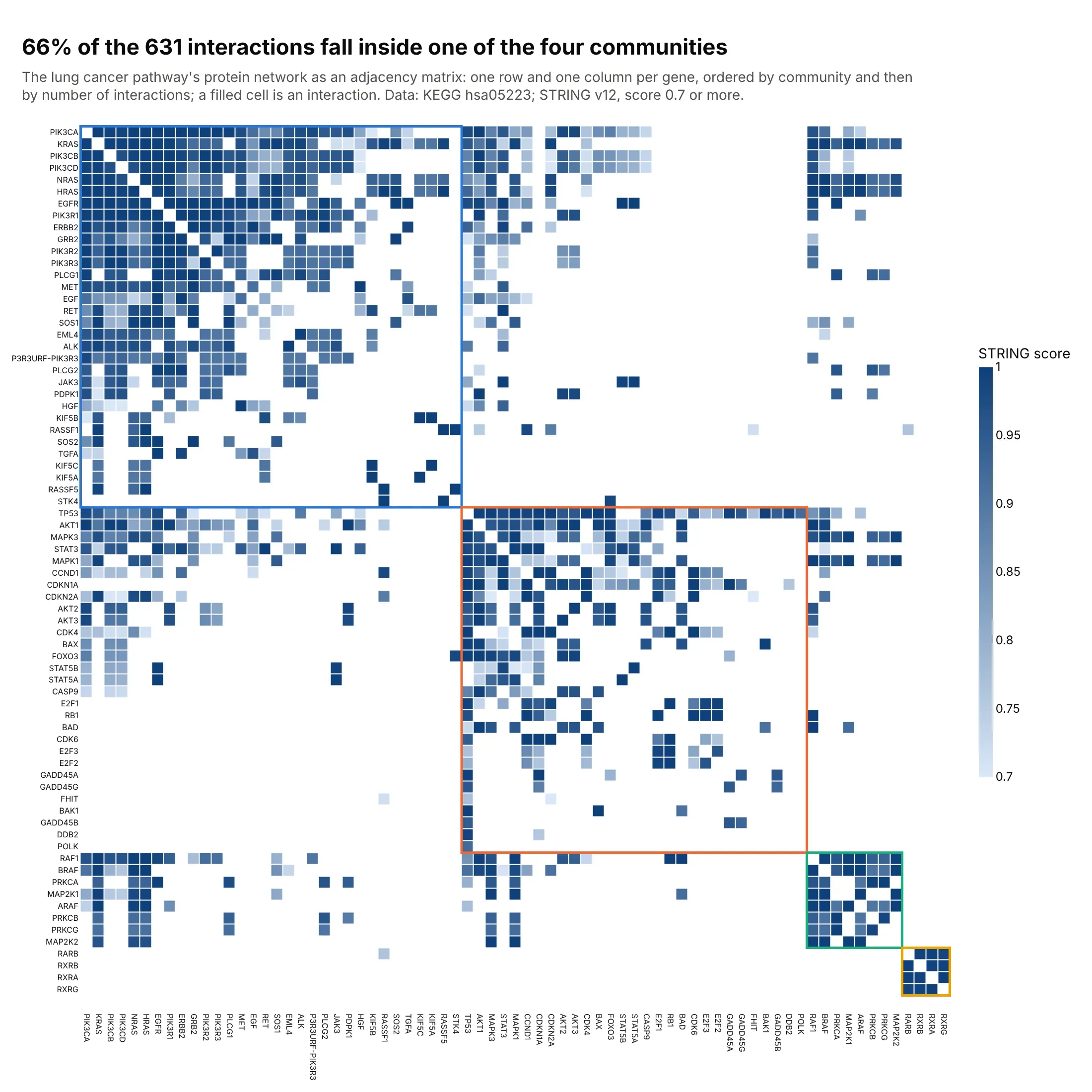
Another way to see it: with 631 links among 73 nodes, an adjacency matrix ordered by community shows that 66% of interactions fall inside one community, which the node-link view only hints at.

Adjacency matrix of the lung cancer protein network with rows and columns ordered by community: four outlined blocks on the diagonal, dense in the two large communities, and scattered cells between them

6. Drugmakers that run phase 3 trials together

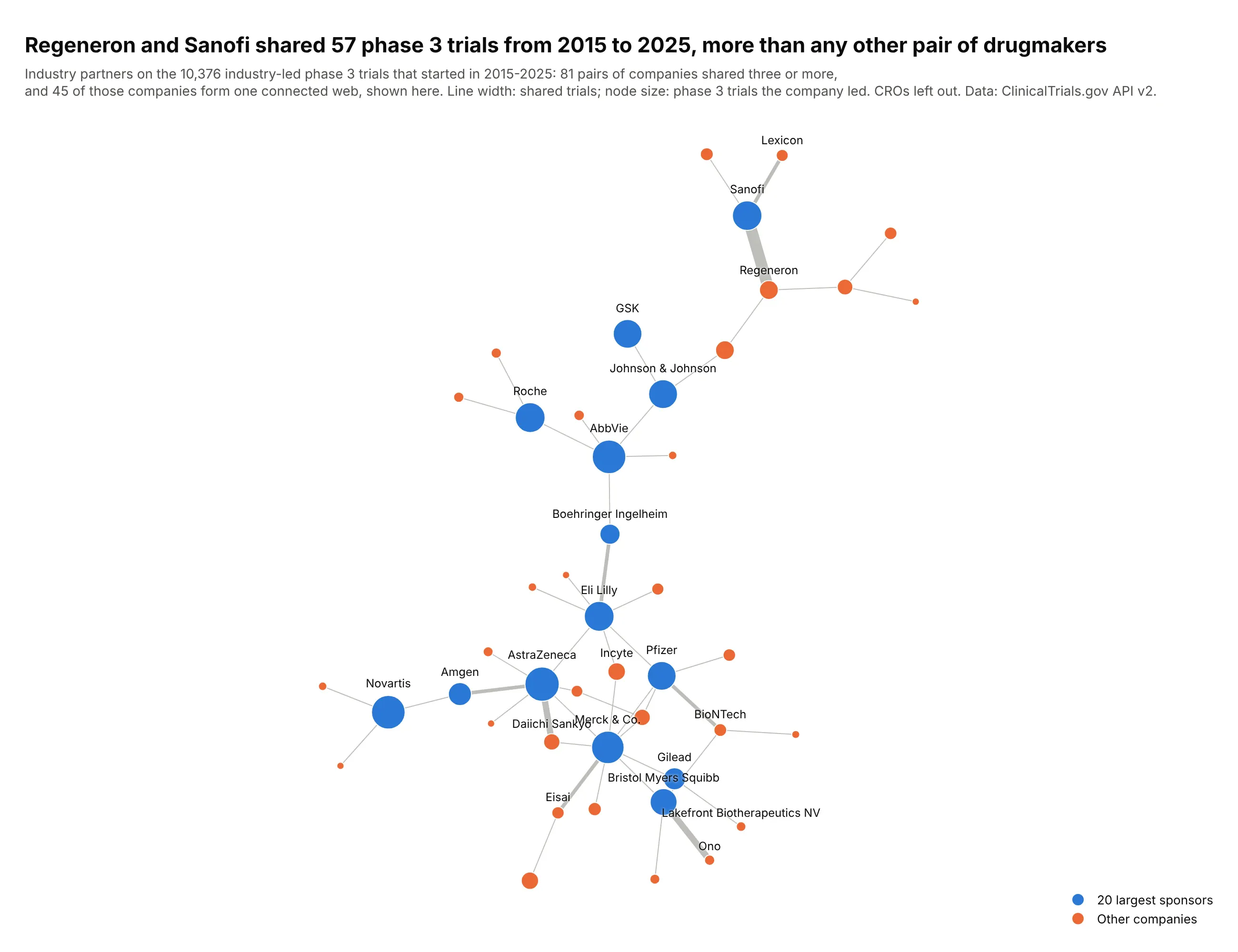
Network of 45 drugmakers linked by three or more shared phase 3 trials started 2015-2025. A thick line joins Regeneron and Sanofi; AstraZeneca, Merck, Pfizer and Eli Lilly sit at the center with many partners

Of the 10,376 industry-led phase 3 trials that started from 2015 to 2025, Regeneron and Sanofi shared 57, more than any other pair. AstraZeneca and Daiichi Sankyo (29) and Bristol Myers Squibb and Ono (26) follow. Data: ClinicalTrials.gov API v2.

Tip: keep only the largest connected component, so the chart isn't half isolated pairs.

Get the data from the ClinicalTrials.gov API v2: industry-led phase 3 studies starting
2015-2025 with their lead sponsor and industry collaborators, names normalized to parent
companies and contract research organizations removed, counted per pair of companies
(columns: a, b, trials) and trials led per company (columns: company, lead_trials).

Make a plotly network graph of pairs with 3 or more shared trials, largest connected component.
- Kamada-Kawai layout; edge width by shared trials; node size by trials led.
- The 20 largest sponsors in blue, others in orange; label them and any pair with 10+ trials.

7. A World Cup final as a passing network

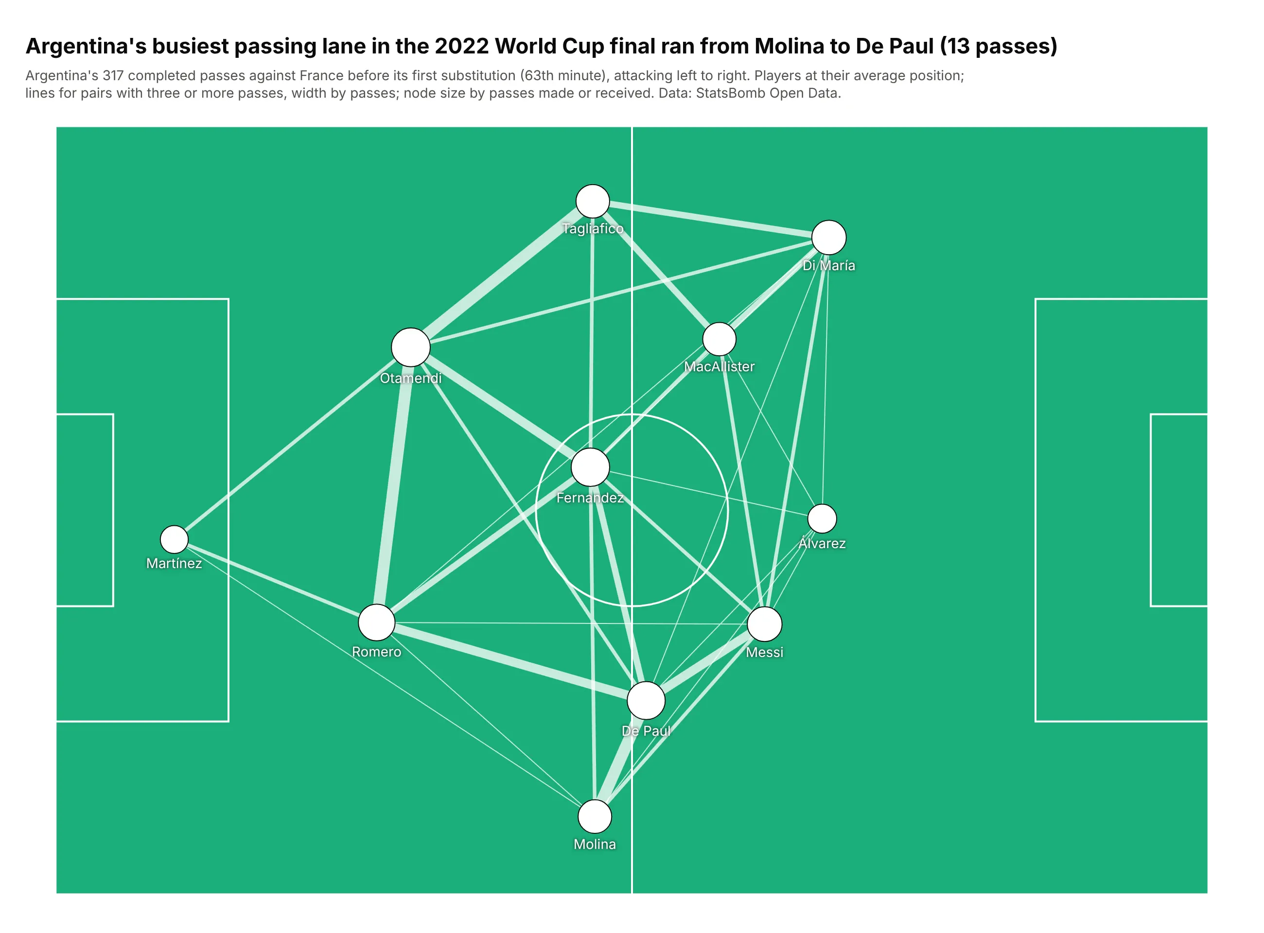
Argentina's passing network in the 2022 World Cup final before its first substitution, drawn on a green pitch with players at their average positions. The thickest lines join Molina and De Paul on the right and Otamendi, Romero and Tagliafico at the back

Argentina completed 317 passes against France before its first substitution in minute 63. Each player sits at their average position, and the busiest lane was Molina to De Paul, 13 passes down the right. Data: StatsBomb Open Data.

Tip: when positions come from the data, skip the layout algorithm and draw the context (here a pitch) with layout.shapes.

Get the data from StatsBomb Open Data (the 2022 World Cup final events, Argentina's completed
passes before its first substitution) (columns: passer, recipient, passes) and each player's
mean position on the 120 x 80 pitch (columns: player, short, x, y, touches).

Make a plotly network graph with players at (x, y) on a pitch drawn with layout.shapes.
- Edges for pairs with 3 or more passes in both directions together, white, width by passes.
- White nodes sized by touches, short names below; y axis reversed.

8. Kinase inhibitors and the kinases they act on

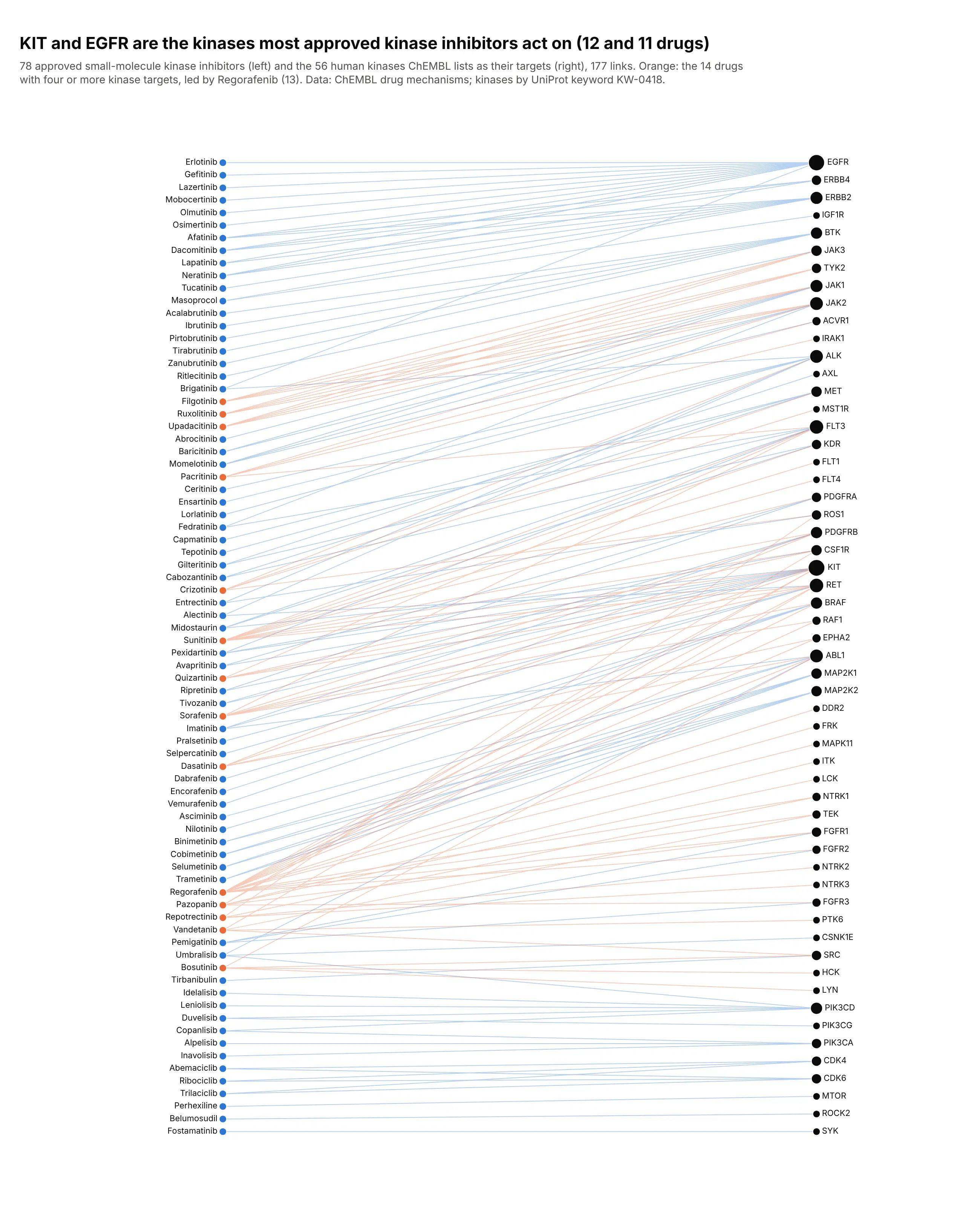
Two-column network of 78 approved kinase inhibitor drugs on the left and the 56 kinases they act on on the right. EGFR, JAK, BTK, CDK4/6 and PI3K drugs form flat bundles, and multi-target drugs such as regorafenib, sunitinib and pazopanib fan out in orange

Of 78 approved kinase inhibitor drugs, 12 act on KIT and 11 on EGFR, and 14 drugs act on four or more kinases. A bipartite layout puts the drugs on one side and their targets on the other, so both the busiest targets and the drugs that hit many targets stand out. Data: ChEMBL drug mechanisms (approved small molecules), UniProt kinase keyword.

Tip: order both columns by the barycenter method (each node at the mean position of its neighbors, repeated a few times) to cut line crossings.

Get the data from the ChEMBL web services (ebi.ac.uk/chembl/api/data/mechanism.json, max_phase=4,
action_type=INHIBITOR, approved small molecules acting on one human protein) and keep targets with
UniProt's Kinase keyword (KW-0418)
and shape it into a table
(columns: drug, kinase).

Make a plotly network graph with nx.bipartite_layout: drugs on the left, kinases on the right.
- Order both columns by the barycenter method to cut crossings; label every node.
- Drugs acting on four or more kinases, and their links, in orange; the rest in blue.
- Kinase node size by number of drugs; title with the two most targeted kinases.