
Chris Parmer
November 15, 2026
Cohort Retention Heatmaps - A Complete Guide
TL;DR
- A cohort retention heatmap groups customers by the month of their first purchase (their cohort), draws one row per cohort and one column per month counted from that first month, and colors each cell by the share of that row's original customers who bought in that month, so the table fills in as a triangle.
- Cohort retention heatmaps are also known as cohort analysis charts and retention tables. Google Analytics 4 calls them a cohort exploration, Amplitude a retention analysis, and actuaries use the same shape as a development triangle. They are similar to heatmaps, line charts (retention curves) and area charts (layer cake charts).
- Month 0 is the month of the first purchase and month 2 is the second calendar month after it. The cells are percentages, not head counts: in the retail example, 33% of the December 2009 cohort, 319 of its 955 customers, bought in month 2 (February 2010).
- Read across a row to judge one cohort, down a column to compare cohorts at the same stage (for example after a change to onboarding), and along a diagonal to see one calendar month, such as November 2010, when every 2010 cohort was busy, and December 2010, when every one was quiet.
- The same data gives several tables that answer different questions: who bought in month N, who had come back by month N (cumulative retention), who bought in month N or later (unbounded retention), head counts and revenue. You can make all of them with Plotly in Python from pandas groupby and go.Heatmap.
What is a cohort retention heatmap?
Cohort retention heatmaps look like this:
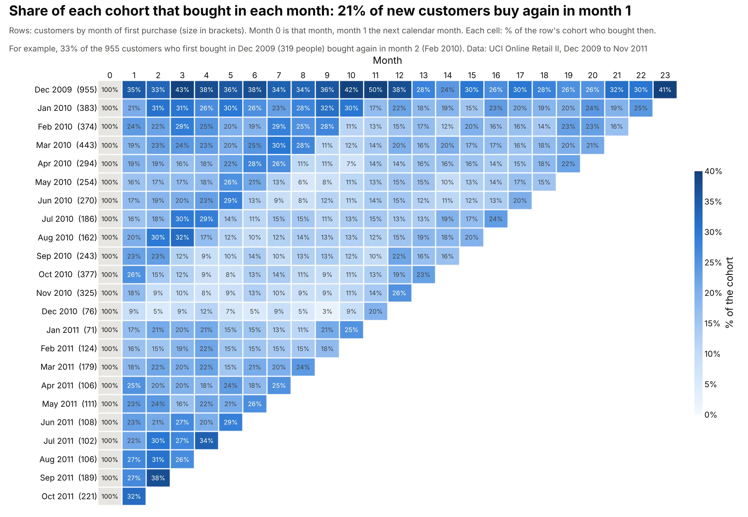
Data: UCI Online Retail II, the invoices of a UK online giftware retailer from December 2009 to November 2011, from the University of California, Irvine (UCI) Machine Learning Repository. 5,850 customers with a customer ID.
How do you read a cohort retention heatmap? In the example above, notice these things:
- Each row is a cohort, the customers whose first purchase was in that month, with its size in brackets. The grey month 0 column is that first month, where the whole cohort (100%) bought. The January 2010 cohort has 383 customers, and 21% of them (79 customers) bought again in month 1, February 2010.
- Each column is a month number counted from each row's own first month, so a column compares cohorts at the same stage. Across the cohorts from January 2010 to October 2011, 21% of new customers bought again in month 1.
- The top row is much darker, at 33% to 50% in months 1 to 12, because the data start in December 2009. That cohort holds every customer who bought that month, including long-standing ones, so it measures regulars and not new customers.
- The 2010 rows turn pale at the same moment, December 2010, which sits further left in each newer row, and the 2011 cohorts start stronger: their month 1 averages 23%, against 19% for the 2010 cohorts.
- Blank cells are months after the end of the data, which is what gives the table its triangle shape.
It's often used for charts like these:
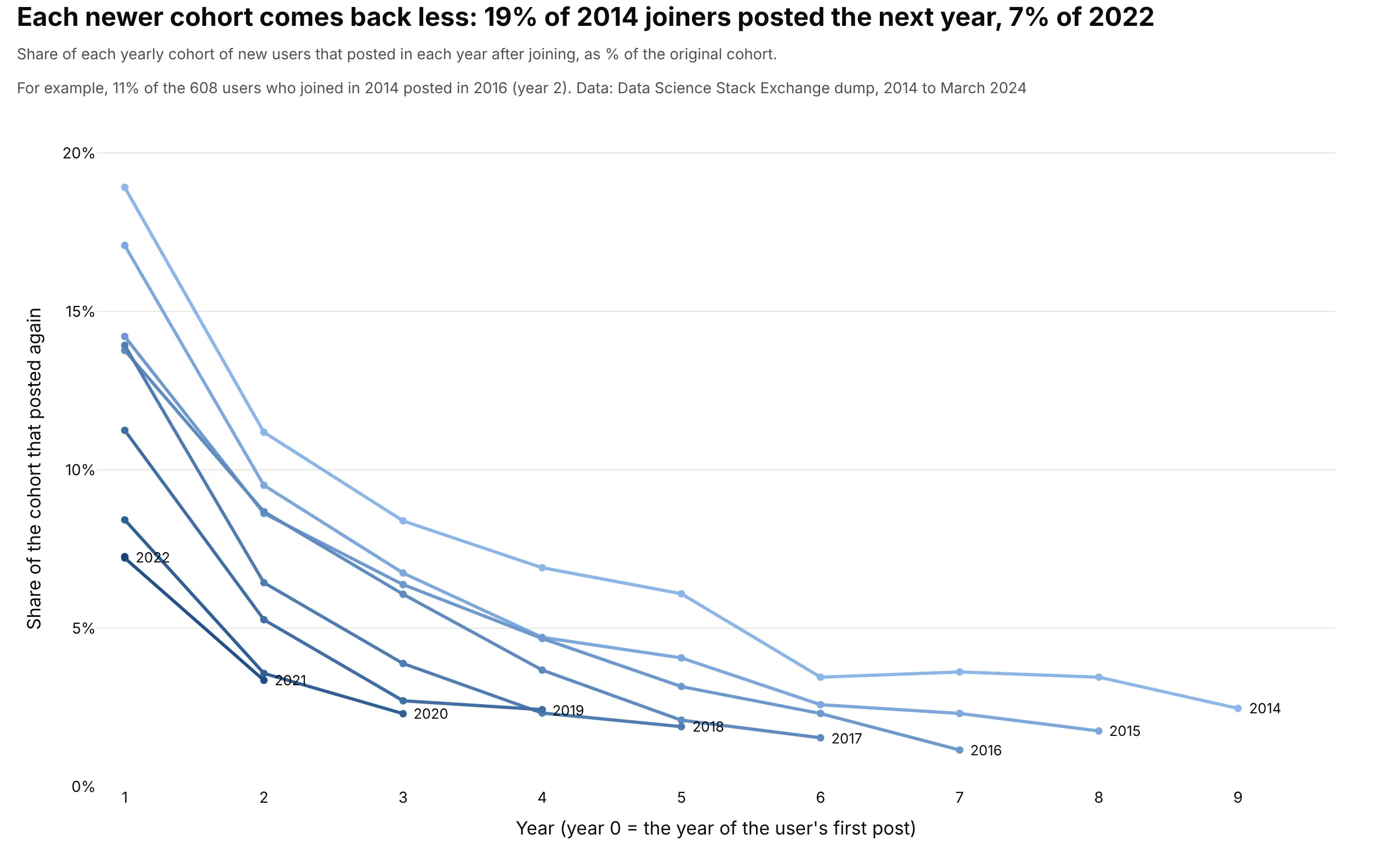
Retention curves. One line per cohort puts the cohorts on the same axes, so a newer cohort that retains less is a line below the older ones: 19% of the 608 users who joined Data Science Stack Exchange in 2014 posted again the next year, and 7% of the 2,466 who joined in 2022. Data: Stack Exchange data dump for datascience.stackexchange.com on the Internet Archive (CC BY-SA 4.0), questions and answers by users with an account.
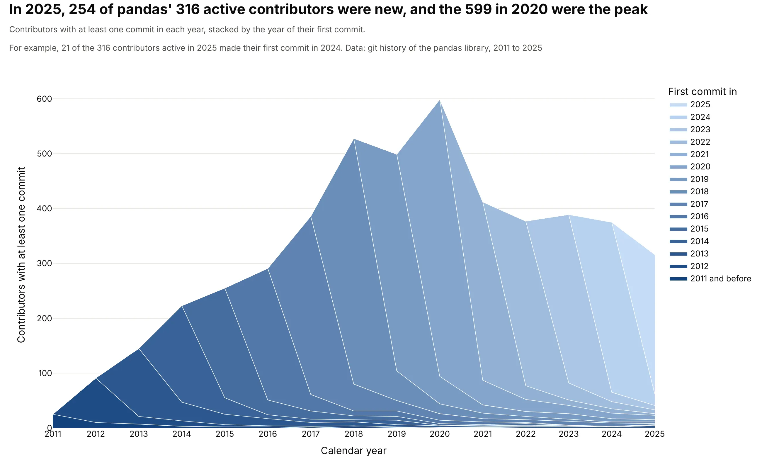
Layer cake charts. A stacked area chart of how many people are active each year, one layer per cohort, shows how much of today's activity comes from newcomers: 254 of the 316 people who committed to the pandas library in 2025 made their first commit that year. Data: the git history of the pandas library on GitHub, authors identified by commit email address.
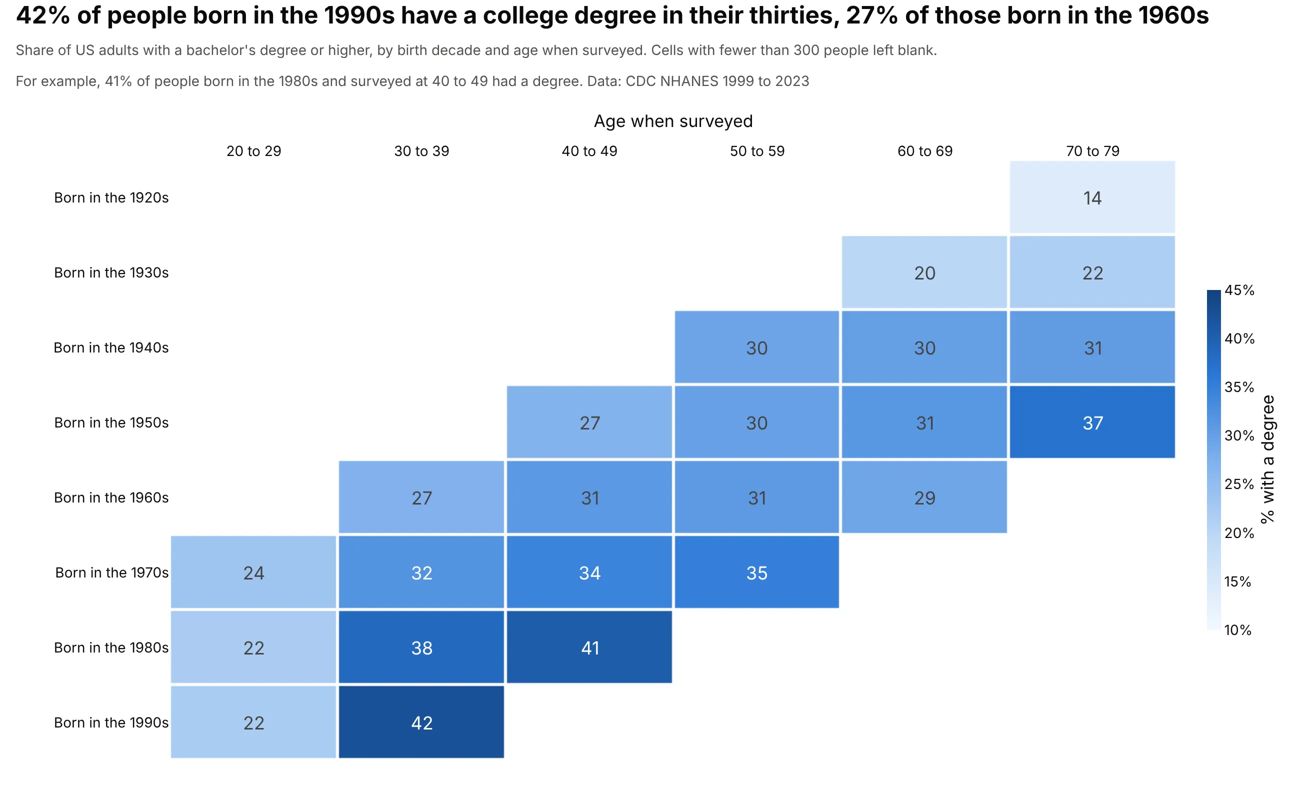
Generations in a survey. The same layout with birth decades as cohorts and age bands as columns shows that 42% of people born in the 1990s have a college degree in their thirties, against 27% of those born in the 1960s. Here each cell is the share of the people surveyed at that age, not of one group followed over time. Data: US Centers for Disease Control and Prevention (CDC), National Health and Nutrition Examination Survey (NHANES), 1999 to 2023, 58,013 adults aged 20 to 79.
What "month 2" means, and how the table is calculated
A cohort table needs one record per customer and period, such as "customer 12,583 bought something in March 2010". Three steps turn those records into the heatmap:
- Assign each customer to a cohort by the calendar month of their first purchase. That month is the cohort's month 0. A customer whose first purchase was in January 2010 belongs to the January 2010 cohort for good, however often they buy later.
- Number the later months by counting calendar months from month 0. Month 1 is the next calendar month and month 2 the one after, so for the December 2009 cohort month 2 is February 2010, and for the January 2010 cohort it is March 2010. The code in this guide subtracts the two calendar months and ignores the day, so a customer who first bought on December 31, 2009 and again on January 2, 2010 counts in month 1 although only two days passed, and a second order later in the first month counts for nothing, because it is still month 0. Mixpanel's retention report calls this calendar interval retention. Its other option, rolling interval retention, counts from the exact time of the first event instead, so month 1 there is 30 to 60 days after it. The retail data here has one row per customer and month, so calendar months are the only choice for it, and whichever you use should go in the subtitle.
- Count the distinct customers in each cohort and month, and divide by the cohort's size, which is the count in month 0. Every cell is a share of that row's original cohort, never of the customers who were still active the month before, so a customer who skips month 1 and buys in month 2 counts in month 2, and a row can go up from one month to the next.
Here's the top-left corner of the table with all three numbers in each cell: the share, the head count behind it and the calendar month it falls in.
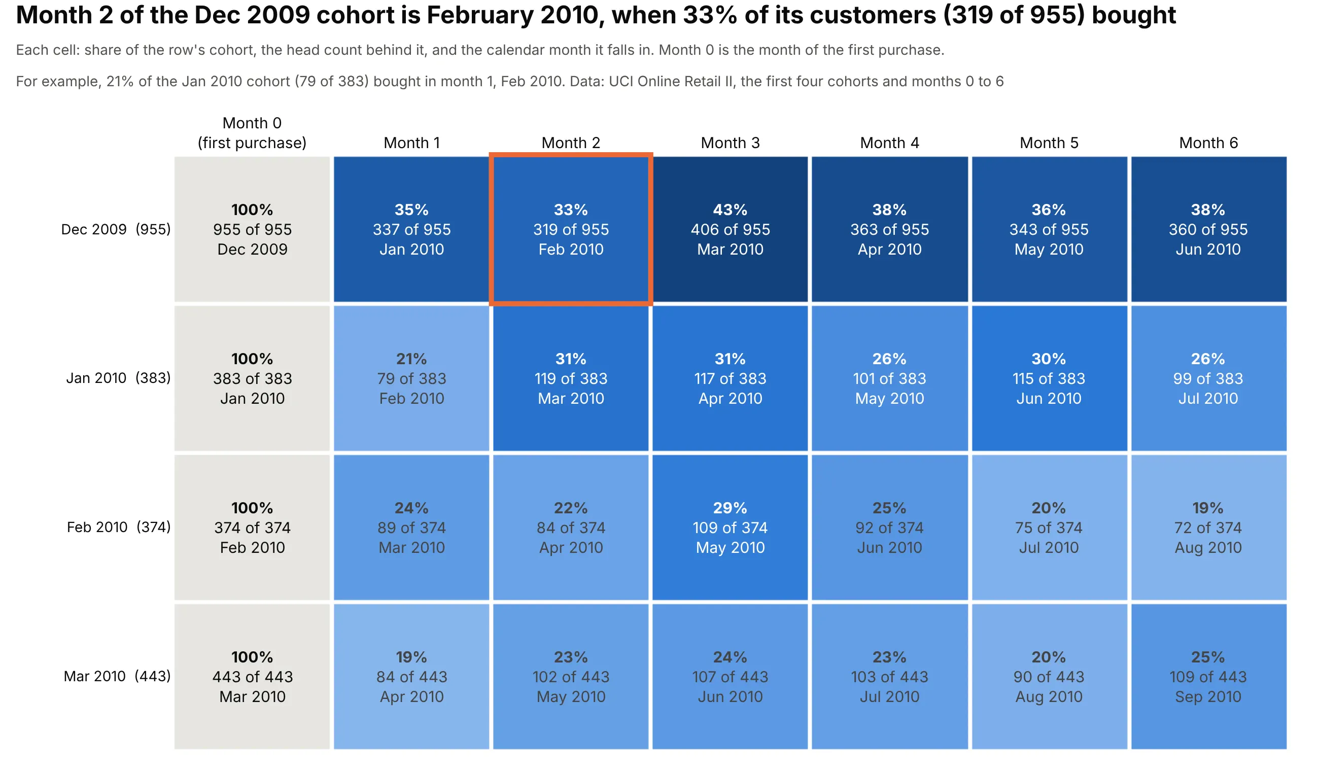
So the 33 and the 43 in the top row of the main chart are percentages: 33% of the 955 customers in the December 2009 cohort (319 people) bought in month 2, February 2010, and 43% (406 people) bought in month 3, March 2010.
Month
Calendar month
Customers who bought
Share of the 955 in the cohort
0
December 2009
955
100%
1
January 2010
337
35%
2
February 2010
319
33%
3
March 2010
406
43%
4
April 2010
363
38%
5
May 2010
343
36%
6
June 2010
360
38%
The December 2009 row is the first cohort of the data, so it contains everyone who bought that month, including customers who had been buying for years before the data begin. That is why it sits at 33% to 50%, against 3% to 38% for the later cohorts in months 1 to 12. The January 2010 row is a cleaner example of new customers: 79 of 383 (21%) bought in month 1, 119 (31%) in month 2 and 117 (31%) in month 3.
The same table in head counts
Printing the number of customers instead of the share lets readers check any percentage by hand, and shows how much business each cohort brings in:
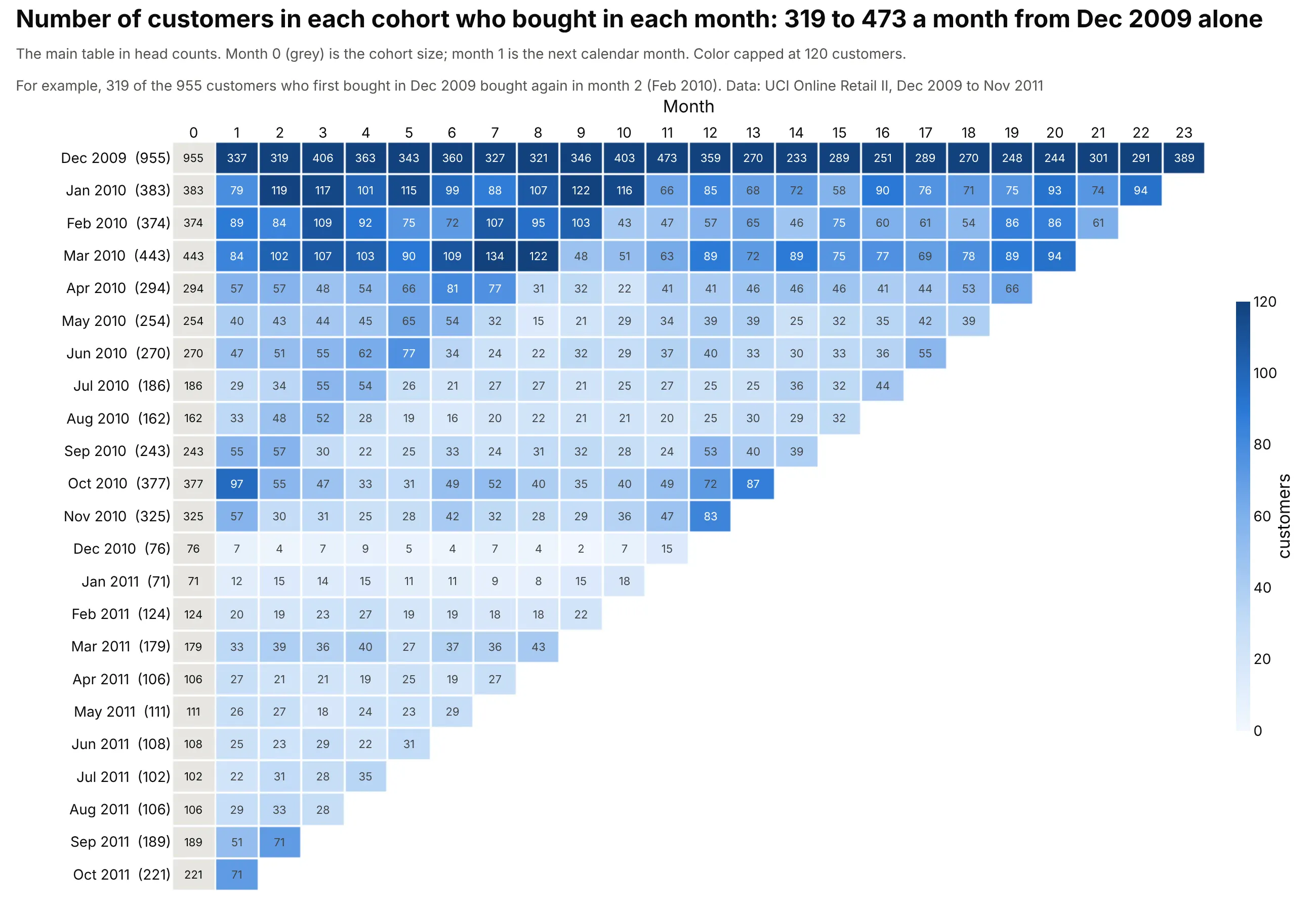
The color in a head-count table compares cohorts by size, not by loyalty. The December 2009 cohort alone has 319 to 473 buyers a month in its first year, while the December 2010 cohort of 76 never has more than 15, so the top row is dark and the rest pale. Use the counts to check the percentages and to judge how noisy a row is (one customer is 1.3% of the December 2010 cohort), and use the percentages to compare cohorts.
Two more details decide whether the table can be trusted. First, a month that hasn't happened yet is blank, not 0%. The data end on December 9, 2011, so December 2011 was dropped, and the November 2011 cohort of 191 customers has no row because it has no month 1 yet. Second, the first cohort of any data set is suspect for the reason above, so mark it or start the table with the second cohort.
How to read a cohort retention heatmap
The same table answers three different questions depending on the direction you read it: a row follows one group of customers, a column compares groups at the same stage, and a diagonal is one calendar month. Every percentage in these charts is a share of that row's own original cohort, and one color scale covers the whole table, so equal colors mean equal shares in every row. (Mixpanel's heat map instead shades each cohort row relative to itself, which shows a row's shape but makes rows hard to compare.)
Across a row: was this cohort good?
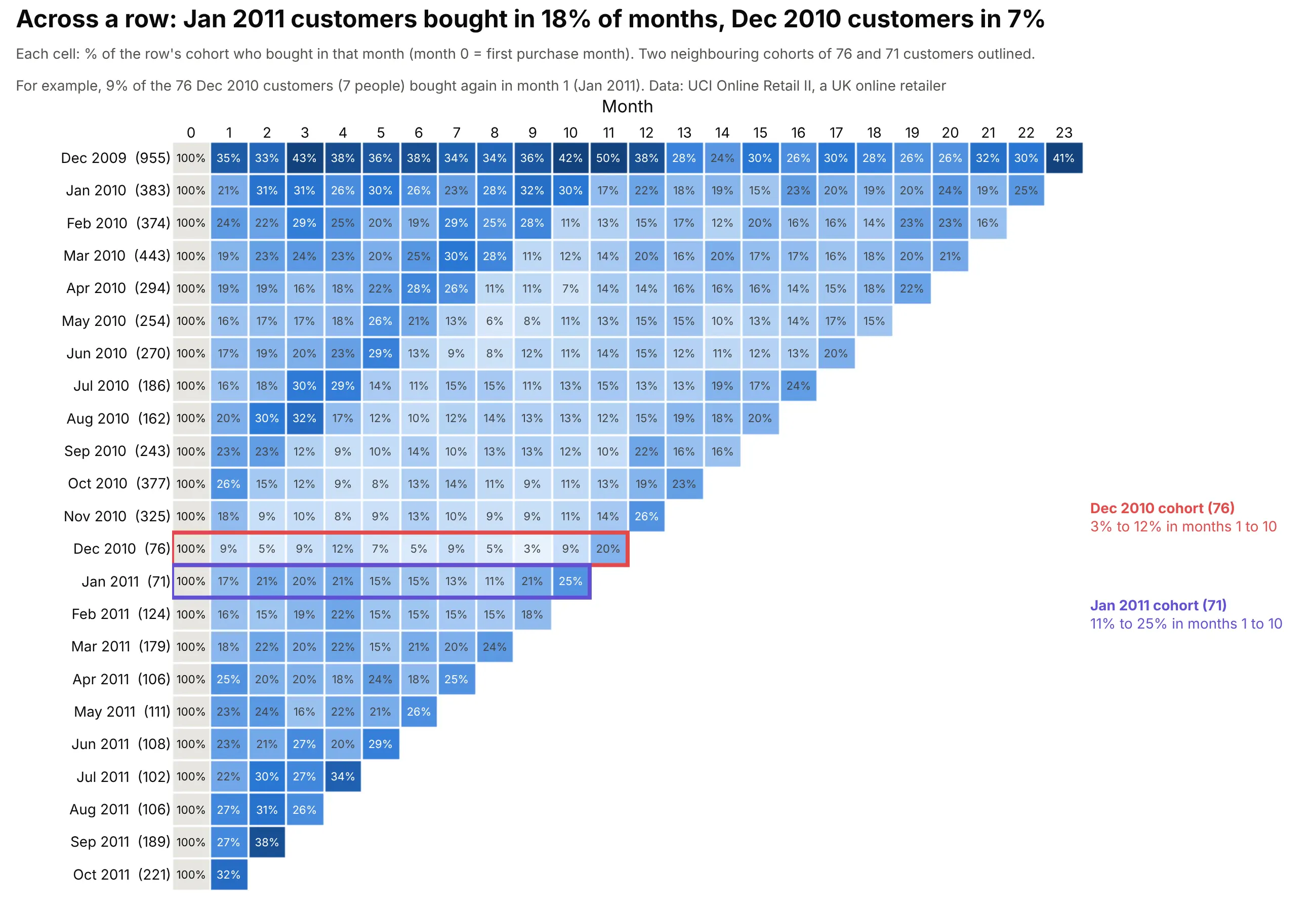
A row follows one cohort from its first month, so it tells you whether those customers were worth winning. On average 7% of the December 2010 cohort (76 customers) bought in each of months 1 to 10, and never more than 12% in any one of them. The January 2011 cohort, almost the same size at 71 customers, averaged 18% over the same months. A difference in how or when customers arrived shows up as a whole row that is paler or darker than its neighbours. A plausible reason is that a December first purchase is more often a one-off Christmas order, but the data can't confirm that. Small cohorts like these two are noisy, since one customer is more than 1% of the row, so a single weak row is a question to ask, not a conclusion.
Down a column: are cohorts at the same stage getting better?
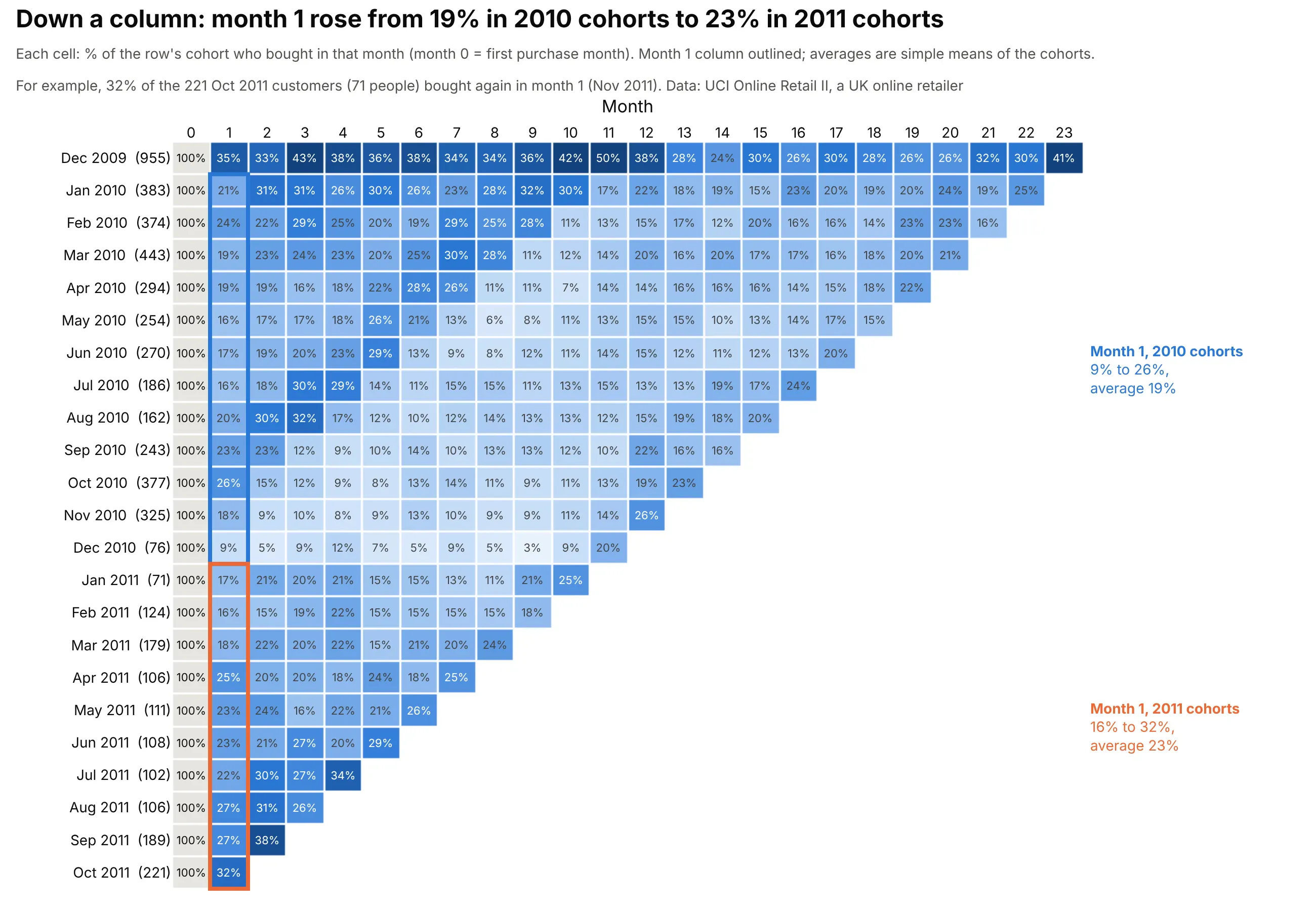
A column holds every cohort at the same stage of its life as customers, so it is where you look for the effect of anything tied to a customer's age: an onboarding sequence, the end of a free trial, or a reminder email. Here's a hypothetical example, since we don't know what this retailer did. Suppose it started emailing every customer in their third month from January 2011 onward. The October 2010 cohort was the first to reach month 3 after that (its month 3 is January 2011), so the month 3 column would darken from the October 2010 row down, while months 2 and 4 stayed as they were and the older rows, whose month 3 had already passed, stayed pale. A change shaped like a column is a sign that something tied to the customer's age is working, and it lets you track long-term engagement cohort by cohort.
In the real data, the month 1 column does change. It runs from 9% to 26% for the 2010 cohorts (19% on average) and from 16% to 32% for the January to October 2011 cohorts (23% on average). Before crediting anything the retailer did, check the calendar, because every cell in a column falls in a different calendar month. Customers won earlier were buying less in 2011: in each month from January to October 2011, 12% to 19% of the customers who had first bought between January 2010 and the month before bought again, against 19% to 28% from February to November 2010. So the calendar was working against the 2011 cohorts, and the rise in month 1 is not a seasonal effect.
Along a diagonal: what happened in one calendar month?
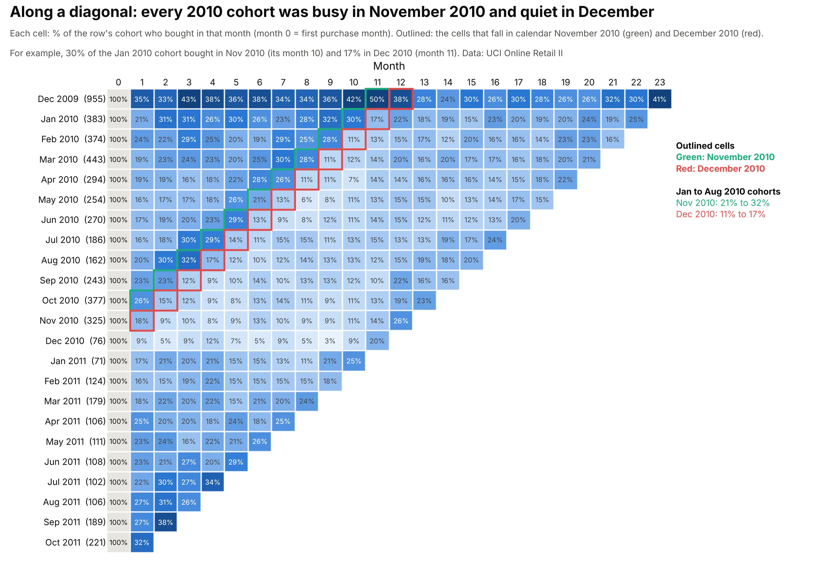
A cohort's month 0 plus the month number gives the calendar month, so all the cells that fall in one calendar month lie on a diagonal, one column to the left for each newer row. When the same diagonal is darker or paler in many rows at once, the cause is the calendar (a holiday, a price change, an outage, a campaign) and not any one cohort. In the retail data the green diagonal, November 2010, holds 21% to 32% for the January to August 2010 cohorts, and the red diagonal right next to it, December 2010, holds 11% to 17% for the same cohorts. The pale band under it continues into 2011. Counting, for each calendar month, the customers whose first purchase was between January 2010 and the month before, 27% bought in November 2010, 14% in December 2010 and 12% in January 2011. The next November lifts again, to 23% in November 2011 against 19% in October 2011. UCI's description of the data says that many of the company's customers are wholesalers, which fits buying for Christmas in the autumn, though the data can't say why.
Plotly can also draw the table with calendar months on the x axis instead of month numbers, which turns a diagonal into a vertical stripe (see example 3 below).
Retention in month N, by month N, or in month N or later
The main table counts a customer in a month only if they bought in that month. That's the right question for a shop that expects a purchase every month, but many products are used every few months at irregular intervals, and then "did they buy in month 4?" says little about whether you've lost them. The same orders give two other tables for that, plus revenue in place of customers, and each answers a different question.
Question
Table
A customer counts in month N if they
How many bought in month N?
In month N (the main table)
bought in month N
How many have come back at least once by month N?
Cumulative retention
bought in any month from 1 to N
How many have not been lost by month N?
Month N or later (unbounded retention)
bought in month N or any later month
How much money does the cohort still bring in?
Revenue retention
(revenue in month N divided by revenue in month 0)
Amplitude's retention documentation calls the first "Return On" (formerly N-day retention) and the third "Return On or After" (formerly unbounded retention), and Mixpanel calls them "On" and "On or After". Whichever you draw, say in the title and subtitle what a cell counts.
Bought again by month N (cumulative retention)
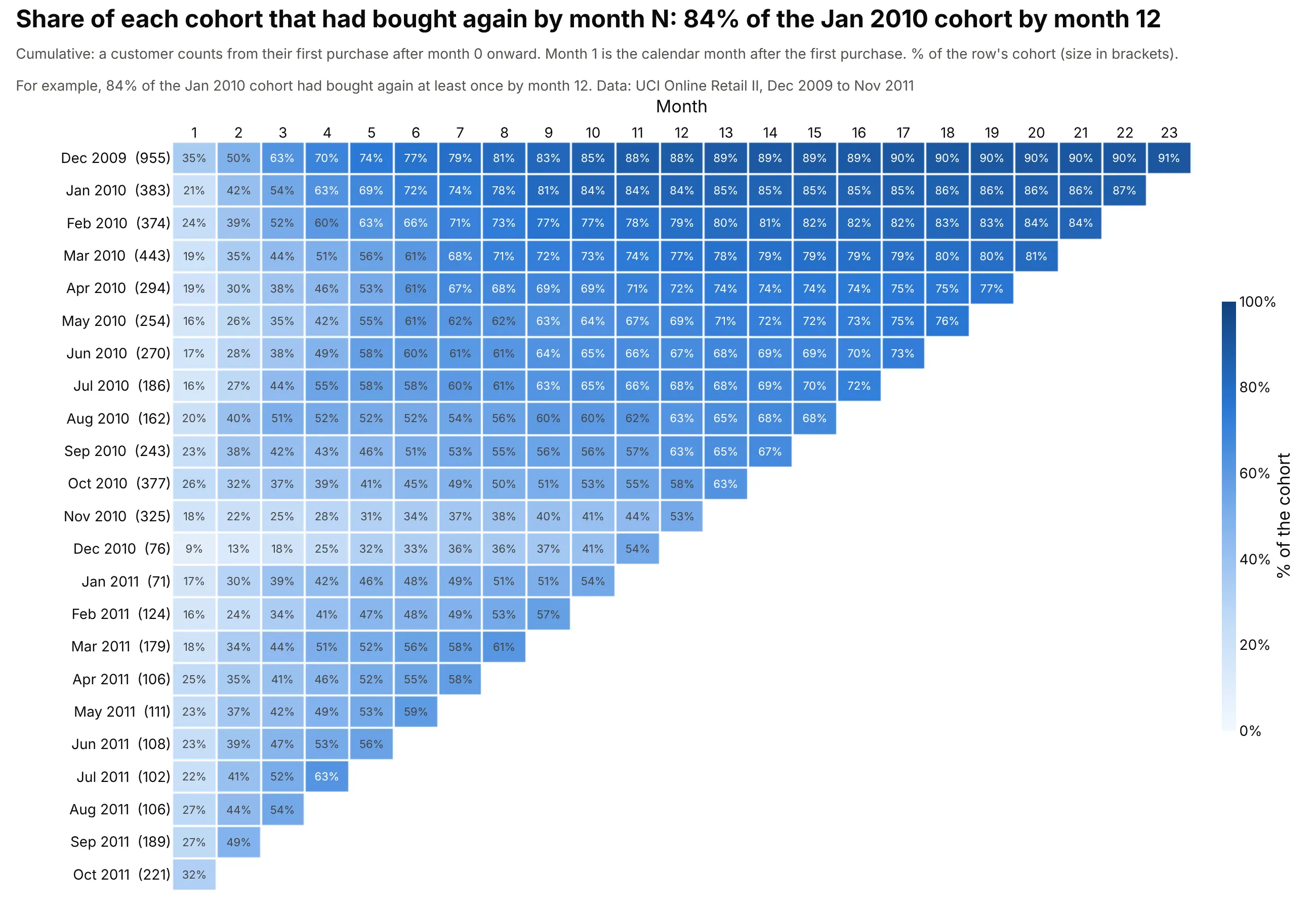
Each cell is the share of the cohort that had bought again at least once in months 1 to N, so every row only rises. It answers "how many customers have come back yet?": 21% of the January 2010 cohort had bought again by month 1, 54% by month 3, 72% by month 6 and 84% by month 12. The newer 2010 cohorts reach less: by month 12, the share falls from 84% for January 2010 to 53% for November 2010. Cumulative retention works like a Kaplan-Meier curve for the time until the second purchase. It never goes down, so it hides customers who came back once and then left.
Bought in month N or later (unbounded retention)
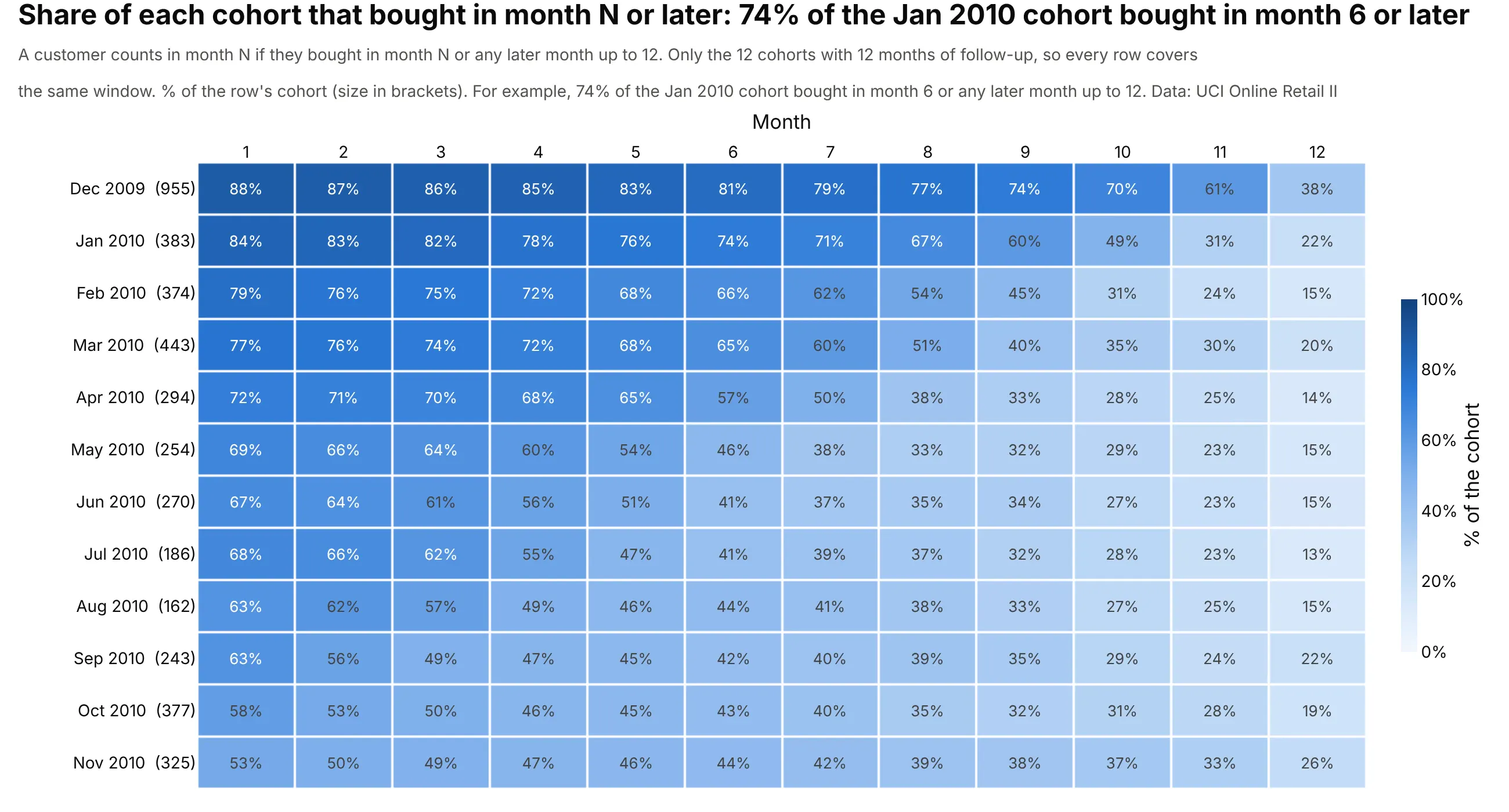
This one is the opposite of cumulative retention. A customer counts in month N if they bought in month N or in any month after it, so a cell is the share of the cohort that you hadn't yet lost by month N. It's the right table when customers come back every few months at random, because a customer who skips months 4 and 5 and buys in month 6 still counts in month 4. For the January 2010 cohort only 26% bought in month 6 itself, but 74% bought in month 6 or later.
"Or later" needs care, because newer cohorts have less of a future in the data. Counted up to the end of the data, 87% of the January 2010 cohort bought in month 1 or later, against 32% of the October 2011 cohort, but the October 2011 cohort had only one month to do it in. That bias is called right-censoring, and it makes every newer cohort look worse. The chart above fixes it by counting only months 1 to 12 and showing only the 12 cohorts, December 2009 to November 2010, that have all 12 months in the data, so every row covers the same window. The month 1 column of this table equals the month 12 column of the cumulative table (84% for January 2010 in both), because "bought in month 1 or later, up to month 12" and "came back by month 12" are the same customers. Even with a fair window the newer cohorts fall behind: 53% of the November 2010 cohort bought in month 1 or later, against 84% of January 2010, partly because the November cohort's window is the quiet year 2011.
Revenue retention instead of customer retention
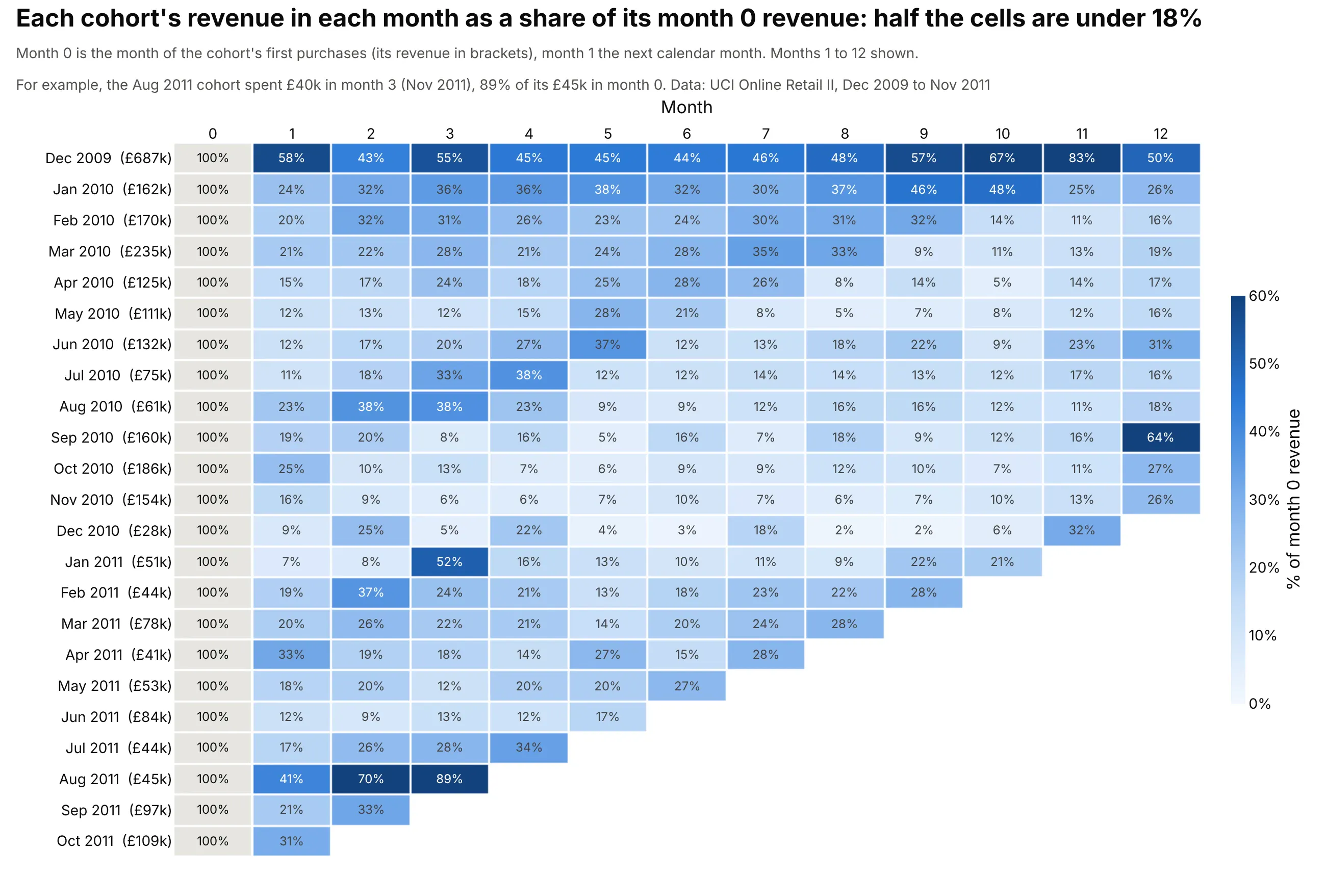
Dividing each month's revenue by the cohort's month 0 revenue shows how much money the cohort still brings in, and it can pass 100% when customers who stay spend more. In this data about half the cells are under 18%. The December 2009 cohort reached 83% in month 11, and the August 2011 cohort (£45,000 in its first month) 89% in month 3. Data: UCI Online Retail II, revenue as quantity times unit price, per cohort and month.
Tip: write the cohort's first-month revenue in the row label, so readers can see that the 89% sits on a small base.
The retention curves at the top of this guide are the fifth variant: the same rows drawn as lines, which suits comparing a few cohorts more than scanning many.
A short history
The word cohort for a group followed through time comes from demography. In 1965 the sociologist Norman Ryder argued in The Cohort as a Concept in the Study of Social Change (American Sociological Review) that people born in the same period should be analyzed together, and demographers draw them on a Lexis diagram, named after Wilhelm Lexis, where calendar time runs across, age runs up and each birth cohort is a diagonal band. Insurers lay out claims in a development triangle in the chain-ladder method, which has the same shape as a retention table.
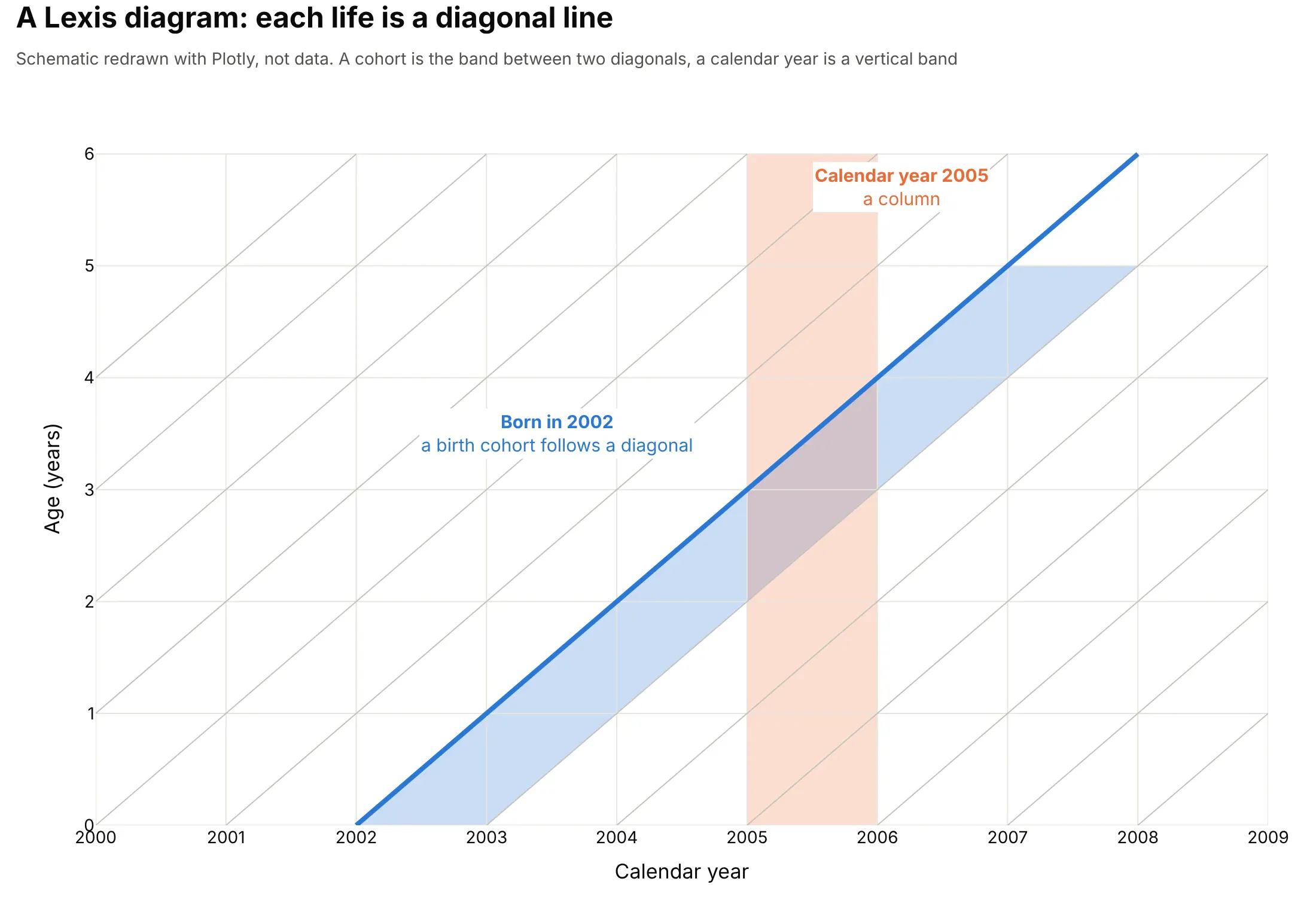
A Lexis diagram, redrawn as a schematic (not data).
Business uses came with web start-ups. Fred Wilson, a venture investor, wrote about the cohort analysis on October 6, 2009, after Dave McClure's Startup Metrics talk, with cohort charts of new Twitter users. Andreessen Horowitz's list of 16 startup metrics names retention by cohort as the engagement measure investors want to see, and Wikipedia's cohort analysis article, which separates the business practice from the cohort study in medicine, cites the book Lean Analytics (2013) among its sources. The layer cake chart came from the same world: Custora's layer cake graph, as quoted by R-bloggers in 2014, shows revenue or profit by cohort in calendar time.
Alternatives to a cohort retention heatmap
Here's the same customer data drawn six ways. Some are better for the question, some worse, some just different:
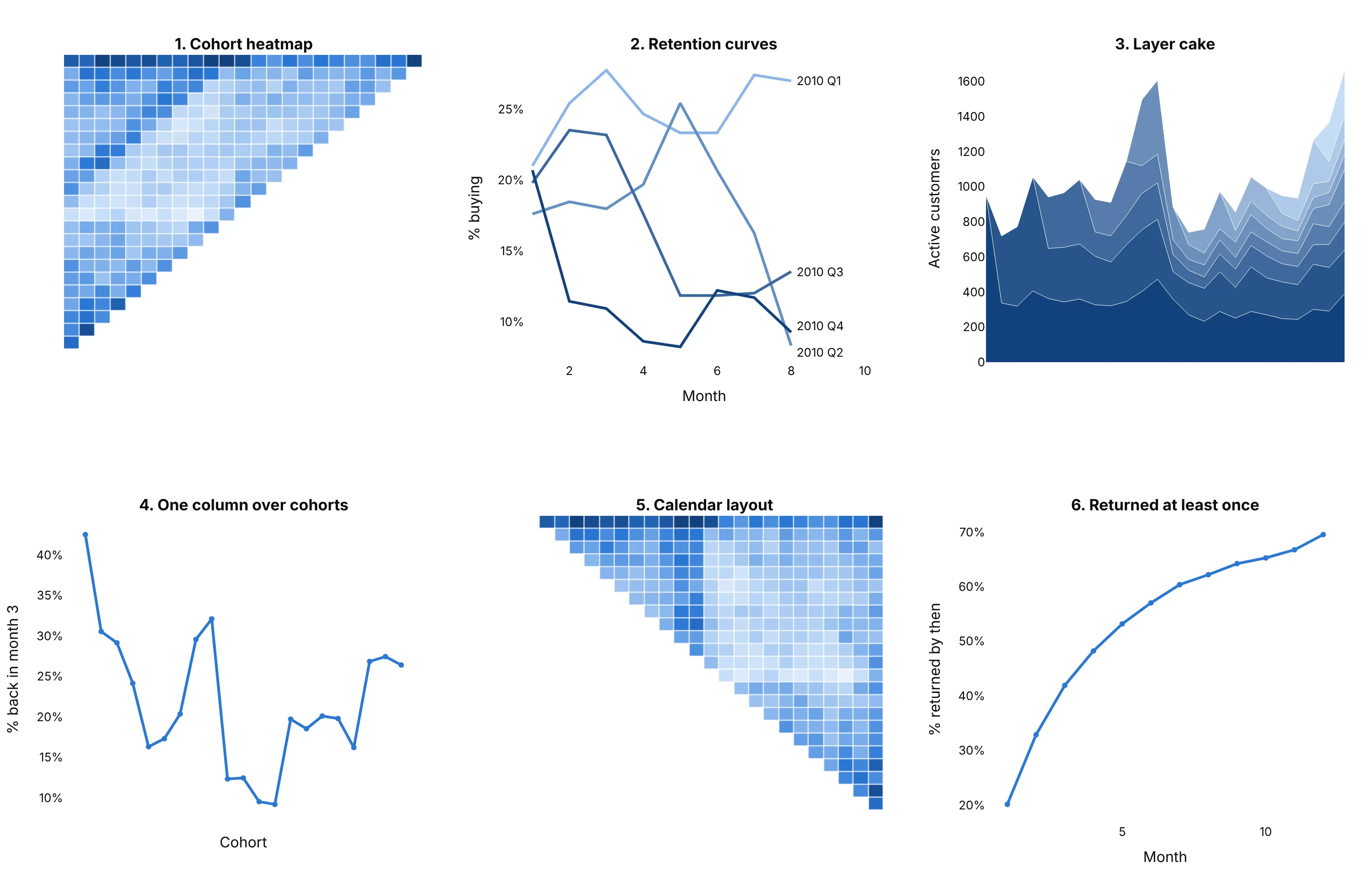
- Cohort heatmap (best for scanning every cohort and month at once). It shows decay, cohort quality and calendar effects in one table, and with numbers in the cells it doubles as the data.
- Retention curves (works too, for a few cohorts). Lines put cohorts on a shared axis and make differences easy to measure, but more than about eight lines tangle, so quarterly or yearly cohorts suit them better than monthly ones.
- Layer cake chart (different). It stacks how many customers, or how much revenue, each cohort contributes in each calendar month, so it answers how much of this month's business is new. It cannot show retention rates, because layers of different sizes are hard to compare.
- One column over cohorts (better for a trend). A line of month 3 retention by cohort, from 43% to 9% to about 27% in the retail data, is the clearest way to show whether newer cohorts are better, at the cost of the rest of the table. See line charts.
- Calendar layout (different). The same cells with calendar months as columns, which makes seasonal effects stripes (see example 3).
- Share who have returned at least once (different). The cumulative retention of all the January to November 2010 customers pooled, which only rises and reaches about 70% by month 12. It summarizes the cumulative table in one line but hides the differences between cohorts.
How to make a cohort retention heatmap
With AI
ChatGPT, Claude Code, GitHub Copilot, Cursor and other AI tools are excellent at writing Plotly code. Name Plotly in the prompt, and say how a customer is assigned to a cohort, how months are numbered and what counts as retained:
Make a plotly cohort retention heatmap from orders.csv (columns: customer, date).- A customer's cohort is the calendar month of their first order (month 0); month 1 is the next calendar month.- Cell value: the share of the cohort's original customers who ordered in that month, as a percentage of thecohort size, with a % sign in every cell.- Show month 0 as a grey 100% column outside the color scale. Months after the end of the data are blank, not 0%.- One color scale for the whole table, from white to blue, capped at 40% so ordinary cells stay readable.- Row labels "Jan 2010 (383)" with the cohort size, and "Month" as the column title.- A title that says what a cell is ("Share of each cohort that bought in each month") and a subtitle that namesthe data source and says month 0 is the first-purchase month.- Also make a cumulative version (bought again at least once by month N) and a "month N or later" versionlimited to months 1 to 12 and to cohorts with 12 months of data.- Check: print the weighted average month 1 retention and flag the first cohort if the data start in its month.
With Plotly Studio
Plotly Studio is a product for creating data visualizations and Dash apps and for analyzing data with AI, available as a desktop app or embedded in Dash apps. Ask for a cohort table the same way:
Show monthly first-purchase cohorts as rows and months counted from the first purchase as columns, with the share of each cohort that bought in each month as the color and number in each cell, the cohort size in each row label, and a dropdown to switch between "in month N", "by month N", "in month N or later" and revenue retention.
Make a cohort retention heatmap in Python or JavaScript
This is the code AI tools write under the hood. In Python, pandas assigns each order to a cohort and a month number, counts distinct customers, and go.Heatmap draws the table. A second one-column heatmap draws month 0 in grey, so the 100% is visible without taking over the color scale:
import pandas as pdimport plotly.graph_objects as go# orders.csv: one row per order, with the columns customer and dateorders = pd.read_csv("orders.csv", parse_dates=["date"])orders["month"] = orders.date.dt.to_period("M") # calendar month of the orderorders["cohort"] = orders.groupby("customer").month.transform("min") # month 0: the month of the first orderorders["k"] = (orders.month - orders.cohort).apply(lambda m: m.n) # month number: 1 = the next calendar monthactive = orders.groupby(["cohort", "k"]).customer.nunique().unstack(fill_value=0)size = active[0] # each cohort's original sizelast = orders.month.max()def blank_future(table):"""Months after the end of the data are blank, not 0%."""table = table.astype(float)for cohort in table.index:table.loc[cohort, [k for k in table.columns if cohort + k > last]] = float("nan")return tableretention = blank_future(active.div(size, axis=0).mul(100)) # % of each row's original cohortretention = retention.dropna(subset=[1]) # the newest cohort has no month 1 yetlabels = [f'{c.strftime("%b %Y")} ({size[c]:,})' for c in retention.index]z = retention.drop(columns=0)text = z.map(lambda v: "" if pd.isna(v) else f"{v:.0f}%") # no "%" in blank cellsfig = go.Figure([go.Heatmap(z=z.values, x=z.columns, y=labels, zmin=0, zmax=40, xgap=2, ygap=2, hoverongaps=False,colorscale=[[0, "#f3f8fe"], [0.5, "#7fb0ec"], [1, "#12417d"]], text=text.values, texttemplate="%{text}",colorbar=dict(title="% of the cohort", ticksuffix="%")),# month 0 as a grey 100% column, kept out of the color scalego.Heatmap(z=[[1]] * len(labels), x=[0], y=labels, colorscale=[[0, "#e6e5e0"], [1, "#e6e5e0"]],showscale=False, xgap=2, ygap=2, texttemplate="100%"),])fig.update_yaxes(autorange="reversed") # oldest cohort on topfig.update_xaxes(side="top", title="Month", dtick=1)fig.update_layout(title="Share of each cohort that bought in each month", width=1100, height=750,plot_bgcolor="white")fig.show()
The cumulative and "month N or later" tables come from the same orders, from each customer's first and last month back. Draw them with the same go.Heatmap call:
cohort_of = orders.groupby("customer").cohort.first()months = range(1, int(retention.columns.max()) + 1)# Cumulative: % of the cohort that had bought again at least once by month Nfirst_back = orders[orders.k > 0].groupby("customer").k.min()cumulative = blank_future(pd.crosstab(cohort_of[first_back.index], first_back).reindex(index=size.index, columns=months, fill_value=0).cumsum(axis=1).div(size, axis=0).mul(100))# Month N or later: % that bought in month N or any later month up to month 12,# only for cohorts that have all 12 months, so every row covers the same windowin_window = orders[(orders.k >= 1) & (orders.k <= 12)]last_back = in_window.groupby("customer").k.max()later = (pd.crosstab(cohort_of[last_back.index], last_back).reindex(index=size.index, columns=range(1, 13), fill_value=0).iloc[:, ::-1].cumsum(axis=1).iloc[:, ::-1].div(size, axis=0).mul(100))later = later[[c + 12 <= last for c in later.index]]
In JavaScript, plotly.js draws the table from a matrix you have already computed, here the first six monthly cohorts of the retail data and their months 1 to 5:
<div id="chart"></div><script src="https://cdn.plot.ly/plotly-4.1.1.min.js"></script><script>// Share of each monthly cohort of a UK online retailer that bought in month k after their first purchase (UCI Online Retail II)const cohorts = ["Jan 2010 (383)", "Feb 2010 (374)", "Mar 2010 (443)", "Apr 2010 (294)", "May 2010 (254)", "Jun 2010 (270)"];const retention = [[21, 31, 31, 26, 30],[24, 22, 29, 25, 20],[19, 23, 24, 23, 20],[19, 19, 16, 18, 22],[16, 17, 17, 18, 26],[17, 19, 20, 23, 29],];Plotly.newPlot("chart", [{type: "heatmap", z: retention, x: [1, 2, 3, 4, 5], y: cohorts,colorscale: [[0, "#f3f8fe"], [0.5, "#7fb0ec"], [1, "#12417d"]], zmin: 0, zmax: 40, xgap: 2, ygap: 2,texttemplate: "%{z}%", colorbar: {title: {text: "% of the cohort"}, ticksuffix: "%"}}], {title: {text: "Share of each cohort that bought in each month", x: 0.02, y: 0.97},width: 760, height: 460, margin: {l: 130, t: 130},xaxis: {title: {text: "Month (month 0 = first purchase)"}, side: "top", dtick: 1},yaxis: {autorange: "reversed"}});</script>
Use null in z for cells that haven't happened yet, which Plotly leaves blank (then build the cell text yourself, as in the Python, so blank cells don't show a lone "%").
Share it
Every Plotly chart has a Share chart button (the cloud icon in its toolbar) that uploads it to Plotly Cloud and gives you a link. Only you can see it until you change its visibility.
For a live app, put the chart in a Dash app and publish it with the Plotly Cloud command-line interface (CLI). Coding agents can run these commands for you:
pip install "dash[cloud]"plotly user loginplotly app publish
If your data has to stay in your own cloud or data center, publish to Dash Enterprise instead.
Dos and don'ts
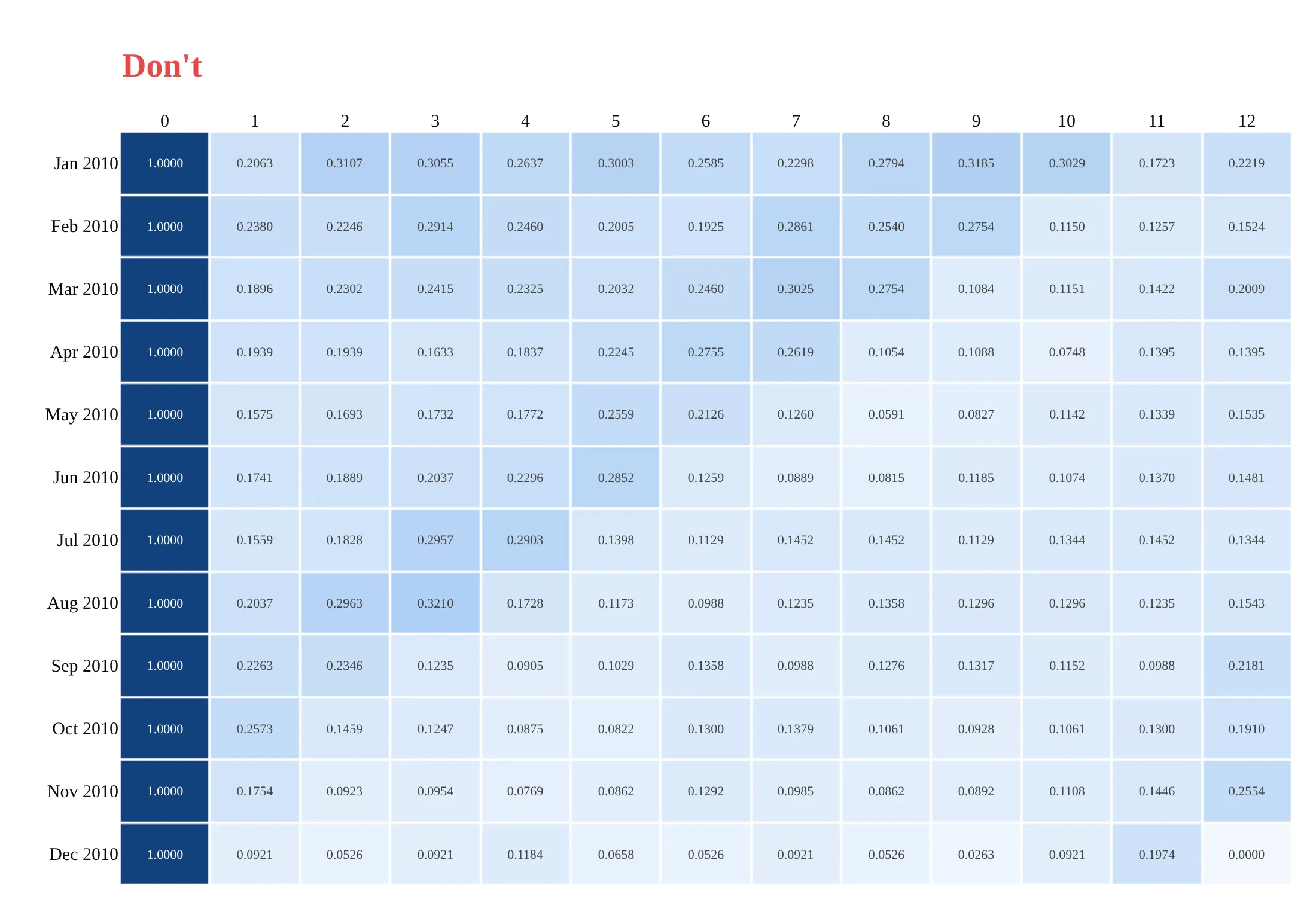
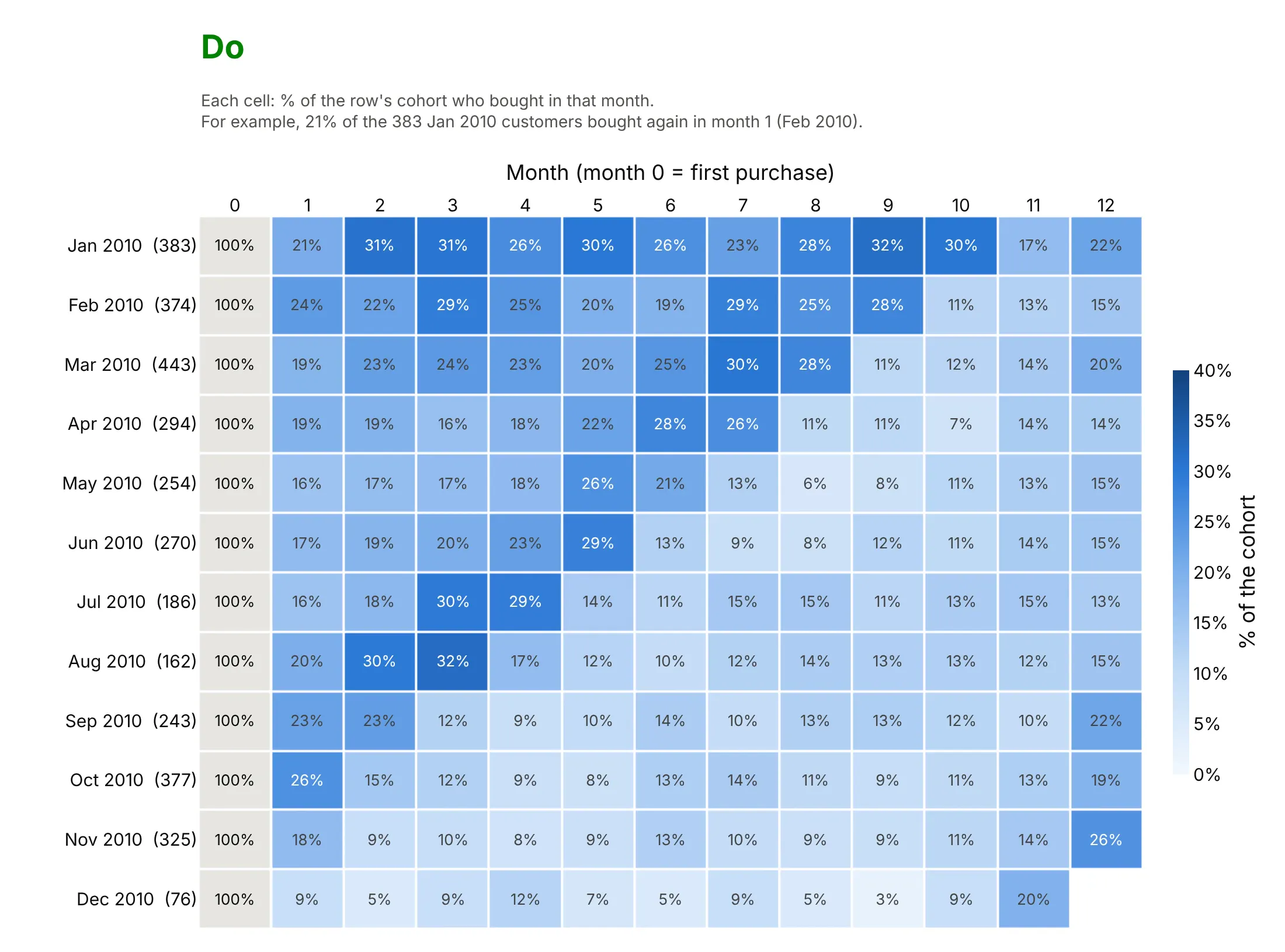
The same table can hide its message or show it, and most of the difference is the color scale and what the cells say. Here are twelve cohorts of the retail data both ways, in the same blues.
Don't put month 0 (always 100%) in the color scale, which makes every other cell look pale, draw months that haven't happened as 0%, print raw decimals that read like counts or rates without a unit, leave out the cohort sizes, or use a default serif font:
Do show month 0 as a grey 100% column outside the color scale, leave future months blank, print whole-number percentages with a % sign, put the cohort size in each row label, use one color scale for the whole table, and read one cell in plain words ("For example, ...") so nobody has to guess what a cell means:
Checklist
Do
- Say in the title what a cell is ("share of each cohort that bought in each month"), and in the subtitle what month 0 is, whether months are calendar months or 30-day periods, and one cell read out as an example ("For example, 33% of the 955 customers who first bought in Dec 2009 bought again in month 2").
- Show the cohort size next to each row, since a row of 71 customers is noisier than a row of 955.
- Leave unfinished periods blank, and treat the last diagonal with care, because a partly finished month looks like a drop.
- Use one color scale for the whole table, capped near the typical maximum.
- Mark or footnote a first cohort that contains customers who started before the data did.
- For "month N or later", use a fixed window and only the cohorts that have all of it.
- Add a weighted average row (weighted by cohort size) when readers want one number.
Don't
- Fill future cells with 0% or with the previous value.
- Print shares without a % sign, where they can be read as numbers of people.
- Compare cohorts of different sizes by color alone when some have fewer than about 100 members.
- Use a rainbow or diverging color scale for a rate that only goes from 0% upward.
- Average the percentages of cohorts of different sizes without weighting them.
More cohort retention examples
Five more charts from real public data, each with its source, the technique that makes it work and a prompt to rebuild it.
1. Revenue by cohort as a layer cake
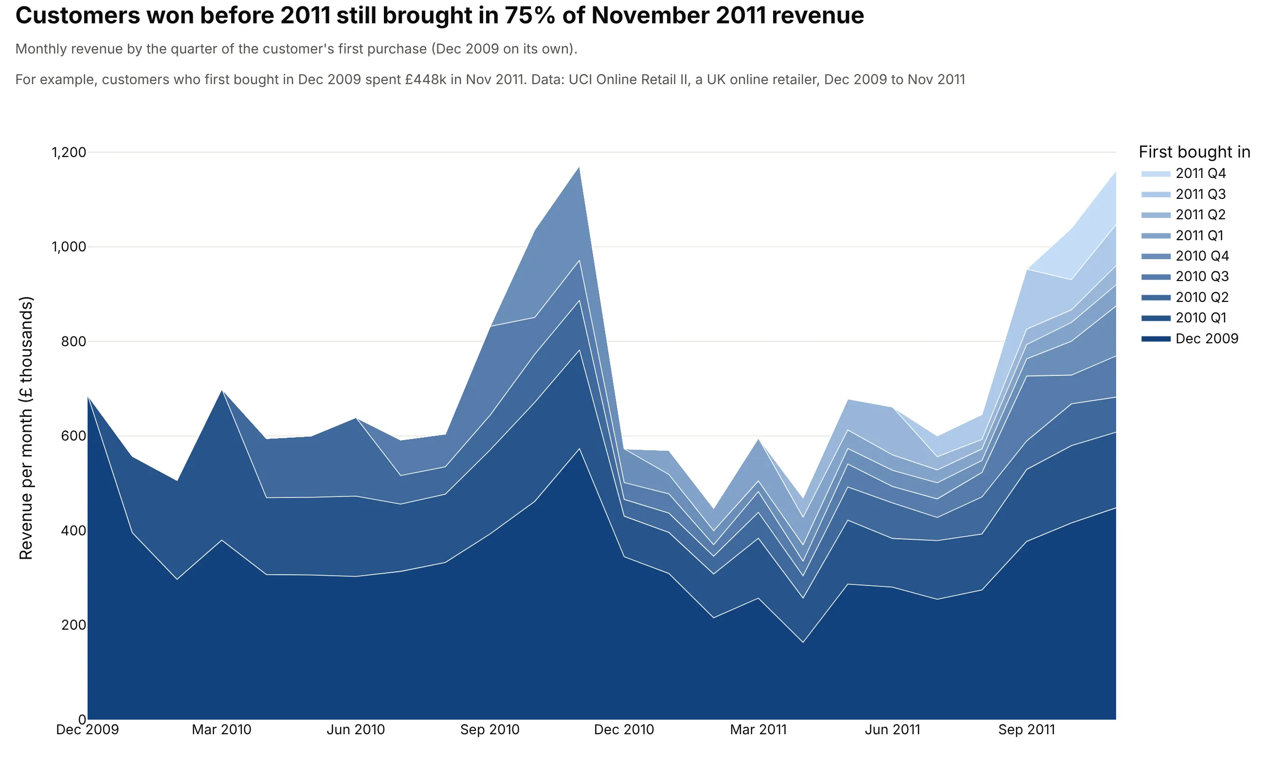
Customers whose first purchase was in 2009 or 2010 still brought in 75% of November 2011 revenue, £1.16 million. The December 2009 cohort alone is the dark layer at the bottom. Data: UCI Online Retail II, revenue as quantity times unit price for customers with an ID, £16.9 million over the 24 months.
Tip: stack the oldest cohort at the bottom in the darkest color, so the layers get lighter as the customers get newer and the oldest layer sits on the flat baseline.
Get the data from the UCI Machine Learning Repository Online Retail II (invoices of a UK onlinegiftware retailer, Dec 2009 to Dec 2011; columns: Invoice, StockCode, Quantity, InvoiceDate, Price, Customer ID, Country).Drop rows without a Customer ID, cancellations (invoices starting with C) and non-positive quantities, thenbuild a plotly layer cake: monthly revenue (Quantity * Price) stacked by the quarter of each customer's firstpurchase, the first month as its own layer, oldest layer at the bottom in dark blue, white lines between layers.Title with the share of the last full month's revenue that comes from customers won before 2011.
2. Contributors to an open-source library
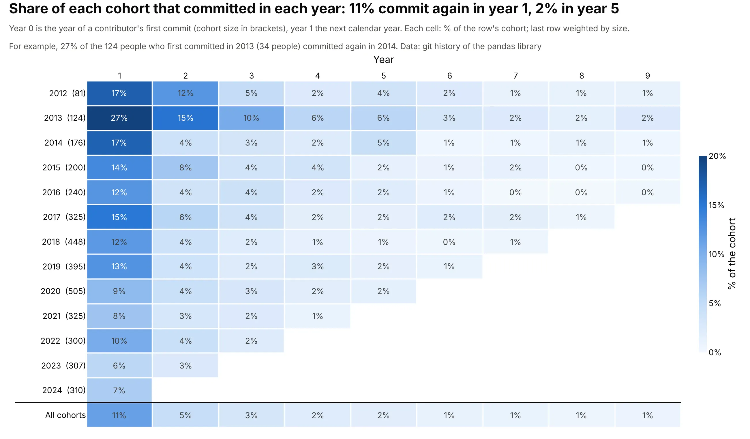
A yearly rhythm suits communities with long gaps between visits: 11% of pandas contributors commit again the next year, 5% two years on and 2% after five. The 2013 cohort, 124 people, stands out at 27% in year 1. Data: git history of the pandas library, cohort of a person = year of their first commit, authors identified by commit email address.
Tip: add a bottom row weighted by cohort size and draw a line above it, so the average reads as a summary and not as one more cohort.
Get the data from the git history of github.com/pandas-dev/pandas (clone it bare with --filter=blob:none and rungit log --format='%ae|%ad' --date=format:%Y; columns: author email, year).Build a plotly cohort retention heatmap by year of first commit (2012 to 2024), years 1 to 9 after it, each cellthe % of that row's cohort with a commit that year (with a % sign), cohort sizes in the row labels, and an"All cohorts" row weighted by cohort size under a dividing line. Blue scale capped at 20%, future years blank,a cohort and year with no commits shown as 0%. Mention that people who commit under two email addresses arecounted twice.
3. The same table by calendar month
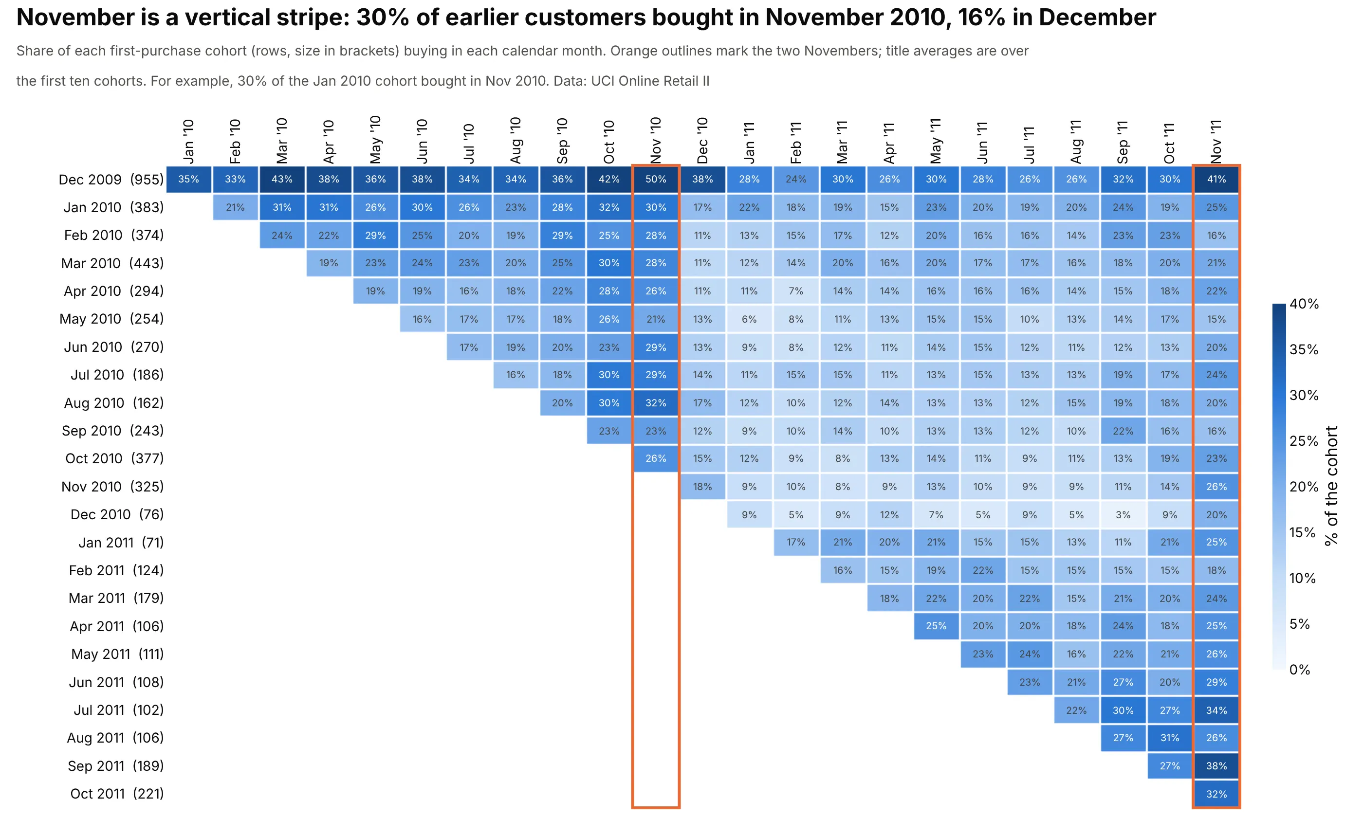
Putting calendar months on the x axis turns the diagonals of the main table into vertical stripes: the first ten cohorts averaged 30% in November 2010 and 16% in December 2010. Data: UCI Online Retail II, the same cells as the main example.
Tip: outline the stripe you want readers to see with a rect shape that covers the whole column, since the eye finds an outlined column faster than a darker one.
Get the data from the UCI Machine Learning Repository Online Retail II (columns: Invoice, InvoiceDate,Customer ID; drop guest rows without an ID and cancellations).Use plotly to draw the monthly cohort retention table with calendar months, not month numbers, alongthe x axis (Jan 2010 to Nov 2011), cohorts down the side with their sizes, one blue scale capped at 40%, andorange rectangles around the two November columns. Print the average share for November and December 2010.
4. Posts per member, not only who came back
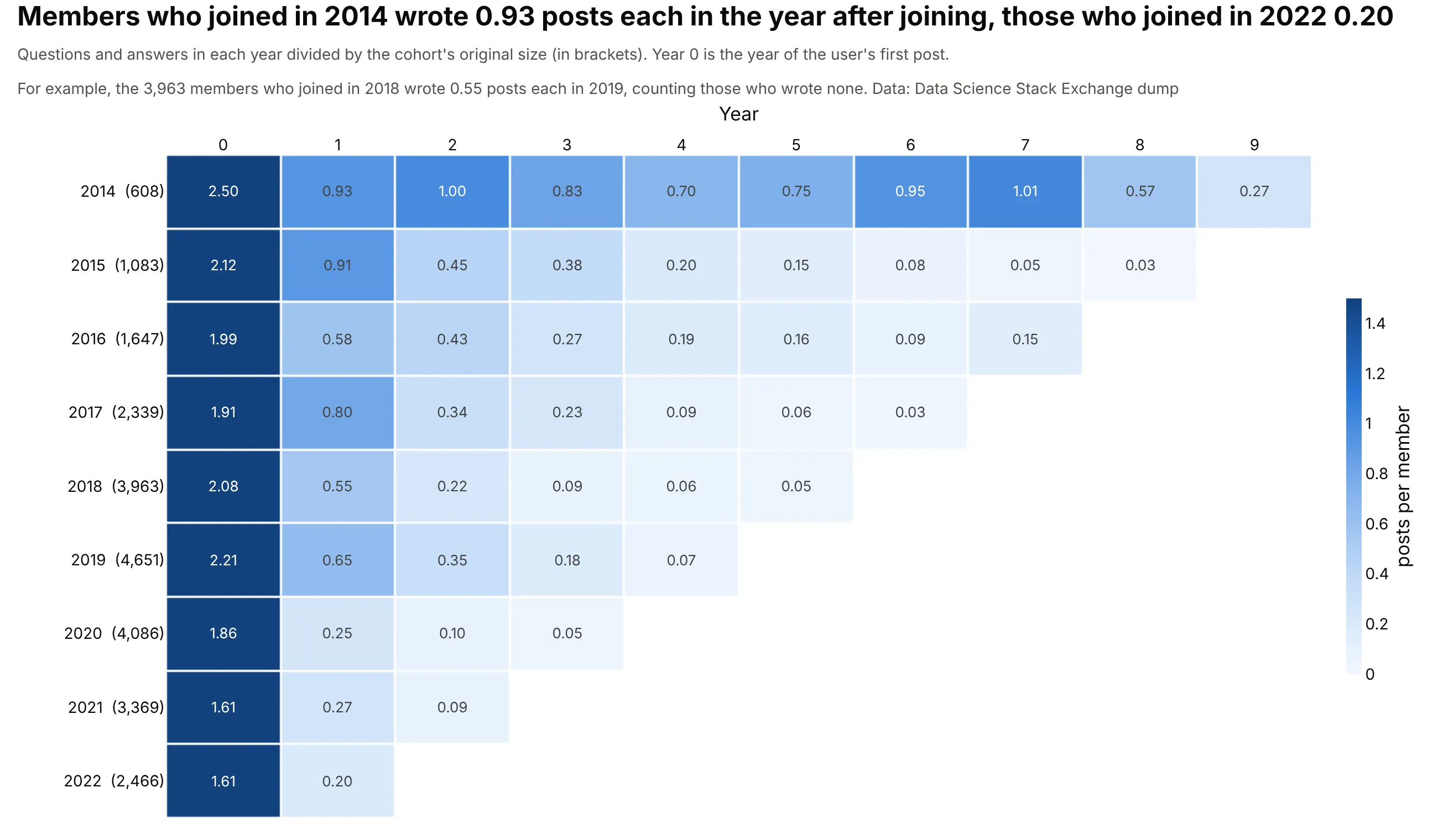
Counting posts per original member shows how much the people who stay contribute: the 2014 cohort wrote 0.93 posts each in the year after joining, the 2022 cohort 0.20. Members from 2014 also kept posting at 0.57 to 1.01 a year up to year 8. Data: Stack Exchange data dump for datascience.stackexchange.com, questions and answers.
Tip: keep the joining year (year 0) as a column, since it shows that every cohort started at about 1.6 to 2.5 posts per member, and the later differences come from who stayed.
Get the data from the Stack Exchange data dump for datascience.stackexchange.com on the Internet Archive(Posts.xml; columns: PostTypeId, OwnerUserId, CreationDate), keeping questions and answers with an owner.Build a plotly cohort table where the cohort is the year of a user's first post (2014 to 2022), the columnsare years 0 to 9 counted from it, and each cell is the cohort's posts that year divided by the cohort's size.Two decimals in each cell, blue scale capped at 1.5, cohort sizes in the row labels.
5. Cohorts defined by something other than a date
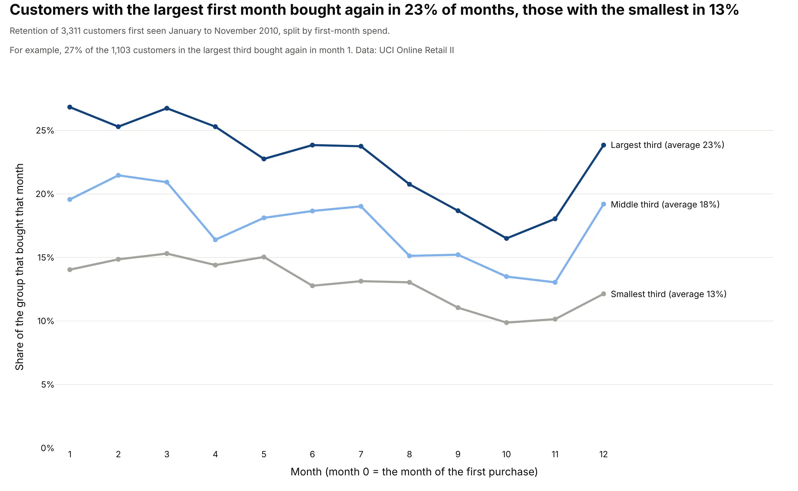
A cohort is any group that shares a starting event. Splitting the 3,311 customers who first bought from January to November 2010 into thirds by first-month spend (cut at £220 and £402) gives three curves that never cross: customers in the largest third bought in 23% of the following months, the smallest third in 13%. Data: UCI Online Retail II.
Tip: label the lines directly with their averages, and keep the three lines in one hue family ordered by size, so the ordering reads without a legend.
Get the data from the UCI Machine Learning Repository Online Retail II (columns: Invoice, InvoiceDate, Quantity,Price, Customer ID; drop guest rows, cancellations and non-positive quantities).Take the customers whose first purchase was between January and November 2010. Split them into thirds bytheir revenue in the first month, and draw a plotly line per third: the share of the group that bought ineach of the following 12 months. Label each line at its end with its average. Title with the gap between thelargest and the smallest third.
FAQ
Options to customize
A cohort retention heatmap in Plotly is a heatmap trace with a computed table, so these are the options that matter most. The full lists are in the heatmap trace reference and the area trace reference (a layer cake is a scatter trace with stackgroup).
- z: the retention matrix, with NaN or None for months that haven't happened yet, which Plotly leaves blank.
- zmin and zmax: the color range. Cap zmax near the typical maximum so ordinary cells stay readable, and keep it the same for every row.
- colorscale: a list of [position, color] pairs. Plotly's named "Blues" runs dark to light, so write the scale out when more retention should be darker.
- text and texttemplate: the label in every cell. Build text yourself (such as "21%", and "" for blank cells) and set texttemplate="%{text}", with textfont.size for readability; Plotly picks a contrasting text color.
- A second one-column go.Heatmap with a single grey colorscale and showscale=False: month 0 as a 100% column that stays out of the color scale.
- xgap and ygap: white gaps between cells, 1 to 3 px, which keeps individual cells visible.
- hovertemplate: the cohort, the month and the percentage, plus the head count from customdata.
- yaxis.autorange="reversed": the oldest cohort at the top, so the triangle points the usual way.
- xaxis.side="top" and dtick=1: the months across the top, one tick per month.
- colorbar.ticksuffix: a "%" on the colorbar without multiplying the values.
- hoverongaps=False: no tooltip on blank cells.
- add_shape(type="rect"): outlines for a row, a column, a stripe or single cells on a diagonal you want readers to see, as in the reading examples.
- stackgroup on go.Scatter: stacks the traces of a layer cake, with fillcolor per cohort and a white line between layers.
- px.imshow: a shorter route to a heatmap from a DataFrame with text_auto=True, if you don't need per-cell control.