Dual-Axis Charts - A Complete Guide

TL;DR

• A dual-axis chart draws two series with different units on one time or category axis, one measured on the left y axis and one on the right, such as rain in inches and temperature in degrees for the same months.
• Dual-axis charts are also known as dual y-axis charts, double y axis charts, secondary axis charts and twin axes (matplotlib's twinx), and when one series is bars and the other a line they are called combination or combo charts. They are similar to line charts, small multiples and Pareto charts, which are a kind of combo chart.
• They are at their best for time series and sensor logs, where you want to see which signals rise and fall together and whether one lags the other. Some data visualization writers dislike them because hand-picked ranges can make either line look flat; with Plotly's default autorange each axis fits its own data.
• You can make a dual-axis chart with Plotly in Python with make_subplots(specs=[[{"secondary_y": True}]]) and secondary_y=True on the second trace, or in JavaScript with a yaxis2 that has overlaying: "y". Since plotly.js 4.0 (Plotly for Python 7.0), the second axis's ticks snap to the first axis's gridlines by default (tickmode="sync"), so you get one clean grid.

What is a dual-axis chart?

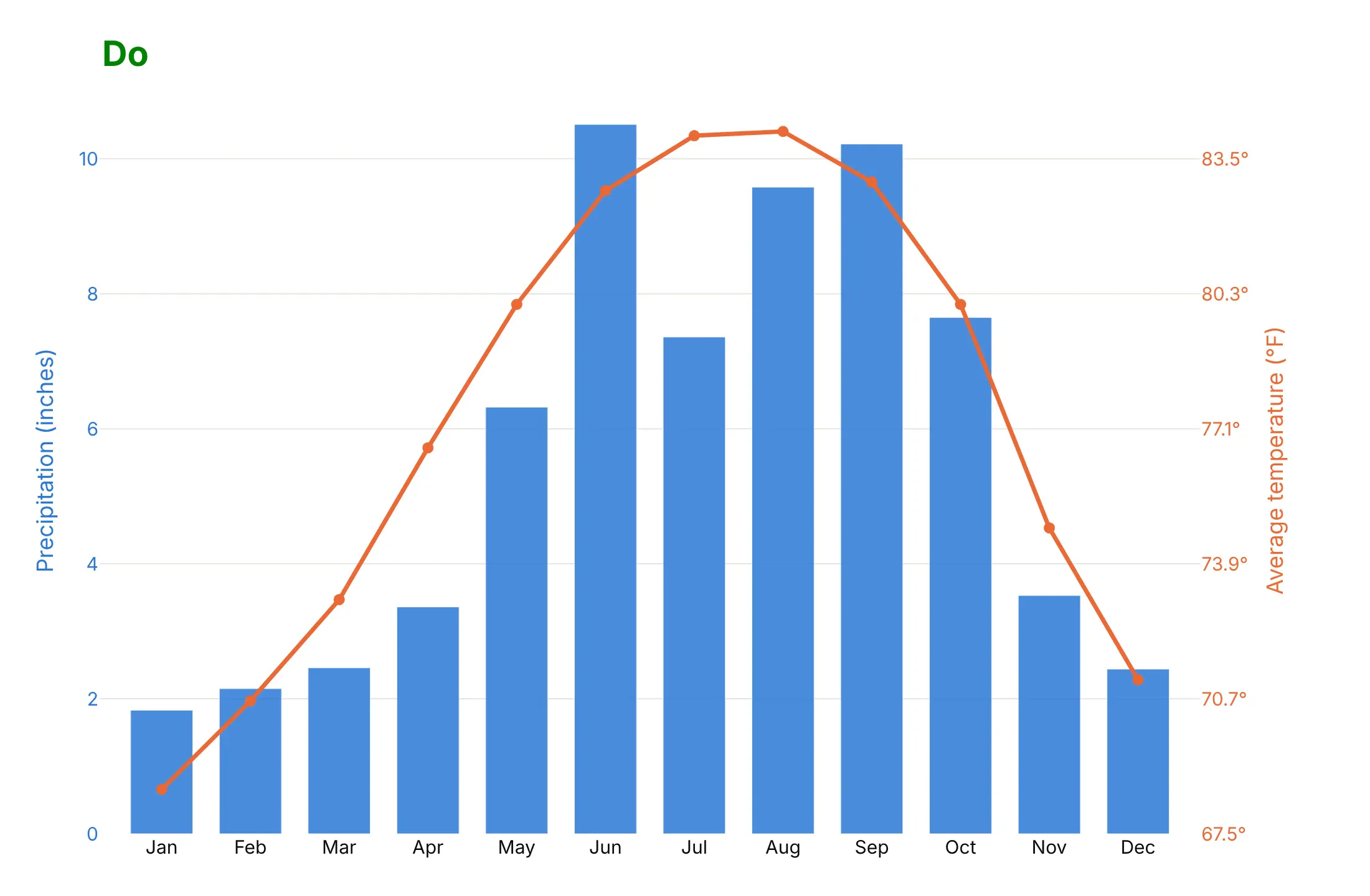
Dual-axis charts look like this:

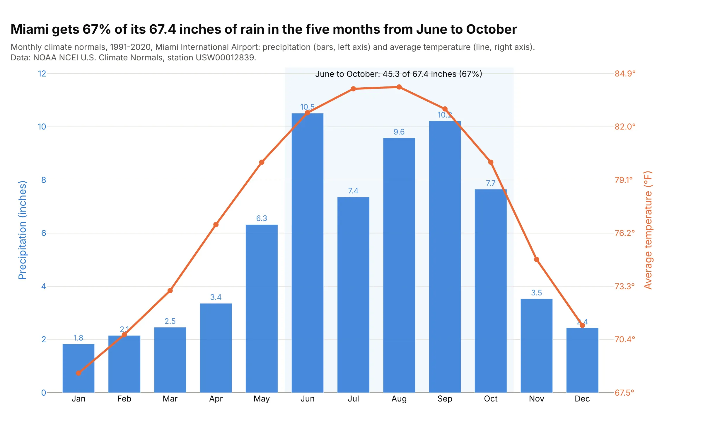
Data: U.S. Climate Normals 1991-2020 from the National Oceanic and Atmospheric Administration's National Centers for Environmental Information (NOAA NCEI), Miami International Airport (station USW00012839).

How do you read a dual-axis chart? In the example above, notice these things:

• Each series has its own axis, and the colors tell you which: the blue bars are precipitation in inches on the blue left axis, and the orange line is average temperature in °F on the orange right axis.
• Read each series against its own axis. June's bar reaches 10.5 on the left (10.51 inches of rain), and August's dot sits at about 84 on the right (84.2°F, the warmest month).
• The point of putting them together is the season. June to October brings 45.3 of Miami's 67.4 inches of rain a year, 67%, and each of those months averages above 80°F, so the wet season and the hot season line up.
• There is one set of gridlines. Both axes use Plotly's default autorange, and the right axis's ticks sit on the left axis's gridlines, so the grid doesn't double up.

It's often used for charts like these:

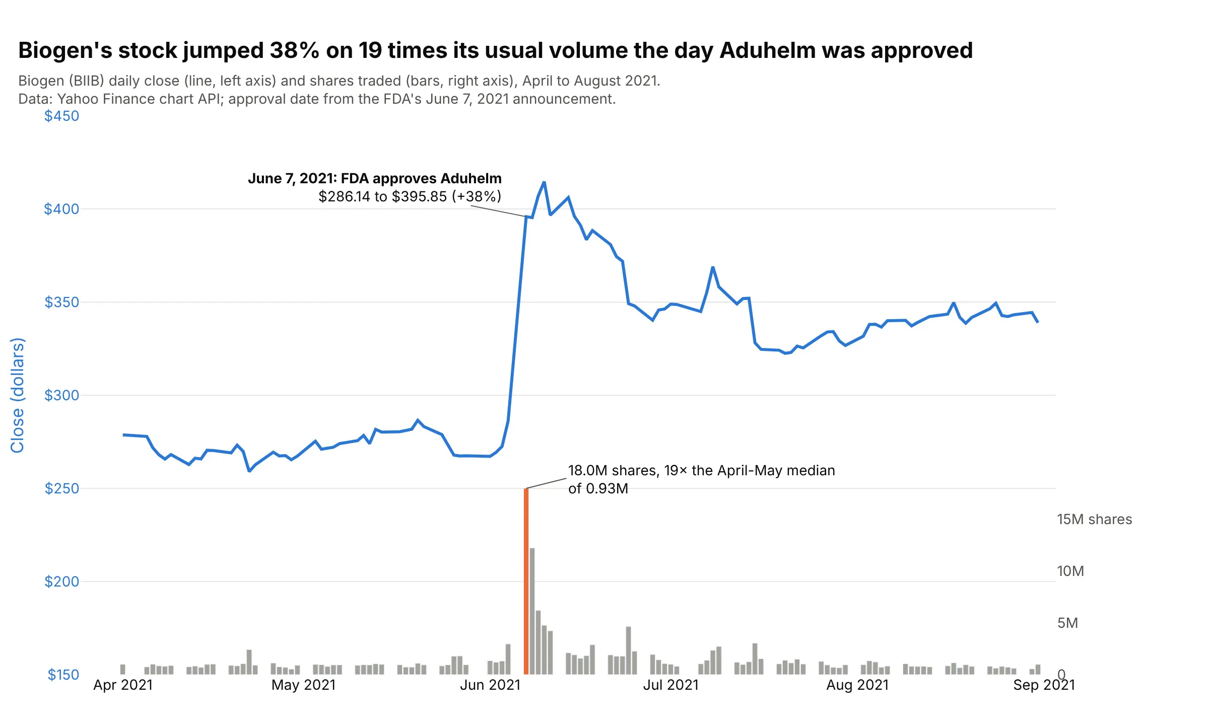
Price and volume. Biogen's stock rose 38% on June 7, 2021, the day the US Food and Drug Administration (FDA) approved Aduhelm, on 18.0 million shares, 19 times its usual daily volume. Data: Yahoo Finance chart API (ticker BIIB); approval date from the FDA's announcement, as reported by the Regulatory Affairs Professionals Society (RAPS).

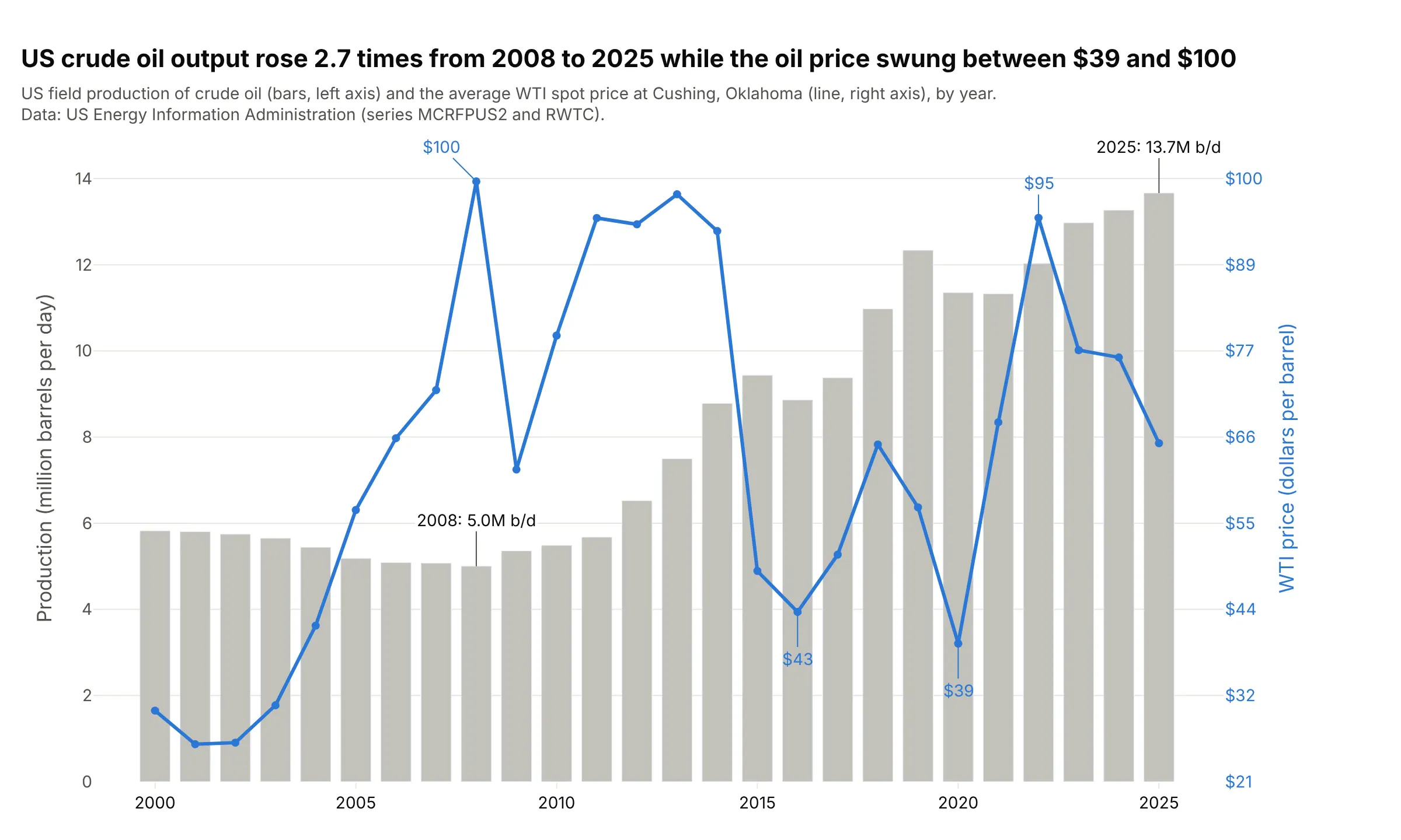
Bar and line combo charts. US crude oil production rose 2.7 times from 2008 to 2025, from 5.0 to 13.7 million barrels a day, while the yearly average price of West Texas Intermediate (WTI) crude swung between $39 and $100. Data: US Energy Information Administration (EIA), series MCRFPUS2 and RWTC.

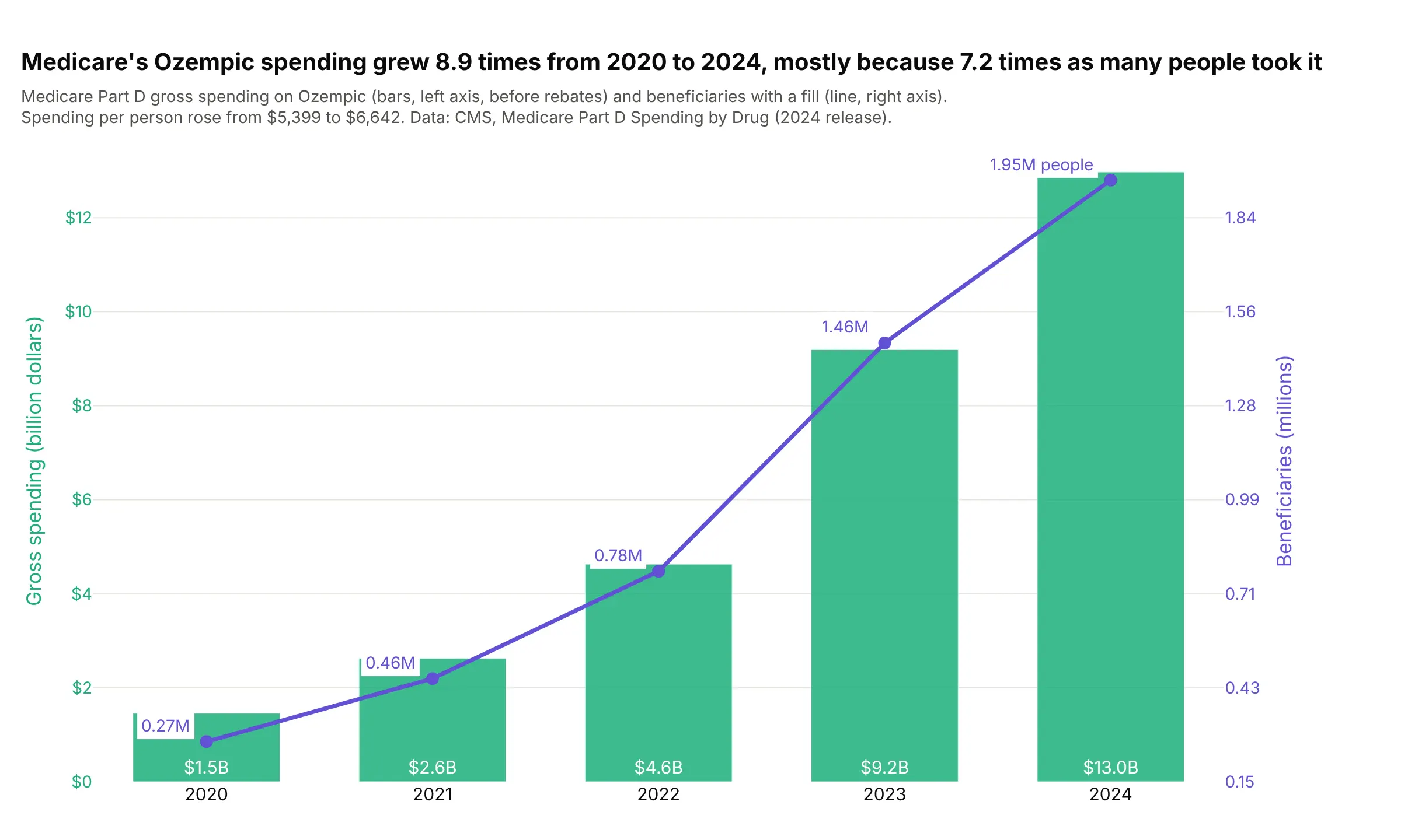
Spending and patients. Medicare's gross spending on Ozempic grew 8.9 times from 2020 to 2024, to $13.0 billion, mostly because 7.2 times as many people filled a prescription, 1.95 million in 2024. Data: Centers for Medicare & Medicaid Services (CMS), Medicare Part D Spending by Drug.

A short history

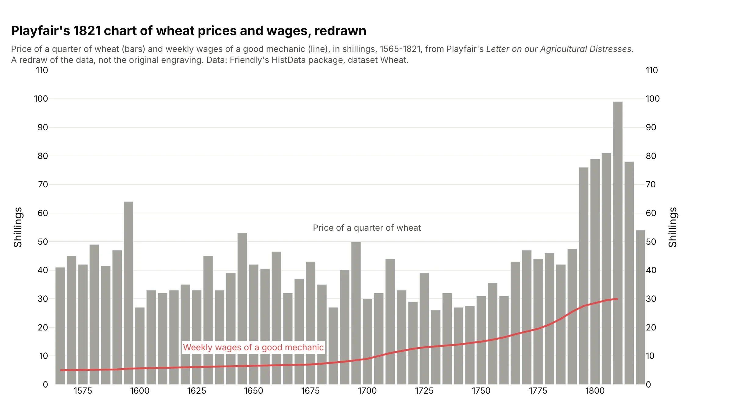
William Playfair published a chart in 1821 that put the price of wheat as bars and the weekly wages of a good mechanic as a line over 256 years. Michael Friendly's HistData documentation calls it "a classic in the history of data visualization" that "commits the sin of showing two non-commensurable Y variables on different axes", and suggests plotting the ratio as well (Friendly and Denis 2005). This is Playfair's data, redrawn:

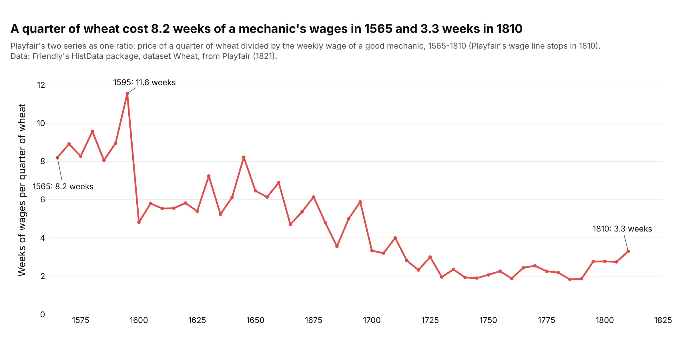
Another way to see it: dividing one series by the other answers the question Playfair was asking, how many weeks of work a quarter of wheat cost, on a single axis. It fell from 8.2 weeks in 1565 to 3.3 in 1810.

Climate scientists built a second axis into a standard chart. Walter and Lieth's 1960 Klimadiagramm-Weltatlas fixed the scale at 2 mm of precipitation per °C, so that a month where the rain line falls below the temperature line counts as dry (climatol documentation); example 7 below draws two of them. Engineers and scientists use the same idea for measured signals, and the tools they use build it in: MATLAB's yyaxis is documented as "Create chart with two y-axes", matplotlib has twinx and Plotly has secondary_y.

Why some people dislike dual-axis charts

The critics' argument is that each axis range is a choice, and nothing ties the two choices together. Stephen Few's 2008 article "Dual-Scaled Axes in Graphs: Are They Ever the Best Solution?" concluded "I can't think of a single case when there isn't a better solution", and ggplot2 only allows a second axis that is "a one-to-one transformation of the primary axes", such as °C and °F. Here is the case at its strongest, with the same US crude oil production and WTI price data drawn three times:

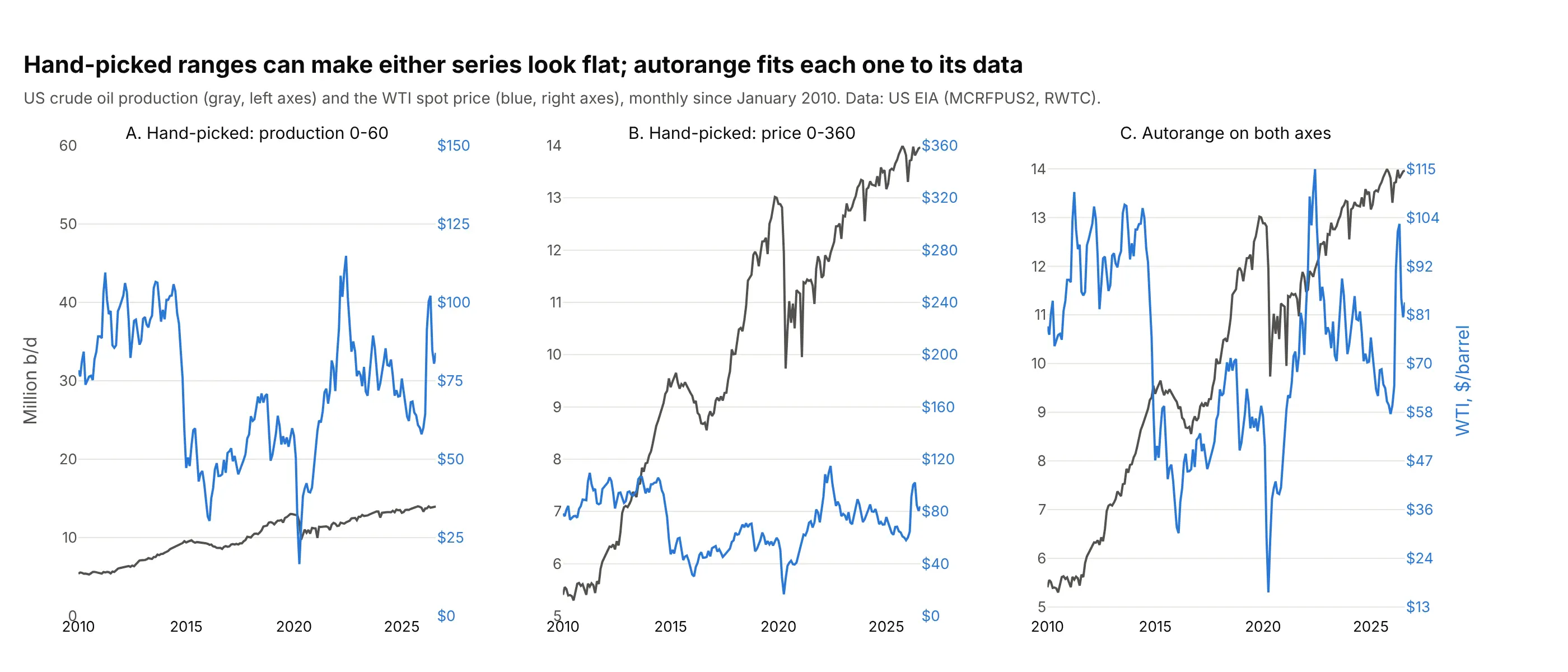
Panels A and B are misleading, and they are misleading for the same reason: someone picked a range that squashes one of the series. Panel C uses Plotly's default autorange on both axes, which fits each axis to its own data, and both series are readable: production climbed most of the time and the price went up and down. Where the two lines cross in panel C still means nothing, because the two scales are independent, and that is the one thing to keep in mind when you read any dual-axis chart.

Why I like dual-axis charts

Many people in data visualization don't like them, but I disagree, and I use them a lot for time series where I'm trying to see how different variables rise and fall together. Putting two signals on top of each other lets you see three things that are hard to see in separate panels: which peaks and troughs line up, whether the relationship holds over the whole period or only part of it, and whether one signal moves first.

This is a chart from my post Analyzing Apple Health Data in Plotly Studio, made in Plotly Studio:

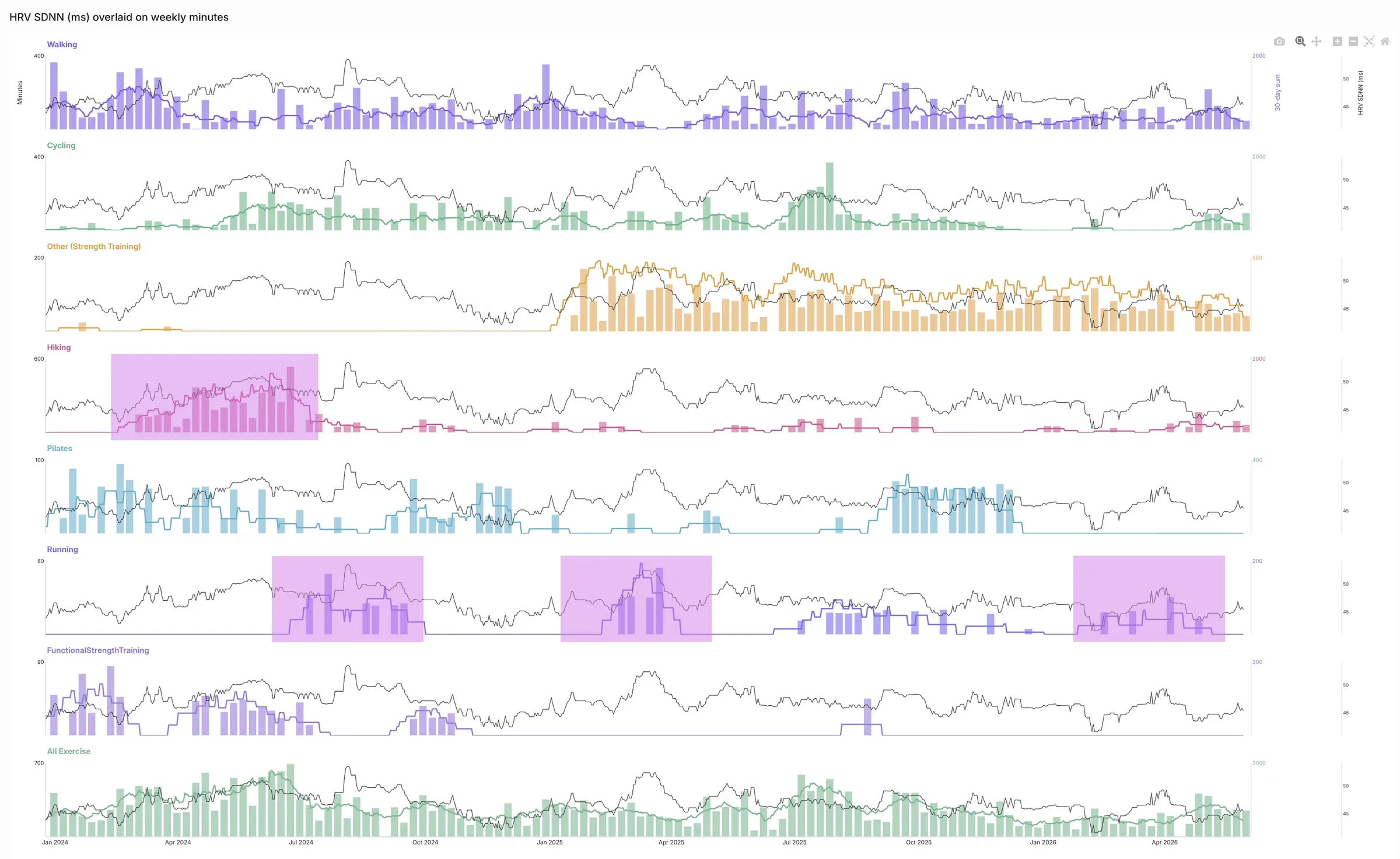
Data: one person's Apple Health export, from Chris Parmer's post.

Each panel puts weekly exercise minutes on one axis and heart rate variability (HRV, measured as SDNN, the standard deviation of the intervals between normal heartbeats) on another, and the shaded periods make the pattern easy to check: HRV "increased every time she introduced running into her training". In the same analysis, VO2 max (the most oxygen the body can use during exercise) "appears to be a lagging indicator", rising only after a long stretch of hiking and cycling to work, and resting heart rate (in beats per minute, BPM) "decreased about 5 BPM from 60BPM to 55BPM during the intense period of hiking training" and went back up afterwards. Seeing a delay like that is exactly what a second axis is good at.

Engineering and science data works the same way, and examples 8 to 10 below are a battery test, a tide gauge and the Texas grid. On a hot August week in Texas, electricity demand on the Electric Reliability Council of Texas (ERCOT) grid tracks the temperature at Dallas/Fort Worth (DFW) airport hour by hour, and it peaks a little later each day (example 10 below). You can put a number on that delay with cross-correlation, the correlation between one series and the other shifted by each possible lag:

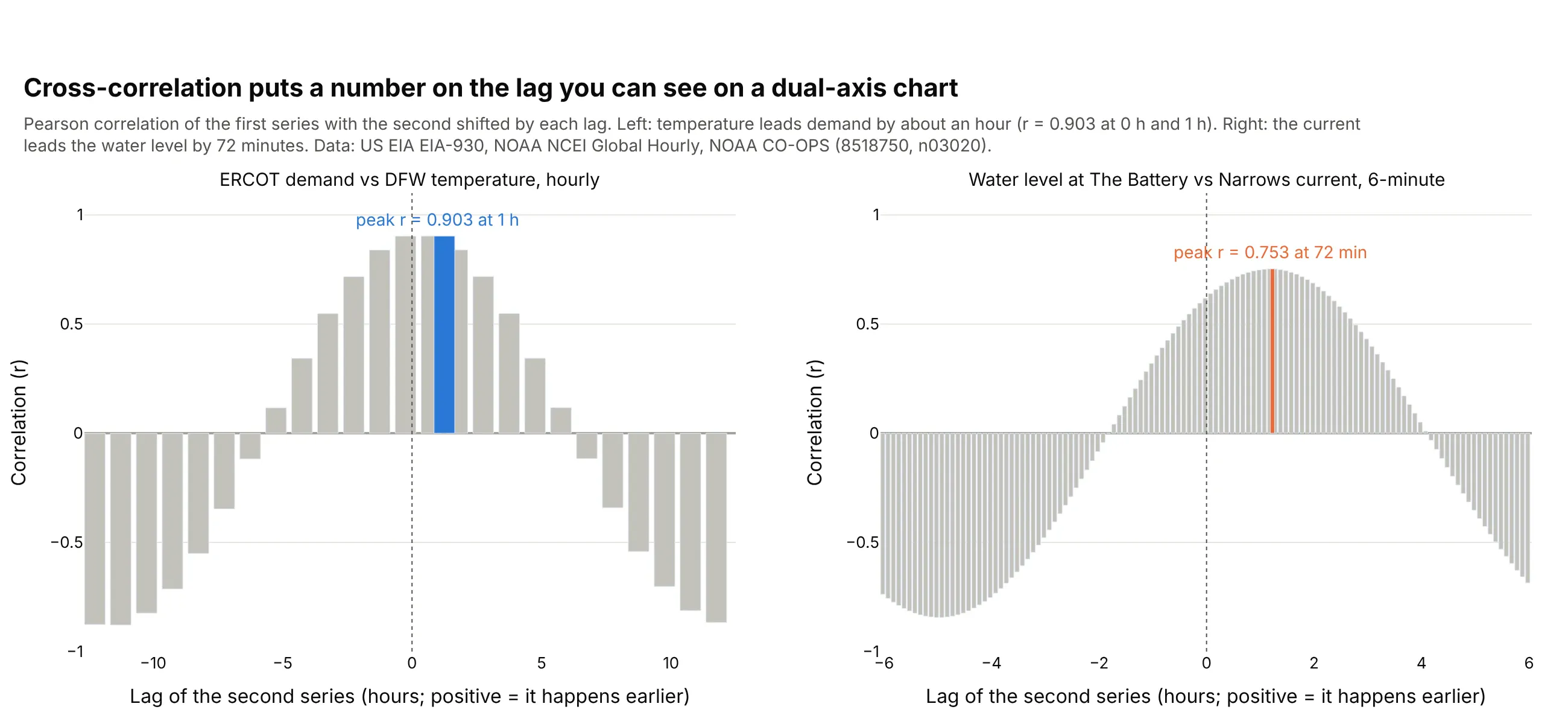
For the Texas week the correlation is 0.903 at both 0 and 1 hours, so the lag is about an hour at hourly resolution, and on six of seven days demand peaked one or two hours after the temperature did. In New York Harbor the delay is clearer: the tidal current at The Narrows runs 72 minutes ahead of the water level at The Battery (example 9).

Another way to see it: plot one signal against the other, one dot per hour in time order. This is a connected scatter plot, which mathematicians call a parametric plot because each point is (x(t), y(t)) with time t as the parameter; in dynamical systems the same picture is a phase portrait. When one signal lags the other, the path out and the path back differ and the curve makes a loop, which is what hysteresis looks like when it comes from a time lag:

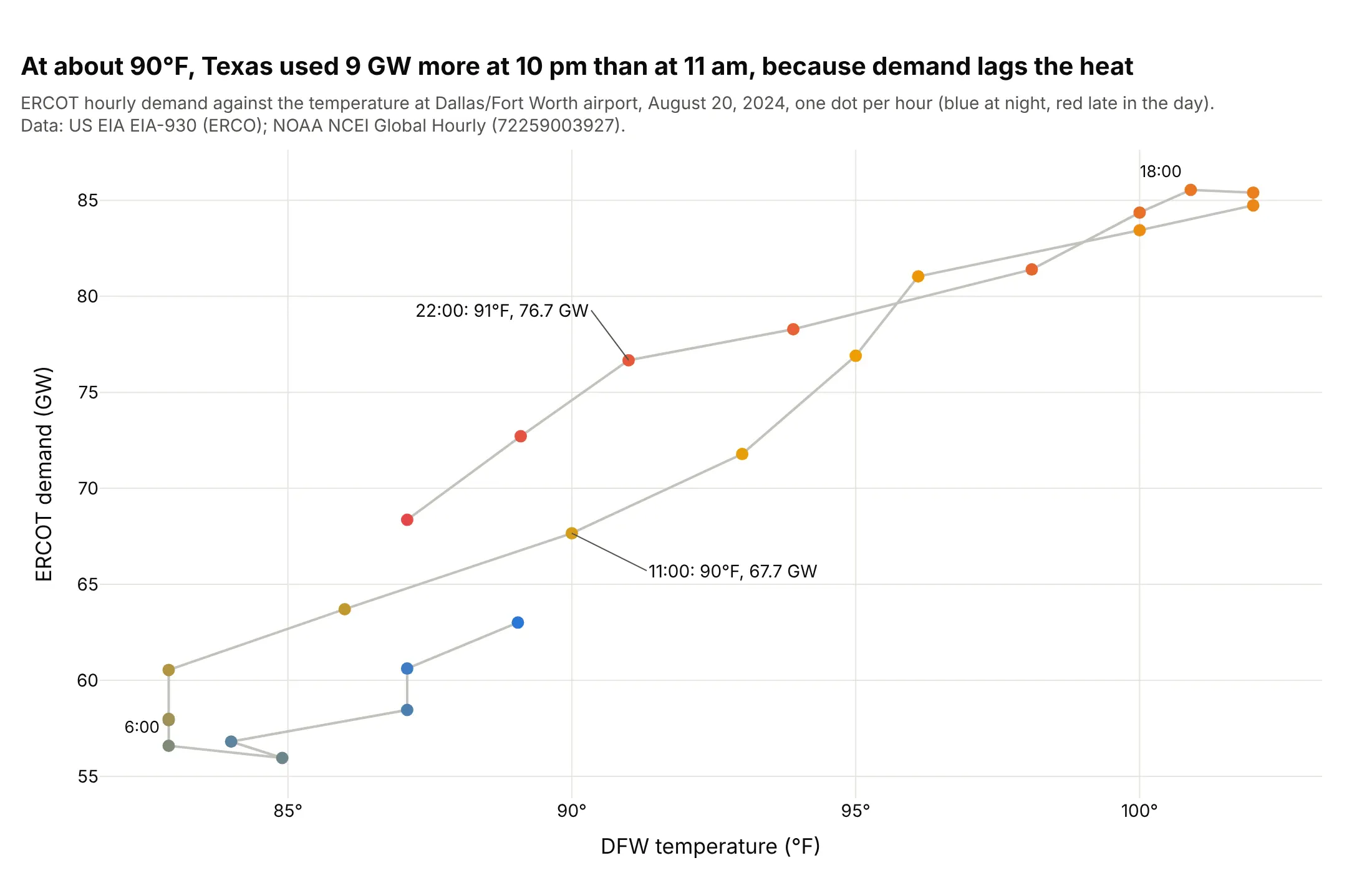
At about 90°F, Texas used 9.0 gigawatts (GW) more at 10 pm than at 11 am, because demand lags the temperature.

What keeps these charts clean is the styling, not the range. Color each axis like its line, keep one set of gridlines (Plotly does this by default now), and draw the line on top of any bars. Some people like to stagger the two lines, one in the upper part of the chart and one in the lower part, by setting the ranges by hand, as in examples 1 and 4 below. That's a nice touch when the lines would otherwise tangle, but it's a matter of preference.

Alternatives to a dual-axis chart

Here's the same crude oil data drawn four ways. Each one is good at something different:

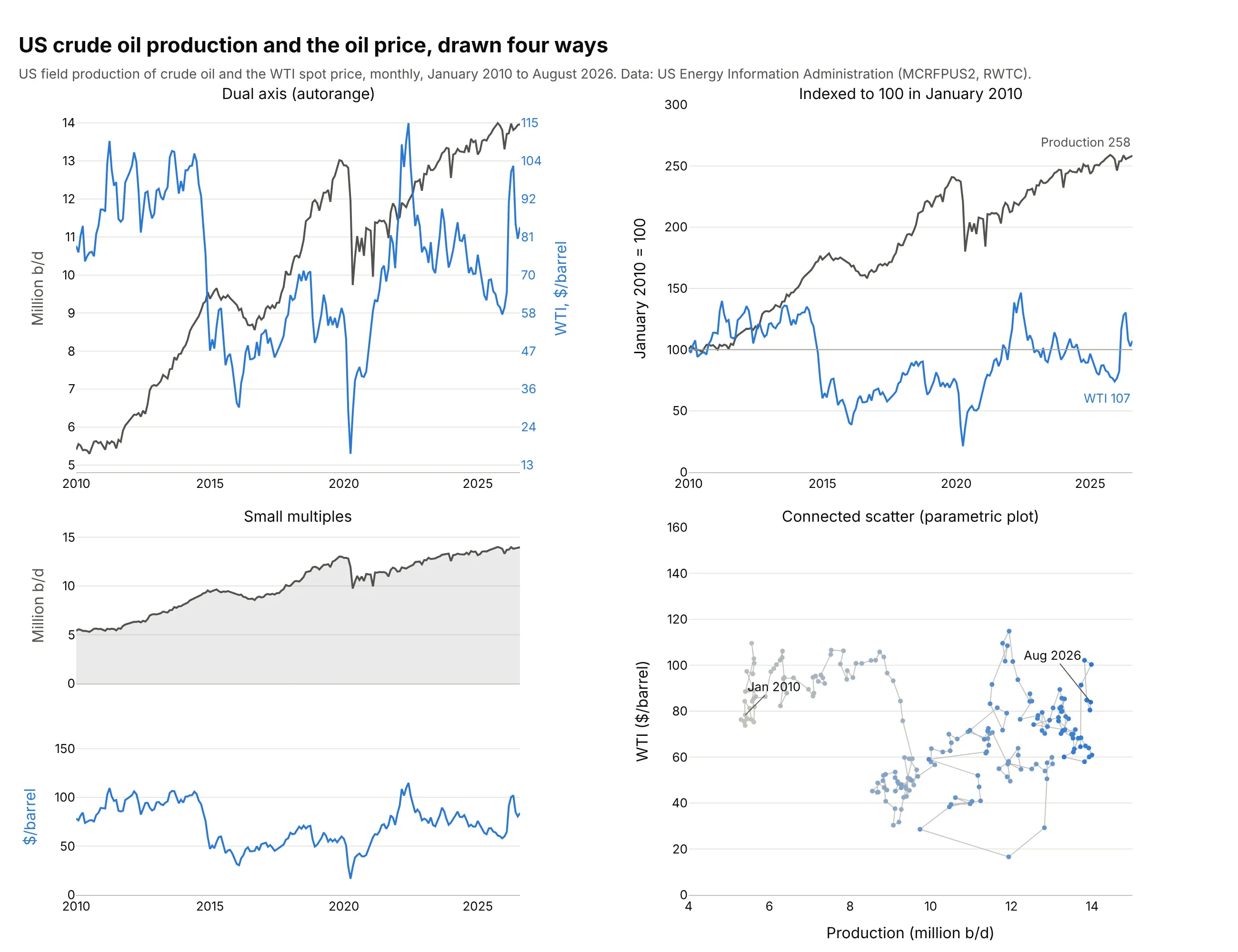
• Dual-axis chart (good for seeing both in their own units, in one place). You can read the actual production and price at any month and see which moves happened together, like the 2020 drop in both.
• Indexed line chart (good for comparing growth). Dividing both series by their January 2010 value puts them on one axis in percent: production ended at 258 and the price at 107, so output grew 2.6 times while the price ended about where it started. This is Few's suggestion for time series, and the line chart guide shows it too. You lose the units.
• Small multiples (good for many signals). Panels stacked with a shared time axis keep each series in its units and scale to five or ten signals. It's Plotly's make_subplots(rows=2, shared_xaxes=True); see the small multiples guide. Lining up peaks across panels takes more effort.
• Connected scatter or parametric plot (good for the relationship itself). Price against production, one dot per month, shows that output kept rising whatever the price did, and it shows lags as loops (Haroz, Kosara and Franconeri 2016 studied how people read them). The time order is harder to follow; see the scatter plot guide.

How to make a dual-axis chart

With AI

ChatGPT, Claude Code, GitHub Copilot, Cursor and other AI tools are excellent at writing Plotly code. Name Plotly in the prompt, and say which series goes on which axis and how each axis should look:

With Plotly Studio

Plotly Studio is a desktop app where you point an AI at a dataset and it builds charts and a Dash app around your questions. Ask for a dual-axis chart the same way:

Show hourly ERCOT electricity demand as a blue line and the Dallas temperature as a red line on a second y axis, one week in August 2024, and mark each day's peak of both.

Make a dual-axis chart in Python or JavaScript

This is the code AI tools write under the hood. In Python, make_subplots with secondary_y gives you a second y axis on the right, and the Plotly multiple axes documentation covers third and fourth axes:

Traces on the secondary axis are drawn on top of the primary ones, so put the line there and the bars on the left. The plotly.js 4.0.0 changelog (August 24, 2026) lists the change as "Set default layout.axis.tickmode to 'sync' when axis is overlaying", and Plotly for Python 7.0.0 ships that version. With sync, the second axis's ticks sit on the first axis's gridlines and are labeled from its own range, so the labels may not be round numbers; set tickformat (for example ".1f") to choose how many decimals they show. tickmode="auto" brings back an independent set of ticks.

In JavaScript, the second axis is a yaxis2 with overlaying: "y", and the trace points at it with yaxis: "y2":

Share it

Every Plotly chart has a Share chart button (the cloud icon in its toolbar) that uploads it to Plotly Cloud and gives you a link. Only you can see it until you change its visibility.

For a live app, put the chart in a Dash app and publish it with the Plotly Cloud command-line interface (CLI). Coding agents can run these commands for you:

If your data has to stay in your own cloud or data center, publish to Dash Enterprise instead.

Dos and don'ts

Most dual-axis charts that are hard to read have the same problems: you can't tell which line goes with which axis, and two grids fight each other. Here is the Miami climograph both ways.

Don't draw both series in the same color with no axis titles, so the reader has to guess which axis is which, turn on a second set of gridlines that don't line up with the first, let the bars cover the line, or leave months as numbers in a default serif font:

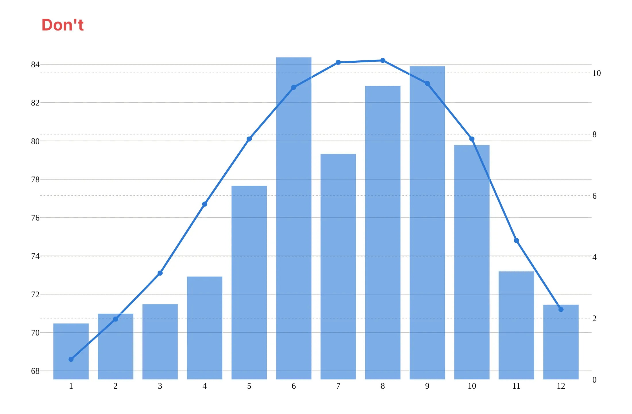
Do color each axis title and its tick labels like its series, keep Plotly's autorange and its synced gridlines (one grid), draw the line on top of the bars, and write units in the axis titles:

Checklist

Do

• Color each axis title and tick labels like its series, or label each line directly.
• Keep one set of gridlines: Plotly's default tickmode="sync" with showgrid=False on the second axis.
• Draw the line over the bars by putting it on the secondary axis.
• Say in the subtitle which series is on which axis.
• Look for what rises and falls together and for delays, and measure a lag with cross-correlation before you claim one.

Don't

• Read meaning into the exact point where two lines cross; the two scales are independent.
• Squash one series with a hand-picked range to make a point.
• Use a second axis when the two series share a unit; put them on one axis.
• Add a third or fourth axis unless each line is labeled and readers know the signals.

Options to customize

A dual-axis chart in Plotly is two traces on two y axes, the second one overlaying the first, so these are the options that matter most. The full lists are in the make_subplots reference and the layout.yaxis reference.

1. make_subplots(specs=[[{"secondary_y": True}]]): creates a figure with a second y axis on the right.
2. secondary_y=True in add_trace and update_yaxes: puts a trace on, or styles, the second axis.
3. yaxis2=dict(overlaying="y", side="right") and yaxis="y2" on a trace: the same thing without make_subplots, and how plotly.js does it.
4. tickmode="sync": places the second axis's ticks on the first axis's gridlines; the default for overlaying axes since plotly.js 4.0 and Plotly for Python 7.0. Use "auto" for independent ticks.
5. tickformat: the number of decimals on synced tick labels, like ".0f" or ".2f".
6. showgrid=False on the secondary axis: one set of gridlines instead of two.
7. title.font.color, tickfont.color: color each axis like its series, so readers know which is which.
8. range (optional styling): set the ranges by hand to stagger the two lines, one high and one low, or to hang bars from the top with a reversed range, as in examples 1 and 4. Autorange is the default.
9. anchor="free", autoshift=True, shift, position: a third or fourth y axis next to the second one.
10. tickprefix, ticksuffix: units on the ticks, like $, ° or %.
11. go.Scattergl: WebGL traces, for hundreds of thousands of markers; for lines, the SVG (scalable vector graphics) go.Scatter was faster in our test (see the FAQ).

More dual-axis chart examples

Ten more dual-axis charts built from real public data, from hydrology and climate to markets, a battery test and the power grid, each with its source, the technique that makes it work and a prompt to rebuild it.

1. A Hurricane Harvey hydrograph

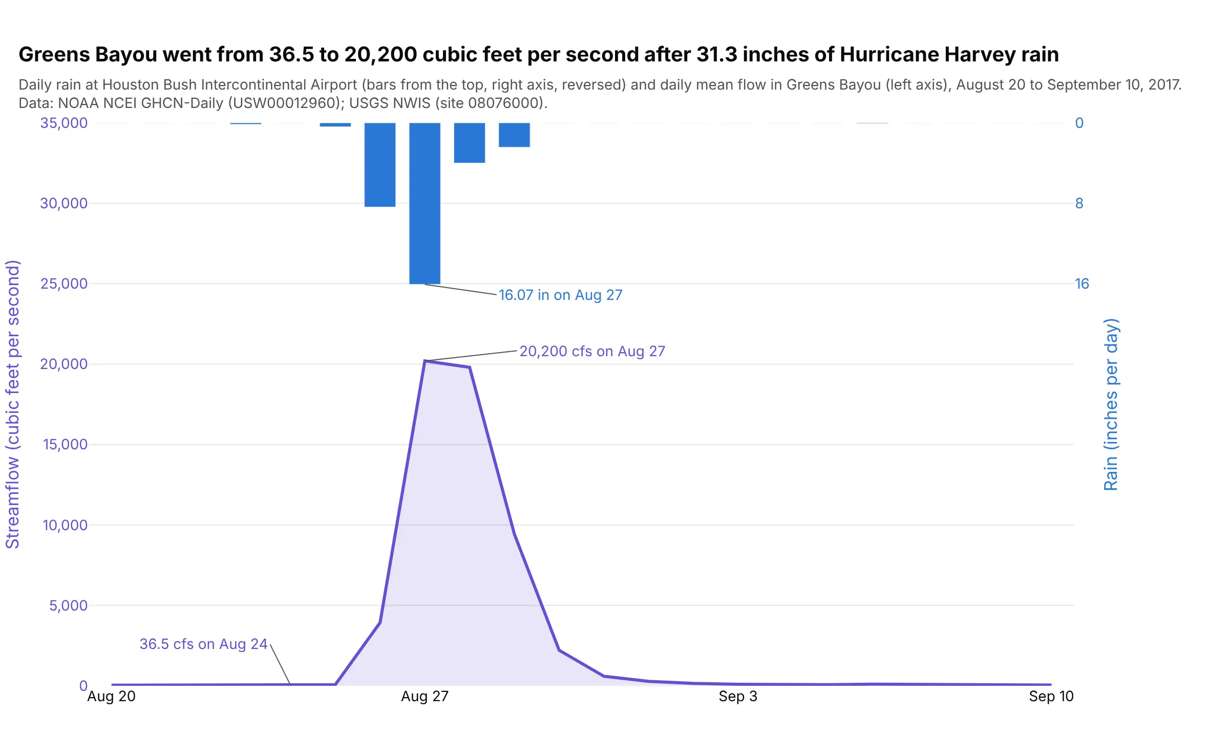
Greens Bayou near Houston went from 36.5 to 20,200 cubic feet per second in three days, after 31.3 inches of rain fell at Bush Intercontinental Airport from August 25 to 29, 2017. The flow peaked on the same day as the rain, and the chart shows how fast it fell away afterwards. Data: NOAA NCEI Global Historical Climatology Network Daily (GHCN-Daily), station USW00012960, and the US Geological Survey (USGS) National Water Information System (NWIS), site 08076000.

Tip: hanging the rain bars from the top with a reversed axis is the hydrologists' convention and an optional styling choice that keeps the bars clear of the flow line.

2. The warmest year in NASA's record, in two units

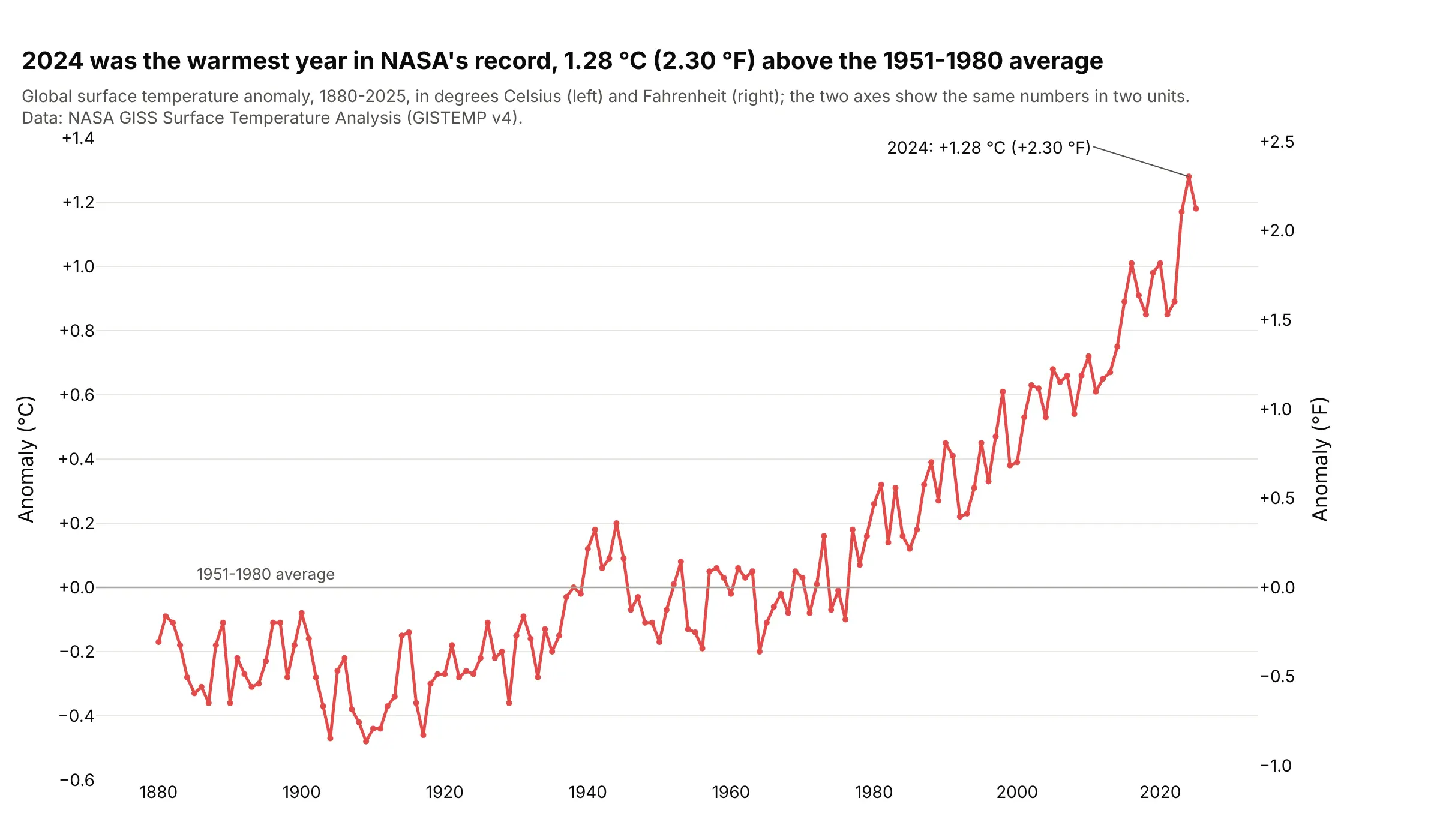
2024 was 1.28 °C, or 2.30 °F, above the 1951-1980 average, the highest in the National Aeronautics and Space Administration's (NASA's) record since 1880. The right axis converts the left one exactly, so it only saves readers the arithmetic. Data: NASA Goddard Institute for Space Studies (GISS) Surface Temperature Analysis (GISTEMP v4).

Tip: a conversion axis is the one case where the second range has to be set from the first (here times 9/5), and an invisible trace makes Plotly draw it.

3. Gas storage and the Henry Hub price

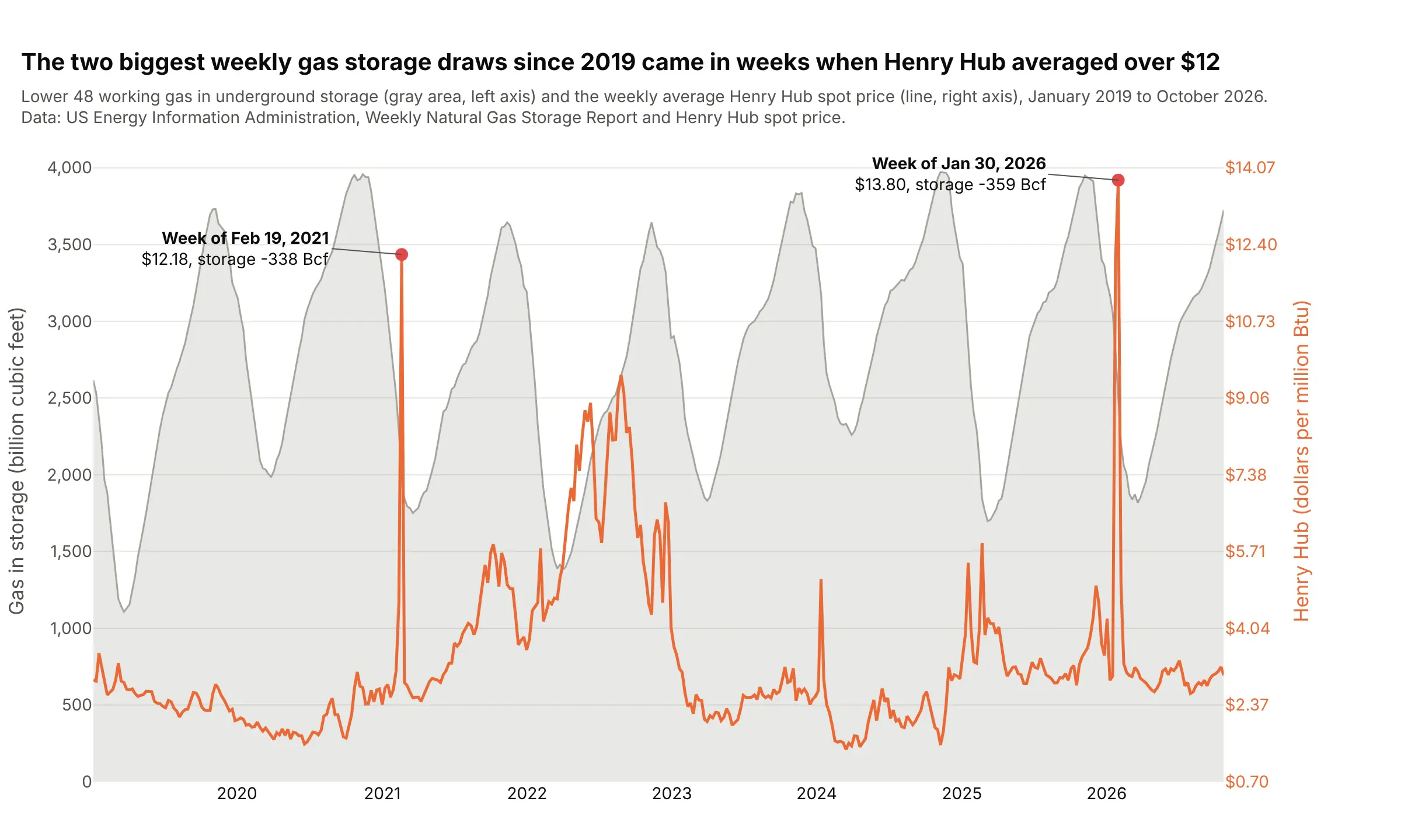
The two biggest weekly storage draws since 2019, 359 billion cubic feet in the week of January 30, 2026 and 338 in the week of February 19, 2021, came in weeks when Henry Hub averaged over $12, two of the three such weeks in the data. Gas traders read the storage sawtooth against the price because the cold snaps show up in both. Data: US EIA, Weekly Natural Gas Storage Report and Henry Hub spot price.

Tip: mark the events the chart is about on both series, so readers see them happen at the same moment.

4. The S&P 500 and the VIX in the April 2025 sell-off

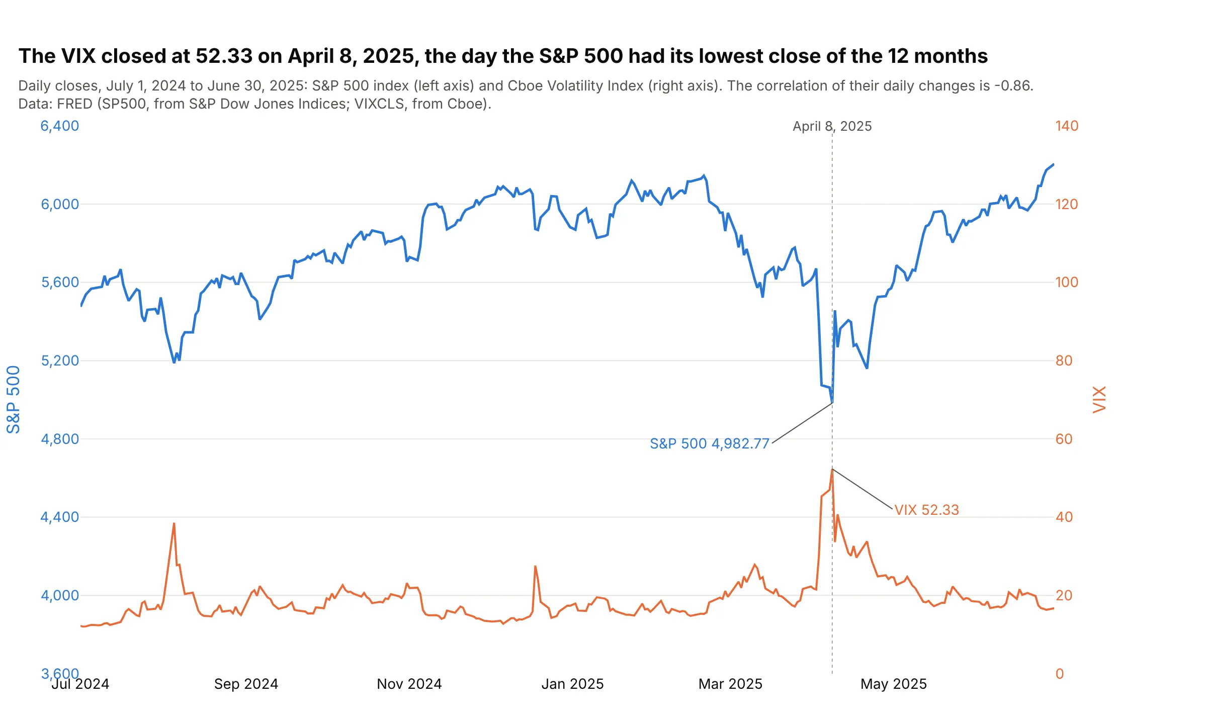
On April 8, 2025, the Cboe Volatility Index (VIX) closed at 52.33, its high for the 12 months, and the S&P 500 closed at 4,982.77, its low. Daily changes in the two had a correlation of -0.86 over the year. Data: Federal Reserve Economic Data (FRED), series SP500 (from S&P Dow Jones Indices) and VIXCLS (from Cboe).

Tip: this one shows the optional staggered style: hand-set ranges keep the index in the upper half and the VIX in the lower half, so the lines only meet on the day that matters.

5. Three climate records on three y axes

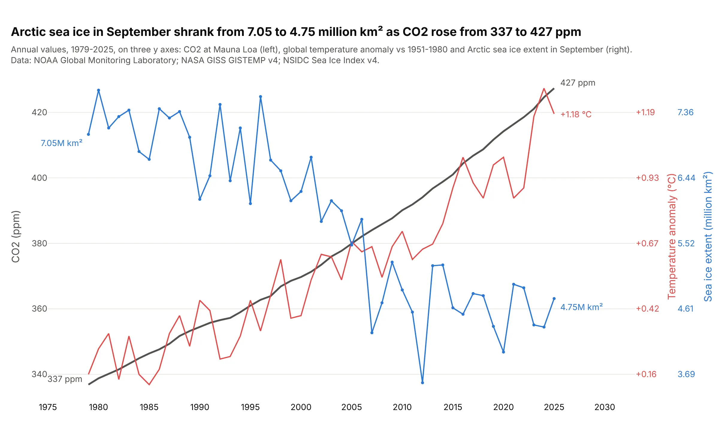
September Arctic sea ice shrank from 7.05 million km² in 1979 to 4.75 million in 2025, while carbon dioxide (CO2) at Mauna Loa rose from 337 to 427 parts per million (ppm). Plotly can add as many y axes as you need; past two, label each line at its ends so readers don't have to match colors to axes. Data: NOAA Global Monitoring Laboratory (GML), NASA GISS GISTEMP v4, National Snow and Ice Data Center (NSIDC) Sea Ice Index v4.

Tip: give the third axis anchor="free" and autoshift=True so Plotly moves it clear of the second.

6. A Pareto chart of US natural gas production

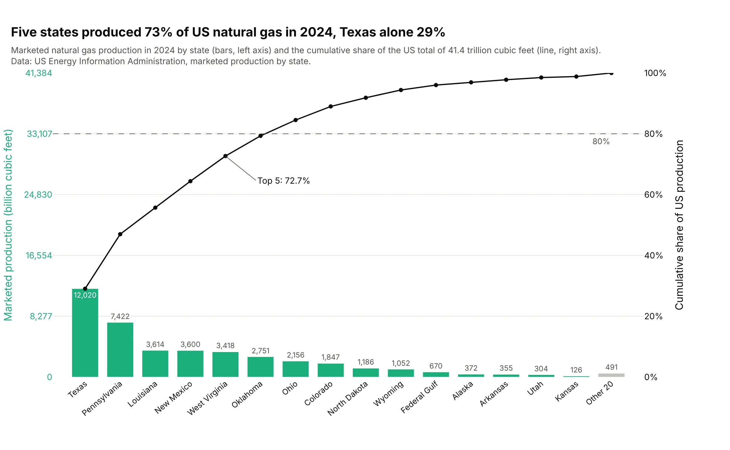
Five states produced 72.7% of US marketed natural gas in 2024, and Texas alone 29%. A Pareto chart is a combo chart whose second axis is the running share of the total, and the Pareto chart guide covers it in depth. Data: US Energy Information Administration, marketed production by state.

Tip: in a Pareto chart the left axis often runs from 0 to the total so each gridline is 20% on both axes; that's the chart's convention rather than a requirement.

7. Walter-Lieth climate diagrams for Seattle and Los Angeles

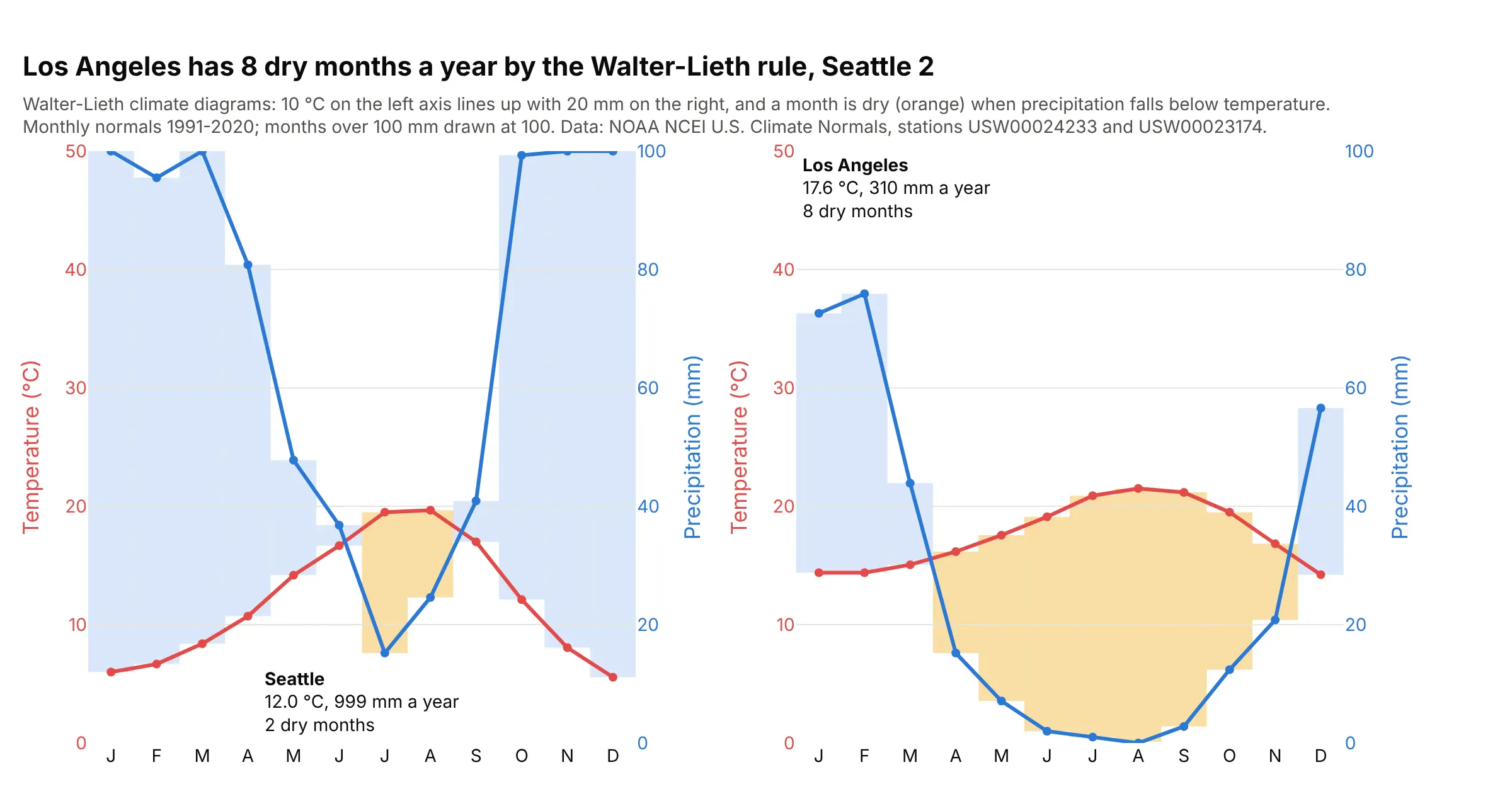
Los Angeles has eight dry months a year by the Walter-Lieth rule and Seattle two. Because 10 °C on the left lines up with 20 mm on the right by convention, the crossings mean something here: a month is dry when the rain line drops below the temperature line. Data: NOAA NCEI U.S. Climate Normals 1991-2020.

Tip: when a convention ties the two scales together, as Walter and Lieth's does, set both ranges from it (0-50 °C and 0-100 mm).

8. A battery test log with voltage, current and temperature

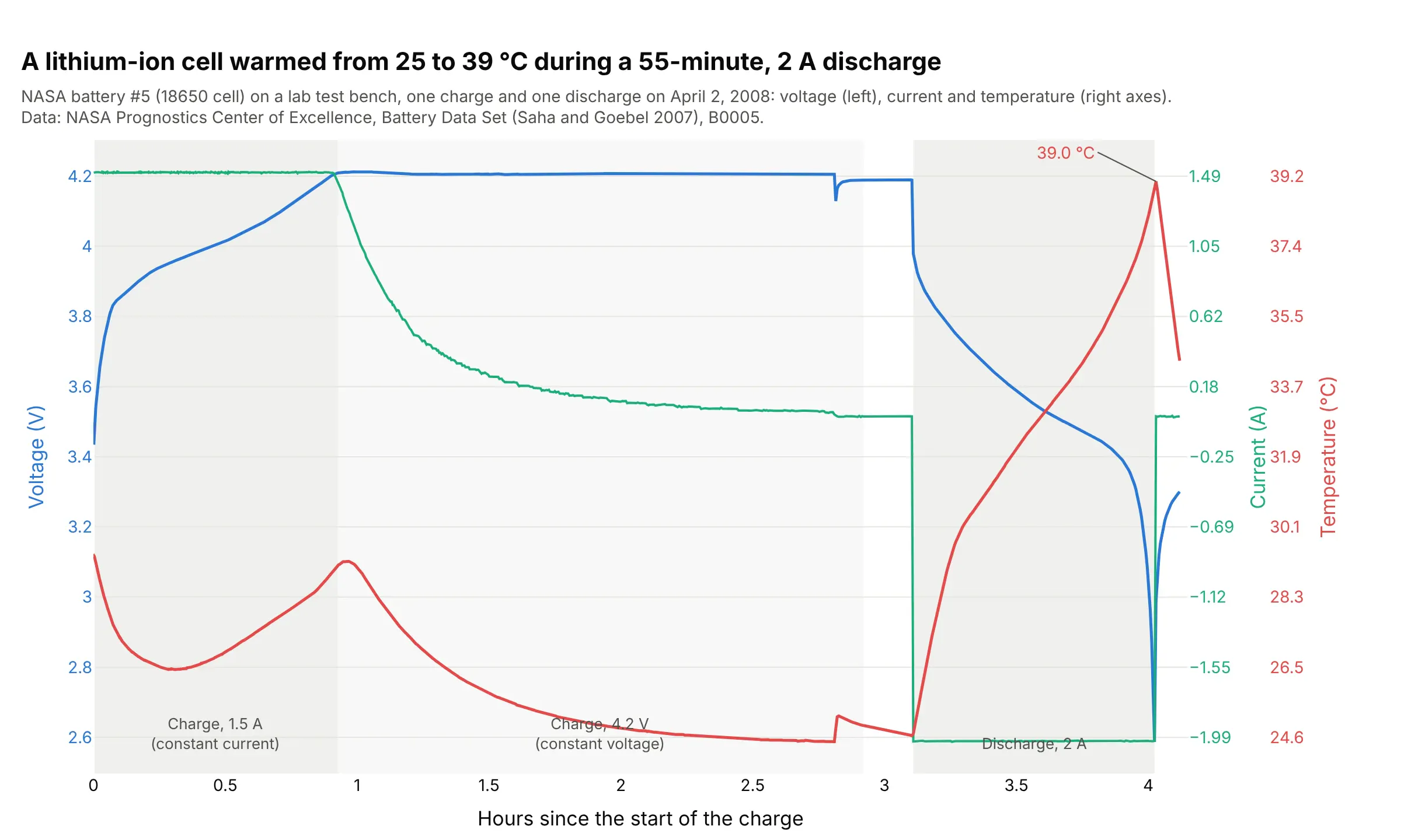
The charger held 1.5 A until the cell reached 4.2 V at 0.93 hours, then held the voltage while the current tapered off. During the 55-minute, 2 A discharge the temperature rose from 24.7 to 39.0 °C, and it peaked 20 seconds after the current stopped. Data: NASA Prognostics Center of Excellence, Battery Data Set (Saha and Goebel 2007), B0005.

Tip: shade the test phases, so readers can match each change in one signal to what the others were doing.

9. Tide height and tidal current in New York Harbor

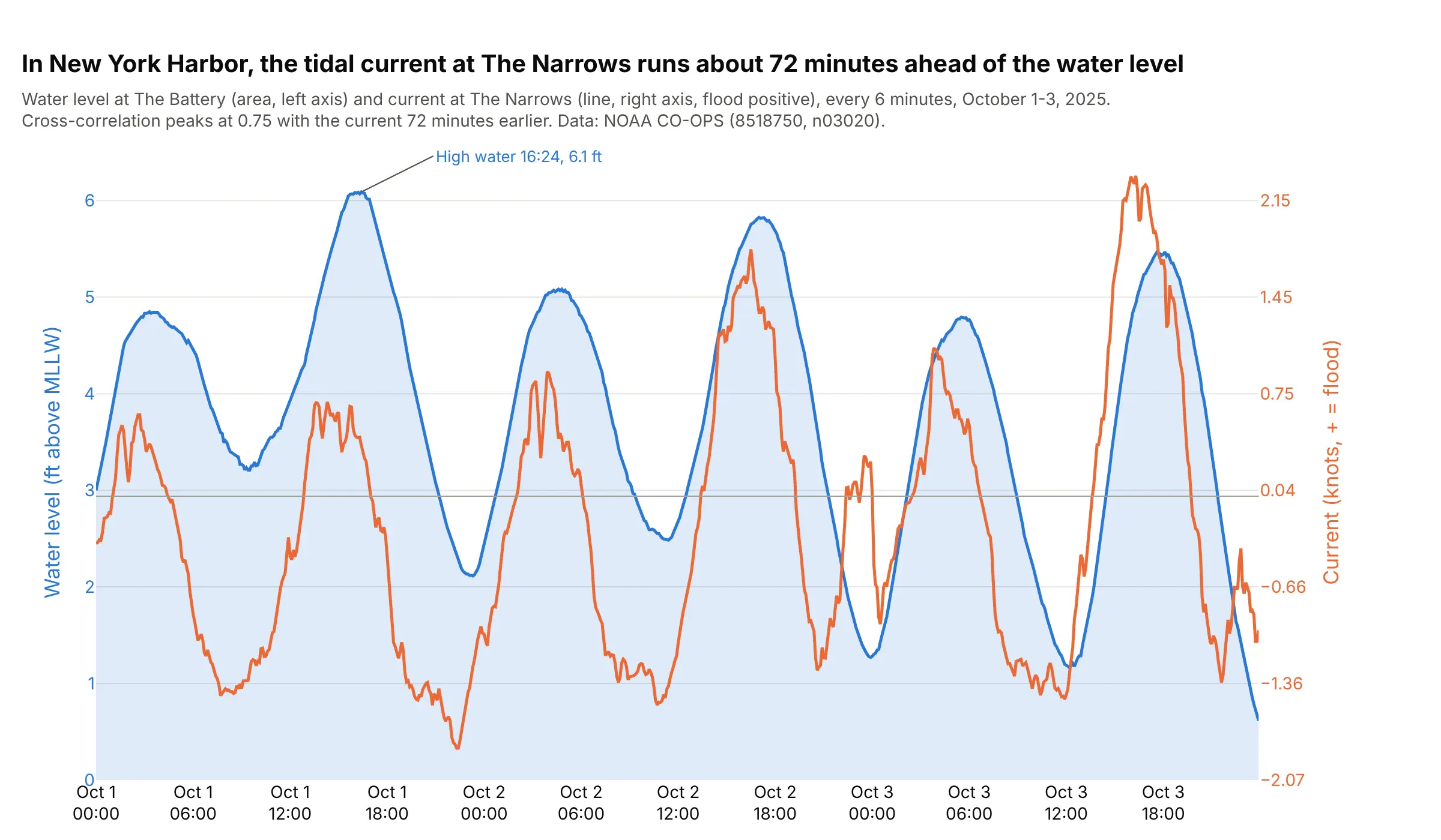
The current at The Narrows peaks about 72 minutes before the water level at The Battery, the lag where the cross-correlation is highest (r = 0.75, against 0.62 with no lag). On one chart you can see each flood current arrive before the high water it brings. Data: NOAA Center for Operational Oceanographic Products and Services (CO-OPS), stations 8518750 (The Battery) and n03020 (The Narrows).

Tip: turn a current's speed and direction into one signed value along its main axis (flood positive), so it can share a chart with the water level.

10. Texas electricity demand and the afternoon heat

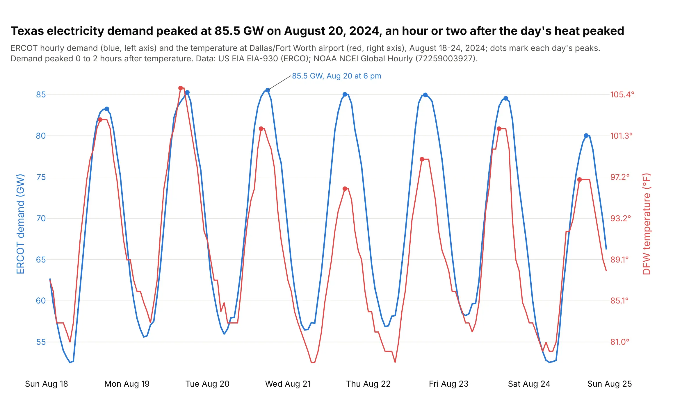
Texas electricity demand peaked at 85.5 GW in the hour ending 6 pm on August 20, 2024, and on six of the seven days demand peaked one or two hours after the temperature at Dallas/Fort Worth did. Data: US EIA Hourly Electric Grid Monitor (Form EIA-930), balancing authority ERCO; NOAA NCEI Global Hourly, station 72259003927 (DFW).

Tip: mark each day's peak on both lines, so the delay between them is visible without a ruler.