
Chris Parmer
2026-11-03
Python Maps - A Complete Guide (with 13 Examples)
TL;DR
- You can make every common kind of map in Python. This guide has 13 of them, each built from real public data, with the libraries it uses and a prompt that rebuilds it with a coding agent.
- GeoPandas reads and processes the data (shapefiles, file geodatabases, GeoJSON, ArcGIS feature and image services) and Plotly draws an interactive map from it, often in one line such as px.scatter_map(df, lat="lat", lon="lon").
- Basemaps, boundary files and ArcGIS services all plug into Plotly. For layers too big to send to a browser, serve vector tiles from DuckDB or PostGIS. In our benchmark of 566,902 public oil and gas well records from Oklahoma and Colorado, vector tiles drew every well in 1.7 s, where a Plotly Scattermap took 19.6 s. The maps at scale and vector tiles deep dives cover both.
- Dash turns a map into an app with the equivalents of ArcGIS Dashboards and of Spotfire marking, where selecting points in one chart filters every other chart. Our example app maps all 76,879 offices of FDIC-insured banks in the 50 states and DC, and its filter callbacks take a median of 4 to 6 ms.
This guide shows how to make maps like these in Python, and every one of them comes with its code or a prompt that rebuilds it:
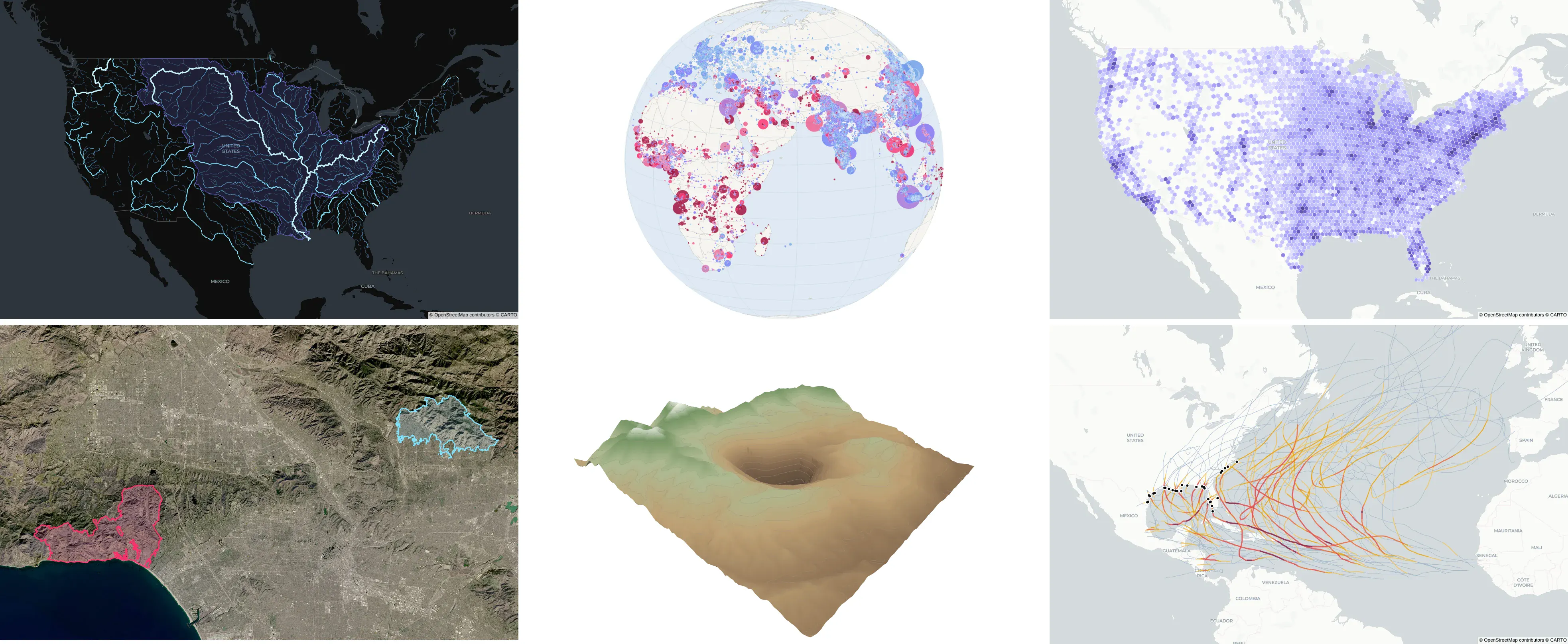
Most people who search for a Python map have a table with coordinates or a file of shapes and want to see it on a map, and teams moving off ArcGIS or Spotfire also want to know where each familiar tool went. This guide starts with 13 example maps from the kind of public data our customers in energy, finance and pharma work with, then covers which library to use, where to get boundaries, basemaps, large maps and vector tiles, Google Maps-style routes, translation tables for ArcGIS and Spotfire, and turning a map into a Dash app.
How to make a map in Python
Install Plotly and GeoPandas with pip install plotly geopandas. A point map needs only a table with latitude and longitude columns. This one draws every earthquake of magnitude 2.5 or more from the last 30 days, straight from the USGS live feed:
Prompt: Read the USGS earthquake feed at https://earthquake.usgs.gov/earthquakes/feed/v1.0/summary/2.5_month.csv with pandas and draw it with px.scatter_map, sized by magnitude, colored by depth, with the place name on hover, on the carto-positron basemap.
import pandas as pdimport plotly.express as pxdf = pd.read_csv("https://earthquake.usgs.gov/earthquakes/feed/v1.0/summary/2.5_month.csv")fig = px.scatter_map(df, lat="latitude", lon="longitude", size="mag", size_max=8,color="depth", hover_name="place", zoom=1, map_style="carto-positron")fig.show()
The 13 examples below build from there, and the sections after them cover your own shapes, basemaps, large maps and apps.
Python map examples
Each example uses real public data and comes with the libraries it uses and a prompt you can give a coding agent to rebuild it. The images are static exports of interactive maps, which zoom, pan and show details on hover.
Points and bubbles
1. Weather stations colored by their 2025 temperature anomaly
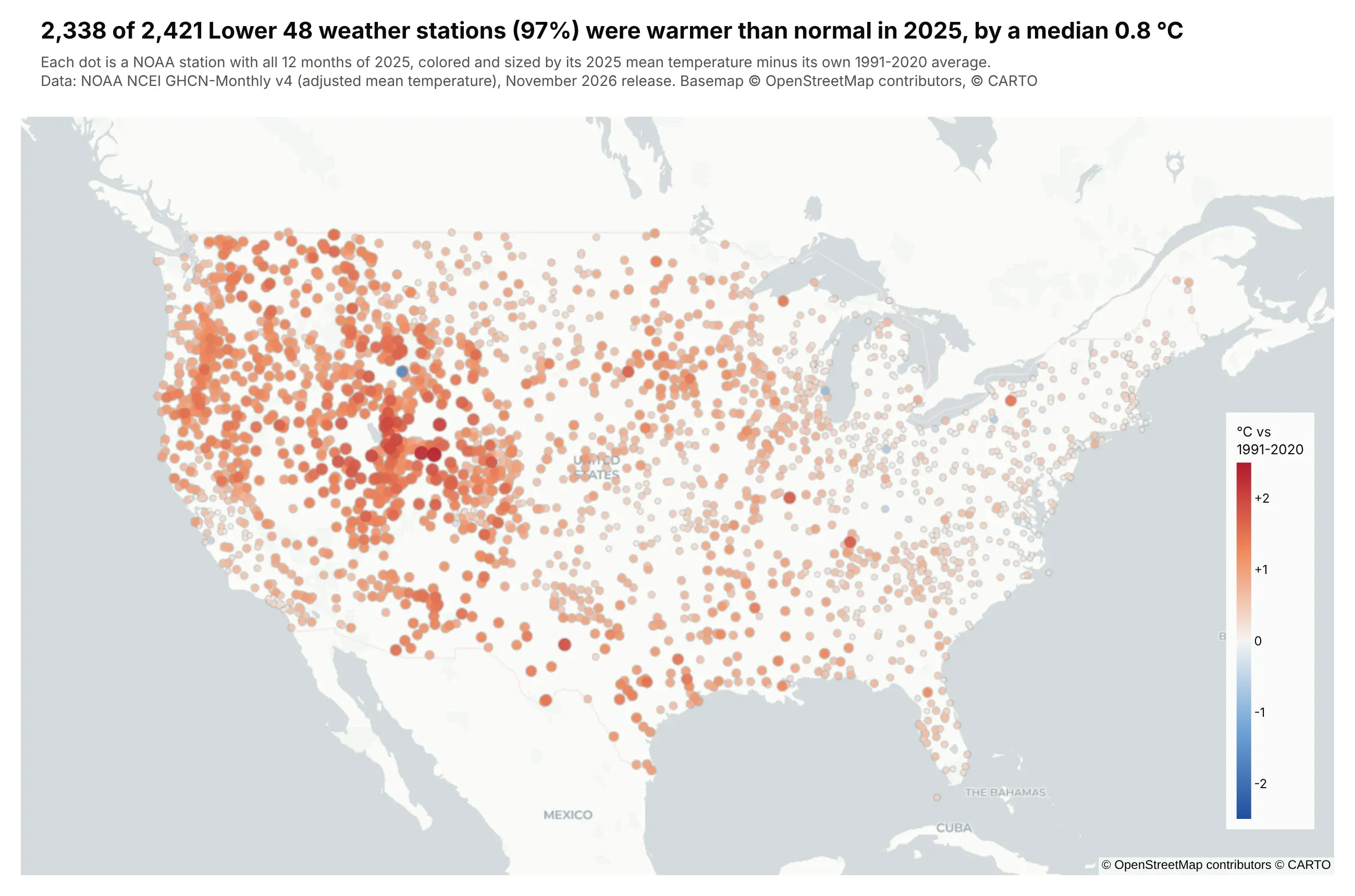
Of the 2,421 NOAA weather stations we mapped in the Lower 48, 2,338 (97%) were warmer in 2025 than their own 1991-2020 average, by a median 0.8 °C. Red means warmer than normal, blue cooler, and bigger dots are further from normal.
Technologies used: Plotly (go.Scattermap), pandas. Data: NOAA NCEI GHCN-Monthly v4, adjusted mean temperature.
Prompt: Download NOAA's GHCN-Monthly v4 adjusted mean temperatures (https://www.ncei.noaa.gov/pub/data/ghcn/v4/ghcnm.tavg.latest.qcf.tar.gz) and parse the station and data files with pandas. For every station in the Lower 48 with all 12 months of 2025 and at least 24 years of each month in 1991-2020, compute its 2025 mean minus its own 1991-2020 average. Map the stations with go.Scattermap on carto-positron, colored on a red-blue scale centered on zero (cmid=0, from -2.5 to +2.5 °C) and sized by how far each is from normal. Title the map with how many stations were warmer than normal.
2. GLP-1 drug trial sites, clustered
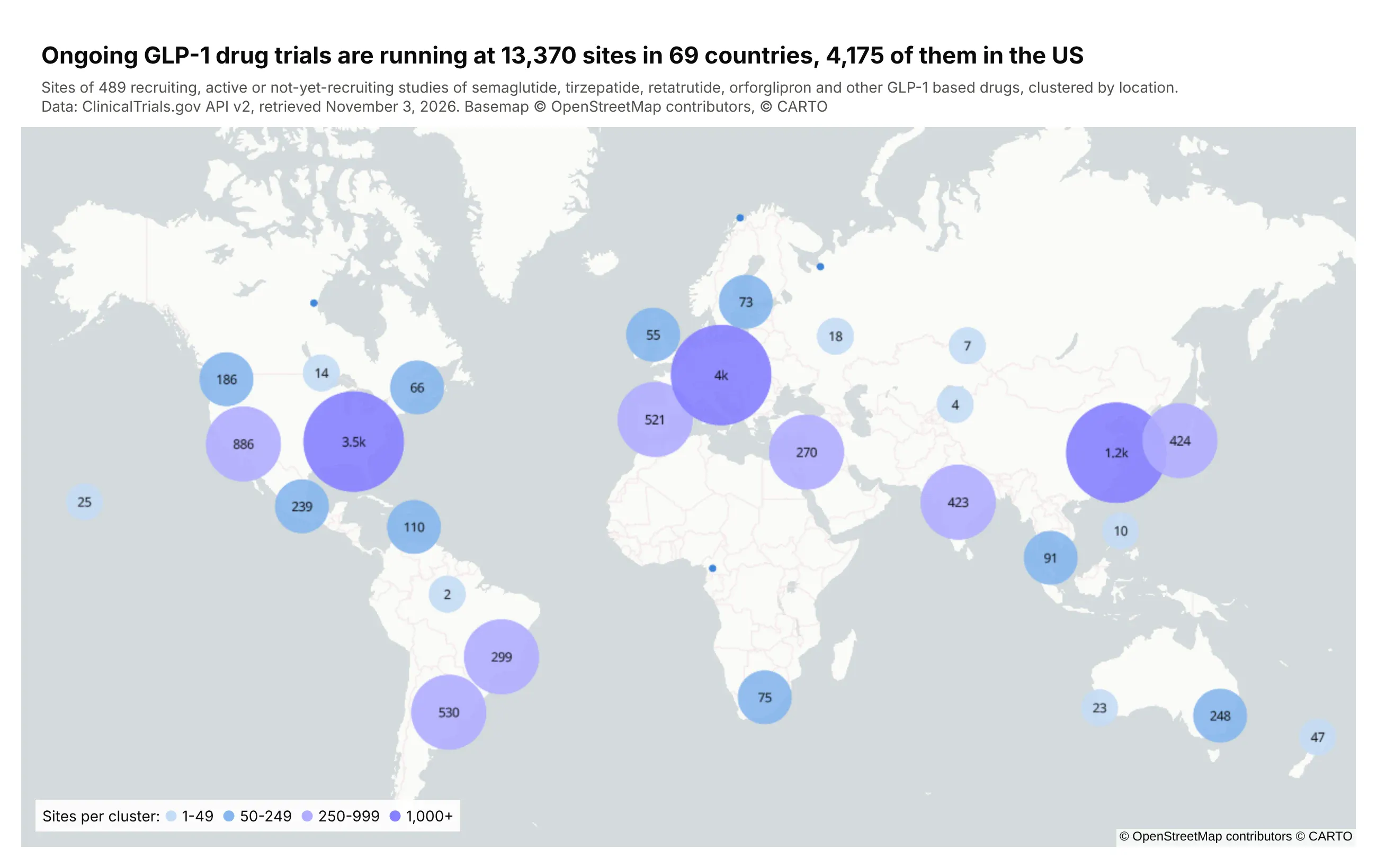
GLP-1 drugs are the diabetes and weight-loss medicines such as semaglutide (Ozempic and Wegovy) and tirzepatide (Mounjaro and Zepbound). Ongoing trials of them are running at 13,370 sites in 69 countries, 4,175 of them in the US. Each circle shows how many sites it holds, and the circles split apart as you zoom in.
Technologies used: Plotly (go.Scattermap with clustering), requests, pandas. Data: ClinicalTrials.gov API v2.
Prompt: Query the ClinicalTrials.gov API v2 (https://clinicaltrials.gov/api/v2/studies) for recruiting, active, not-yet-recruiting and enrolling-by-invitation studies whose interventions include semaglutide, tirzepatide, retatrutide or orforglipron, paging with nextPageToken. Flatten every location that has a geoPoint into one row per site. Draw the sites with go.Scattermap on carto-positron with cluster=dict(enabled=True), using stepped cluster sizes and colors at 50, 250 and 1,000 sites, and add a small key for the steps. Title the map with the number of sites, countries and US sites.
3. The world's cities on a globe, colored by growth since 2000
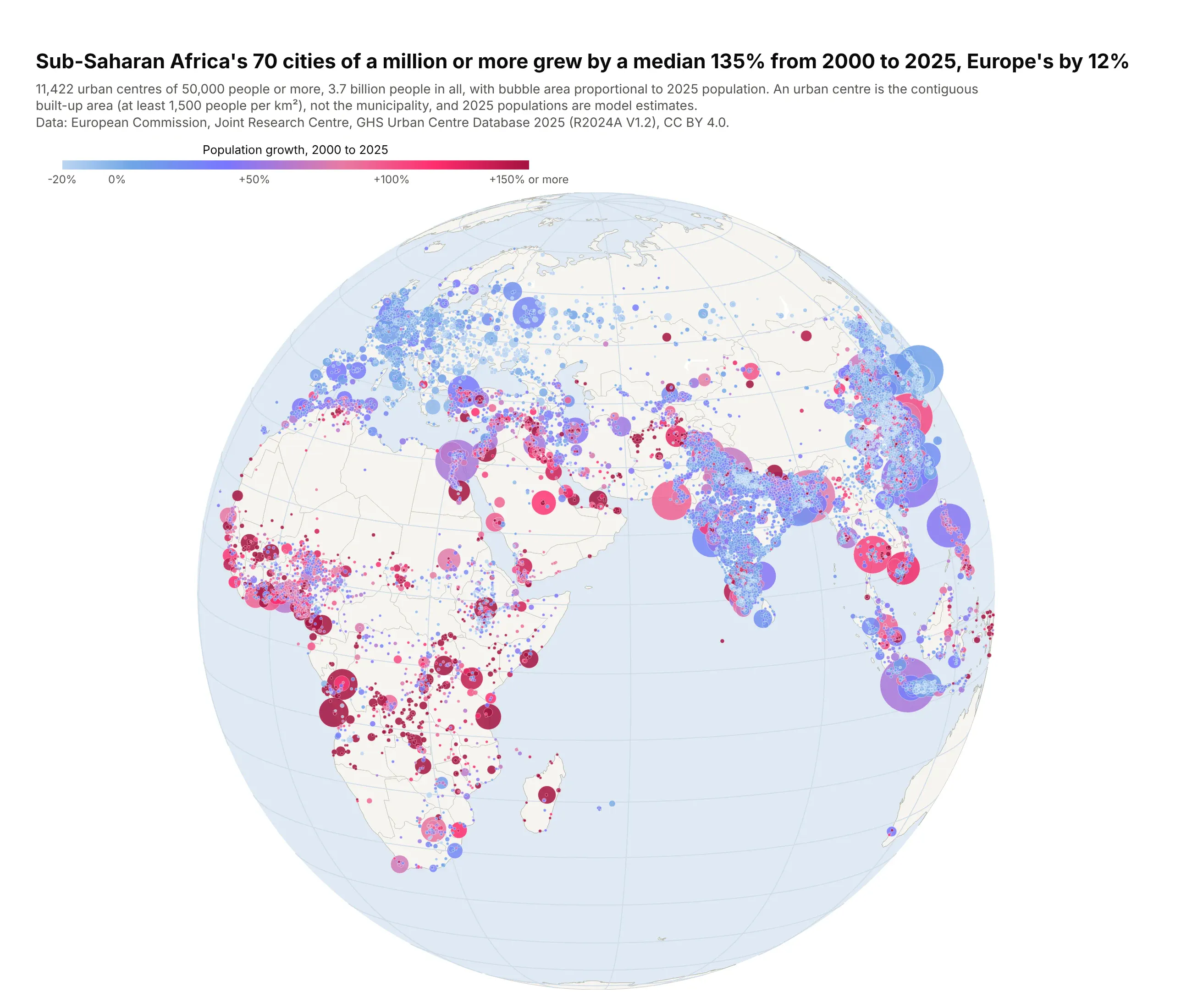
Bubbles are cities sized by their 2025 population and colored by growth since 2000. Sub-Saharan Africa's 70 cities of a million or more grew by a median 135%, Europe's 46 by 12%.
Technologies used: Plotly (go.Scattergeo, orthographic projection), pandas. Data: European Commission JRC, GHS Urban Centre Database 2025 (CC BY 4.0).
Prompt: Download the EU Joint Research Centre's GHS Urban Centre Database 2025 (GHS_UCDB_GLOBE_R2024A_V1_2.zip from the JRC open data site) and read each city's name, region, centroid and its 2000 and 2025 population. Plot the cities with go.Scattergeo on an orthographic projection rotated to longitude 55 and latitude 12, with bubble area proportional to 2025 population and color by percent growth since 2000 on a blue-to-red scale capped at +150%, drawing the largest cities first. Use light land and ocean colors and a horizontal colorbar, and title the map with the median growth of million-plus cities in Sub-Saharan Africa and in Europe.
Lines and routes
4. Rivers of the Lower 48, read from a shapefile
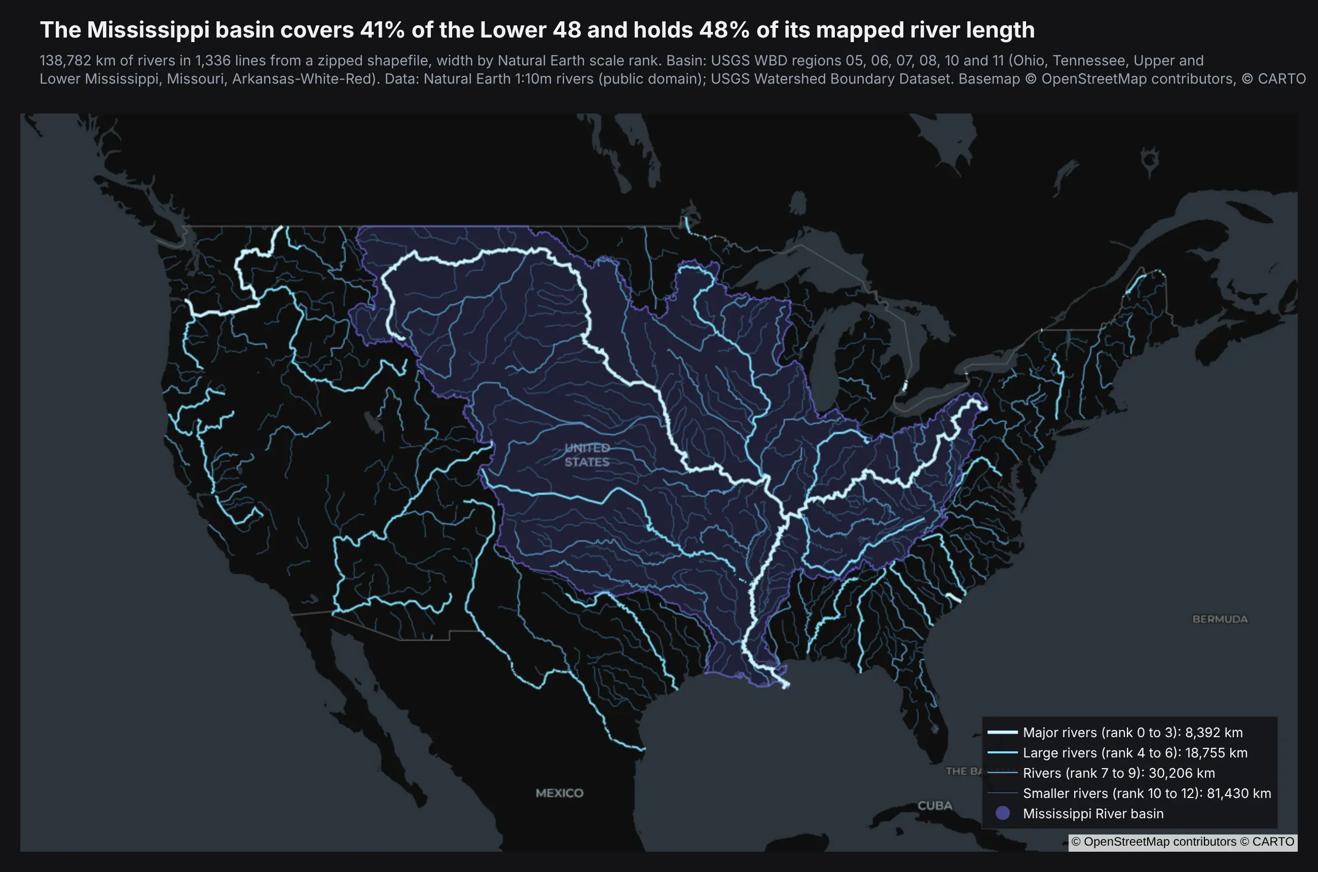
Rivers get wider and brighter as they get bigger. The purple area is the Mississippi basin, which covers 41% of the Lower 48 and holds 48% of its mapped river length.
Technologies used: GeoPandas (read_file, to_crs, clip), pyproj, Plotly (go.Scattermap lines and a MapLibre fill layer). Data: Natural Earth 1:10m rivers (public domain); USGS Watershed Boundary Dataset.
Prompt: Download Natural Earth's 10m rivers_lake_centerlines and North America rivers shapefiles from naciscdn.org and read them with geopandas. Clip them to the Lower 48 using the Census cb_2023_us_state_20m outline, compute each river's length in km with pyproj.Geod, and group the rivers into four size classes by scalerank. Draw each class as one go.Scattermap line trace with the lines joined by None, on carto-darkmatter, with width and brightness growing with size. Add the Mississippi basin (USGS WBD regions 05, 06, 07, 08, 10 and 11 from hydro.nationalmap.gov) as a translucent fill layer underneath, and title the map with the basin's share of land and of river length.
The core of the code is below. CLASSES lists the four size classes with their label, color and width, and line_arrays is the helper shown in the GeoPandas section further down:
gdf = gpd.read_file("ne_rivers_lower48.zip").to_crs(epsg=4326) # stored in Albers (EPSG:5070)for cls, label, color, width in CLASSES:lon, lat, text = line_arrays(gdf[gdf.cls == cls], "label")fig.add_trace(go.Scattermap(lon=lon, lat=lat, mode="lines", name=label,line=dict(color=color, width=width)))
5. The paths of the 2024 and 2045 total solar eclipses
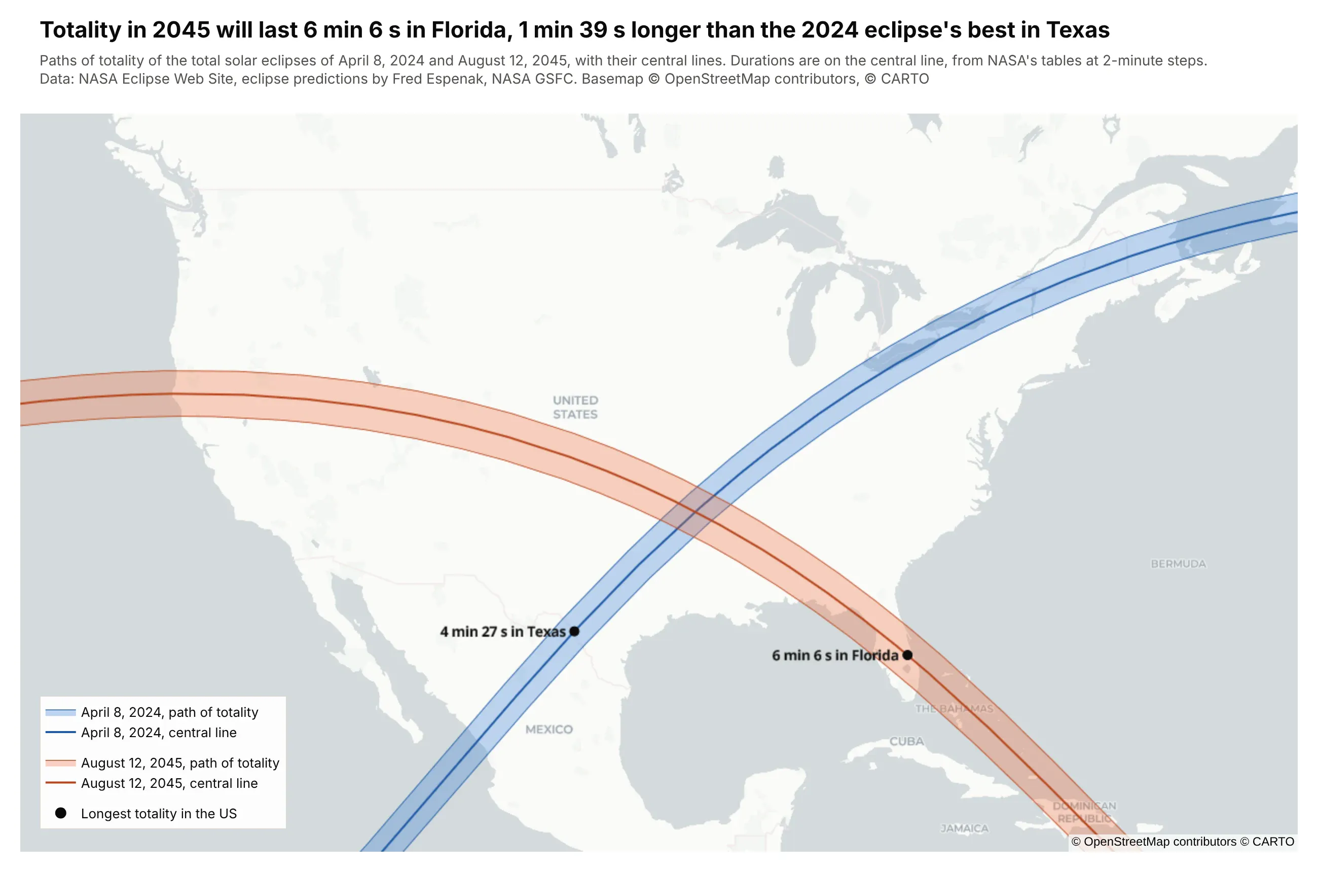
The bands are where totality can be seen, and the line in each band is its center. Totality in 2045 will last 6 min 6 s in Florida, 1 min 39 s longer than the 2024 eclipse's longest point in the US.
Technologies used: Plotly (go.Scattermap with fill="toself"), pandas. Data: NASA Eclipse Web Site path tables (Fred Espenak, NASA GSFC).
Prompt: Parse NASA's eclipse path tables for April 8, 2024 and August 12, 2045 (https://eclipse.gsfc.nasa.gov/SEpath/SEpath2001/SE2024Apr08Tpath.html and SE2045Aug12Tpath.html) with pandas: the northern limit, southern limit and central line every 2 minutes, with the duration of totality. Draw each path as one polygon, up the northern limit and back down the southern, with go.Scattermap and fill="toself", put the central line on top, and label the point with the longest totality inside the US. Use carto-positron, blue for 2024 and orange for 2045, and title the map with the two longest durations.
6. Ten years of Atlantic hurricane tracks, colored by category
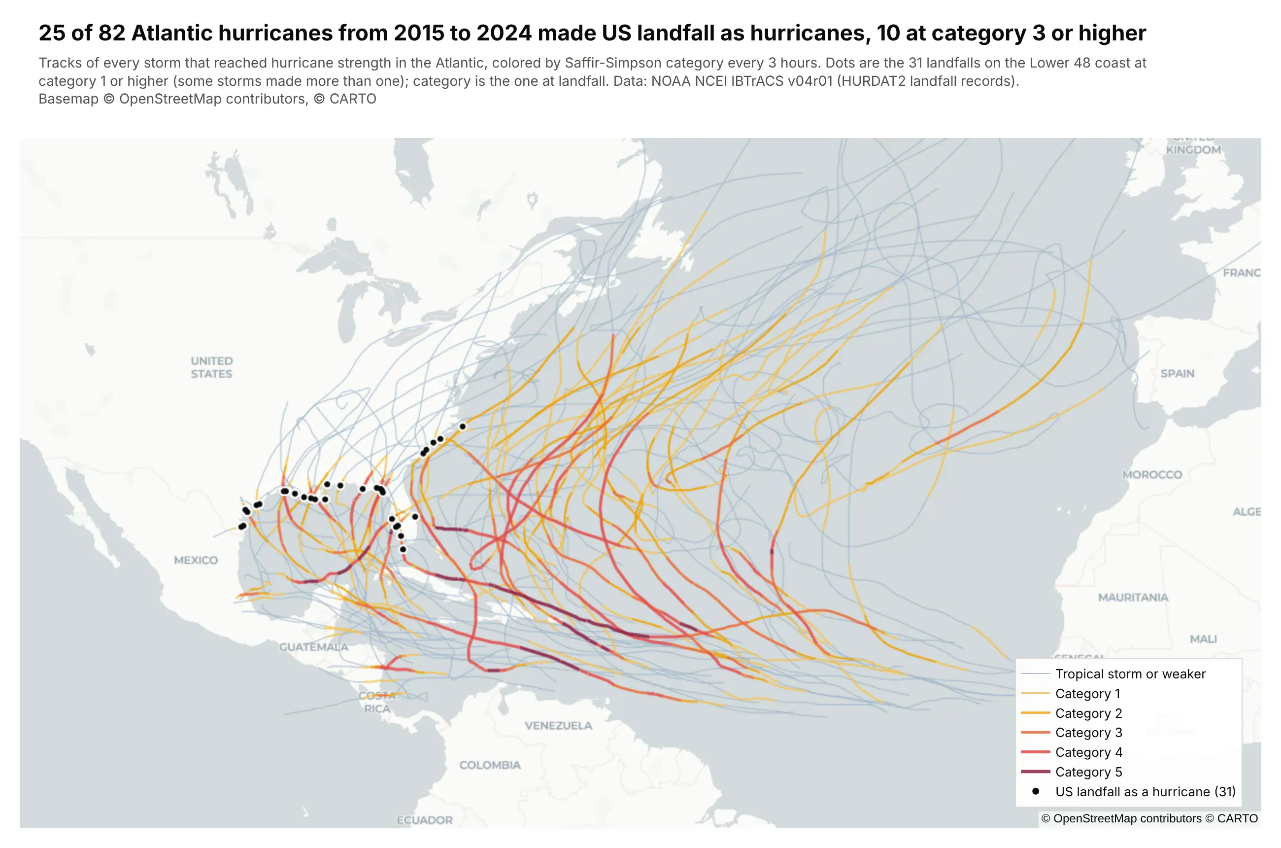
Each track changes color as the storm strengthens or weakens, and the black dots are US landfalls. 25 of the 82 Atlantic hurricanes from 2015 to 2024 hit the US as hurricanes, 10 of them at category 3 or higher.
Technologies used: Plotly (go.Scattermap lines), pandas. Data: NOAA NCEI IBTrACS v04r01, North Atlantic.
Prompt: Download NOAA's IBTrACS North Atlantic CSV (ibtracs.NA.list.v04r01.csv from ncei.noaa.gov) and keep the storms from 2015 to 2024 that reached hurricane strength. Cut every track into 3-hour segments, give each segment its Saffir-Simpson category from USA_SSHS, and draw one go.Scattermap line trace per category so the legend is the color key, from pale blue to dark red. Mark US landfalls (landfall records at category 1 or higher on the Lower 48 coast) as black dots, and title the map with how many hurricanes made US landfall.
Areas and regions
7. Wind and solar's share of electricity, by country
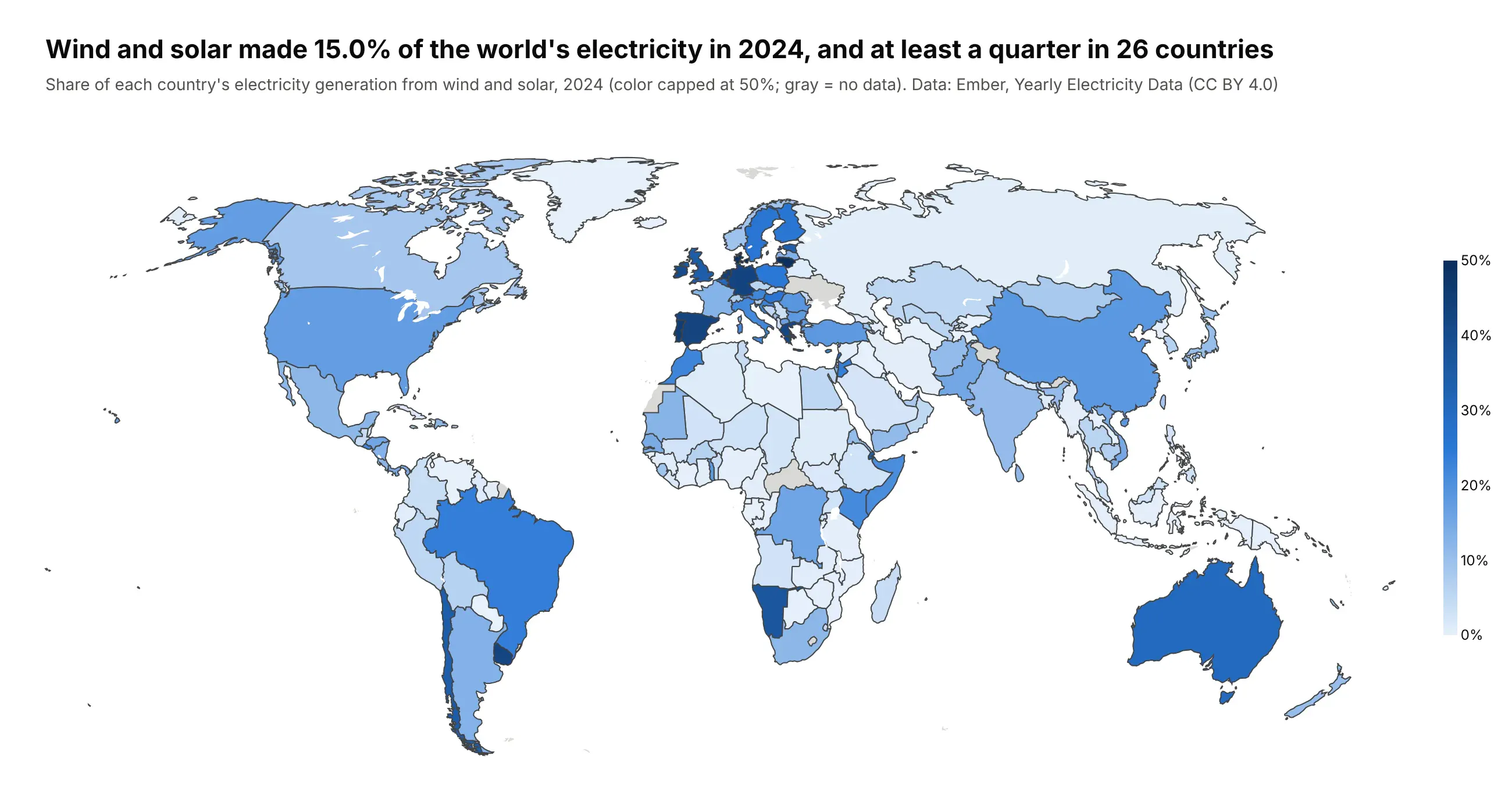
Wind and solar made 15.0% of the world's electricity in 2024, and at least a quarter in 26 countries. Gray countries have no data.
Technologies used: Plotly Express (px.choropleth), pandas. Data: Ember, Yearly Electricity Data (CC BY 4.0).
Prompt: Download Ember's yearly electricity data (release_generation_yearly_global.csv from files.ember-energy.org), keep 2024, and compute wind plus solar as a share of each country's generation. Draw a px.choropleth by ISO-3 code on a natural earth projection with a light-to-dark blue scale capped at 50%, gray for countries without data and Antarctica cropped off. Title the map with the world share and the number of countries at 25% or more.
8. GLP-1 trial sites per million residents, by county
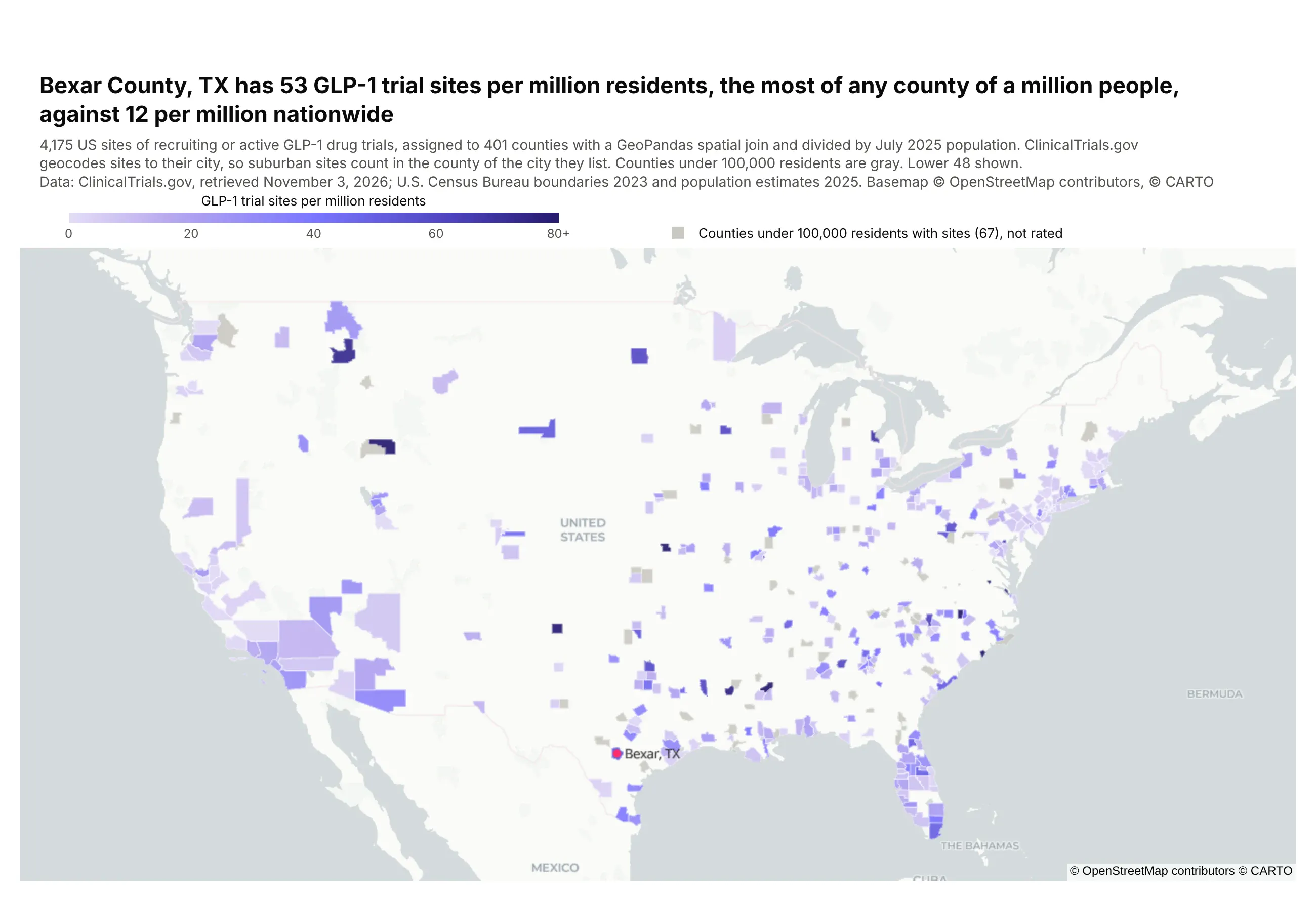
Shading is trial sites per million residents in counties of 100,000 people or more, and gray counties have sites but too few people to rate. Bexar County (San Antonio) leads the counties of a million or more with 53, against 12 nationwide.
Technologies used: GeoPandas (sjoin, sjoin_nearest), Plotly (go.Choroplethmap). Data: ClinicalTrials.gov API v2; U.S. Census Bureau boundaries and 2025 population estimates.
Prompt: Take the US GLP-1 trial sites from example 2, turn them into a GeoDataFrame, and spatially join them into Census counties (cb_2023_us_county_20m.zip) with gpd.sjoin, falling back to gpd.sjoin_nearest for points just offshore. Divide each county's site count by its Census 2025 population estimate (co-est2025-alldata.csv) to get sites per million. Shade counties of 100,000 people or more on a purple scale with go.Choroplethmap, show smaller counties in gray, and title the map with the highest rate among counties of a million people.
The core of the code is below, where df has one row per trial site with its lat and lon, and pop has each county's GEOID and 2025 population:
counties = gpd.read_file("cb_2023_us_county_20m.zip") # NAD83sites = gpd.GeoDataFrame(df, geometry=gpd.points_from_xy(df.lon, df.lat), crs=4326)joined = gpd.sjoin(sites.to_crs(counties.crs), counties, predicate="within")rate = joined.groupby("GEOID").size().div(pop.set_index("GEOID").pop2025).mul(1e6).dropna().reset_index(name="per_m")fig = go.Figure(go.Choroplethmap(geojson=counties.to_crs(4326).__geo_interface__,featureidkey="properties.GEOID", locations=rate.GEOID, z=rate.per_m))
9. Bank branches in H3 hexagons
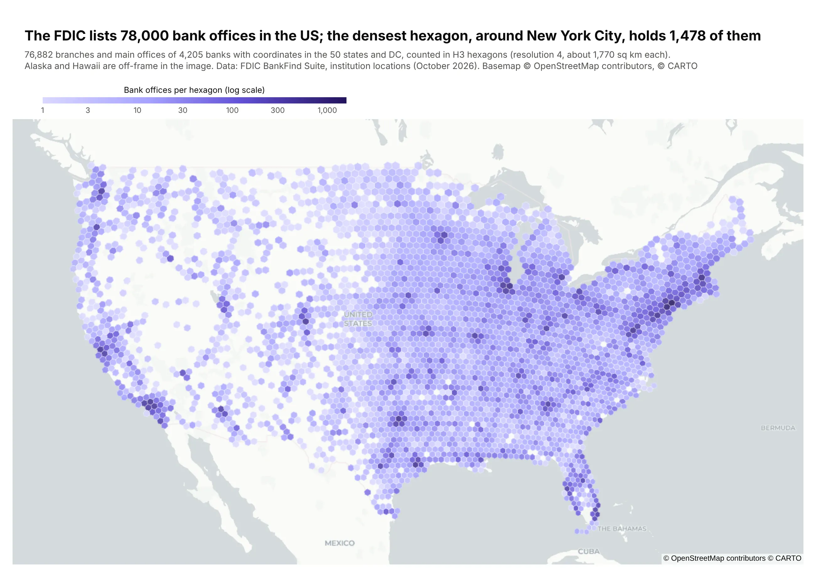
H3 is a grid of hexagons that covers the whole globe, from Uber's open-source h3 library, and counting points per hexagon gives every cell the same area. Each hexagon here covers about 1,770 square km, and darker means more bank offices, on a log scale. The densest, around New York City, holds 1,478 of the 76,882 FDIC-insured bank offices we mapped in the 50 states and DC.
Technologies used: h3, pandas, Plotly (go.Choroplethmap). Data: FDIC BankFind Suite, institution locations.
Prompt: Page through the FDIC BankFind locations API (https://api.fdic.gov/banks/locations, 10,000 rows at a time) to get the latitude and longitude of every bank office. Give each office an H3 cell at resolution 4 with h3.latlng_to_cell, count the offices per cell, and build a GeoJSON of the cells from h3.cell_to_boundary. Draw it with go.Choroplethmap on carto-positron, colored by log10 of the count with colorbar ticks labeled in real counts, and title the map with the total and the densest hexagon.
Density
10. Tornado activity has moved from the Plains toward the Southeast
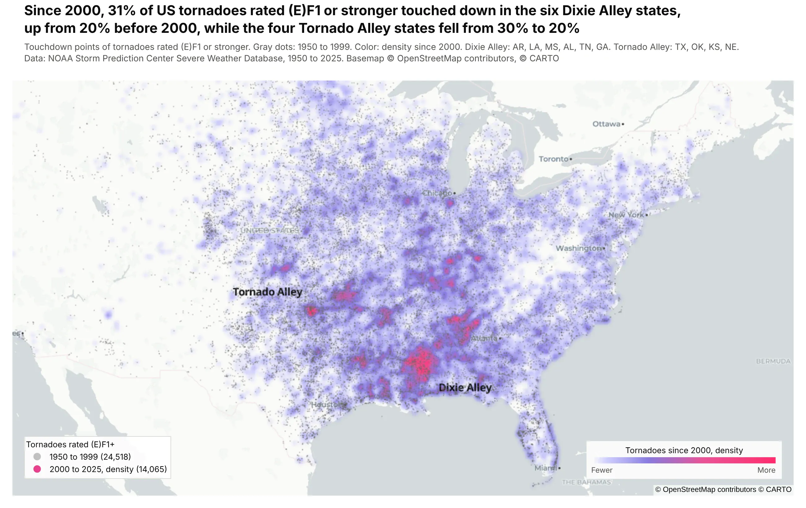
Gray dots are tornadoes rated EF1 or stronger from 1950 to 1999, and the color shows where they've touched down since 2000. The Southeast's share rose from 20% to 31%, while the Plains states fell from 30% to 20%.
Technologies used: Plotly (go.Densitymap, go.Scattermap), pandas. Data: NOAA Storm Prediction Center Severe Weather Database, 1950 to 2025.
Prompt: Download NOAA SPC's tornado database (1950-2025_actual_tornadoes.csv from spc.noaa.gov/wcm), keep tornadoes rated (E)F1 or stronger, and split them at the year 2000. Draw the earlier ones as faint gray go.Scattermap points and the later ones as a go.Densitymap whose colorscale starts fully transparent, on carto-positron. Compute each period's share of tornadoes in Dixie Alley (AR, LA, MS, AL, TN, GA) and Tornado Alley (TX, OK, KS, NE), and put the change in the title.
Imagery and terrain
11. The Palisades and Eaton fire perimeters, on Landsat imagery
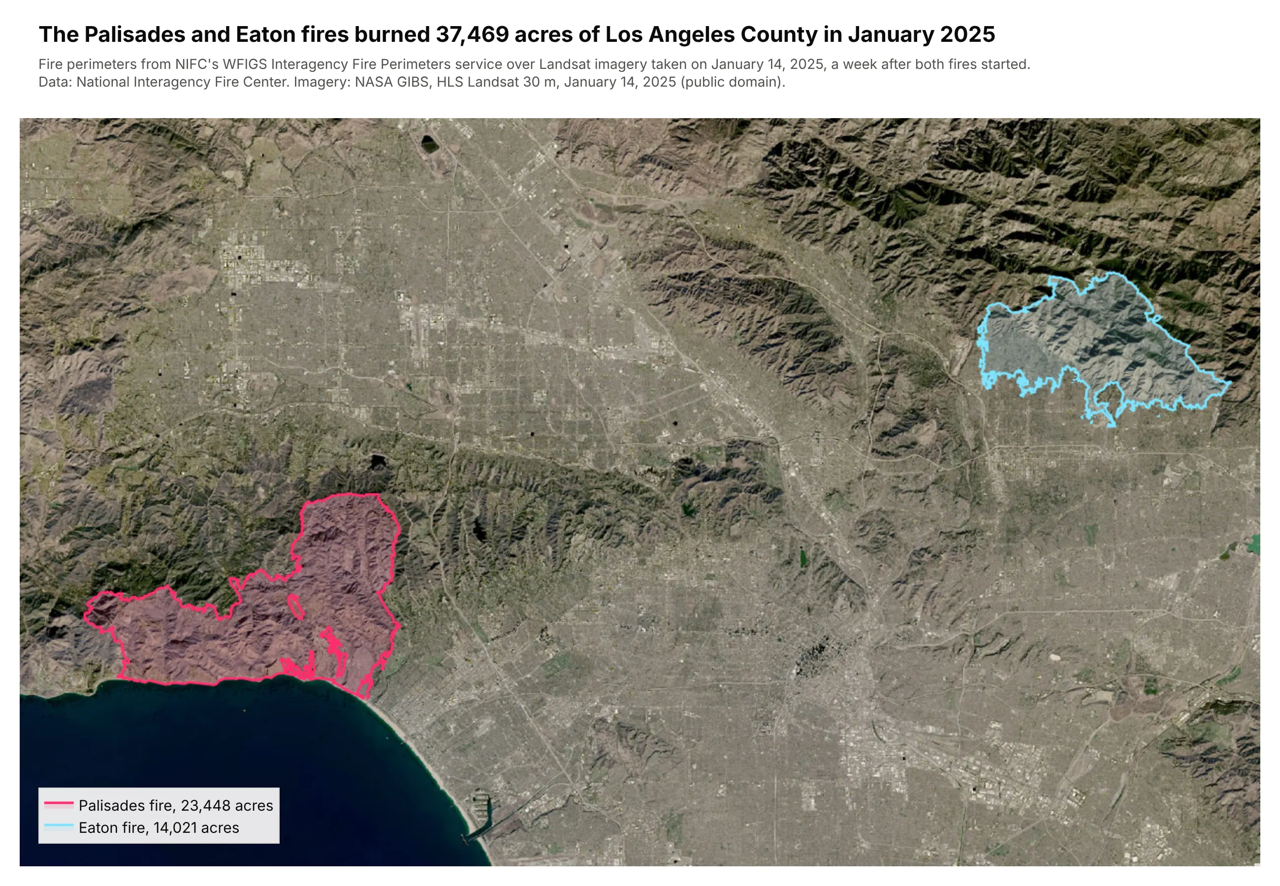
The pink and cyan outlines are the Palisades and Eaton fire perimeters, which burned 37,469 acres together, over Landsat imagery from a week after the fires started.
Technologies used: requests, Plotly (go.Scattermap, an image layer in map.layers). Data: NIFC WFIGS Interagency Fire Perimeters (ArcGIS feature service); NASA GIBS, Harmonized Landsat Sentinel-2 imagery.
Prompt: Query NIFC's WFIGS Interagency Perimeters feature service for the 2025 Palisades and Eaton fires with f=geojson and outSR=4326, and read each fire's acreage. Download NASA GIBS HLS_L30 true-color tiles for January 14, 2025 over Los Angeles, stitch them into one image, and add it to a Plotly map with map.layers sourcetype="image" and the image's corner coordinates. Draw each perimeter as a go.Scattermap outline with a translucent fill, and title the map with the total acres burned.
12. Bingham Canyon mine in 3D, from a USGS ArcGIS ImageServer
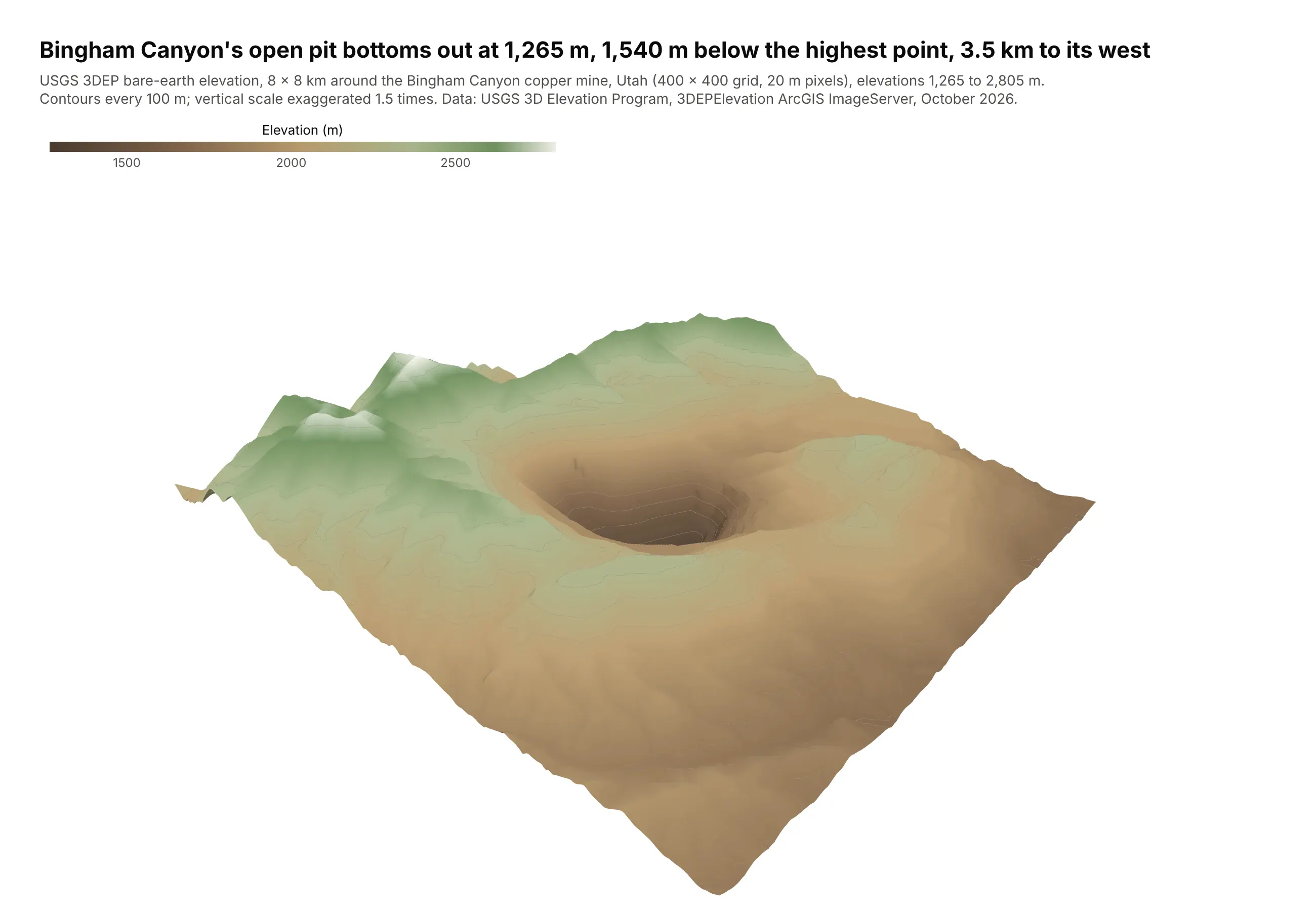
Color is elevation, with contours every 100 m and the vertical scale exaggerated 1.5 times. The open pit bottoms out at 1,265 m, 1,540 m below the highest point in the 8 by 8 km box.
Technologies used: requests, tifffile, NumPy, Plotly (go.Surface). Data: USGS 3D Elevation Program, 3DEPElevation ImageServer.
Prompt: Request an 8 by 8 km box around the Bingham Canyon mine in Utah from the USGS 3DEP ImageServer's exportImage endpoint (bboxSR and imageSR 26912, size 400,400, format tiff, pixelType F32), read it into NumPy with tifffile and flip the rows so row 0 is south. Draw it with go.Surface in an earth-tone colorscale with contours every 100 m, a camera looking into the pit and a 1.5x vertical exaggeration set with aspectratio, and title it with the pit's depth below the highest point.
The core of the request is below, where x0, y0, x1, y1 are the corners of the box in UTM zone 12N meters (EPSG:26912) and EARTH is the colorscale:
params = {"bbox": f"{x0},{y0},{x1},{y1}", "bboxSR": 26912, "imageSR": 26912, "size": "400,400","format": "tiff", "pixelType": "F32", "f": "image"}r = requests.get(".../3DEPElevation/ImageServer/exportImage", params=params)z = np.flipud(tifffile.imread(io.BytesIO(r.content)))fig = go.Figure(go.Surface(z=z, colorscale=EARTH, contours_z=dict(show=True, start=1300, end=2800, size=100)))
Change over time
13. Oklahoma's earthquakes, year by year
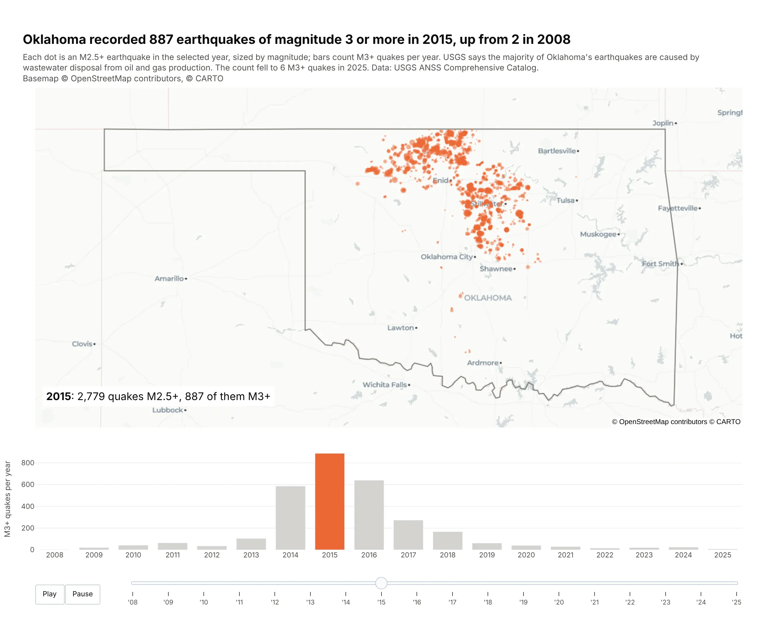
Dots are 2015's earthquakes of magnitude 2.5 or more, and the bars count magnitude 3 or more per year, from 2 in 2008 to 887 in 2015 and 6 in 2025. The play button animates both. The USGS says most of Oklahoma's earthquakes are caused by wastewater disposal from oil and gas production.
Technologies used: Plotly (make_subplots, go.Scattermap, go.Bar, animation frames), pandas. Data: USGS ANSS Comprehensive Catalog.
Prompt: Query the USGS earthquake catalog (earthquake.usgs.gov/fdsnws/event/1/query with format=csv) for magnitude 2.5 or larger events in a box around Oklahoma from 2008 to 2025, and keep those inside the Census state outline. Build one figure with make_subplots: a go.Scattermap of each year's earthquakes sized by magnitude above a bar chart of magnitude 3 or larger earthquakes per year. Add animation frames that update the map and highlight the current year's bar, play and pause buttons and a year slider, start on 2015, and title the figure with the 2008 and 2015 counts.
Types of maps you can make in Python
Plotly has two families of map traces. Tile maps (scatter_map, line_map, choropleth_map, density_map) draw on a zoomable web basemap of streets, a dark background or satellite imagery, and suit anything you want to explore from the country level down to a single street. Outline maps (scatter_geo, line_geo, choropleth) draw countries and coastlines in a map projection such as Robinson, Albers or an orthographic globe, with no tiles, which suits world and national maps that will be printed or put in a report.
- Point or bubble map (px.scatter_map, go.Scattermap) for locations sized or colored by a value. Example 1, weather stations.
- Clustered points (go.Scattermap(cluster=...)) for thousands of points that pile up on the same places. Example 2, GLP-1 trial sites.
- Globe (go.Scattergeo with projection_type="orthographic") for world data with a 3D feel and no tiles. Example 3, world cities.
- Line map (go.Scattermap(mode="lines"), px.line_map) for rivers, routes, tracks and paths. Examples 4 to 6, rivers, eclipse paths and hurricanes.
- Choropleth (px.choropleth, px.choropleth_map) for a rate or share per region. Examples 7 and 8, wind and solar by country and trial sites by county.
- Hexbin map (go.Choroplethmap on H3 hexagons) for point counts in equal-area cells. Example 9, bank branches.
- Density heat map (px.density_map, go.Densitymap) for where points concentrate. Example 10, tornadoes.
- Satellite or imagery map (any trace plus a raster tile layer) for physical context such as coastlines, land cover and burn scars. Example 11, wildfires in Los Angeles.
- 3D terrain (go.Surface on an elevation grid) for elevation and relief. Example 12, the Bingham Canyon mine.
- Animated map (animation_frame= or frames) for change over time. Example 13, Oklahoma earthquakes.
- Vector tile map (a MapLibre style with a vector source) for layers too big to send to the browser at once. See the vector tiles section.
- Route map (a street network from OSMnx, a path-finding library and go.Scattermap lines on a street basemap) for Google Maps-style directions and drive times. See the route map section.
- Map app (Dash) for filters, selection and linked charts around a map. See the Dash section.
For the choropleth map specifically (classing, color scales, county and custom GeoJSON boundaries), our Choropleth Maps guide goes deeper, with 14 more examples.
Which Python library should you use to make a map?
Most Python mapping work splits into two jobs. One library reads, reprojects and joins the geographic data, and another one draws it. For the first job the standard is GeoPandas, which reads shapefiles, file geodatabases, GeoPackages and GeoJSON into a table with a geometry column and runs the spatial operations a GIS analyst expects (spatial joins, buffers, dissolves, clips and reprojection). For drawing, the main choices are:
Library
What it draws
Good for
Watch out for
Plotly (plotly.express, plotly.graph_objects)
Interactive tile maps on street, dark or satellite basemaps (MapLibre), and outline maps with map projections
Points, lines, choropleths, density, animation and 3D terrain with one API, and maps inside Dash apps
Tile maps need coordinates in longitude and latitude (EPSG:4326)
Web apps around Plotly maps
Map explorers with filters, selection, click-to-inspect and linked charts
It's a web framework, so you deploy the app somewhere (Plotly Cloud, Dash Enterprise or your own server)
GeoPandas .plot()
Static matplotlib maps
A quick look at a layer while you work
No zooming or hovering, and styling takes a lot of matplotlib code
Leaflet.js web maps
Simple marker and GeoJSON maps saved as HTML
Leaflet draws features as SVG by default, so maps with tens of thousands of features get slow
pydeck and kepler.gl
deck.gl WebGL layers
Large point clouds and 3D extrusions
Separate APIs from the rest of your charts
Static matplotlib maps with many projections
Publication figures in climate and earth science
Static only
Esri web maps in notebooks
Managing content in an ArcGIS Online or ArcGIS Enterprise organization
Most features need an ArcGIS account
We recommend GeoPandas for the data and Plotly for the maps, then Dash when the map needs to become an app other people use, and every example in this post is built that way. Plotly draws maps with the same API you already use for line charts and bar charts, so a map can share a page, a hover style and a callback with the rest of an analysis.
For the data side, GeoPandas now has company: DuckDB's spatial extension, the polars-st plugin for Polars, and SedonaDB from the Apache Sedona project all run the same spatial joins and reprojections, often on every CPU core. We timed all of them on public US watersheds, rivers and Overture Maps places in our Python geospatial libraries comparison. SedonaDB counted 10 million points into 87,028 watersheds in 21.5 s, and GeoPandas went from 320 s to 23.3 s on the same job just by running the join from the polygon side, which is a good sign of how much the way you write a query matters.
Map libraries for Dash apps
When the map goes into a Dash app, there are four more options besides Plotly's own map traces, all open source and maintained by the community:
Library
Built on
What it adds
Plotly map traces (Scattermap, Choroplethmap, Densitymap)
MapLibre GL (WebGL)
Hover, click and lasso events, legends, partial updates with Patch(), and crossfiltering with every other Dash component. layout.map.style takes any MapLibre style, so the same map can also draw vector tiles and raster services
Leaflet
Drawing and editing geometry, measuring, WMS layers, a classic layer control and fast marker clustering
deck.gl 9 (WebGL)
GPU layers for millions of points, arcs, 3D columns and heatmaps, with binary data transport. It replaces Plotly's original dash-deck, which hasn't been updated since its 0.0.1 release in 2020 and can't load in the same app
OpenLayers
OGC services, map projections, editing tools and fast vector tile rendering
Leaflet 2
An early look at Leaflet 2 for Dash 4, with pointer events for touch and stylus and map rotation
Which one to use depends mostly on how big the layer is. Our maps at scale deep dive benchmarks all five on the same public layers, 566,902 oil and gas wells from Oklahoma and Colorado and 84,000 census tracts, and explains the data formats (GeoJSON, binary arrays, vector tiles) and rendering engines (SVG, canvas, WebGL) that decide how far each one goes.
Your own shapes and lines: from GeoPandas to Plotly
A world choropleth needs only ISO country codes, because Plotly has country outlines built in. This is the core of example 7 above, with df holding a country code and a value per row:
Prompt: Draw a world choropleth with px.choropleth from a DataFrame with an iso3 country code column and a share_pct value column, using the natural earth projection, the country name on hover and a color range of 0 to 50.
fig = px.choropleth(df, locations="iso3", color="share_pct", hover_name="country",projection="natural earth", range_color=(0, 50))
For your own shapes, read them with GeoPandas and pass the geometry to Plotly. A shapefile, a zipped shapefile, a file geodatabase layer, a GeoPackage and a GeoJSON URL all go through the same read_file call:
Prompt: Read the Census cb_2023_us_county_20m.zip shapefile straight from its URL with GeoPandas, reproject it to EPSG:4326, compute each county's land area in square kilometers from ALAND, and draw it with px.choropleth_map on carto-positron, centered on the US.
import geopandas as gpdimport plotly.express as pxcounties = gpd.read_file("https://www2.census.gov/geo/tiger/GENZ2023/shp/cb_2023_us_county_20m.zip")counties = counties.to_crs(epsg=4326) # tile maps need longitude and latitudecounties["sq_km"] = counties.ALAND / 1e6fig = px.choropleth_map(counties, geojson=counties.geometry, locations=counties.index,color="sq_km", hover_name="NAME", range_color=(0, 5000),map_style="carto-positron", zoom=3, center={"lat": 38, "lon": -96})fig.show()
Lines take one more step, because Plotly draws many lines in one trace from flat longitude and latitude lists with None between the lines. This helper turns any GeoDataFrame of lines into those lists:
Prompt: Write a helper that turns a GeoDataFrame of LineString and MultiLineString geometries into flat lon and lat lists with None between lines, then draw all the lines as one go.Scattermap trace with mode="lines".
def line_arrays(gdf):lon, lat = [], []for geom in gdf.geometry:parts = geom.geoms if geom.geom_type == "MultiLineString" else [geom]for part in parts:xs, ys = part.xylon += list(xs) + [None]lat += list(ys) + [None]return lon, latlon, lat = line_arrays(rivers)fig = go.Figure(go.Scattermap(lon=lon, lat=lat, mode="lines"))
Use one trace per category (one per stream order, say) rather than one per line. Ten thousand traces make the map slow and the legend unusable, while ten traces of a thousand lines each draw quickly.
Where to get GeoJSON for a choropleth map
A choropleth needs two things: your values, and the shapes of the regions they belong to, with an id in both that matches. Finding the shapes is usually the harder part. Plotly has countries and US states built in, and for everything else there's a public source for almost any boundary you'd want. The grid below draws one small choropleth from each of six of them, and the table after it gives the setting that joins the data to the shapes:
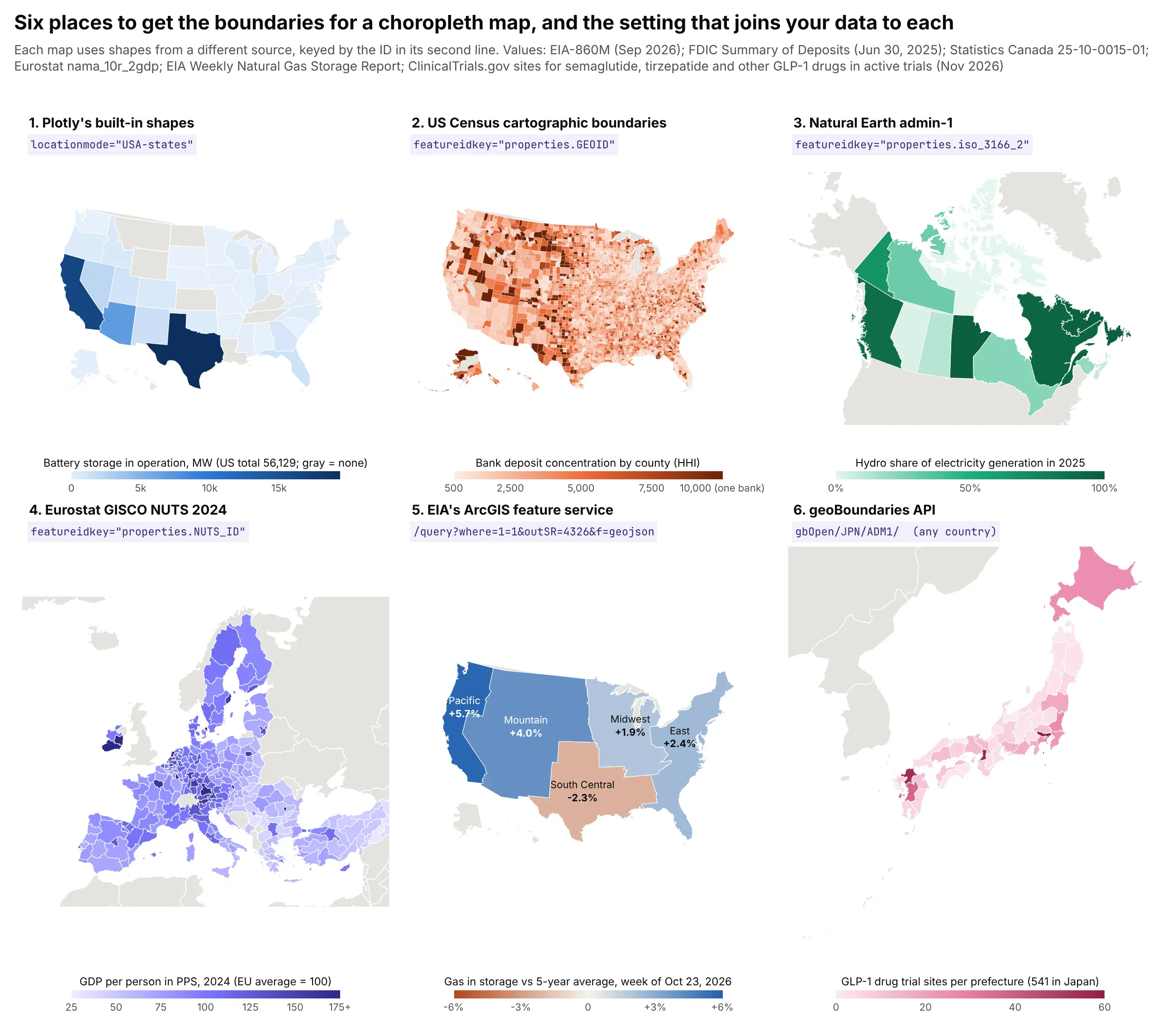
Technologies used: Plotly (make_subplots with geo subplots, go.Choropleth), GeoPandas, requests.
Prompt: Make a 3 by 2 grid of choropleth maps with Plotly make_subplots and geo subplots, each from a different boundary source: Plotly's built-in US states (locationmode="USA-states"), Census cb_2023_us_county_20m counties keyed on properties.GEOID, Natural Earth admin-1 provinces keyed on properties.iso_3166_2, Eurostat GISCO NUTS-2 2024 regions keyed on properties.NUTS_ID, an ArcGIS feature service layer queried with f=geojson and outSR=4326, and geoBoundaries ADM1 boundaries keyed on properties.shapeISO. Give each panel a title naming its source, its featureidkey as a small code label, its own color scale, colorbar, projection and extent.
Source
What it has
How to load it
Join on
Plotly built in
Countries, US states
px.choropleth(df, locations="iso3") or locationmode="USA-states"
ISO-3 code or state abbreviation
States, counties, tracts, ZIP code areas, congressional districts
gpd.read_file(".../cb_2023_us_county_20m.zip")
properties.GEOID (5-digit county FIPS as a string)
Countries, states and provinces worldwide, coastlines, rivers
gpd.read_file(".../ne_10m_admin_1_states_provinces.zip")
properties.iso_3166_2 or adm0_a3
EU NUTS regions at levels 0 to 3, by year
requests.get(".../NUTS_RG_20M_2024_4326_LEVL_2.geojson").json()
properties.NUTS_ID
ArcGIS feature services
Boundaries that only exist in GIS: watersheds, storage regions, management areas, basins
/query?where=1=1&outSR=4326&f=geojson
Whatever id field the layer has
Administrative levels 1 to 5 for almost every country
requests.get(".../api/current/gbOpen/JPN/ADM1/").json()["simplifiedGeometryGeoJSON"]
properties.shapeISO
Your own
H3 hexagons, buffers, Voronoi cells, sales territories
h3.cell_to_boundary, gdf.buffer, gdf.dissolve("territory")
The id you create
The setting that ties it together is featureidkey, which tells Plotly where the id lives in each GeoJSON feature. Your data column goes in locations:
Prompt: Join my county table (a fips column and an hhi value) to the Census cb_2023_us_county_20m counties: read the shapefile with GeoPandas, reproject to EPSG:4326, pad fips to 5 characters with zfill, and draw a go.Choroplethmap with geojson from __geo_interface__ and featureidkey="properties.GEOID".
counties = gpd.read_file("https://www2.census.gov/geo/tiger/GENZ2023/shp/cb_2023_us_county_20m.zip")counties = counties.to_crs(4326)df["fips"] = df["fips"].astype(str).str.zfill(5) # 1001 -> "01001"fig = go.Figure(go.Choroplethmap(geojson=counties.__geo_interface__, featureidkey="properties.GEOID",locations=df.fips, z=df.hhi))
A few things to check when you bring in shapes from somewhere new:
- Codes stored as numbers lose their leading zeros. FIPS codes and ZIP codes are strings. Read them with dtype=str or pad them with str.zfill, otherwise every state from Alabama to Connecticut silently goes blank.
- Boundaries change, so match the year. Connecticut replaced its 8 counties with 9 planning regions in the 2022 Census files, and Eurostat's NUTS codes change between the 2016, 2021 and 2024 versions. Use the boundary year your data was coded with.
- Join on codes, not names. Natural Earth writes "Québec" and Statistics Canada writes "Quebec". Natural Earth also uses "-99" for a few countries' ISO code, so join countries on ADM0_A3 instead.
- Simplify before you draw. The full Natural Earth admin-1 file is 15 MB zipped, and the full geoBoundaries Japan file is 63 MB. gdf.simplify(0.005) and rounding coordinates to 4 decimals took the US county file to 1.3 MB of GeoJSON. For layers that share edges, GeoSeries.simplify_coverage keeps neighbors gap-free.
- Many services go away. The HIFLD Open portal, where many ArcGIS users found utility service territories and control areas, was retired in 2025, and its layers now return "Invalid URL". Keep a copy of the boundaries you depend on, and check who owns a service before you build on it.
- Big layers belong at a URL, not in the figure. In a Dash app, serve the GeoJSON from a Flask route and pass geojson="/geo/counties.geojson". The browser downloads it once and caches it, and later callbacks only send new values. In the benchmark app from our maps at scale deep dive, that took a choropleth of every US county from 14.5 s to 4.4 s.
Our Choropleth Maps guide covers the rest: rates against counts, color classes, natural breaks and 14 more examples.
Basemaps: from built-in styles to your own ArcGIS services
ArcGIS users are used to a basemap gallery, and Plotly has the same range of choices. The basemap is set in layout.map: either a built-in style name, a MapLibre style URL, or an empty style with raster tiles from any tile server, including ArcGIS MapServers and OGC WMS services. To compare them, we drew the 180 Houston-area GLP-1 trial sites from example 2 on six of them, counted per city because ClinicalTrials.gov geocodes sites to their city:
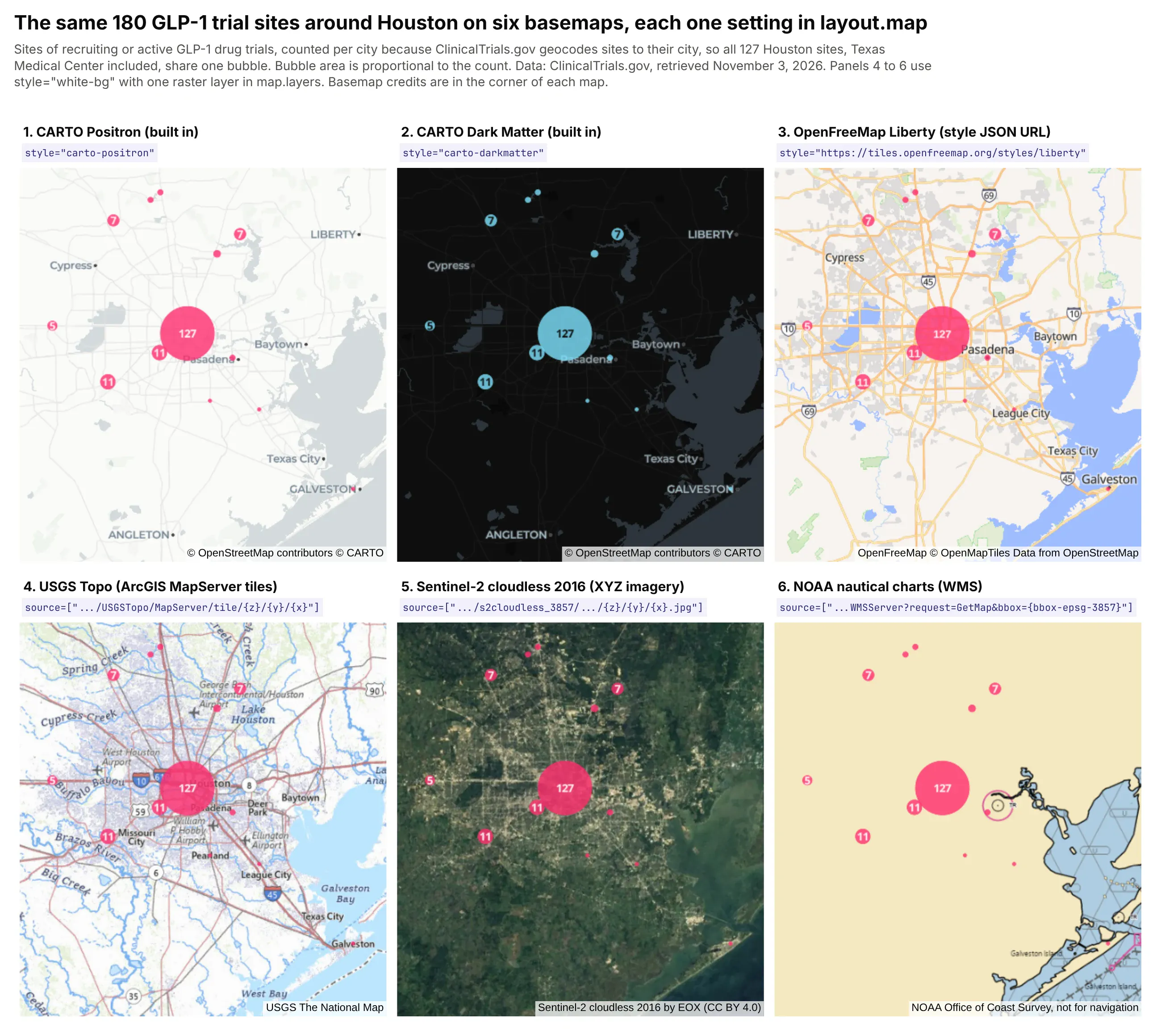
Technologies used: Plotly (make_subplots with map subplots, go.Scattermap, raster layers in map.layers).
Prompt: Draw the same set of points on six map subplots with the same center and zoom, each with a different basemap: carto-positron, carto-darkmatter, the OpenFreeMap liberty style URL (https://tiles.openfreemap.org/styles/liberty), USGS Topo tiles from basemap.nationalmap.gov's ArcGIS MapServer ({z}/{y}/{x}), Sentinel-2 cloudless 2016 tiles from EOX, and NOAA's nautical chart WMS with bbox={bbox-epsg-3857}. Label each panel with the one layout.map setting that produces it, and put each provider's credit in sourceattribution.
Basemap
Setting
Built-in styles
map_style="carto-positron", "carto-darkmatter", "carto-voyager", "open-street-map", "satellite" and others; none need a token
A MapLibre style JSON
map=dict(style="https://tiles.openfreemap.org/styles/liberty")
ArcGIS tiled MapServer
style="white-bg" and layers=[dict(sourcetype="raster", source=[".../MapServer/tile/{z}/{y}/{x}"], below="traces")]
XYZ imagery
The same, with the imagery server's URL template
OGC WMS, or an ArcGIS dynamic MapServer
The same, with bbox={bbox-epsg-3857} in a GetMap or /export URL
Your own vector tiles
A full MapLibre style dict in map.style with a vector source pointing at your tile server (see the vector tiles section below)
Two details catch people out. ArcGIS tile URLs put the row before the column ({z}/{y}/{x}), while most other servers use {z}/{x}/{y}. And every tile provider has its own terms: the built-in "satellite" style uses Esri World Imagery, CARTO's basemaps need a CARTO license for commercial use, and only the 2016 version of the Sentinel-2 cloudless mosaic is CC BY (later years are non-commercial). Put the provider's credit in sourceattribution so it shows in the corner of the map.
How to make large maps fast: millions of points and polygons
Energy, finance and pharma datasets outgrow a simple map quickly: hundreds of thousands of points, every census tract in a state, every branch of every bank. To find out which approach holds up at that size, we built one Dash app on real public data (566,902 points from public Oklahoma and Colorado well records, 84,000 census tracts and 52,244 lines from a public national dataset) and timed every library and technique we could on the same layers. Here's what we recommend:
What you're building
Approach
Why
A point map, up to about 100k points
Plotly Scattermap with NumPy arrays
Hover, click and lasso crossfilter with the rest of the app
A choropleth of counties or states
Plotly Choroplethmap, GeoJSON by URL, updates with Patch()
The geometry loads once, and recoloring sends a few KB
Census tracts, parcels or any layer of 10k+ polygons
Vector tiles from DuckDB or PostGIS in a Plotly map
The browser only loads what's on screen
500k+ points that all stay visible and clickable
deckgl-dash with binary arrays
GPU rendering with compact data
"How many are there here?" at any scale
H3 aggregation in SQL, or clustering
A few thousand rows instead of the whole table
Drawing, editing and measuring geometry
dash-leaflet EditControl and MeasureControl
Shapes come back to Python as GeoJSON
The chart below shows how long each library and technique took in that app to draw all 566,902 wells, from the first request until the map was ready:
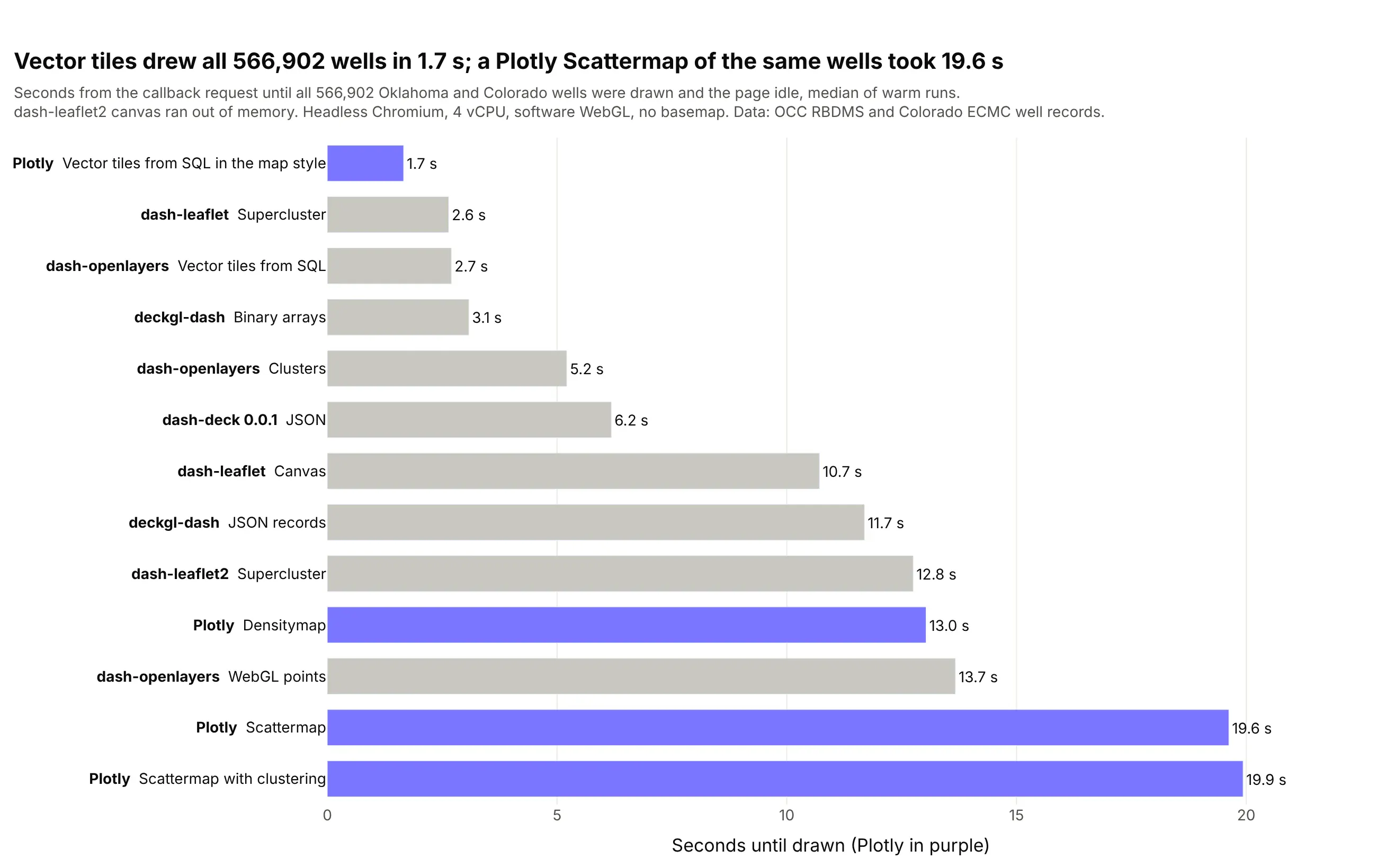
Three results matter most. A Plotly Scattermap is comfortable to about 100k points (3.7 s) and took 19.6 s for all 566k wells. Vector tiles drew the same wells in 1.7 s and 84,000 tracts in 1.9 s, because the browser only asks for the tiles in view. And keeping big GeoJSON out of the figure matters as much as the library: the same tract choropleth took 41.5 s with the GeoJSON inside the figure and 11.1 s with it loaded by URL. Our maps at scale deep dive has all three benchmark charts, the method, the Patch() timings, deck.gl and clustering code, and the patterns we use in large map apps.
Technologies used: Dash, Plotly (Scattermap, Densitymap, vector tiles in map.style), deckgl-dash, dash-leaflet, dash-openlayers, Playwright.
Prompt: Build one Dash benchmark app that draws the same 566,902 wells with each map library and technique (Plotly Scattermap with and without clustering, Densitymap, vector tiles, deckgl-dash with JSON and binary data, dash-leaflet, dash-openlayers), one per URL. Time each one in headless Chromium with Playwright from the callback request until the map is drawn and the page has been idle for 1.5 s, run each case three times, and plot the median of the warm runs as a horizontal bar chart.
Vector tiles from DuckDB or PostGIS: your own map service in Python
Vector tiles were the fastest way to draw big layers in every benchmark above, and they're how ArcGIS handles big layers too. An ArcGIS team would publish a layer like every watershed and stream in the country as a map service or a vector tile service on ArcGIS Server, and the browser would only ever download the part of it on screen. Python can do the same thing with vector tiles: the map is cut into a pyramid of square tiles, one set per zoom level, and each tile holds only the features inside it, simplified for that zoom, in the compact Mapbox Vector Tile (MVT) format.
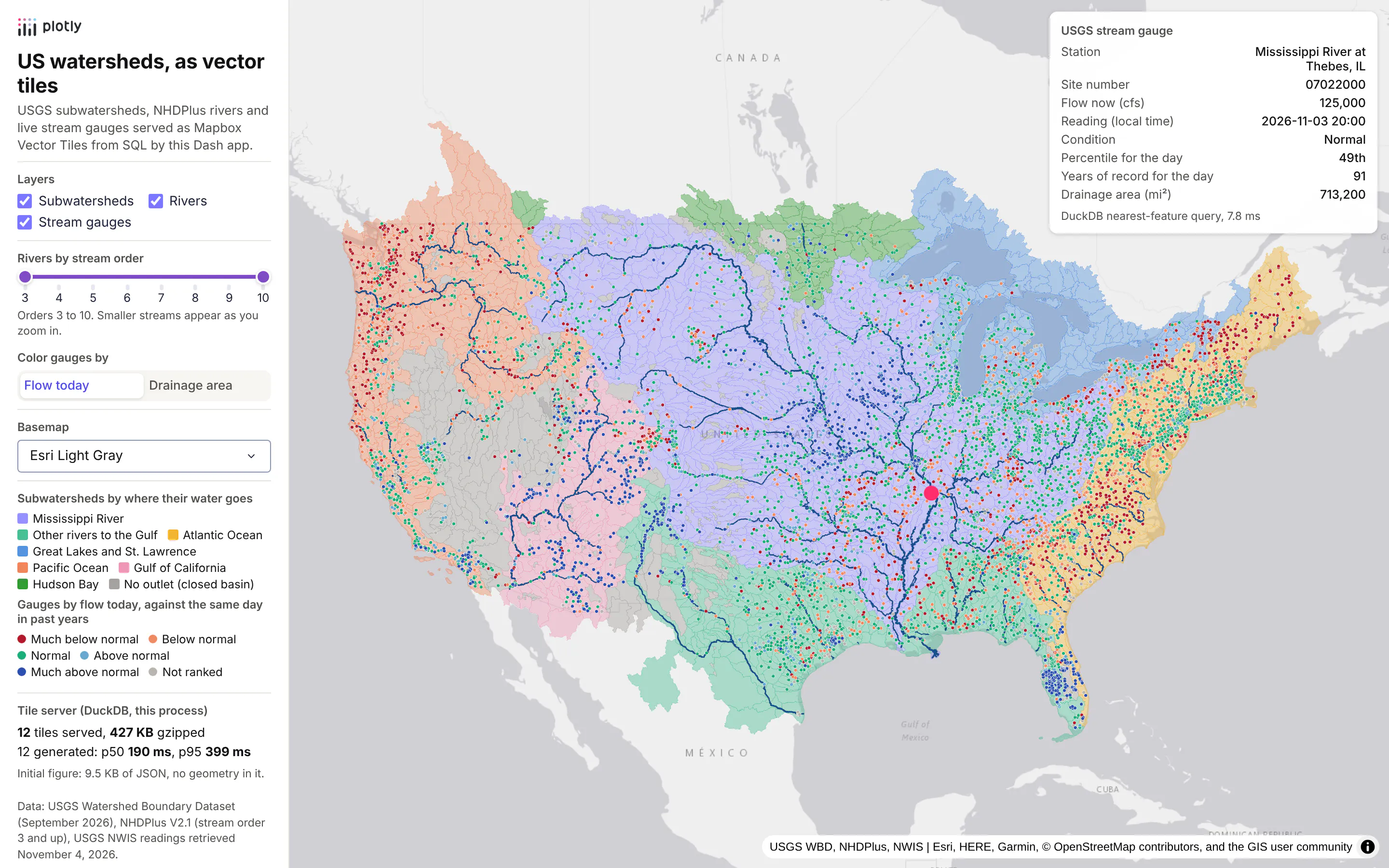
You don't need a tile server product or a tile package to make them. DuckDB's spatial extension and PostGIS both have an ST_AsMVT function that builds a tile from a SQL query, so one Flask route in a Dash app can serve tiles straight from a table as the browser asks for them. To show it on a real layer, we built a Dash app that serves three US hydrology layers that way: all 87,028 subwatersheds of the lower 48 (the smallest drainage areas in the USGS Watershed Boundary Dataset, known as HUC12s), shaded by where their water reaches the sea, 712,768 river reaches from NHDPlus, the national stream network from the EPA and USGS, leaving out the smallest headwater streams (stream order 1 and 2), and 8,082 USGS stream gauges colored by how today's flow compares with the same day in past years.
Technologies used: DuckDB spatial (ST_AsMVT, ST_AsMVTGeom, ST_TileEnvelope) or PostGIS, Flask, Dash, Plotly (a MapLibre style in layout.map.style), GeoPandas.
Prompt: Build a Dash app with a Flask route at /tiles/<layer>/<z>/<x>/<y>.pbf that serves Mapbox Vector Tiles from DuckDB's spatial extension using ST_TileEnvelope, ST_AsMVTGeom and ST_AsMVT, over three layers loaded from GeoParquet: USGS WBD HUC12 subwatersheds, NHDPlus rivers of stream order 3 and up, and active USGS stream gauges. Store the geometry in EPSG:3857 with an R-tree index and a simplified column for zooms below 8, and gzip and cache each tile. Draw the tiles in a Plotly map through a full MapLibre style in layout.map.style with vector sources and data-driven paint expressions, and add layer toggles and a stream order slider that Patch the style's layers.
The screenshot above shows that app over the whole lower 48. Sent as GeoJSON, its three layers are 1.3 GB (339 MB gzipped), most of it the 40 million vertices of the subwatershed outlines. As vector tiles, the first view of the lower 48 took 12 tiles and 427 KB gzipped, the figure itself was 9.5 KB of JSON with no geometry in it, and zooming into the confluence of the Mississippi and the Ohio fetched 12 more tiles and 140 KB.
The tile route
This is the core of it, with the same query in both dialects. The real version in the app adds a cache and per-zoom rules for each layer:
TILE_SQL = {"DuckDB": """SELECT ST_AsMVT(t, '{layer}', 4096, 'geom') FROM (SELECT {cols}, ST_AsMVTGeom({geom}, ST_Extent(ST_TileEnvelope($z, $x, $y)), 4096, 64, true) AS geomFROM {layer} WHERE ST_Intersects({geom}, ST_TileEnvelope($z, $x, $y))) t""","PostGIS": """SELECT ST_AsMVT(t, '{layer}', 4096, 'geom') FROM (SELECT {cols}, ST_AsMVTGeom({geom}, ST_TileEnvelope(%(z)s, %(x)s, %(y)s), 4096, 64, true) AS geomFROM {layer} WHERE {geom} && ST_TileEnvelope(%(z)s, %(x)s, %(y)s)) t""",}@server.route("/tiles/<layer>/<int:z>/<int:x>/<int:y>.pbf")def tiles(layer, z, x, y):sql = TILE_SQL[DIALECT].format(layer=layer, cols=COLS[layer], geom="geom_lo" if z < 8 else "geom")body = db.execute(sql, {"z": z, "x": x, "y": y}).fetchone()[0] or b""return flask.Response(gzip.compress(body), headers={"Content-Type": "application/vnd.mapbox-vector-tile","Content-Encoding": "gzip", "Cache-Control": "public, max-age=3600"})
The tables store each geometry more than once in Web Mercator (EPSG:3857, the projection tiles use): geom at full detail and geom_lo simplified to 500 m for zoomed-out tiles, and every geometry column has a spatial index (an R-tree in DuckDB, GiST in PostGIS), so each tile query reads only the features it needs. Zoomed out, the app also leaves the small streams out of the river tiles and reads the subwatersheds dissolved into 2,425 shapes, since at that scale the map only draws their fill color.
Drawing tiles in a Plotly map
On the Plotly side, a vector source in a full MapLibre style dict in layout.map.style points at the route, and MapLibre's paint and filter expressions do the styling. Restyling then costs almost nothing: in the app above, moving the stream order slider, recoloring the gauges by drainage area or switching the basemap sends a 2.0 to 2.7 KB Patch of the style and fetches no vector tiles at all. Tile features don't send Plotly's hoverData or clickData, so the app listens for clicks on the MapLibre map and finds the nearest feature in SQL, which took 7.8 ms for the Mississippi River gauge at Thebes, Illinois in the screenshot.
The recording below shows those interactions in the hydrology app, from the first view of the lower 48 to a zoom, a gauge click, the layer toggles and a basemap switch:
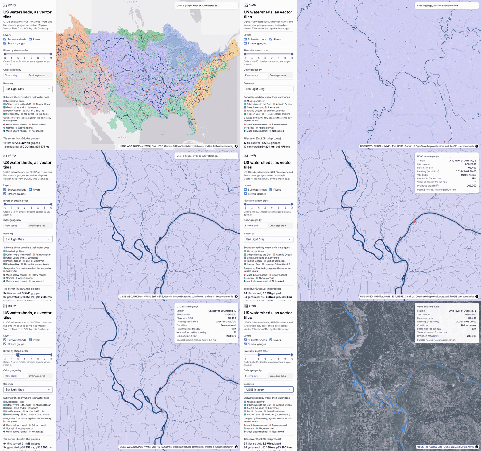
When we timed the same tile queries in both databases, both were fast enough that the browser, not SQL, set the pace: a warm median of 10.0 ms per tile in DuckDB 2.0 and 2.7 ms in PostGIS 3.4. DuckDB runs inside the Python process and reads GeoParquet directly, and PostGIS is the better fit when the data is shared, updated continuously or already lives there. Our vector tiles deep dive walks through two complete apps step by step, with prompts for a coding agent, the four changes that took its slowest zoomed-out census tract tile from 8.0 s to 1.1 s in DuckDB and 66 ms in PostGIS, server-side filtering, click handling and 3D columns.
How to make a Google Maps-style route map in Python
When people picture a map app, many of them picture Google Maps: pick a start and an end, and the app draws the fastest way there on a street map you can zoom into building by building. Teams ask for the same thing inside their own tools, such as drive times from a branch to its customers, the walk from a train station to a site, or which places a field crew can reach in half an hour. Python can do this for a city or a region with four open-source pieces: the street network from OpenStreetMap, a graph library that finds the fastest path through it, a street-level basemap, and a Dash app that turns clicks into routes.
To show how it fits together, we built a small route finder for Chicago on OpenStreetMap data. You click a start and an end, and a Dash callback finds the fastest walking or driving route and draws it with its distance and time. The recording below walks from Cloud Gate in Millennium Park to Navy Pier, switches to driving, routes from Buckingham Fountain to Navy Pier, and zooms in to street level on Lake Shore Drive:

There are limits to what this does. Our routes use each road's speed limit from OpenStreetMap (or a typical speed for its road type when there isn't one), so they don't know about traffic, turn costs or road closures, and they don't give spoken turn-by-turn directions. For that, or for routing across a whole country, the usual next step is a routing engine you run yourself, such as OSRM, Valhalla or GraphHopper, which all route on OpenStreetMap data and answer over HTTP, or a paid service such as the Google Maps Platform, Mapbox or Esri's routing service when live traffic matters.
Get the street network from OpenStreetMap with OSMnx
OSMnx downloads the streets of any place in OpenStreetMap and turns them into a graph, where every intersection is a node and every stretch of street between two intersections is an edge with its length, its name and its geometry. It also adds a speed and a travel time in seconds to every edge, which is what you want to minimize for a fastest route. The drivable streets in a box around Chicago came to 113,651 nodes and 286,278 one-way edges, and the walking network of downtown and the Near North and Near South sides to 28,811 nodes and 90,010 edges.
Technologies used: OSMnx, NetworkX. Data: OpenStreetMap contributors (ODbL), Chicago extract from BBBike.org.
Prompt: Use OSMnx to download the drivable street network of Chicago, add edge speeds and travel times in seconds, and save it as GraphML. Then find the fastest route between Wrigley Field and the Field Museum with NetworkX, weighted by travel_time, and print its length in kilometers and its time in minutes.
This will create code like this:
import networkx as nximport osmnx as oxG = ox.graph_from_place("Chicago, Illinois, USA", network_type="drive")G = ox.add_edge_speeds(G) # km/h from maxspeed tags, or the average for the road typeG = ox.add_edge_travel_times(G) # seconds per edgeorig = ox.nearest_nodes(G, X=-87.655536, Y=41.94827) # Wrigley Field (lon, lat)dest = ox.nearest_nodes(G, X=-87.617999, Y=41.8653) # Field Museumroute = nx.shortest_path(G, orig, dest, weight="travel_time")km = sum(G.edges[u, v, 0]["length"] for u, v in zip(route, route[1:])) / 1000
ox.graph_from_place downloads from OpenStreetMap's Overpass API. That service wasn't reachable from the machine we built this on, so our build script reads the same data from a downloaded OpenStreetMap extract of Chicago and filters the roads the way OSMnx's network_type="drive" and "walk" do. The fastest drive from Wrigley Field to the Field Museum on that graph is 11.7 km and about 12 minutes, by Clark Street and Lake Shore Drive.
Which Python library finds routes fastest?
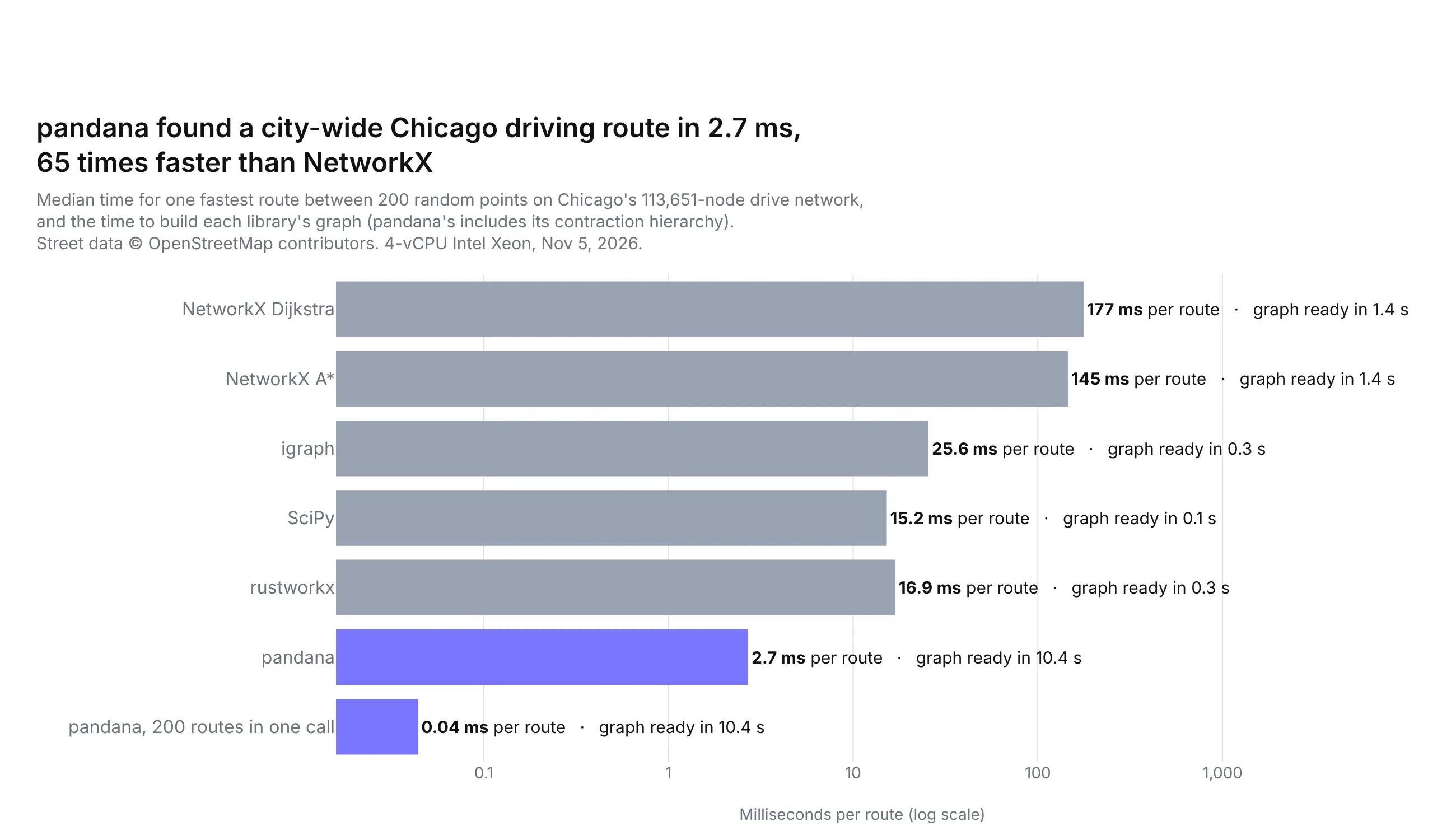
Once the streets are a graph, any graph library can find the fastest path, and there are five common ones in Python. We loaded the same Chicago driving graph into each of them and timed one fastest route between 200 random pairs of points across the city (a median drive of 22 minutes), checking every answer against NetworkX:
Technologies used: NetworkX, igraph, SciPy (scipy.sparse.csgraph), rustworkx, pandana, OSMnx. Data: OpenStreetMap contributors.
Prompt: Load a Chicago drive network from OSMnx into NetworkX, igraph, a SciPy sparse matrix, rustworkx and pandana, all from the same edge arrays weighted by travel_time. Time how long each takes to build, then time one fastest route between 200 random node pairs with each library, check that every route time matches NetworkX's Dijkstra, and plot the median milliseconds per route on a log-scale bar chart.
The libraries fall into three groups:
- NetworkX is the one OSMnx returns, written in pure Python, and the easiest to start with. At a median of 177 ms for a city-wide route (145 ms with A*, which steers the search toward the destination), it's fine for a few routes at a time but slow for thousands.
- igraph, SciPy and rustworkx run the same Dijkstra search in C, C++ or Rust and took 15 to 26 ms per route, about seven to twelve times faster than NetworkX, after a graph build of a third of a second or less. rustworkx has the closest API to NetworkX, so it's the easiest switch, and SciPy is already installed almost everywhere.
- pandana preprocesses the graph into contraction hierarchies, which add shortcut edges so that each search only has to look at a small part of the graph. That took 10.4 s up front, and then a route took 2.7 ms, or 0.04 ms when it computed 200 routes in one call. It computed 100,000 random route times in 2.3 s, which is what you want for an accessibility analysis such as drive time from every customer to the nearest branch.
Every library returned the same fastest route time as NetworkX's Dijkstra on all 200 routes, except pandana, which matched it to within 0.26 s.
Draw a route at street level
A route is a list of nodes, and each edge on it carries the street's real geometry, so joining those coordinates gives a line that follows every curve of the streets. Plotly draws it with go.Scattermap in line mode, and a street basemap comes from passing a MapLibre style URL to layout.map.style. We used OpenFreeMap's Liberty style, free vector tiles of OpenStreetMap data with street names, transit stops and 3D buildings, and no API key:
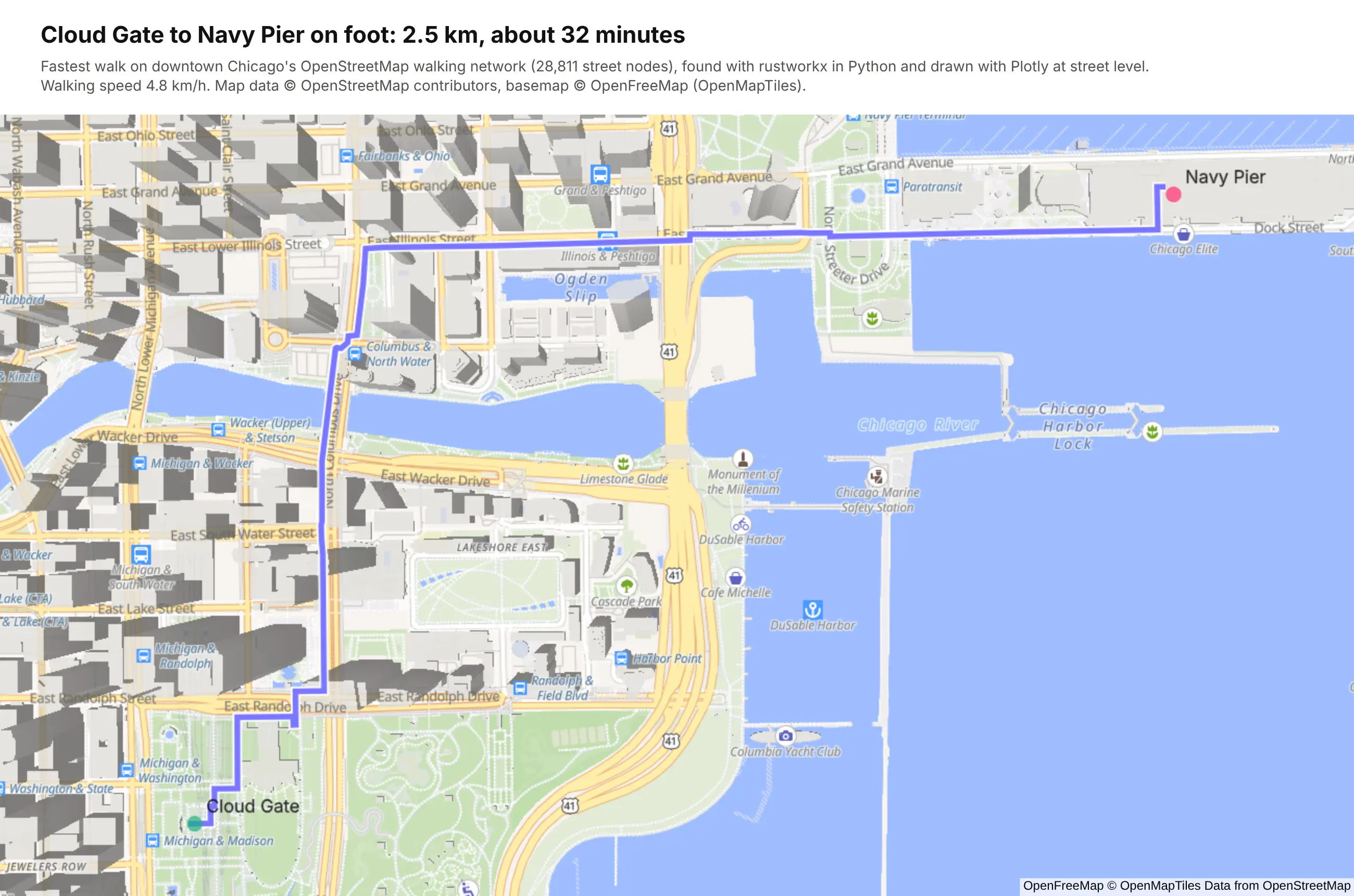
Technologies used: Plotly (go.Scattermap, a MapLibre style URL in layout.map.style), rustworkx, OSMnx. Data: OpenStreetMap contributors; basemap © OpenFreeMap (OpenMapTiles).
Prompt: Find the fastest walk from Cloud Gate to Navy Pier on an OSMnx walking network of downtown Chicago with rustworkx, join each edge's geometry into one line, and draw it with go.Scattermap as a purple line over a white outline, with green and pink markers at the start and end, on the OpenFreeMap Liberty style (https://tiles.openfreemap.org/styles/liberty) at zoom 15, titled with the distance and walking time at 4.8 km/h.
This will create code like this:
import plotly.graph_objects as golats, lons = [], []for u, v in zip(path, path[1:]): # path: the route's node idsxs, ys = G.edges[u, v, 0]["geometry"].xy if "geometry" in G.edges[u, v, 0] else ([G.nodes[u]["x"], G.nodes[v]["x"]], [G.nodes[u]["y"], G.nodes[v]["y"]])lons += list(xs)lats += list(ys)fig = go.Figure([go.Scattermap(lat=lats, lon=lons, mode="lines", line=dict(width=9, color="white")),go.Scattermap(lat=lats, lon=lons, mode="lines", line=dict(width=5.5, color="#7A76FF")),])fig.update_layout(map=dict(style="https://tiles.openfreemap.org/styles/liberty",center=dict(lat=41.887, lon=-87.614), zoom=15.1), showlegend=False)
The same map.style setting takes any MapLibre style, so you can swap in CARTO's Voyager style, Esri's World Street Map tiles or your organization's own basemap.
Click to route in a Dash app
The Dash app adds the "click a start and an end" part. One thing to know first is that a Plotly map only reports clicks on its own markers, not on empty parts of the basemap. The app gets around that by drawing every node of the downtown walking network as a nearly invisible dot, so a click anywhere on a street lands on one, and by labeling the landmarks so you can click those too. A dcc.Store keeps the clicked points, and a second callback routes between them with whichever library is picked in the dropdown:
Technologies used: Dash (dcc.Store, clickData), Plotly, rustworkx, SciPy, NetworkX, OSMnx. Data: OpenStreetMap contributors; basemap © OpenFreeMap.
Prompt: Build a Dash app with a full-height Plotly map of downtown Chicago on the OpenFreeMap Liberty style and a sidebar with Walking/Driving radio items and a dropdown of path-finding libraries (rustworkx, SciPy, NetworkX). Draw every node of the OSMnx walking network as a nearly transparent marker so clicks anywhere on a street register, keep the last two clicked points in a dcc.Store, snap them to the nearest node of the walk or drive graph, find the fastest route by travel time, draw it as a purple line, and show the minutes, kilometers, the time the library took and the main streets in the sidebar. Keep the map's zoom with uirevision.
This will create code like this:
@app.callback(Output("points", "data"), Input("map", "clickData"), State("points", "data"),prevent_initial_call=True)def add_point(click, points):p = click["points"][0]return [[p["lat"], p["lon"]]] if len(points) != 1 else points + [[p["lat"], p["lon"]]]@app.callback(Output("map", "figure"), Output("result", "children"),Input("points", "data"), Input("mode", "value"), Input("library", "value"))def draw(points, mode, library):if len(points) < 2:return figure(points, None), "Click where the route starts." if not points else "Click where it ends."(lat0, lon0), (lat1, lon1) = pointsres = ROUTERS[mode].route(lat0, lon0, lat1, lon1, library) # nearest nodes, then the fastest pathreturn figure(points, res), f"{res['seconds'] / 60:.0f} min, {res['meters'] / 1000:.1f} km"
A city-wide driving route took rustworkx a median of 16.9 ms in the benchmark above, so the route appears as soon as you click, and the libraries in the dropdown return the same route at different speeds.
Coming from Esri ArcGIS? How the concepts map to Python
Many teams that start mapping in Python come from ArcGIS. They have years of data in shapefiles and file geodatabases, layers published as feature services in ArcGIS Online or ArcGIS Enterprise, and dashboards built in ArcGIS Dashboards or Experience Builder. None of that has to be thrown away, because the Python geospatial stack reads the same formats and services. This table maps the ArcGIS concepts to their Python equivalents:
In ArcGIS
In Python
Notes
Shapefile, file geodatabase (.gdb), GeoPackage
gpd.read_file("parcels.shp"), gpd.read_file("data.gdb", layer="Wells")
GDAL's OpenFileGDB driver reads file geodatabases without an ArcGIS license; gpd.list_layers("data.gdb") lists the feature classes
Feature layer or feature service (REST)
A requests call to the layer's /query endpoint with f=geojson, then gpd.read_file
Page through with resultOffset, because services return a capped number of records per request (often 1,000 or 2,000)
Map image or tile service (basemap)
A raster layer in map.layers with the service's /tile/{z}/{y}/{x} URL
ArcGIS orders tile URLs z, y, x, so copy the order exactly; the basemaps section shows one
Image service (elevation, imagery)
A request to /exportImage, read into a NumPy array
Example 12 pulls USGS 3DEP elevation this way
Projections, WKIDs
gdf.to_crs(epsg=4326) with pyproj
EPSG codes match Esri WKIDs for common systems (4326, 3857, 4269, 26915)
Geoprocessing: Spatial Join, Buffer, Clip, Dissolve, Intersect
gpd.sjoin, .buffer, gpd.clip, .dissolve, gpd.overlay
Buffer in a projected CRS (meters), not in degrees
Field Calculator, Summary Statistics
pandas: df["rate"] = df.a / df.b, df.groupby(...)
The whole table is a DataFrame
Symbology: unique values, graduated colors, graduated symbols
color= with a categorical palette, color_continuous_scale=, size=
Class breaks: bin the column with pd.cut or mapclassify and color by the bins
Labels and pop-ups
text= and hovertemplate=
Hover templates take any column, with number formatting
Spatial Analyst rasters
NumPy, rasterio, xarray
A DEM is a 2D array
ArcGIS Dashboards, Experience Builder, Web AppBuilder
Filters, selections and linked charts are Python callbacks
ArcGIS Enterprise behind your firewall
Runs in your own cloud or data center, with SSO and per-app access
ArcPy scripts and ModelBuilder
Python scripts, scheduled jobs
Same language; GeoPandas, shapely and pyproj replace the arcpy module
Read an ArcGIS feature service into GeoPandas
Feature services are the most useful bridge, because many public agencies publish their GIS data that way, and so does your own ArcGIS organization. Every layer has a REST query endpoint that can return GeoJSON, which GeoPandas reads directly. This function pages through a whole layer:
Prompt: Write a Python function that reads every feature of an ArcGIS feature service layer into a GeoDataFrame: call the layer's /query endpoint with requests, f=geojson and outSR=4326, page through it with resultOffset and resultRecordCount, and let me pass where and outFields. Use it on the NIFC WFIGS interagency wildfire perimeters layer.
import geopandas as gpdimport requestsdef query_feature_service(layer_url, out_fields="*", where="1=1", page_size=2000):"""Every feature of an ArcGIS feature layer as GeoJSON, paging past maxRecordCount."""features, offset = [], 0while True:params = {"where": where, "outFields": out_fields, "outSR": 4326, "f": "geojson","orderByFields": "OBJECTID", "resultOffset": offset, "resultRecordCount": page_size}page = requests.get(f"{layer_url}/query", params=params, timeout=120).json()["features"]if not page:breakfeatures += pageoffset += len(page)return gpd.GeoDataFrame.from_features(features, crs=4326)fires = query_feature_service("https://services3.arcgis.com/T4QMspbfLg3qTGWY/arcgis/rest/services/WFIGS_Interagency_Perimeters/FeatureServer/0",out_fields="poly_IncidentName,poly_GISAcres,attr_POOState")
Asking for outSR=4326 makes the service return longitude and latitude, so the result goes straight onto a Plotly tile map. Ask only for the fields you need with outFields, and filter on the server with where (for example where="poly_GISAcres > 10000" for the larger fires), because downloading a whole national layer to keep a few features is slow.
Use your ArcGIS services as they are
Moving to Python doesn't mean leaving existing services behind, which matters while ArcGIS Server is still running. A feature service query with f=geojson is a GeoJSON API. A tiled MapServer is an XYZ tile URL, as in the basemaps section. A dynamic MapServer, which draws images on request, becomes a raster source when you point it at the /export endpoint with bbox={bbox-epsg-3857} in the URL, which MapLibre fills in for each tile:
Prompt: Add an ArcGIS dynamic MapServer to a Plotly map as a raster layer in layout.map.layers, pointing at its /export endpoint with bbox={bbox-epsg-3857}, bboxSR and imageSR 3857, a 256 by 256 transparent png32 image, drawn below the traces.
source = [".../MapServer/export?bbox={bbox-epsg-3857}&bboxSR=3857&imageSR=3857""&size=256,256&format=png32&transparent=true&f=image"]layers = [dict(sourcetype="raster", source=source, below="traces")]
This map of Houston mixes them in one Plotly figure: USGS Topo tiles from an ArcGIS tiled MapServer as the basemap, FEMA's 1% and 0.2% annual chance flood zones from the National Flood Hazard Layer's dynamic MapServer, live NOAA weather radar over OGC WMS (no rain was in view when it rendered), and 94 USGS stream monitoring sites from the USGS Water Data OGC API as a Plotly trace.
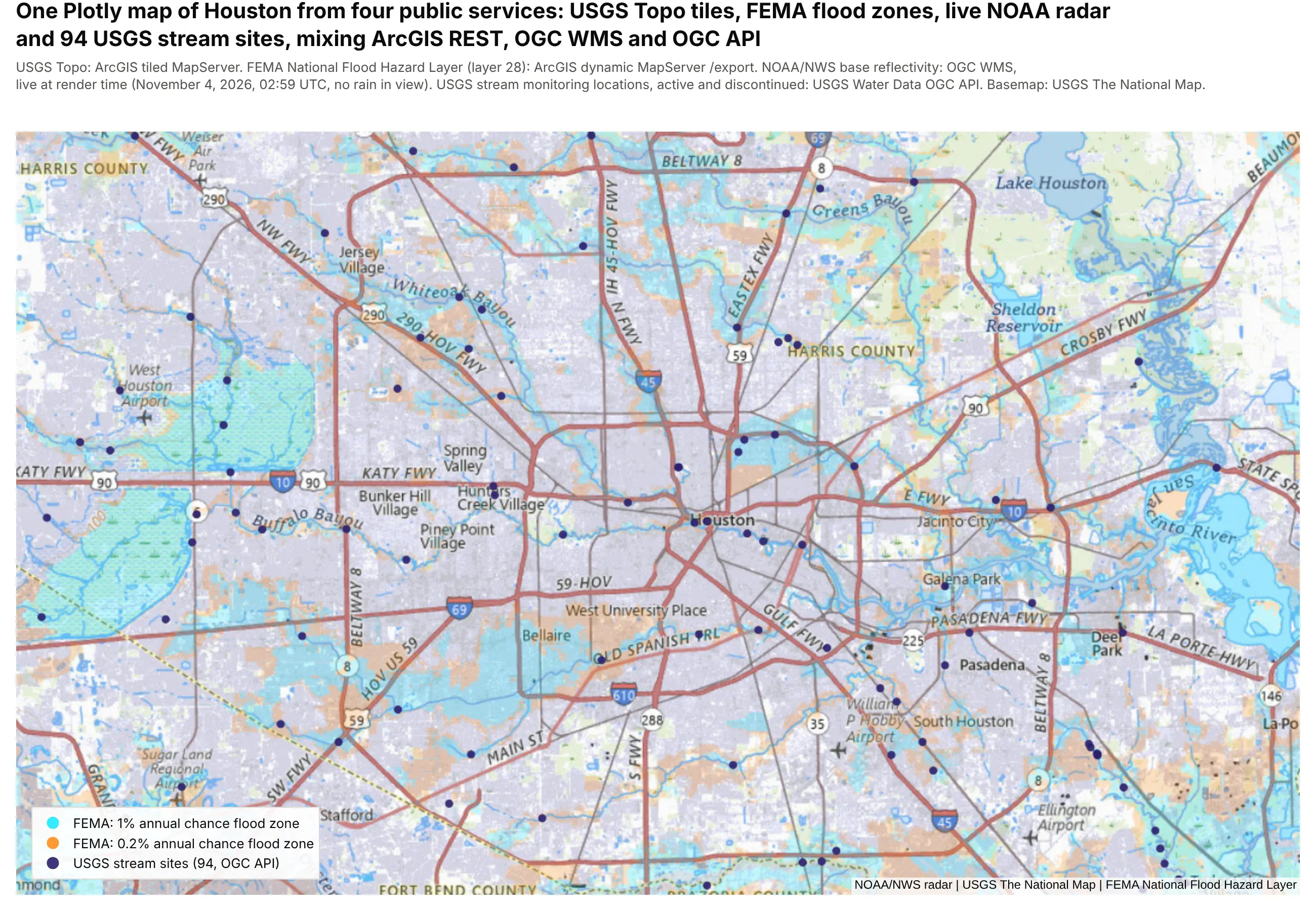
Technologies used: Plotly (go.Scattermap, raster sources in map.layers), requests.
Prompt: Make a Plotly map of Houston that mixes four public services: USGS Topo tiles from basemap.nationalmap.gov as the basemap, FEMA National Flood Hazard Layer flood zones from its dynamic MapServer /export endpoint, NOAA base reflectivity radar over OGC WMS GetMap, both as raster layers in map.layers with {bbox-epsg-3857}, and USGS stream monitoring sites from the USGS Water Data OGC API drawn as a go.Scattermap trace.
The same goes for analysis. Our maps at scale deep dive has an example of this: it pulls the current wildfire perimeters from NIFC's public ArcGIS feature service, buffers them by 5 miles in DuckDB and joins them against census tracts with their population, finding 918,279 people within 5 miles of the 70 wildfires NIFC was tracking on November 4, 2026, along with the spatial SQL lessons we learned along the way.
Things that catch out ArcGIS users
- Data in a projected or older coordinate system. Some federal datasets are still published in NAD27 (EPSG:4267), Census files come in NAD83 (EPSG:4269), and many state datasets come in State Plane or UTM. Plotly tile maps expect longitude and latitude in WGS84, so call to_crs(epsg=4326) first. Between NAD27 and WGS84 the shift is tens of meters, which won't make the map look wrong, so it's easy to miss.
- Lengths and areas in degrees. gdf.length on longitude and latitude returns degrees. Measure in an equal-area or local projected CRS, or use pyproj.Geod(ellps="WGS84").geometry_length(geom) for geodesic lengths, and measure before you simplify a geometry, because simplifying shortens lines.
- Shapefile field names are cut to 10 characters. STATUS_CODE arrives as STATUS_COD. File geodatabases and GeoPackages keep full names.
- Big geometries make big web pages. A county layer at full resolution can be tens of megabytes of GeoJSON. Simplify with gdf.simplify(0.001) (in degrees, about 100 m) and round coordinates before you draw it in a browser.
- A tile service covers different areas at different zoom levels. The USGS imagery basemap switches to aerial photos near the coast at higher zooms and returns empty tiles over open water, so check the tiles at the zoom you'll show.
Coming from Spotfire? How marking, filters and map layers translate to Dash
Spotfire users think in marking (select rows in one visualization and every other one follows), a filters panel, details-on-demand and a map chart with layers. Dash has a direct equivalent for each, written as Python callbacks instead of configured in a dialog:
In Spotfire
In Dash
Notes
Marking
selectedData (box or lasso on the map) and clickData, stored in a dcc.Store that other callbacks read
Every chart, grid and map can mark and be marked
Filters panel
dcc.Dropdown, dcc.Checklist, dcc.RangeSlider, or the column filters in Dash AG Grid
Filters run in pandas, DuckDB or your database
Details-on-demand
A clickData callback that looks up the row and fills a card or a grid
Map chart marker, feature and image layers
Plotly map traces, plus raster and vector layers in map.layers
Map chart WMS and TMS layers
Raster layers in map.layers with the service URL
Same services, same URLs
Zoom visibility on a layer
minzoom and maxzoom on each layer
Data functions (TERR, Python) and IronPython scripts
Python in the callbacks
The whole app is Python
Information links and data connections
SQL from Python: your warehouse, PostGIS or DuckDB
Bookmarks
App state in the URL with dcc.Location
Spotfire Server and Library
Dash Enterprise or Plotly Cloud
Access control per app, with your SSO
The screenshot below comes from the benchmark app in our maps at scale deep dive, which maps 566,902 public oil and gas well records from Oklahoma and Colorado. Its operations dashboard is the Spotfire marking pattern, here filtered to 8 operators and 35,286 wells: lasso wells on the map and the bar chart, the KPI tiles and the AG Grid all filter to them, click a bar to filter by operator, and click a row to fly the map to that well.
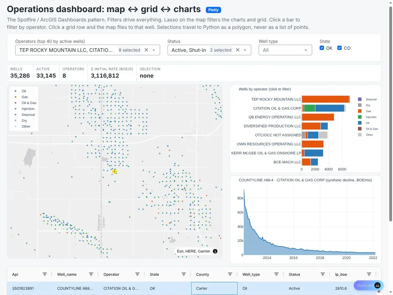
Technologies used: Dash (selectedData, clickData, dcc.Store), Plotly (go.Scattermap, bar and line charts), Dash AG Grid, DuckDB.
Prompt: Build a Dash operations dashboard for my wells table: a Scattermap of wells, a bar chart of wells by operator, a production decline curve, KPI tiles and a Dash AG Grid of wells. Store the current selection in a dcc.Store so a lasso on the map or the bar chart filters every other component, clicking a bar filters to that operator, and clicking a grid row flies the map to that well.
How to build an interactive map app with Dash
A map in a notebook answers one person's question. When a team needs to ask the same questions every week (which banks have branches in this metro, how much in deposits they hold there, what's at this address), it's worth building the map into an app once and sharing it, which is what ArcGIS Dashboards and Experience Builder do in the Esri world. Dash is the open-source Python framework for that, and the map in a Dash app is the same Plotly figure you already have.
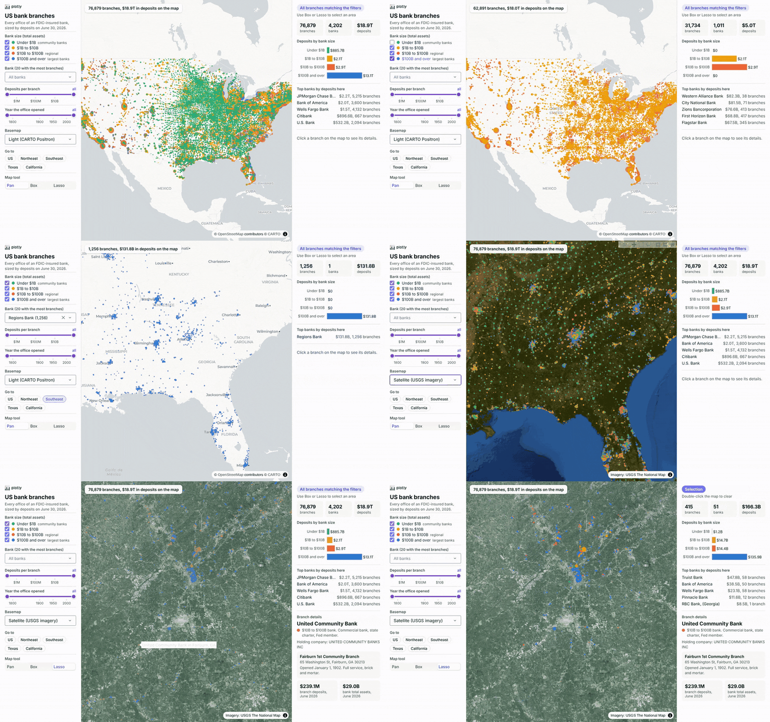
Here is a bank branch explorer built on the FDIC's BankFind data: all 76,879 offices of 4,202 FDIC-insured banks in the 50 states and DC, each sized by the deposits booked there in the Summary of Deposits for June 30, 2026 ($18.9 trillion in all) and colored by the size of the bank that owns it. The sidebar filters by bank size, by bank, by deposits per branch and by the year the office opened, switches between light, dark and USGS satellite basemaps and flies to a region. Drawing a box or lasso on the map fills the summary panel, and clicking a branch shows its details. Large banks book online and corporate deposits at a few offices, so some dots, and the totals of the areas that contain them, are much bigger than a typical branch.
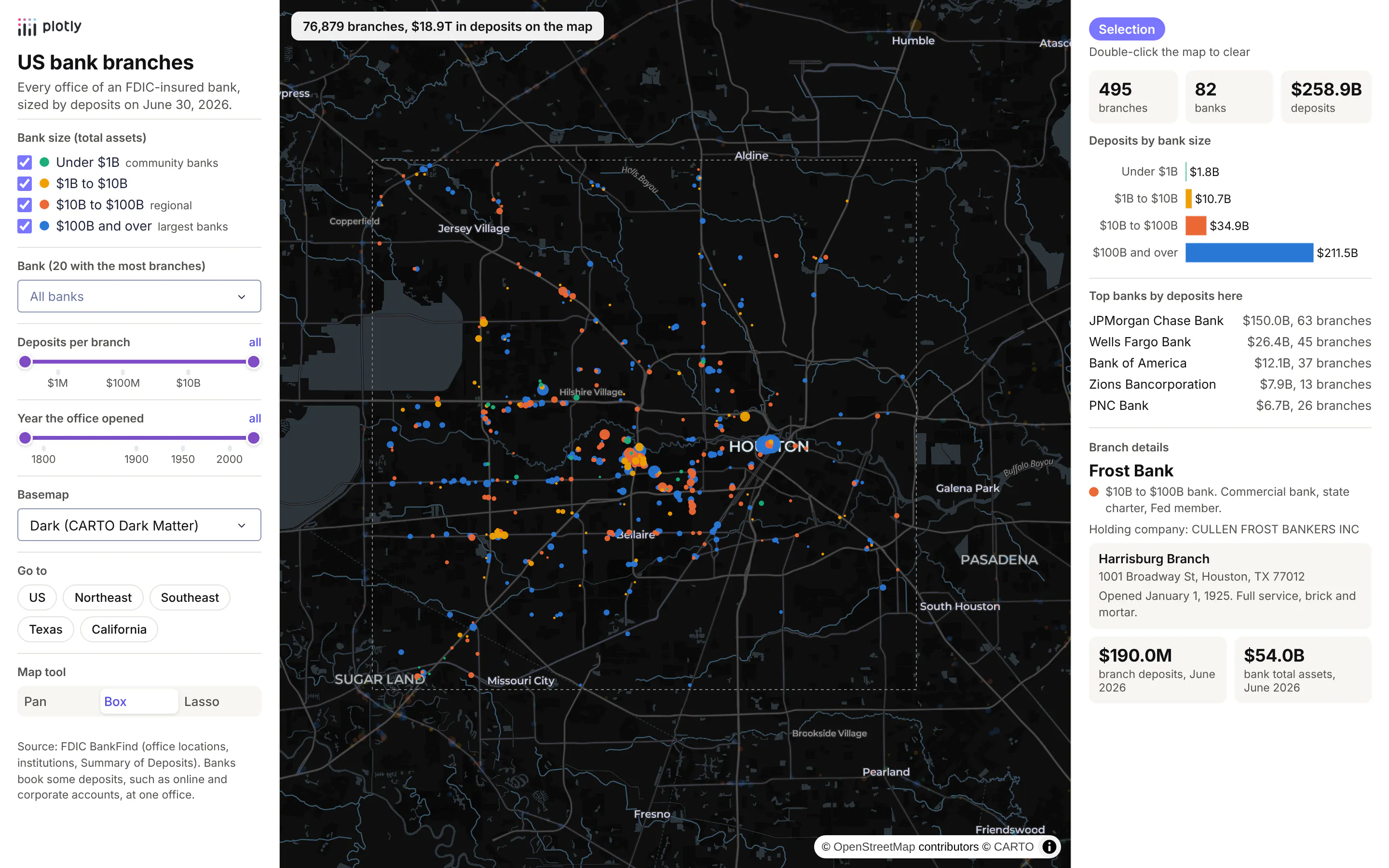
Technologies used: Dash (Patch, callbacks on selectedData and clickData), Plotly (go.Scattermap), pandas.
Prompt: Build a Dash app that maps every FDIC-insured bank office from the BankFind locations, institutions and Summary of Deposits APIs (api.fdic.gov) as one go.Scattermap with a trace per bank size class and marker size by branch deposits. Add a sidebar with size-class checkboxes, a bank picker, a deposits slider, a basemap dropdown and region buttons, each returning a dash.Patch instead of a new figure. Fill a summary panel with the branch count, deposits by size class and top banks for the box or lasso selection, and show a details card for the clicked branch.
In the recording below, the app hides the largest and the smallest banks, picks Regions Bank (1,256 branches), clears it, moves to satellite imagery over Atlanta, opens United Community Bank's Fairburn branch and selects the Atlanta metro with the lasso, which finds 415 branches of 51 banks holding $166.3B in deposits. The zoom and the lasso are sped up in the recording, because the headless browser we recorded in redraws 76,879 points slowly; everything else plays in real time:
How the app stays fast
The bank branch map holds all 76,879 offices as points, and sending the whole figure (4.6 MB of JSON) back to the browser every time someone ticks a checkbox would make it feel slow. Instead, the figure is sent once when the page loads, and every control after that returns a dash.Patch, which tells the browser to change only part of the figure. The map has one trace per bank size class, so the size checkboxes only send each trace's visible flag, which comes to 491 bytes:
Prompt: In my Dash app the map has one Scattermap trace per bank size class. Write a callback on the size-class checklist that returns a dash.Patch setting only each trace's visible flag, instead of rebuilding the figure.
from dash import Input, Output, Patch, callback@callback(Output("map", "figure"), Input("classes", "value"))def filter_points(classes):patch = Patch()for i, size_class in enumerate(TRACES): # one trace per bank size classpatch["data"][i]["visible"] = size_class in classesreturn patch
The bank picker and the sliders hide individual points, so they send the latitude arrays again with NaN for the points that are filtered out, encoded as base64 float32 (about 540 KB, a ninth of the full figure). Switching the basemap is the same idea as the checkboxes, with only the map style and the raster layer in the patch (284 bytes). Selections come back to Python as selectedData, with each point's row number stored in customdata, so the summary callback looks up the rows in pandas:
Prompt: Write a Dash callback on the map's selectedData that reads each selected point's row number from customdata, looks the rows up in my branches DataFrame, and returns the number of branches, the number of distinct banks (cert) and total deposits in billions.
@callback(Output("summary", "children"), Input("map", "selectedData"))def summarize(selected):rows = [p["customdata"] for p in selected["points"]] if selected else slice(None)sub = branches.iloc[rows]return f"{len(sub):,} branches, {sub.cert.nunique():,} banks, ${sub.deposits.sum() / 1e9:,.1f}B"
When we timed the bank branch app on the Dash development server, the filter callback took a median of 4 ms for a size checkbox and 6 ms for a bank change, and the summary callback 20 ms, across the 76,879 points. Setting uirevision on the figure keeps the user's zoom and pan while the filters change.
Share it
To put the app in front of a team, publish it to Plotly Cloud from the command line, which a coding agent can run for you:
Prompt: Publish this Dash app to Plotly Cloud: install dash[cloud], log me in with plotly user login and run plotly app publish.
pip install "dash[cloud]"plotly user loginplotly app publish
If the data has to stay inside your network, as it usually does for well data, trading positions or patient records, deploy to Dash Enterprise instead, which runs in your own cloud account or data center with your single sign-on, the way ArcGIS Enterprise does.
Interactivity in Dash: what you can and can't do with a map
Plotly maps in Dash send events to Python and accept partial updates from it, and most map apps are built from a handful of these:
You want
Use
Works with
A tooltip
hovertemplate with any columns from customdata
Map traces (Scattermap, Choroplethmap, Densitymap)
Click a feature to see its details
clickData in a callback
Map traces
Select with a box or lasso
dragmode="select" or "lasso", then selectedData
Scattermap and Choroplethmap
Query by what's on screen
relayoutData, which carries the map's center, zoom and visible corners (map._derived)
Any map
Keep the user's zoom when data changes
uirevision on the figure
Any map
Change part of the map without resending it
dash.Patch()
Anything in the figure
Respond without a server round trip
clientside_callback in JavaScript
Anything
Turn layers on and off
Legend clicks for traces, or a checklist that patches visible
Traces and map.layers
Show a layer only at some zooms
minzoom and maxzoom
map.layers
Tilt the map, or extrude polygons in 3D
map.pitch and a fill-extrusion layer in the style
Any map
And some things Plotly maps don't do today, with what to use instead:
- No hover or click on map.layers. Raster, GeoJSON and vector tile layers in layout.map.layers are drawn by MapLibre but don't send hoverData or clickData. Put features people need to click in a trace, or take the click position from a transparent trace and look up the nearest feature in SQL.
- No paint or filter expressions on map.layers entries. A layer takes one color, width and opacity. For styling by value (color by diameter, filter by year), give map.style a full MapLibre style dict with your own layers, which takes any MapLibre expression and can be patched from a callback.
- No drawing, editing or measuring tools on maps. Plotly's shape-drawing tools work on regular charts only. For sketching a polygon, editing a boundary or measuring a distance, use dash-leaflet, whose EditControl returns shapes to Python as GeoJSON.
- Web Mercator only on tile maps. For an Albers, Robinson or orthographic map, use the outline traces (Scattergeo, Choropleth), which have projections but no tiles.
- Not millions of individual points. In our benchmark of Oklahoma and Colorado oil and gas well records, a Scattermap was comfortable to about 100k points (3.7 s) and took 19.6 s for all 566k wells. Past that, use vector tiles, H3 aggregation or deck.gl, as the large maps section above shows. Plotly's built-in clustering gets slow at that size, so cluster with dash-leaflet or aggregate instead.
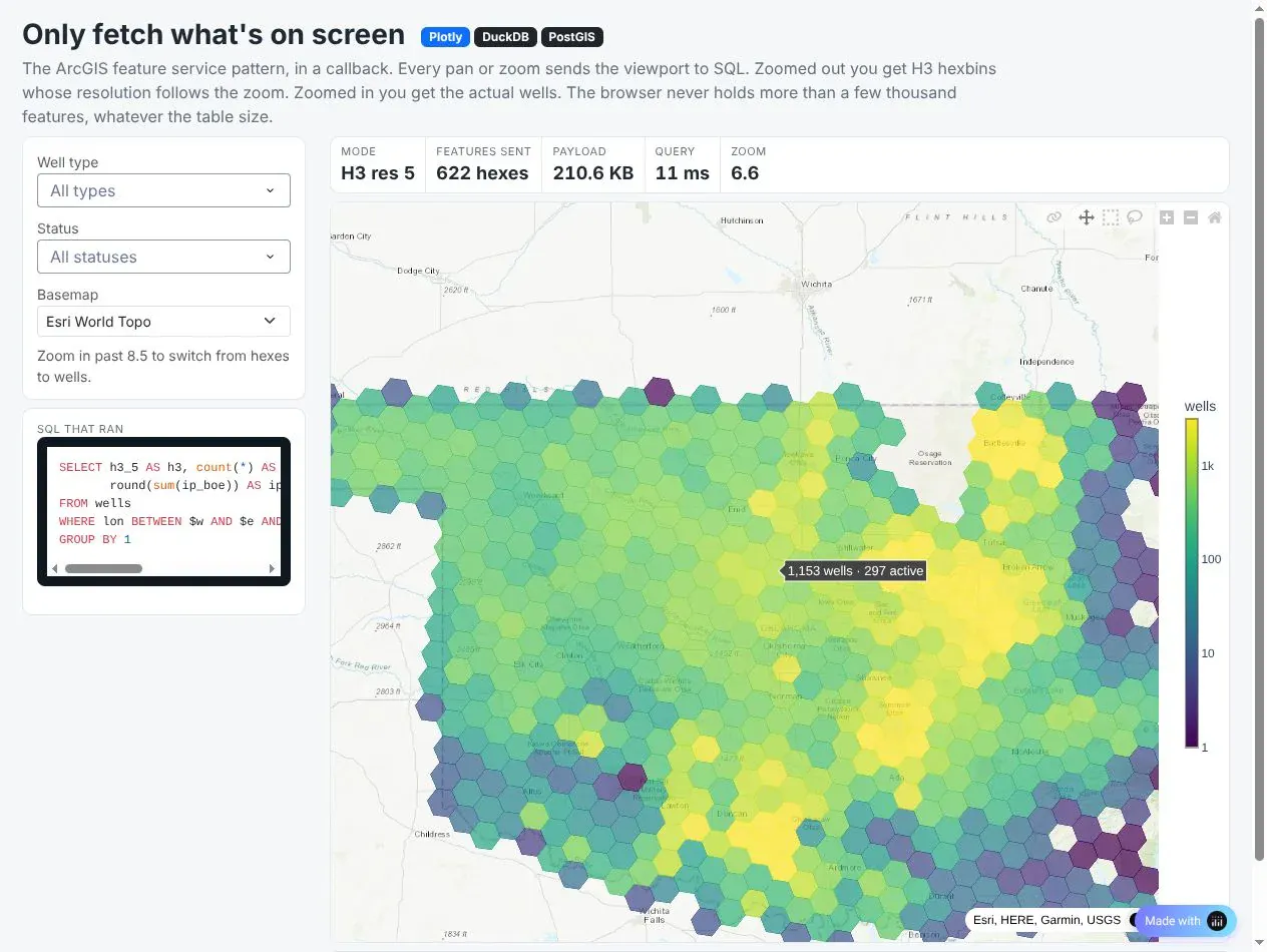
Two patterns do most of the work in large map apps. Viewport queries send the visible area to SQL on every pan and zoom. In the well map from our benchmark app, the query returns H3 hexagons of well counts when zoomed out and individual wells when zoomed in, so the browser never holds more than a screenful. That's how an ArcGIS feature service behaves:
Prompt: Write a Dash callback on the map's relayoutData that reads the visible corners from map._derived, and when zoomed out below 8.5 runs a DuckDB query counting wells per H3 resolution 5 cell inside that box and draws them as a hexagon choropleth, otherwise draws the individual wells in view, returning a dash.Patch of the first trace.
@callback(Output("map", "figure"), Input("map", "relayoutData"))def load_view(relayout):corners = relayout["map._derived"]["coordinates"] # four [lon, lat] cornersw, s, e, n = bbox(corners)p = Patch()if relayout.get("map.zoom", 6) < 8.5:hexes = duck.execute("SELECT h3_5, count(*) AS wells FROM wells WHERE lon BETWEEN ? AND ? ""AND lat BETWEEN ? AND ? GROUP BY 1", [w, e, s, n]).df()p["data"][0] = hex_choropleth(hexes)else:p["data"][0] = well_points(w, s, e, n)return p
This is that well map zoomed out over Oklahoma, where its panel shows the H3 resolution, how many hexagons came back, the payload size and the query time:
Technologies used: Dash (relayoutData, Patch), Plotly (go.Choroplethmap, go.Scattermap), DuckDB, h3.
Prompt: Add a panel to the viewport map that shows the H3 resolution, the number of hexagons returned, the payload size, the query time and the SQL that ran for the current view.
For sketching and measuring, dash-leaflet's EditControl returns drawn shapes to Python as GeoJSON, ready for a spatial query; the maps at scale deep dive shows the code, along with sending lasso selections to Python as a polygon instead of a list of points.
Deploying map apps on Dash Enterprise or Plotly Cloud
A map app deploys like any other Dash app. Dash Enterprise runs it inside your own cloud account or data center, next to your PostGIS database and behind your company's login, which is usually what an ArcGIS Server or Spotfire Server replacement needs. Plotly Cloud is the quickest way to share one. Three settings matter most for map apps: run one gunicorn process with many threads, because a map asks for 10 to 30 tiles at once; build tile URLs from the request's Origin header, because both platforms run apps behind an HTTPS proxy; and keep DuckDB's database file on the persistent filesystem (DASH_DATA_DIR), so tables and spatial indexes are built once. The vector tiles deep dive covers the rest.
How to make a map in Python with AI
Coding agents such as Claude Code, Codex, GitHub Copilot and Cursor write good Plotly map code, and most of the examples in this post started from a prompt. The results are best when the prompt names the data source, the coordinate system, the map type and the checks you want, because those are where map code goes wrong. A prompt like this one produces something close to example 4:
Make a Plotly map of the rivers of the United States.- Data: Natural Earth's 1:10m rivers and lake centerlines shapefile (plus the North Americasupplement). Read the zip with geopandas and reproject to EPSG:4326.- Keep the features inside the lower 48. Compute each river's geodesic length in km withpyproj.Geod before simplifying anything; print the total.- Draw the lines with go.Scattermap on carto-darkmatter, one trace per size class,lines joined with None, wider lines for bigger rivers.- Hover shows the river name and its length. Legend shows km per class.- Title states a real total; subtitle gives the source and basemap credit.- Save map.html (under 5 MB, simplify geometry if needed) and a PNG at 2x.
One thing we learned while building this guide: AI tools are careful with maps of critical infrastructure. Our first drafts used public government data on pipelines, LNG terminals, offshore platforms and power lines, and while we were staging the posts, an automated safety check stopped our coding agent partway through publishing the sections that combined those assets with hazards like hurricanes and wildfires. Nothing in them was secret, but the combination of where infrastructure is and what could hit it reads as sensitive, so we swapped in the weather, river, finance and clinical trial examples you see here. If your team maps its own pipelines, substations or plants, expect AI tools to slow down or refuse on that kind of map, and plan for those apps to be built and reviewed by people who are cleared to work with the data.
Plotly Studio is a desktop app where you point an AI at a dataset and it builds charts and a Dash app around your questions. Give it a table with coordinates and ask for the map and the controls you want:
Map every bank branch in this file as a bubble sized by deposits and colored by bank size, on a light basemap. Add a bank filter, a deposit slider and a panel that totals the deposits of whatever I select with the lasso.
Summary
Python can make every map a GIS analyst makes in ArcGIS or Spotfire, from the same shapefiles, geodatabases and feature services. GeoPandas reads and processes the data, Plotly draws it on any basemap you already use, DuckDB or PostGIS serve the layers too big for a browser as vector tiles, and Dash turns the result into an app with the selection and filtering your team is used to. Start with the map type that fits your data from the list of map types above, copy the closest example, and put your coordinates in longitude and latitude before you draw them.