
Chris Parmer
2026-11-03
How to Serve Vector Tiles from Python with DuckDB, PostGIS and Dash
TL;DR
- You can serve vector tiles from Python with one Flask route and one SQL query per tile. ST_TileEnvelope, ST_AsMVTGeom and ST_AsMVT build each tile on request, and both DuckDB's spatial extension and PostGIS have them. We built two example Dash apps this way for this post: a wells app, with every US census tract and the oil and gas wells in public Oklahoma and Colorado records, and a hydrology app, with US watersheds, rivers and stream gauges.
- A Plotly map in Dash draws the tiles through a MapLibre style, so the browser only downloads what's on screen. In the hydrology app, the three layers (87,028 USGS subwatersheds, 712,768 NHDPlus river reaches and 8,082 live stream gauges) are 1.3 GB as GeoJSON, and the first view of the lower 48 as tiles was 12 tiles and 427 KB gzipped.
- Four changes make tiles fast: a spatial index the query actually uses, simplified geometry for low zooms, skipping polygons smaller than a pixel, and one point per pixel when zoomed out. On the wells app's 84,000 census tracts they took the slowest zoomed-out tile from 8.0 s to 1.1 s in DuckDB 1.5.6 and 66 ms in PostGIS 3.4.
- The main DuckDB trap is a WHERE geom IS NOT NULL filter around the clipped rows, which makes DuckDB skip its spatial index (an R-tree). In the hydrology app on DuckDB 2.0 it took a river tile from 2.6 ms to 733 ms and a subwatershed tile from 7.8 ms to 49 s. Leave the filter out, or put the clipping step in a MATERIALIZED CTE (a named subquery DuckDB runs on its own first), which fixed it on both 1.5.6 and 2.0. We also hit a second slowdown that only happens in DuckDB 2.0, which compressed the big polygon column with ZSTD by default, and turning that compression off took a zoomed-in subwatershed tile from 88.8 ms to 7.6 ms.
- PostGIS built tiles faster at every zoom by the median (2.7 ms against 10.0 ms on the hydrology app's three layers), and DuckDB needs no server, since it runs inside the Dash app and reads GeoParquet directly.
This post shows how to build vector tile maps like these two, which draw layers of hundreds of thousands of features at full detail as you zoom in:
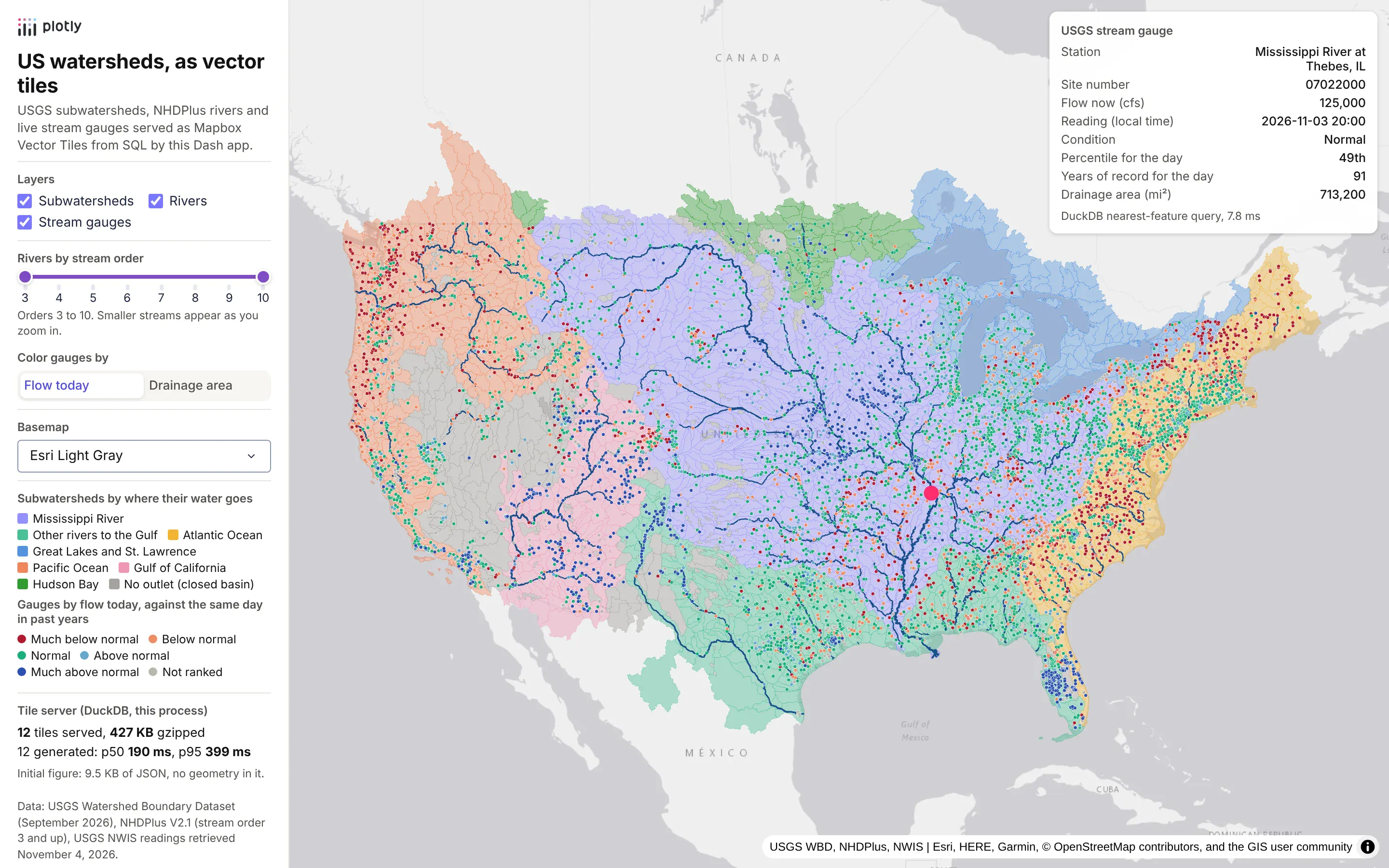
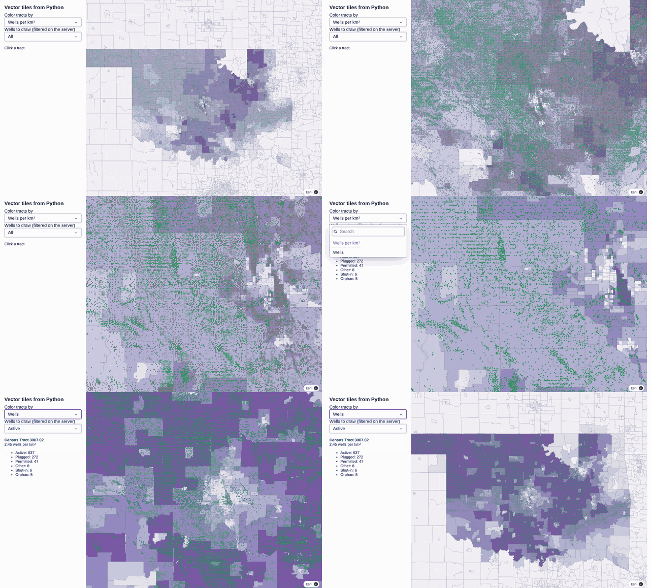
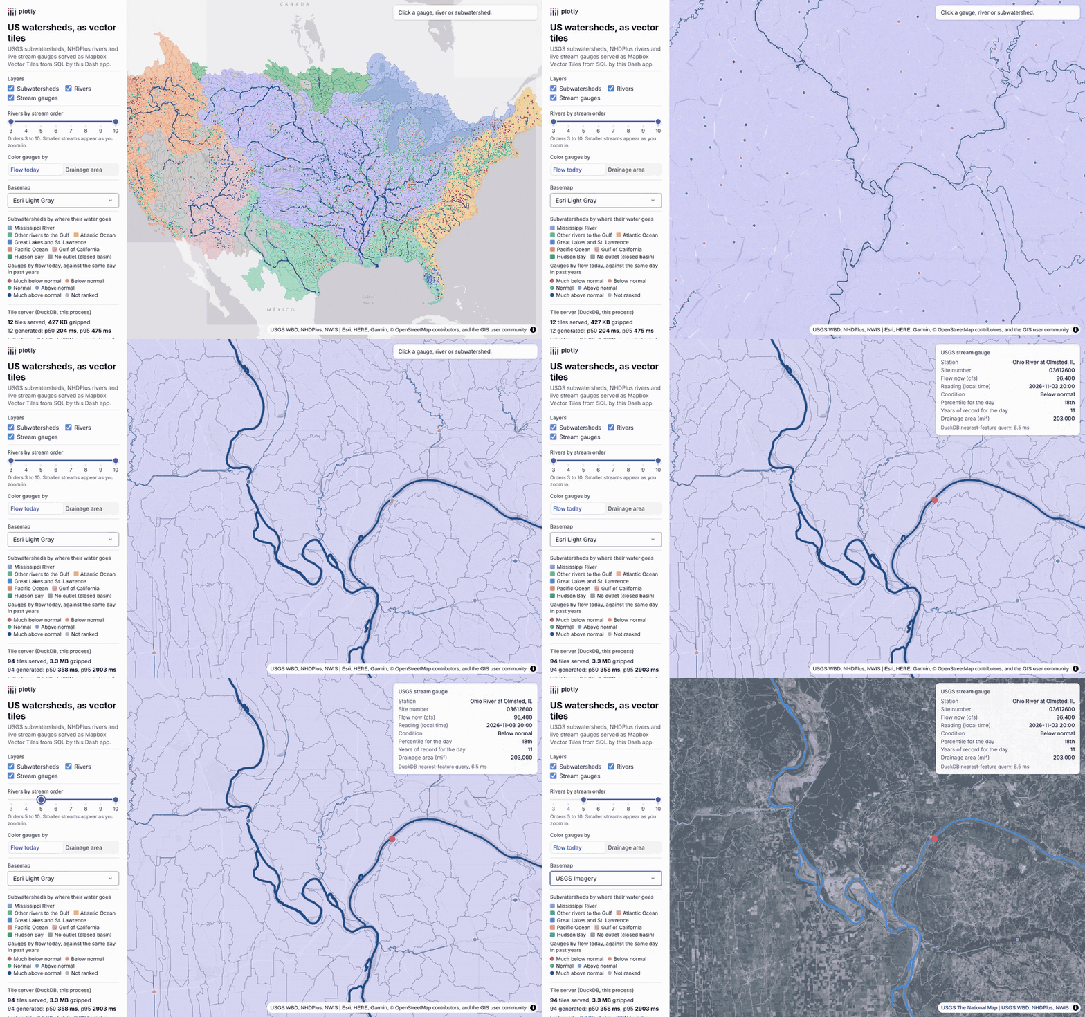
The map above is the hydrology app, with every subwatershed, river and stream gauge in the lower 48 and a gauge on the Mississippi selected. The prompt that builds it is in the hydrology section near the end of the post. The recording below is the wells app, with every US census tract and the oil and gas wells in public Oklahoma and Colorado records, zoomed in, clicked and filtered on the server. We build it in seven steps in the middle of the post, with a prompt for each step:
A lot of the teams we talk to in oil and gas and utilities are moving their maps off ArcGIS Server and Spotfire, usually because their analysis already lives in Python and they want the maps next to it. The data they want on those maps is big: every well in a basin, every watershed and stream in a region, every census tract in a service territory. On ArcGIS, a map service or a vector tile service takes care of that by sending the browser small pieces of the map as you pan and zoom, so nobody ever downloads the whole layer. When the same team rebuilds the map in Python, the first attempt usually sends every feature to the browser as GeoJSON, and it works until a layer reaches tens of thousands of shapes.
This post shows how to do the same thing in Python. A single Flask route turns a DuckDB or PostGIS table into vector tiles, and a Plotly map in a Dash app draws them. It walks through the two apps shown above. The wells app draws 84,119 census tracts and 566,902 oil and gas wells from Oklahoma and Colorado, and we build it step by step, with the prompt we gave a coding agent at each step. The hydrology app draws every subwatershed, river reach and live stream gauge in the lower 48, served from DuckDB and from PostGIS with the same queries, and we measured it on DuckDB 2.0. This post is the vector tiles deep dive in our Python maps guide, which covers every kind of map you can make in Python. Where this post compares tiles with other ways of drawing large maps in Dash (Plotly traces, deck.gl, dash-leaflet and dash-openlayers), the full benchmarks behind those comparisons are in our post on maps at scale in Dash.
What are vector tiles, and why serve them from Python?
Most web maps start out with GeoJSON. The app sends every feature to the browser up front at full detail, whether it's on screen or not. That's fine for a few thousand shapes, but it falls apart as layers grow. In our maps at scale benchmark, drawing about 84,000 US census tracts (the same layer as the wells app) as a Plotly choropleth took 11.1 s when the browser loaded the GeoJSON by URL and 41.5 s when the GeoJSON was inside the figure.
Tiles fix this by splitting the world into a pyramid of squares. At zoom 0 the whole world is one tile, and each zoom level splits every tile into four. The map works out which tiles cover the screen and requests only those. Each vector tile holds just the features inside its square, simplified for that zoom, with coordinates stored as integers on a grid (usually 4096 by 4096). The format is the Mapbox Vector Tile (MVT) specification, a compact protobuf that MapLibre, Mapbox, OpenLayers, deck.gl and Esri's own clients all read.
Serving the tiles from Python means the tile route sits on the same Flask server as your Dash callbacks, reads the same database, and can filter tiles by whatever the user picked in the app, with no separate tile server product to install or keep in sync.
Should you generate tiles from SQL or pre-generate them?
There are two ways to get vector tiles. You can generate every tile ahead of time with a tool like tippecanoe and save them into a single .pmtiles or .mbtiles file, or you can build each tile from SQL when the browser asks for it, which is what this post does. Tiles from SQL always show the current data, can be filtered per request, and need no build step, and with a cache in front they're fast enough for most apps.
If your data changes once a quarter and nobody needs to filter it, a PMTiles file on object storage behind a CDN is hard to beat, because there's no database to run at all. Either way the tiles are the same MVT format, so you can switch later without touching the map.
What data do you need to make your own vector tiles?
A vector tile isn't built from any special map file. It's built from an ordinary table, one row per feature, with a geometry column (a point, a line or a polygon) and whatever other columns you want to color by or show on click. The tile route asks the table for the rows inside one square of the map and packs them into a tile, so if you can get your data into a DuckDB or PostGIS table with a geometry column, you can serve it as vector tiles. Nothing gets converted or uploaded ahead of time.
Here's where the data in this post's two examples started out:
- Oil and gas wells: a table of rows with a latitude and a longitude column, from the public well databases of the Oklahoma Corporation Commission and Colorado ECMC. The app makes a point from each row's two columns with ST_Point(lon, lat).
- Stream gauges: a tab-separated text file from the USGS water data service, one row per gauge with its latitude, longitude and latest flow. These are also made into points from two columns.
- Census tracts: polygons from the Census Bureau's TIGER/Line boundary files, which come as shapefiles, saved once as a GeoParquet file.
- Subwatersheds: polygons from the USGS Watershed Boundary Dataset, which comes as an Esri file geodatabase (a .gdb folder).
- Rivers: lines from an ArcGIS REST map service run by the US EPA, downloaded 2,000 features at a time.
So yes, if all you have is a spreadsheet or a CSV of latitude and longitude points, you can turn it into your own vector tile map. Load it, make a point from each row, transform the points to Web Mercator (EPSG:3857, the projection tiles use; plain latitude and longitude is EPSG:4326), and add a spatial index (an R-tree in DuckDB) so each tile query only reads the rows near its square:
Prompt: I have sites.csv with name, value, lat and lon columns. Load it into DuckDB with the spatial extension, make a point geometry from lon and lat, transform it to EPSG:3857 with always_xy, and add an R-tree index, so a Flask route can serve it as vector tiles.
This will create code like this:
import duckdbcon = duckdb.connect()con.load_extension("spatial")con.execute("""CREATE TABLE sites ASSELECT name, value,ST_Transform(ST_Point(lon, lat), 'EPSG:4326', 'EPSG:3857', always_xy := true) AS geomFROM read_csv('sites.csv')""")con.execute("CREATE INDEX sites_geom ON sites USING RTREE (geom)")
From there, the tile route in step 1 below works unchanged with sites in place of tracts. Note the order inside ST_Point: longitude first, then latitude, which is the opposite of how most people say coordinates out loud and the most common reason points end up in the wrong place.
The other common starting points need one different line each:
- A shapefile, file geodatabase, GeoPackage or GeoJSON file: DuckDB reads all of them with ST_Read('rivers.shp') (or ST_Read('data.gdb', layer := 'WBDHU12')), with the geometry already in a column. Check the file's coordinate system first. Our county shapefile came in NAD83 (EPSG:4269), so its transform starts from 'EPSG:4269' instead of 'EPSG:4326'.
- A GeoPandas GeoDataFrame: save it with gdf.to_parquet('layer.parquet') and read it in DuckDB with read_parquet. This is what we did for the tracts and the hydrology layers, because GeoParquet loads in seconds and keeps the coordinate system with the data.
- A table that's already in PostGIS: it already has a geometry column. Add a Web Mercator copy once with ST_Transform(geom, 3857) and a GiST index on it. A PostGIS table of plain latitude and longitude columns gets its points from ST_SetSRID(ST_MakePoint(lon, lat), 4326).
- An ArcGIS feature service: query its REST endpoint for GeoJSON page by page (f=geojson), or read it with gpd.read_file on the query URL, then save it as GeoParquet as above.
If your CSV has fewer than about 100,000 points, you may not need tiles at all. In our benchmark, a plain go.Scattermap drew 100,000 of the wells in 3.7 s with hover, click and lasso working, and that's a few lines of Plotly with no tile server. Tiles start to pay off with hundreds of thousands of points, with polygons that have lots of detail, or when you want to filter the data on the server.
Which SQL functions build a vector tile?
DuckDB's spatial extension and PostGIS share the three functions that do the heavy lifting:
- ST_TileEnvelope(z, x, y) returns the square covered by a tile, in Web Mercator (EPSG:3857).
- ST_AsMVTGeom(geom, bounds, extent, buffer, clip) clips a geometry to that square and converts it to the tile's integer grid. The buffer keeps a few units past the edge so outlines don't show seams where tiles meet. It returns NULL for a geometry that ends up empty after clipping.
- ST_AsMVT(rows, layer, extent, geom_column) packs the rows into one MVT layer. The other columns become feature properties that you can style and click on.
Tiles are in Web Mercator, so transform the geometry once when you load it and build the spatial index (an R-tree in DuckDB, a GiST index in PostGIS; both let a query find the rows inside a square without scanning the whole table) on the transformed column.
How to build a vector tile server in Python, step by step
The wells app is a Dash app that draws all 84,119 US census tracts and 566,902 oil and gas wells from the public Oklahoma Corporation Commission and Colorado ECMC databases. As you zoom, the map asks the Python server for the tiles it needs. Clicking a tract runs a SQL query for the wells inside it, and the status dropdown filters the wells on the server. The recording at the top of this post shows the finished app.
The app is one file of about 200 lines, with DuckDB 1.5.6, Dash 4.4.1 and Plotly 7.1.0. Each step below starts with a prompt you could give a coding agent such as Claude Code, Codex or GitHub Copilot, followed by the code it should produce, so you can build your own version against your own data.
Step 1: a tile route in Flask and DuckDB
DuckDB loads the tracts from GeoParquet, transforms them to Web Mercator once, and builds an R-tree index. The route then runs one query per tile, gzips the result and keeps recent tiles in memory with Python's functools.lru_cache, so a tile that's asked for twice is only built once.
Prompt: Write a Dash app with a Flask route at /tiles/tracts/{z}/{x}/{y}.pbf that serves Mapbox Vector Tiles from DuckDB. Load tracts.parquet with the spatial extension, transform the geometry to EPSG:3857 once at load time, and add an R-tree index. Build each tile with ST_TileEnvelope, ST_AsMVTGeom and ST_AsMVT, put the clipping step in a MATERIALIZED CTE so DuckDB uses the index, gzip the result and cache it with lru_cache.
This will create code like this:
import functools, gzipimport duckdb, flaskcon = duckdb.connect()con.load_extension("spatial")con.execute("""CREATE TABLE tracts ASSELECT GEOID, name, wells_per_km2,ST_Transform(geometry, 'EPSG:4326', 'EPSG:3857', always_xy := true) AS geomFROM read_parquet('tracts.parquet')""")con.execute("CREATE INDEX tracts_geom ON tracts USING RTREE (geom)")TILE_SQL = """WITH clipped AS MATERIALIZED (SELECT GEOID, name, wells_per_km2,ST_AsMVTGeom(geom, ST_Extent(ST_TileEnvelope($z, $x, $y)), 4096, 64, true) AS geomFROM tracts WHERE ST_Intersects(geom, ST_TileEnvelope($z, $x, $y)))SELECT ST_AsMVT(t, 'tracts', 4096, 'geom') FROM (SELECT * FROM clipped WHERE geom IS NOT NULL) t"""@functools.lru_cache(maxsize=4096)def tile(z, x, y):body = con.cursor().execute(TILE_SQL, {"z": z, "x": x, "y": y}).fetchone()[0]return gzip.compress(bytes(body)) if body else b""@app.server.route("/tiles/tracts/<int:z>/<int:x>/<int:y>.pbf")def tracts_tile(z, x, y):body = tile(z, x, y)headers = {"Content-Type": "application/vnd.mapbox-vector-tile", "Cache-Control": "public, max-age=3600"}if body:headers["Content-Encoding"] = "gzip"return flask.Response(body, headers=headers)
Two details in there are easy to miss. The MATERIALIZED keyword stops a DuckDB optimizer rewrite that otherwise keeps the R-tree from being used, which the section on making tiles fast explains, along with the simpler fix that works on DuckDB 2.0. And con.cursor() matters because the server handles tile requests on several threads at once, and each thread needs its own cursor on the shared connection.
Step 2: the same tile query in PostGIS
If your data already lives in PostGIS, the query is almost the same. PostGIS uses the && bounding box operator for the index lookup, and ST_AsMVTGeom takes the tile's square directly, where DuckDB's version wants it as a bounding box (ST_Extent(...), a BOX_2D).
Prompt: Rewrite that tile query for PostGIS with psycopg, using && against ST_TileEnvelope for the index lookup.
This will create code like this:
SELECT ST_AsMVT(t, 'tracts', 4096, 'geom') FROM (SELECT GEOID, name, wells_per_km2,ST_AsMVTGeom(geom, ST_TileEnvelope(%(z)s, %(x)s, %(y)s), 4096, 64, true) AS geomFROM tractsWHERE geom && ST_TileEnvelope(%(z)s, %(x)s, %(y)s)) t
PostGIS planned this query correctly in every version we tried, so it needs no CTE.
Step 3: drawing the tiles in a Plotly map
Plotly's map traces are built on MapLibre, and layout.map.style accepts a full MapLibre style document. That means you can add a vector source pointing at your tile route, then add layers that color features with MapLibre's data-driven expressions.
Prompt: Draw the tile route in a Plotly map. Put a vector source with an absolute tile URL in layout.map.style, build the URL from the request's Origin header, and add a fill layer colored by wells_per_km2 with a step expression.
This will create code like this:
origin = flask.request.headers.get("Origin") or flask.request.host_url.rstrip("/")style = {"version": 8,"sources": {"tracts": {"type": "vector", "tiles": [origin + "/tiles/tracts/{z}/{x}/{y}.pbf"], "maxzoom": 14},},"layers": [{"id": "tracts", "type": "fill", "source": "tracts", "source-layer": "tracts","paint": {"fill-color": ["step", ["get", "wells_per_km2"],"#f2f0f7", 0.2, "#bcbddc", 1, "#9e9ac8", 3, "#54278f"],"fill-opacity": 0.75},}],}fig = go.Figure(go.Scattermap())fig.update_layout(map=dict(style=style, center=dict(lat=35.6, lon=-97.5), zoom=6))
Two details matter here. The tile URL has to be absolute, because MapLibre fetches tiles from a web worker where relative URLs don't resolve. And behind an HTTPS proxy, which is how both Dash Enterprise and Plotly Cloud run apps, Flask sees the request as plain http://, so a URL built from request.host_url gets blocked by the browser as mixed content. The Origin header that the browser sends with each callback has the real scheme and host, so the code builds the URL from that.
The empty Scattermap trace is only a placeholder. All the data lives in the style, so the figure that Dash sends to the browser stays a few kilobytes however large the table gets.
Step 4: filtering on the server
Since every tile is a URL, a server-side filter is a query parameter. The route reads it and adds it to the WHERE clause. When the user changes the filter, a partial property update (Patch()) swaps the URL in the figure, and MapLibre fetches the new tiles.
Prompt: Add a dropdown that filters wells by status on the server. Pass the status as a query parameter on the tile URL, add it to the WHERE clause in the route, and swap the URL with a Patch when the dropdown changes.
This will create code like this:
# The filter lives in the tile URL, so MapLibre caches each filter's tiles separatelydef wells_tiles(origin, status):return [f"{origin}/tiles/wells/{{z}}/{{x}}/{{y}}.pbf" + (f"?status={status}" if status else "")]@callback(Output("map", "figure"), Input("status", "value"), prevent_initial_call=True)def filter_wells(status):p = Patch() # a partial property update: one URL crosses the wire, not the figurep["layout"]["map"]["style"]["sources"]["wells"]["tiles"] = wells_tiles(origin(), status)return p# and in the route: AND status = $status when ?status= is set
Each filter value gets its own set of URLs, so the browser's cache and the server's lru_cache keep them apart, and switching back to a filter you've already used is instant.
Step 5: restyling without refetching
Filters that only hide features the tiles already carry don't need the server at all. Colors, filters and visibility all live in the style's layers, so a Patch() to layout.map.style.layers restyles the map in the browser and leaves the tiles alone. In the wells app, recoloring all 84,000 tracts this way took 579 ms and sent 412 bytes. The same change on a Plotly Choroplethmap took 8.2 s, because a choropleth trace rebuilds its whole geometry whenever z changes. We put a filter in the tile URL when it removes most of the data, and in the style's filter expression when it changes often, like a slider.
Step 6: clicks on tile features
Plotly's clickData only reports clicks on traces, and a tile layer isn't a trace. The clicked feature is already in the browser, though, so a clientside callback can listen to MapLibre's own click event and read the feature from the tile with queryRenderedFeatures. From there, set_props hands its properties to a regular Python callback.
Prompt: When the user clicks a tract, read the clicked feature in the browser with MapLibre's queryRenderedFeatures from a clientside callback, send its properties to Python with set_props, and show the well counts by status for that tract from a DuckDB spatial join.
This will create code like this:
clientside_callback("""function (fig) {const hook = (tries) => {const gd = document.querySelector('#map .js-plotly-plot');const m = gd && gd._fullLayout.map && gd._fullLayout.map._subplot.map;if (!m) { if (tries > 0) setTimeout(() => hook(tries - 1), 200); return; }if (m.__hooked) return;m.__hooked = true;m.on('click', e => {const f = m.queryRenderedFeatures(e.point, {layers: ['tracts']})[0];dash_clientside.set_props('clicked', {data: f ? f.properties : null});});};hook(50);return true;}""", Output("hooked", "data"), Input("map", "figure"))@callback(Output("info", "children"), Input("clicked", "data"), prevent_initial_call=True)def info(props):rows = cursor().execute("""SELECT w.status, count(*) FROM wells w, tracts tWHERE t.GEOID = $geoid AND ST_Intersects(w.geom, t.geom) GROUP BY 1""",{"geoid": props["GEOID"]}).fetchall()...
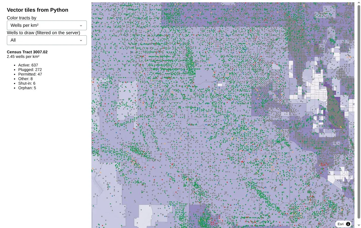
The tile only needs to carry the tract's ID and a few display fields. Python runs the spatial join for the details, which here is the count of wells inside the clicked tract, by status. The hook reaches the MapLibre map through a Plotly internal (gd._fullLayout.map._subplot.map), so pin your Plotly version if you copy it. The screenshot below shows the wells app after a click on a tract.
Step 7: 3D columns from tiles
MapLibre's fill-extrusion layer turns any polygon in a tile into a 3D block, with the height taken from a feature property. Extruding census tracts looked like buildings the size of states, because tracts vary so much in size. Shapes of the same size read much better, so we count wells per H3 hexagon, serve coarse hexagons when zoomed out and fine ones when zoomed in, and shrink each hexagon a little so the columns stand apart. Heights scale with the square root of the count, which keeps a handful of very dense fields from flattening everything else. In the wells app this is a third view, next to the tracts and wells, chosen with a radio button in the sidebar:
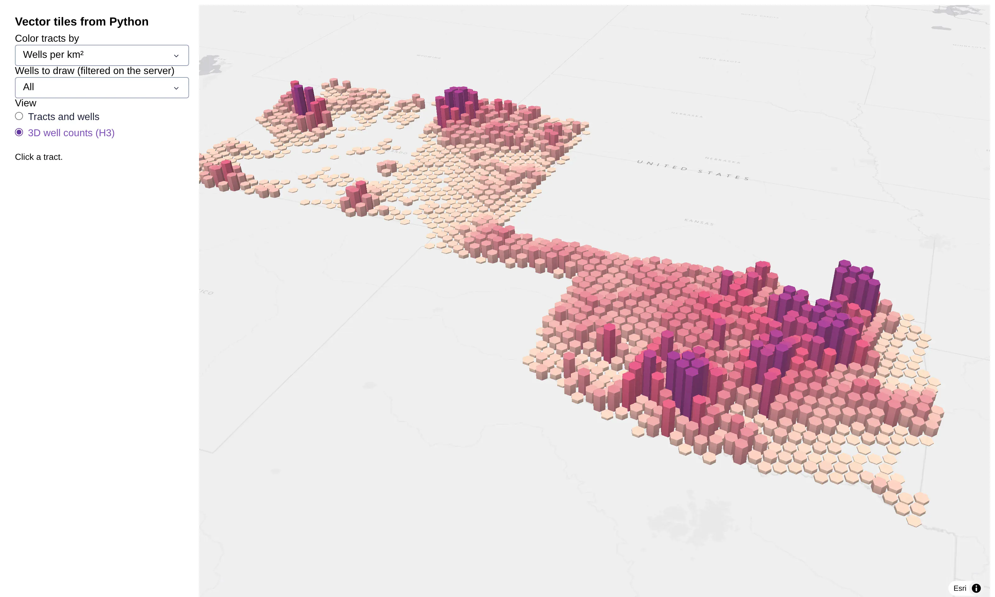
The heights are capped at the 99th percentile hexagon (3,822 wells at resolution 5), so the 15 hexagons above it are all drawn at the same full height. The well count here is from the state files as we downloaded them on November 4, 2026, which is a little higher than the 566,902 in the rest of this post because both states keep adding records.
Prompt: Count wells per H3 hexagon at resolution 5 and 7, shrink each hexagon to 82% of its size, and scale the height by the square root of the count against the 99th percentile, capped at 1. Save the hexagons as GeoParquet, serve them from the same tile route as a hexes layer (resolution 5 below zoom 8, resolution 7 above), and add a radio button that switches the map to a fill-extrusion layer of the hexagons with the map tilted to a pitch of 55.
This will create code like this:
import h3, numpy as np, pandas as pd, shapely, geopandas as gpdfrom shapely import affinityparts = []for res, max_height in [(5, 80_000), (7, 12_000)]: # meters; resolution 7 hexagons are about 7x narrowercounts = wells[f"h3_{res}"].value_counts() # wells per hexagon, from h3.latlng_to_cell(lat, lon, res)# square root against the 99th percentile, capped at 1, so a few huge fields don't flatten the restrel = np.minimum(1, (counts / counts.quantile(0.99)) ** 0.5)polys = [affinity.scale(shapely.Polygon([(lng, lat) for lat, lng in h3.cell_to_boundary(c)]), 0.82, 0.82)for c in counts.index] # shrink each one so the columns stand apartparts.append(gpd.GeoDataFrame({"res": res, "wells": counts.values, "rel": rel.values,"height": rel.values * max_height}, geometry=polys, crs=4326))pd.concat(parts).to_parquet("data/hexes.parquet") # loaded into DuckDB like the tracts, with an R-tree# in the tile function: one more layer, coarse hexagons below zoom 8 and fine ones abovesql = TILE_SQL.format(cols="wells, rel, height", layer="hexes", geom="geom", extent=4096, buffer=64,distinct="", where=f"AND res = {5 if z < 8 else 7}")HEX_LAYER = {"id": "hexes", "type": "fill-extrusion", "source": "hexes", "source-layer": "hexes","paint": {"fill-extrusion-height": ["get", "height"], "fill-extrusion-opacity": 0.9,"fill-extrusion-color": ["interpolate", ["linear"], ["get", "rel"],0, "#fde0c5", 0.6, "#d6456b", 1, "#7a1f6b"]},}fig.update_layout(map_pitch=55)
The same technique scales to several layers in one map: the hydrology app later in this post serves 87,028 subwatersheds, 712,768 river reaches and 8,082 stream gauges from one Python process.
How do you make vector tiles fast?
A working tile server and a fast one are a few small changes apart. To see what each change is worth, we timed the tile query on its own, without HTTP or caching, for the 3 by 3 block of tiles around central Oklahoma, which is the densest part of the well data. We added one change at a time and ran the same tests on DuckDB 1.5.6 and PostGIS 3.4 on a 4-vCPU cloud machine in October 2026. The hydrology app later in this post was measured on DuckDB 2.0, and the section after it covers what changed between the two versions. The two tables below show the results for the wells app's two layers, the census tracts and the wells.
Census tracts (84k polygons)
Slowest zoom 4 tile
Median zoom 10 tile
Average zoom 4 tile
Obvious SQL: index present, but a filter hides it
8.0 s
4.8 s
920 KB (382 KB gzipped)
Index actually used
4.1 s
5.9 ms
919 KB (381 KB gzipped)
Plus simplified geometry for low zooms
2.6 s
6.1 ms
548 KB (208 KB gzipped)
Plus dropping polygons smaller than a pixel
1.1 s
5.0 ms
195 KB (87 KB gzipped)
All of the above in PostGIS
66 ms
1.4 ms
211 KB (90 KB gzipped)
Wells (567k points)
Slowest zoom 4 tile
Median zoom 10 tile
Average zoom 4 tile
Every point
2.2 s
63 ms
2.7 MB (673 KB gzipped)
One point per pixel below zoom 10
665 ms
68 ms
29 KB (10 KB gzipped)
One point per pixel, PostGIS
895 ms
11 ms
29 KB (10 KB gzipped)
Make sure the spatial index is used
Clipping a shape to a tile can leave nothing behind, so the natural query wraps the clipped rows in WHERE geom IS NOT NULL. DuckDB's optimizer pushes that filter into the table scan and merges it with ST_Intersects, and the merged filter can't use the R-tree, so in our census tract layer a zoomed-in tile containing four tracts took 4.8 s, slower than the same table with no index at all (34 ms).
There are two fixes. On DuckDB 1.5.6 we put the clipping step in a MATERIALIZED CTE, as in Step 1, which stops the optimizer from moving the filter: DuckDB does the index lookup first and filters the clipped rows afterwards, and the same tile took 5.9 ms. The simpler fix is to leave the filter out, because ST_AsMVT skips NULL geometries on its own, and that's what the hydrology app does on DuckDB 2.0. You can check your own queries with EXPLAIN: on DuckDB 2.0 the plan should show an Rtree Index Scan under the filter (older versions print RTREE_INDEX_SCAN), and a Seq Scan means the index isn't being used. PostGIS plans the original query correctly without any changes.
We recommend the DuckDB 2.x series, which is a long-term support release with support promised until at least October 2027. The tile functions and their arguments are the same as in 1.5, so the queries in this post run on either, and on 2.0 the outer filter still slows tiles down the same way (a river tile went from 2.6 ms to 733 ms and a subwatershed tile from 7.8 ms to 49.3 s). Run EXPLAIN on your tile query again after each DuckDB upgrade, since this is optimizer behavior that can change between versions.
Simplify geometry for low zooms
At zoom 4 a census tract is a few pixels across, yet its full outline can have hundreds of vertices. Keeping a second geometry column that's simplified to about a pixel, and reading it at low zooms, saves most of that work.
Prompt: Add a second geometry column to the tracts table, simplified to about a pixel at zoom 7, plus an area column. Below zoom 8, read the simplified column and skip tracts smaller than about 2x2 pixels.
This will create code like this:
CREATE TABLE tracts ASSELECT *,ST_SimplifyPreserveTopology(geom, 1000) AS geom_lo, -- about a pixel at zoom 7ST_Area(geom) AS area_m2FROM (...);-- in the tile query, below zoom 8:-- read geom_lo instead of geom, and add AND area_m2 > 4e6 (about 2x2 pixels)
The average zoom 4 tile went from 919 KB to 548 KB. ST_SimplifyPreserveTopology keeps each polygon valid, and simplifying to about a pixel keeps any gaps between neighbors smaller than the eye can see at that zoom. Give the simplified column its own R-tree index too, since the low-zoom tiles filter on it.
Drop polygons smaller than a pixel
Most of the 84,000 tracts in the wells app are small urban ones, and at zoom 4 they show up as specks that still cost bytes. Skipping anything under about 2 by 2 pixels brought the tile down to 195 KB, and the rendered map looks the same. tippecanoe does the same thing by default when it builds tiles. Use an area column for this rather than setting the geometry to NULL: on DuckDB 1.5.6 we saw NULLs in an R-tree-indexed geometry column come back as corrupt blobs from the index scan.
Thin points when zoomed out
Points have the opposite problem. In our wells layer, a zoomed-out tile over Oklahoma contains hundreds of thousands of wells, which came to 2.7 MB per tile. Below zoom 10 you can encode the tile on a 256-unit grid, where one unit is one screen pixel, and keep a single point per grid cell.
Prompt: Below zoom 10, encode the wells tile on a 256-unit grid and keep one well per grid cell with DISTINCT ON.
This will create code like this:
-- below zoom 10: a 256-unit grid instead of 4096, then one point per grid cellSELECT ST_AsMVT(t, 'wells', 256, 'geom') FROM (SELECT DISTINCT ON (ST_X(geom), ST_Y(geom)) * FROM clipped WHERE geom IS NOT NULL) t
That tile drops to 29 KB and looks identical on screen. From zoom 10 up, every well is included. If the browser filters points by a property, add that property to the DISTINCT ON so each pixel keeps one point per value and the filter still shows every pixel that should be lit.
Compress, cache and use threads
Vector tiles compress 2 to 4 times with gzip, so compress each tile body. An lru_cache (Python's built-in least-recently-used cache) on the tile function means panning back over the same area costs nothing, and a Cache-Control header lets the browser keep tiles it has already seen. A map requests 10 to 30 tiles at once, and one process with many threads handles them best, because the threads share the DuckDB tables in memory where separate processes would each need their own copy.
Prompt: Add a gunicorn config that runs one worker process with 16 threads.
This will create code like this:
# gunicorn.conf.py: one process, many threads. A map asks for 10 to 30 tiles at once,# and threads share the DuckDB tables instead of copying them per process.workers = 1worker_class = "gthread"threads = 16
A bigger example: every watershed, river and stream gauge in the lower 48
Real map services carry more than two layers, so the hydrology app is built on US hydrology, the kind of base map that water, energy and insurance teams put under almost everything else. It has three layers. The first is all 87,028 HUC12 subwatersheds of the lower 48 (the smallest of the USGS watershed levels, each named by a 12-digit hydrologic unit code) from the USGS Watershed Boundary Dataset, shaded by where their water reaches the sea, which we worked out by following each subwatershed's downstream neighbor to the end of the chain. The second is 712,768 river reaches from NHDPlus V2.1, the national stream network from the EPA and USGS. It includes every stream of order 3 and up, where a stream with no tributaries is order 1 and the order goes up by one where two streams of the same order meet, and wider lines mean a higher order. The third is 8,082 active USGS stream gauges from the USGS National Water Information System (NWIS), colored by how their latest reading compares with the same day in past years, the way USGS WaterWatch does it. The data was retrieved on November 4, 2026, and 33,798 of the subwatersheds, 34.9% of their combined area, drain to the Mississippi.
Sent as GeoJSON, those three layers are 1.3 GB (339 MB gzipped), mostly because the subwatershed outlines alone have 40 million vertices. As vector tiles, the first view of the lower 48 took 12 tiles and 427 KB gzipped, the figure itself was 9.5 KB of JSON with no geometry in it, and zooming into the confluence of the Mississippi and the Ohio at Cairo, Illinois fetched 12 more tiles and 140 KB. The app runs the same queries on DuckDB 2.0 or PostGIS 3.4, chosen by one environment variable, and every timing in this section is from DuckDB 2.0. The recording below walks through the app from the first view to a zoomed-in click.
Prompt: Build a Dash app that serves US hydrology as vector tiles. Download the HUC12 subwatersheds from the USGS Watershed Boundary Dataset national file geodatabase, NHDPlus V2.1 flowlines of stream order 3 and up from the EPA's NHDPlus ArcGIS REST map service in pages, and active stream gauges with their latest discharge and day-of-year percentiles from the USGS NWIS web services. Reproject everything to EPSG:4326 and EPSG:3857, save each layer as GeoParquet, and load them into a DuckDB file with an R-tree index on every geometry column, or into PostGIS when DATABASE_URL is set. Add a Flask tile route per layer with ST_AsMVT, and draw the layers in a Plotly map through a MapLibre style with layer toggles, a stream order slider, a gauge color switch, a basemap menu and an inspect card for clicked features.
The sections below show the main pieces of the code that prompt produces, each with a smaller prompt for that piece.
One tile query in two SQL dialects
The two dialects differ in only three places: the parameter markers, ST_AsMVTGeom wanting a BOX_2D in DuckDB (hence ST_Extent), and the bounding box operator && that PostGIS uses for its GiST index where DuckDB uses ST_Intersects for its R-tree. The app keeps both side by side and picks one at startup:
Prompt: Write the tile query as a template for both DuckDB and PostGIS, with layer, columns, geometry column, table and an extra WHERE clause filled in per layer. Use $z/$x/$y and ST_Extent for DuckDB, %(z)s and && for PostGIS, leave out any outer IS NOT NULL filter, and pick PostGIS when DATABASE_URL is set.
This will create code like this:
TILE_SQL = {"DuckDB": """SELECT ST_AsMVT(t, '{layer}', 4096, 'geom') FROM (SELECT {cols}, ST_AsMVTGeom({geom}, ST_Extent(ST_TileEnvelope($z, $x, $y)), 4096, 64, true) AS geomFROM {table} WHERE ST_Intersects({geom}, ST_TileEnvelope($z, $x, $y)) {where}) t""","PostGIS": """SELECT ST_AsMVT(t, '{layer}', 4096, 'geom') FROM (SELECT {cols}, ST_AsMVTGeom({geom}, ST_TileEnvelope(%(z)s, %(x)s, %(y)s), 4096, 64, true) AS geomFROM {table} WHERE {geom} && ST_TileEnvelope(%(z)s, %(x)s, %(y)s) {where}) t""",}DIALECT = "PostGIS" if os.environ.get("DATABASE_URL") else "DuckDB"
There is no outer WHERE geom IS NOT NULL and no CTE, which is the DuckDB 2.0 form of the index fix above. Each table stores its geometry in Web Mercator more than once, at full detail in geom and simplified to 500 m in geom_lo for zoomed-out tiles (the subwatersheds also get a 60 m geom_mid), and every geometry column has its own spatial index.
Per-zoom rules for each layer
A subwatershed is a few pixels wide when you look at the whole country and a few hundred pixels wide at a river confluence, so each layer gets a short list of tiers, and the query builder picks the last one whose first zoom is at or below the tile's zoom:
Prompt: Give each tile layer a list of zoom tiers (first zoom, table, geometry column, properties), and use the last tier at or below the tile's zoom. Use an overview table of subwatersheds dissolved by HUC8 (the larger watershed level above HUC12) and outlet below zoom 6, the 500 m and 60 m simplified columns up to zoom 10, and below zoom 8 only send river reaches above a minimum stream order for each zoom.
This will create code like this:
LAYERS = {# (first zoom, table, geometry column, properties in the tile)"watersheds": [(0, "watershed_overview", "geom", "outlet"), # dissolved by HUC8 and outlet(6, "watersheds", "geom_lo", "outlet"), # simplified to 500 m(8, "watersheds", "geom_mid", "huc12, name, outlet"), # 60 m(11, "watersheds", "geom", "huc12, name, outlet, area_km2")],"rivers": [(0, "rivers", "geom_lo", "stream_order"),(8, "rivers", "geom", "comid, name, stream_order, flow_cfs")],"gauges": [(0, "gauges", "geom", "condition, cond_rank, drainage_mi2"),(7, "gauges", "geom", "site_no, name, condition, cond_rank, percentile, drainage_mi2, flow_cfs")],}# below zoom 8, rivers tiles carry only the bigger streams: order 7 and up at zoom 3 and 4, 6 at zoom 5, ...MIN_ORDER = {0: 8, 1: 8, 2: 8, 3: 7, 4: 7, 5: 6, 6: 5, 7: 4}
Zoomed out, a tile carries only the columns the style needs to draw it, and the map only draws subwatershed fills there, not outlines. That's why the zoomed-out tiers read a fourth table, the 87,028 subwatersheds dissolved into 2,425 shapes by HUC8 (the next watershed level up, with an 8-digit code) and outlet, which look the same once each one is filled with its outlet's color. For the 3 by 3 block of zoom 4 tiles around the confluence, the dissolved table cut the average subwatershed tile from 449 KB gzipped to 19 KB and the slowest one from 2,955 ms to 104 ms, and at zoom 9 the 60 m column cut the median tile from 43.0 ms to 17.6 ms. Rivers do the same with stream order, which is how every hydrography map handles scale: the Mississippi below the Missouri confluence (stream order 10) is in every tile, and the 323,143 reaches of order 3 only from zoom 8.
Two smaller DuckDB details came up while building this. ST_AsMVT in DuckDB 2.0 only encodes VARCHAR, FLOAT, DOUBLE, INTEGER, BIGINT and BOOLEAN properties, so a SMALLINT or TINYINT column fails the whole tile and needs a cast to INTEGER. And DuckDB 2.0 chose ZSTD compression for the full-detail subwatershed geometry, which made every row the R-tree found expensive to read back: the median zoom 11 subwatershed tile took 88.8 ms with ZSTD and 7.6 ms with it turned off (SET disabled_compression_methods = 'zstd' before creating the tables) at the cost of a bigger file (2.1 GB for all four tables). If a zoomed-in tile is slow while EXPLAIN shows the index in use, check the column's compression with pragma_storage_info.
How do you color vector tiles by value in a Plotly map?
There are two ways to put vector tiles on a Plotly map, and the difference shows as soon as you want the map to say something about the data. The simple one is layout.map.layers, where you add a tile URL as a layer. In Plotly 7.1, each of those layers draws every feature in one color, with no filter, which is fine for outlines like county borders. It can't make big rivers wider than creeks, color each stream gauge by how its flow compares with normal, or hide the smallest streams when someone moves a slider.
For that, you give layout.map.style a full MapLibre style document instead. It's the same JSON format that MapLibre and Mapbox maps use everywhere, with a sources entry for each tile route and a list of layers whose colors, widths and filters are expressions on each feature's properties (match for categories, step for classes, interpolate for smooth scales and for changing with zoom). Here's the same view of the hydrology app, where the Ohio River meets the Mississippi at Cairo, Illinois, drawn both ways:
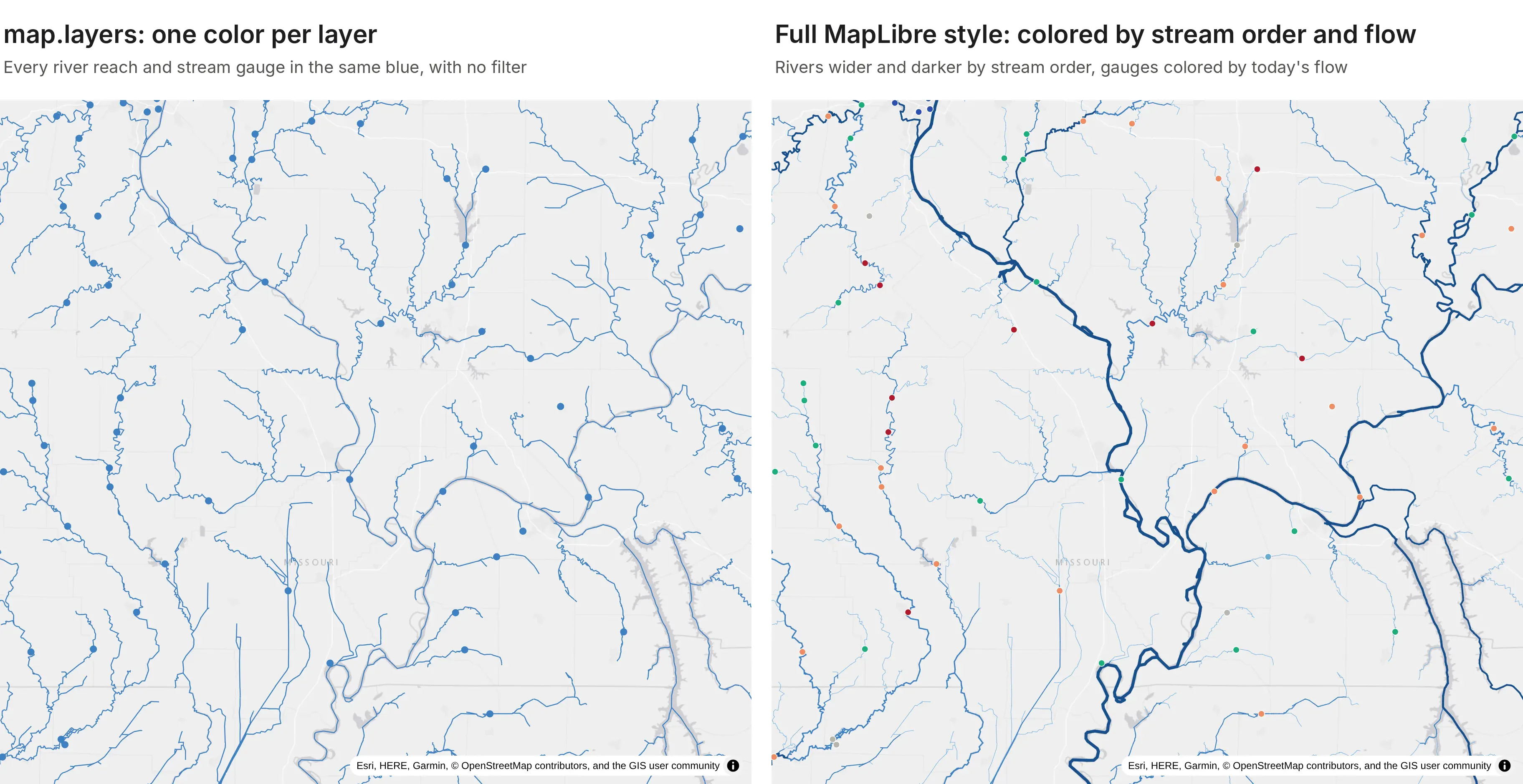
The style below is the one on the right. It also comes with a second benefit, explained after the code: because the styling happens in the browser, Dash controls can change it without fetching any new tiles.
Prompt: Build a MapLibre style dict for layout.map.style with an Esri light gray raster basemap and vector sources for the rivers and gauges tile routes with maxzoom 14. Draw rivers as lines filtered by the stream order slider, colored with a step expression and widened by stream order with a zoom interpolate, and gauges as circles colored with a match on their flow condition.
This will create code like this:
order = ["coalesce", ["get", "stream_order"], 3]style = {"version": 8,"sources": {"basemap": {"type": "raster", "tiles": [ESRI_LIGHT_GRAY], "tileSize": 256},"rivers": {"type": "vector", "tiles": [f"{origin}/tiles/rivers/{{z}}/{{x}}/{{y}}.pbf"], "maxzoom": 14},"gauges": {"type": "vector", "tiles": [f"{origin}/tiles/gauges/{{z}}/{{x}}/{{y}}.pbf"], "maxzoom": 14},},"layers": [{"id": "basemap", "type": "raster", "source": "basemap"},{"id": "rivers", "type": "line", "source": "rivers", "source-layer": "rivers","filter": ["all", [">=", order, 5], ["<=", order, 10]], # the stream order slider"paint": {"line-color": ["step", order, "#8ab8e0", 5, "#3d7fc1", 7, "#174f8c"],"line-width": ["interpolate", ["exponential", 1.6], ["zoom"],3, ["*", 0.12, ["^", ["-", order, 2], 1.25]],12, ["*", 0.75, ["^", ["-", order, 2], 1.25]]]}},{"id": "gauges", "type": "circle", "source": "gauges", "source-layer": "gauges","paint": {"circle-radius": ["interpolate", ["linear"], ["zoom"], 3, 1.6, 11, 6.5],"circle-color": ["match", ["get", "condition"], "Much below normal", "#b2182b","Below normal", "#ef8a62", "Normal", "#1baf7a", "Above normal", "#67a9cf","Much above normal", "#2a4fb0", "#b9b6ae"]}},],}fig.update_layout(map=dict(style=style, center=dict(lat=40.0, lon=-95.0), zoom=3.6))
The maxzoom of 14 on each source tells MapLibre to over-zoom the zoom 14 tile instead of asking the server for deeper ones. Every control in the app returns a Patch of the style's layers, or of the whole style for a basemap change. Moving the stream order slider, recoloring the gauges by drainage area, hiding a layer or switching the basemap sent 2.0 to 2.7 KB of JSON and caused no new vector tile requests, because MapLibre restyled the tiles it already had.
Clicking a feature: the nearest feature in SQL
We checked whether Plotly 7.1 sends hover or click events for features in a vector tile layer, drawn either through layout.map.layers or through a style dict. It doesn't: the gauges around the confluence rendered (8 features in view at zoom 9), but moving onto them and clicking them fired no plotly_hover or plotly_click, while an ordinary Scattermap point in the same figure fired both. Step 6 handled this by reading the clicked feature from the tile. The hydrology app does the other thing a GIS identify tool does: it sends the clicked position to Python and asks the database which feature is nearest.
Prompt: Plotly doesn't fire clickData for vector tile features. Add a clientside callback that hooks the MapLibre map inside the Plotly figure, sends the clicked lon, lat and zoom to a dcc.Store with set_props, and a Python callback that finds the nearest stream gauge or river within 8 pixels, or else the subwatershed under the click, with one SQL query per layer, shows its attributes and highlights it with a Scattermap trace.
This will create code like this:
NEAREST_SQL = """SELECT * EXCLUDE (geom, geom4326), ST_AsGeoJSON(geom4326) AS geojson,ST_Distance(geom, ST_Point($x, $y)) AS distFROM {layer}WHERE ST_Intersects(geom, ST_MakeEnvelope($x - $r, $y - $r, $x + $r, $y + $r))ORDER BY dist LIMIT 1"""def nearest(lon, lat, zoom, layers, px=8):x, y = to_3857(lon, lat)r = px * 2 * math.pi * 6378137.0 / (512 * 2 ** zoom) # 8 screen pixels in Mercator metersfor layer in ["gauges", "rivers", "watersheds"]: # top layer firstif layer in layers and (rows := db.rows(NEAREST_SQL.format(layer=layer), {"x": x, "y": y, "r": r})):return layer, rows[0]
The lookup for the Mississippi River gauge at Thebes, Illinois, in the screenshot at the top of this post took 7.8 ms in DuckDB, and it returns the 91 years of record behind that gauge's percentile, which the tile doesn't carry. Asking SQL also works at zoomed-out views where the tile holds only the columns needed to draw it.
Should you use DuckDB or PostGIS for vector tiles?
We timed the hydrology tile queries in both engines on the same three layers: the 3 by 3 block of tiles around the confluence at zooms 5, 7, 9 and 11, for every layer, which is 108 queries per pass, with the per-zoom tiers above. Times are for the SQL alone, on a 4-vCPU cloud container, with DuckDB 2.0 and PostGIS 3.4 on PostgreSQL 16.
Hydrology tile query time
DuckDB 2.0
PostGIS 3.4
First pass, median / 95th percentile
10.4 / 63.0 ms
2.9 / 40.5 ms
Warm, median / 95th percentile
10.0 / 68.1 ms
2.7 / 24.0 ms
Warm at zoom 5, median / 95th percentile
20.5 / 95.7 ms
6.0 / 151.8 ms
Warm at zoom 9, median / 95th percentile
13.1 / 23.3 ms
3.3 / 8.6 ms
Warm at zoom 11, median / 95th percentile
2.9 / 10.3 ms
0.7 / 3.3 ms
PostGIS had the lower median at every zoom, two and a half to four times lower, and was quickest on the polygon tiles (a warm median of 7.7 ms for subwatershed tiles against 20.1 ms in DuckDB). The exception was the zoomed-out river tiles, where PostGIS's slowest ones took longer (a 95th percentile of 133.3 ms against 91.4 ms in DuckDB), which is why its zoom 5 percentile is the higher one. The wells app's tuning tables on DuckDB 1.5.6 point the same way for polygons: PostGIS built a zoomed-in tract tile in 1.4 ms against 5.0 ms in DuckDB, and the slowest zoom 4 tile in 66 ms against 1.1 s, so 3.6 to 16 times faster. Points were closer, and the slowest thinned zoom 4 wells tile was faster in DuckDB (665 ms) than in PostGIS (895 ms). The two benchmarks ran on different DuckDB versions and data, so compare engines within a table rather than across them.
Both are fast enough that the browser's tile requests, not the database, set the pace once a cache sits in front. DuckDB has nothing to run, since it lives inside the Python process and reads GeoParquet directly. Use it when the data is a few GB and belongs to one app, and PostGIS when the data is shared between apps, updated continuously, or already lives there. The SQL carries over almost line for line, so you can start in DuckDB and move a layer later.
How do vector tiles compare with other ways to draw big maps in Dash?
The maps at scale post times every way we know to draw a large map in a Dash app, across Plotly, deck.gl, dash-leaflet and dash-openlayers, on the same layers. Its headline for tiles is that vector tiles in a Plotly map drew all 566,902 Oklahoma and Colorado wells from the wells app in 1.7 s, where a Plotly Scattermap of the same wells took 19.6 s, and drew about 84,000 census tracts in 1.9 s. Because the route speaks standard MVT, other clients can read it too: the community dash-openlayers component drew the same tracts from these tiles in 1.4 s. That post also covers when deck.gl is the better pick.
How do you deploy a Dash app that serves its own vector tiles?
A tile-serving app deploys like any other Dash app. Dash Enterprise runs it inside your own cloud account or data center, next to your PostGIS database and behind your company's login, which is usually what an ArcGIS Server replacement needs. Plotly Cloud is the quickest way to share one. A few settings mattered for both examples:
- Keep the DuckDB file on the persistent filesystem. Both platforms mount a persistent directory and set DASH_DATA_DIR. Store the database there, and the tables and R-tree indexes are built once, then reused every time the app restarts or redeploys.
- Build data in a background thread. Loading GeoParquet and building indexes at import time can take long enough that a small container misses its first health check. Start the build in a thread and have the tile function wait for it.
- Use the gunicorn.conf.py from the caching step and build tile URLs from the Origin header, as in Step 3.
- Size DuckDB from the container's memory. The wells app sets memory_limit to 400 MB to leave room in a 1 GB container.
- Write import flask, not from flask import request. A module-level request proxy makes the worker fail to start with "Working outside of request context".
Prompt: Store the DuckDB database in DASH_DATA_DIR so the tables and indexes are built once and survive restarts.
This will create code like this:
import osfrom pathlib import Path# Dash Enterprise and Plotly Cloud mount a persistent directory and point DASH_DATA_DIR at itDATA_DIR = Path(os.environ.get("DASH_DATA_DIR", "data"))con = duckdb.connect(str(DATA_DIR / "tiles.duckdb"))# build the tables and R-tree indexes once; later restarts open the file and skip thisif not con.execute("SELECT count(*) FROM duckdb_tables() WHERE table_name = 'tracts'").fetchone()[0]:build_tables(con)
Summary
Serving vector tiles from Python takes one Flask route and one ST_AsMVT query per tile, in DuckDB or PostGIS, and a Plotly map in Dash draws them through a MapLibre style so the browser only holds what's on screen. That's what lets a Dash app replace an ArcGIS map service for layers like the 566,902 oil and gas wells in the wells app or every subwatershed, river and stream gauge in the lower 48. Most of the speed comes from keeping the spatial index in use (on DuckDB, no outer IS NOT NULL filter, checked with EXPLAIN, and no ZSTD on big geometry columns), simplified geometry for low zooms, dropping what's smaller than a pixel, thinning points and caching gzipped tiles. For how tiles compare with deck.gl and the other map libraries, see Maps at scale in Dash, and for every other kind of map, the Python maps guide.