
Chris Parmer
2026-11-03
Maps at Scale in Dash: How to Make Large Plotly Maps Fast
TL;DR
- We timed every way to draw a large map in Dash on the same real data: 566,902 oil and gas wells from public Oklahoma and Colorado records, about 84,000 US census tracts and a national dataset of 52,244 lines. The numbers below come from that benchmark, which this post walks through.
- Up to about 100,000 points or a few thousand polygons, use Plotly's map traces (Scattermap, Choroplethmap), which give you hover, click, lasso and legends that crossfilter with the rest of a Dash app. In our example, we drew 100,000 of the wells in 3.7 s; all 566,902 took 19.6 s, and 2 million points (the wells plus jittered copies) ran the browser tab out of memory.
- For bigger layers, serve vector tiles from DuckDB or PostGIS and draw them inside the Plotly map. In our example, we drew all 566,902 wells in 1.7 s and all 84,000 census tracts in 1.9 s this way, and the cost stays about the same as the table grows.
- When every point has to stay in the browser and clickable at every zoom, use deck.gl through the community deckgl-dash package with binary arrays. In our example, it drew all 566,902 wells in 3.1 s, against 11.7 s for the same layer sent as JSON records.
- Keep geometry out of callbacks. In our choropleth of all 3,144 US counties, loading the GeoJSON by URL took the choropleth from 14.5 s to 4.4 s, and recoloring it with Patch() (Dash's partial update, which sends only the values that changed) sent 15 KB instead of 22.0 MB. We drew the 52,244 lines in 4.3 s with Plotly's map.layers by URL, while the same GeoJSON inside map.layers didn't finish in any of three runs.
- For drawing, editing and measuring geometry, use dash-leaflet, whose EditControl returns shapes to Python as GeoJSON.
This post tests drawing large maps like these in Dash, built on public data and timed in one benchmark app:
Points: all 566,902 oil and gas wells in the public Oklahoma Corporation Commission and Colorado Energy and Carbon Management Commission (ECMC) records, drawn five ways with the same filters. Here the page is set to deck.gl, a GPU map library:
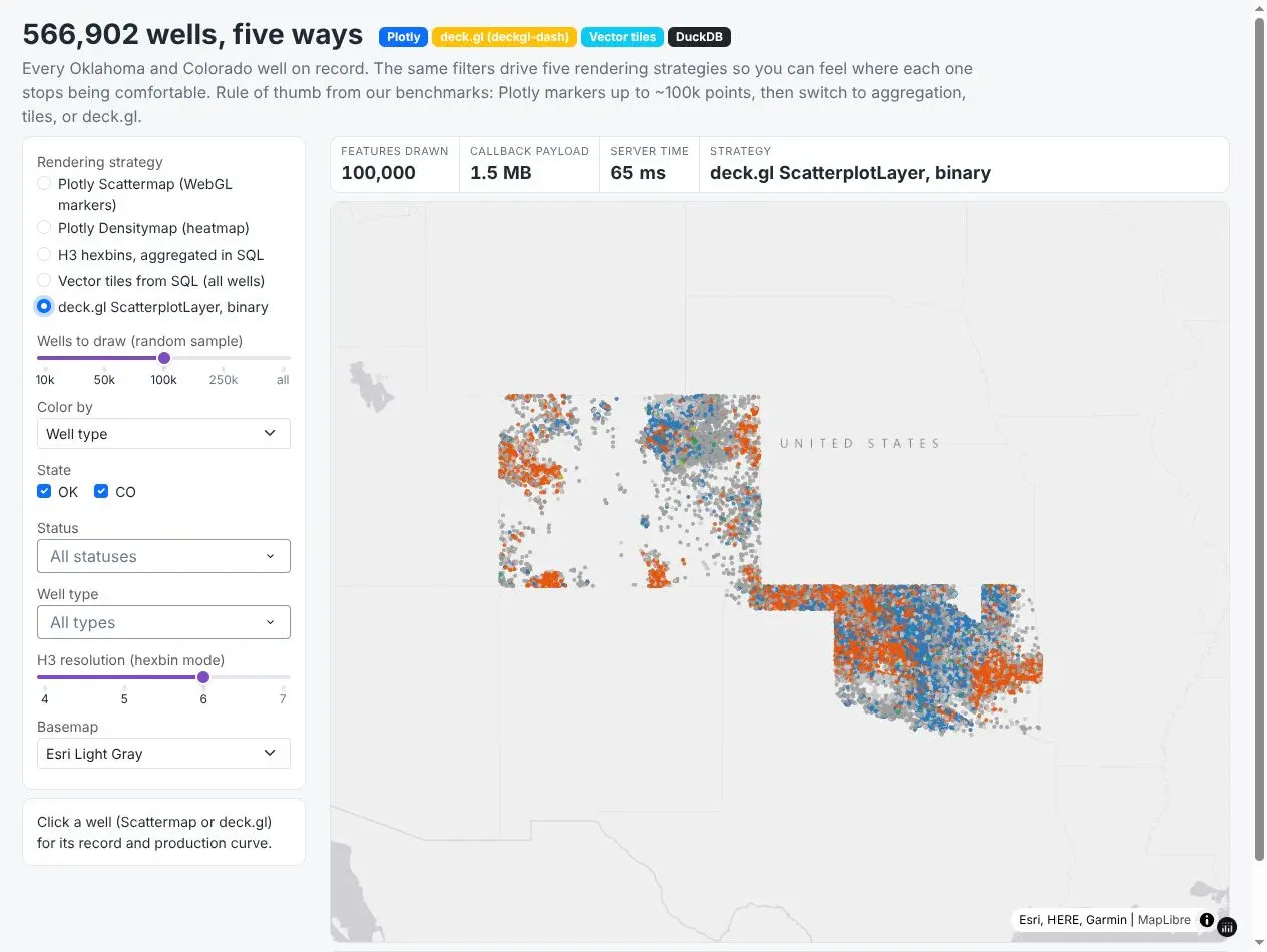
Prompt: Build a Dash page that draws the oil and gas wells from the Oklahoma Corporation Commission's RBDMS well data CSV and the Colorado ECMC wells shapefile five ways, chosen from a sidebar: a Plotly Scattermap, a Densitymap, H3 hexagons, vector tiles from DuckDB and a deckgl-dash ScatterplotLayer with binary arrays. Use the same operator and status filters on each, and show the callback payload size and server time in a panel.
Polygons: all 3,144 US counties and 84,121 census tracts from the Census Bureau's 2023 boundaries, shaded by the wells in each. The counties are a Plotly Choroplethmap, and the tracts, with 2.3 million vertices, are vector tiles:
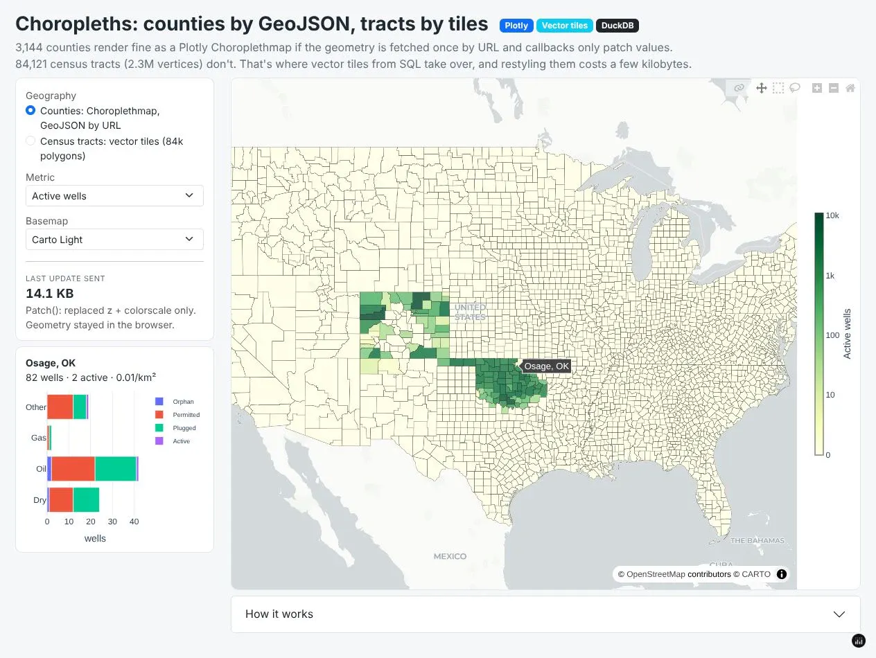
Prompt: Build a Dash page with the 2023 Census cartographic boundary counties and census tracts, shaded by the number of wells from our wells table in each. Draw the counties as a Plotly Choroplethmap with the GeoJSON served from a Flask route by URL and recolored with Patch(), draw the tracts as vector tiles from DuckDB, and show a detail panel with the wells by type and status for the clicked county.
Live services: one Plotly map of Houston that combines flood zones, radar and stream gauges from four public ArcGIS and OGC (Open Geospatial Consortium) web services, which the ArcGIS section further down shows how to build:
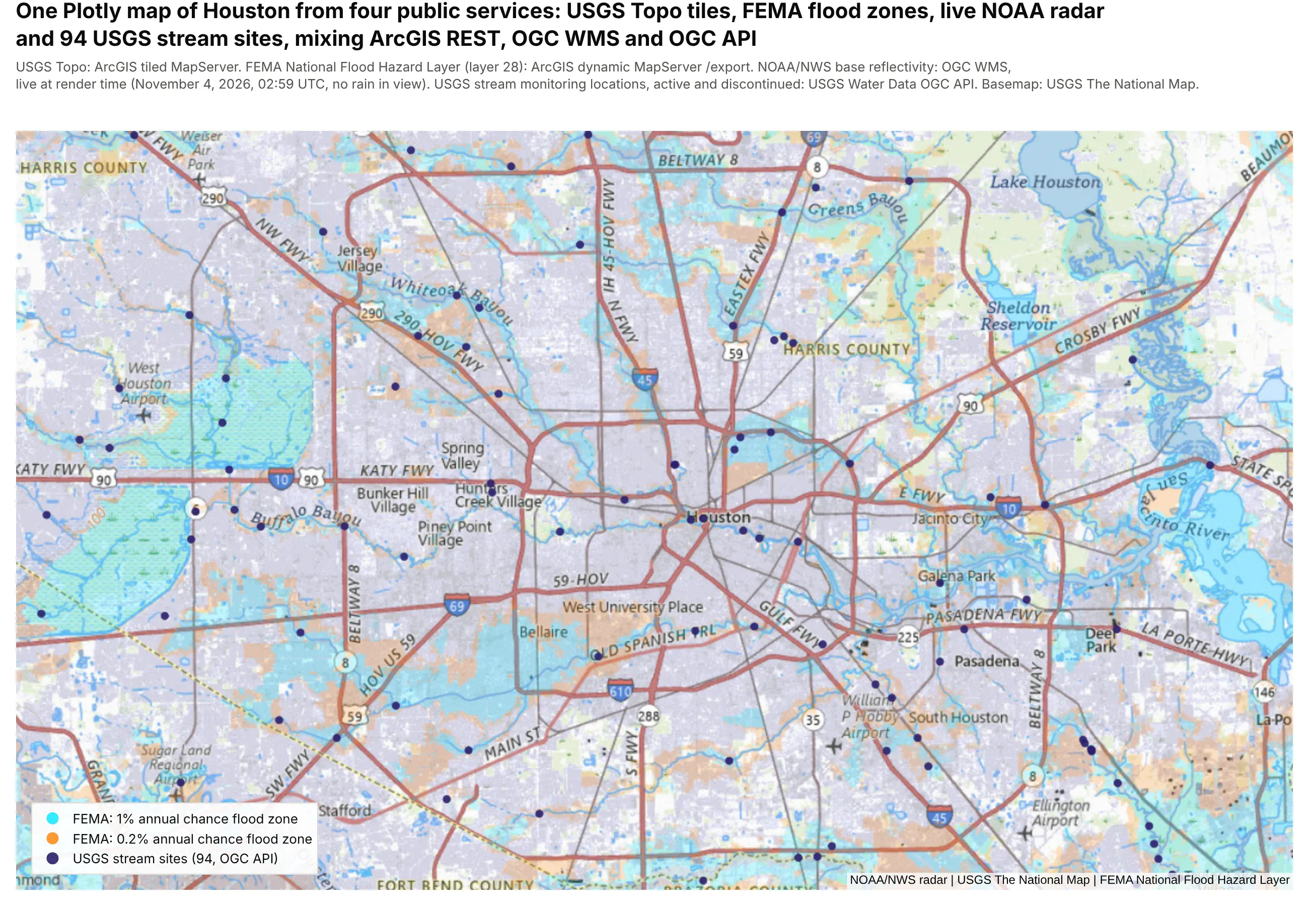
Prompt: Make a Plotly map of Houston in Python on the USGS Topo tiles from basemap.nationalmap.gov. Add the flood hazard zones from FEMA's National Flood Hazard Layer (NFHL, MapServer layer 28) as a raster source from the dynamic MapServer's /export endpoint with bbox={bbox-epsg-3857} and dpi=10, NOAA's radar mosaic over WMS, and the USGS stream monitoring sites from the USGS Water Data OGC API as a Scattermap trace, with a legend for each layer.
A lot of the oil and gas operators and utilities we work with are moving their maps off Esri and Spotfire, usually because their analysis already lives in Python and they want the maps next to it. The maps they need to move are big, since a Spotfire well map for one operator might hold every well in a basin, a utility's planning map has every census tract in its service territory, and both teams keep live layers from the ArcGIS Server they haven't switched off yet. Those maps also carry habits people rely on, like marking a few wells in Spotfire and watching every other chart follow, or opening an ArcGIS layer that stays quick at any zoom because the server only sends what's on screen.
Dash can do all of that, but there are several ways to draw a map in a Dash app and they behave very differently once a layer reaches tens of thousands of features. So we built the Dash app shown above on real public data from that world (every well record in Oklahoma and Colorado, every US census tract, a national dataset of 52,244 lines, and live ArcGIS, FEMA and NOAA services), timed every library and technique we could think of on the same layers, and wrote down what we'd recommend. This post is the performance deep dive in our Python maps guide, which covers making every kind of map in Python. Building vector tiles has its own post, vector tiles in Python from DuckDB or PostGIS, so this one only summarizes their benchmark results.
What kinds of maps did we test?
Most large maps in these teams' work are made of three kinds of layer, so we tested one of each, at the size they work with:
- Points: the 566,902 Oklahoma and Colorado wells in the first screenshot above, the kind of asset map an operator keeps open all day. The app draws them as Plotly markers, a density map, H3 hexagons (Uber's hexagonal grid for counting points by area), vector tiles and deck.gl.
- Polygons: the counties and census tracts in the second screenshot, the kind of layer a planning map or a market map is built on.
- Lines: 52,244 lines from a public national dataset, plus a smaller network of 33,087 segments, the size of a regional network map. The lines chart further down has their timings.
Which map library should you use in a Dash app?
Dash apps can draw maps with Plotly's own map traces or with one of four community libraries, all open source. They wrap different JavaScript map engines, which is why they reach different sizes:
Library
Built on
What it adds
Plotly map traces (Scattermap, Choroplethmap, Densitymap)
MapLibre GL (WebGL)
Hover, click and lasso events, legends, partial updates with Patch(), and crossfiltering with every other Dash component. layout.map.style takes any MapLibre style, so the same map can also draw vector tiles and raster services
Leaflet
Drawing and editing geometry, measuring, WMS layers, a classic layer control and fast marker clustering
deck.gl 9 (WebGL)
GPU layers for millions of points, arcs, 3D columns and heatmaps, with binary data transport. It replaces Plotly's original dash-deck, which hasn't been updated since its 0.0.1 release in 2020 and can't load in the same app
OpenLayers
OGC services, map projections, editing tools and fast vector tile rendering
Leaflet 2
An early look at Leaflet 2 for Dash 4, with pointer events for touch and stylus and map rotation
Underneath them are a few technologies worth knowing by name, because they decide how big a map can get. GeoJSON is geometry written as JSON text: every library reads it, but large layers get big and slow to parse. Binary arrays and geobuf carry the same data compactly, and Plotly sends NumPy arrays as typed arrays automatically. Vector tiles (MVT) cut a layer into squares per zoom level so the browser only downloads what's on screen, and raster tiles are the pre-drawn images that basemaps, satellite imagery, ArcGIS MapServers and WMS services (the OGC standard for serving map images) send. GeoParquet is the columnar file format for storing geometry on disk, which DuckDB reads directly. For drawing, SVG makes each feature a page element (fine up to a few thousand), canvas paints pixels with the CPU (tens of thousands), and WebGL hands the drawing to the GPU, which is how MapLibre, deck.gl and Plotly's map traces reach millions of vertices.
Which approach should you use for a large map?
Here's what we recommend for the maps we see most often in energy and utility work. The sections after the benchmarks go through each row with code.
What you're building
Approach
Why
A point map, up to about 100k points
Plotly Scattermap with NumPy arrays
Hover, click and lasso crossfilter with the rest of the app
A choropleth of counties or states
Plotly Choroplethmap, GeoJSON by URL, updates with Patch()
The geometry loads once, and recoloring sends a few KB
Census tracts, parcels or any layer of 10k+ polygons
Vector tiles from DuckDB or PostGIS in a Plotly map
The browser only loads what's on screen
Line networks such as rivers, roads and routes
Vector tiles, or a GeoJSON URL in map.layers for smaller networks
Full detail at any zoom
500k+ points that all stay visible and clickable
deckgl-dash with binary arrays
GPU rendering with compact data
"How many are there here?" at any scale
H3 aggregation in SQL, or clustering
A few thousand rows instead of the whole table
Drawing, editing and measuring geometry
dash-leaflet EditControl and MeasureControl
Shapes come back to Python as GeoJSON
Existing ArcGIS and WMS services
Raster sources in the Plotly map style, or dash-leaflet layers
Keep the services you already run
How we measured Dash map performance
Every number in this post comes from the same public data, with nothing synthetic in the benchmarked layers:
- 566,902 oil and gas wells: every well in the Oklahoma Corporation Commission RBDMS and Colorado ECMC databases. The 2 million point case is the same wells plus jittered copies, so it's the one partly synthetic layer, used only to see where each library breaks.
- 84,121 census tracts and 3,144 counties from the Census TIGER/Line 2023 cartographic boundaries.
- 52,244 lines from a public national line dataset (HIFLD) and a second, smaller network of 33,087 line segments from the US Energy Information Administration (EIA), both read from public ArcGIS feature services.
The benchmark itself is a second Dash app, separate from the one in the screenshots, that renders one map per URL through a real Dash callback, so the timing covers what a production app does: Python builds the component, Dash serializes it, and the browser draws it. Headless Chromium records how long each map took to be ready, measured from the callback request until the map was drawn, every network request had finished and the page had been idle for 1.5 s. "Drawn" was checked three ways (MapLibre's loaded() for Plotly, screenshots that stopped changing, and a minimum count of colored pixels), because deck.gl can fetch data in a worker while the screen is still blank. It also records the bytes sent, how long the main thread was blocked, the cost of one hover and the frame rate while panning.
There was no basemap, so only the data layer is timed. The machine was a 4-vCPU cloud container with no GPU, so WebGL ran on Mesa's llvmpipe software rasterizer. A laptop with a GPU is faster across the board, and the software rasterizer flatters the libraries that draw on the CPU (Leaflet) and penalizes the GPU ones, especially in frame rate. The comparisons between approaches are what carry over. Each case ran three times, and we report the median of the two warm runs (the first run builds server caches). One more number helps read the charts: an empty Plotly map took 1.6 s to be ready on this machine, against 0.2 to 0.6 s for the other libraries, so about 1.6 s of every Plotly bar is a fixed start-up cost that doesn't grow with the data.
Prompt: Write a benchmark for Dash maps: a Dash app that renders one map per URL through a real callback, for each library (Plotly Scattermap, Densitymap, Choroplethmap and vector tiles, dash-leaflet, deckgl-dash, dash-deck, dash-openlayers, dash-leaflet2) and each layer (the wells, census tracts and lines). Drive it with Playwright in headless Chromium, and for each case record the time from the callback request until the map is drawn, all requests have finished and the page has been idle for 1.5 s, plus bytes sent, main-thread blocking time, the cost of one hover and the frame rate while panning. Run each case three times and keep the median of the two warm runs.
How the approaches compare: points, polygons and lines
Points: 566,902 wells
The first benchmark drew every oil and gas well from the public Oklahoma and Colorado records as points, once per library and technique. The chart shows how long each took to be ready.
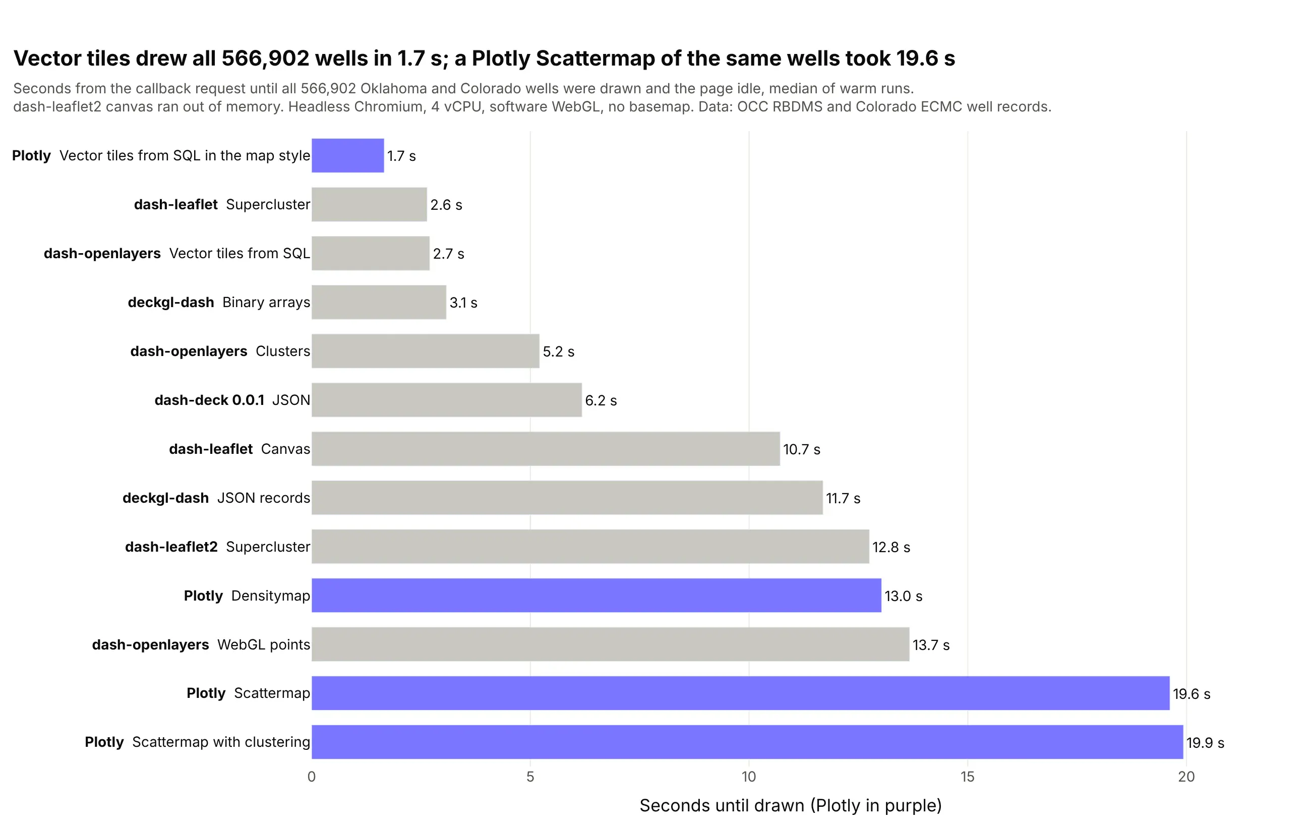
- Plotly's Scattermap is comfortable to about 100k points and slow well before 566k. When we drew 100,000 of the wells, the map was ready in 3.7 s, and one hover took about 64 ms. At 566,902 the map took 19.6 s and a hover about 370 ms, and at 2 million the browser tab ran out of memory. The time goes into JavaScript objects, because plotly.js turns every point into an object and then a GeoJSON feature before MapLibre draws it.
- Vector tiles draw the whole table at a cost that doesn't grow with the table. The browser asks only for the tiles in view, and a zoomed-out tile keeps one point per pixel, so all 566,902 wells were ready in 1.7 s after 87 KB crossed the network. The Scattermap callback for the same wells was 7.3 MB.
- deck.gl with binary arrays is the fastest way to keep every point in the browser. All 566,902 wells drew in 3.1 s from a 9.6 MB payload, and the main thread was blocked for only 77 ms. The same layer sent as JSON records took 11.7 s and 27.3 MB, so the data format matters as much as the library. With binary arrays, 2 million points drew in 11.1 s.
- Plotly's built-in clustering made large layers slower, not faster. At 100,000 points it took 6.2 s against 3.7 s without clustering. For clusters at this size, dash-leaflet's supercluster drew all 566,902 wells in 2.6 s and 2 million in 9.5 s, and kept panning at 60 frames a second, though you only ever see clusters.
Polygons: 84,000 census tracts
The second benchmark drew about 84,000 US census tracts from the Census TIGER/Line 2023 boundaries as filled polygons, the kind of layer a utility's planning map is built on.
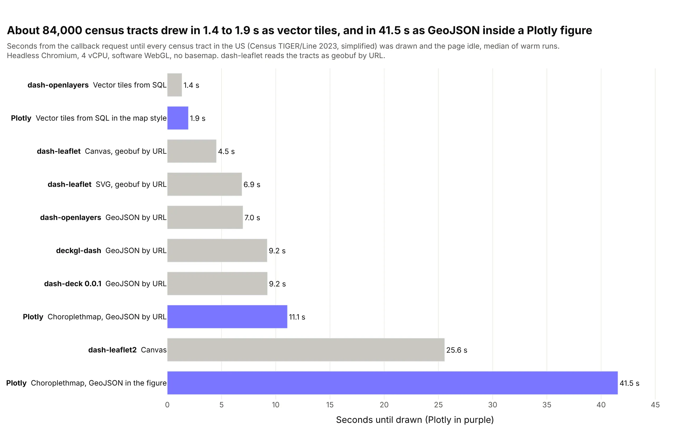
The chart uses the tracts simplified at build time, which is what we'd serve in an app. At full detail the order was nearly the same and the gaps were wider:
- GeoJSON inside the figure is the slowest choice for polygons. The simplified tract choropleth took 41.5 s with a 60.1 MB callback when the GeoJSON was in the figure, and 11.1 s when it loaded by URL. At full detail the in-figure version took 77.2 s and pushed 117.5 MB through one callback.
- Counties are fine in every library once the GeoJSON loads by URL. We also drew all 3,144 US counties from the same Census boundaries, and at full detail they were ready in 4.4 s in a Plotly Choroplethmap with a URL (14.5 s with the GeoJSON in the figure) and 1.6 s in dash-leaflet's canvas renderer reading geobuf.
- Vector tiles were the only approach that stayed under about 2 s for tracts. The Plotly map drew them in 1.9 s simplified and 2.1 s at full detail, and dash-openlayers in 1.4 s at both, because the first view only needs a few hundred kilobytes of tiles (769 KB on the wire) however detailed the table is.
- Leaflet held up well on mid-sized layers, then ran out of room. The canvas renderer drew simplified tracts in 4.5 s, but the page was frozen for 3.0 s of that, and at full detail the JavaScript heap reached 1.6 GB.
Lines: a national dataset of 52,244 lines
The third benchmark drew a national dataset of 52,244 lines, read from a public ArcGIS feature service.
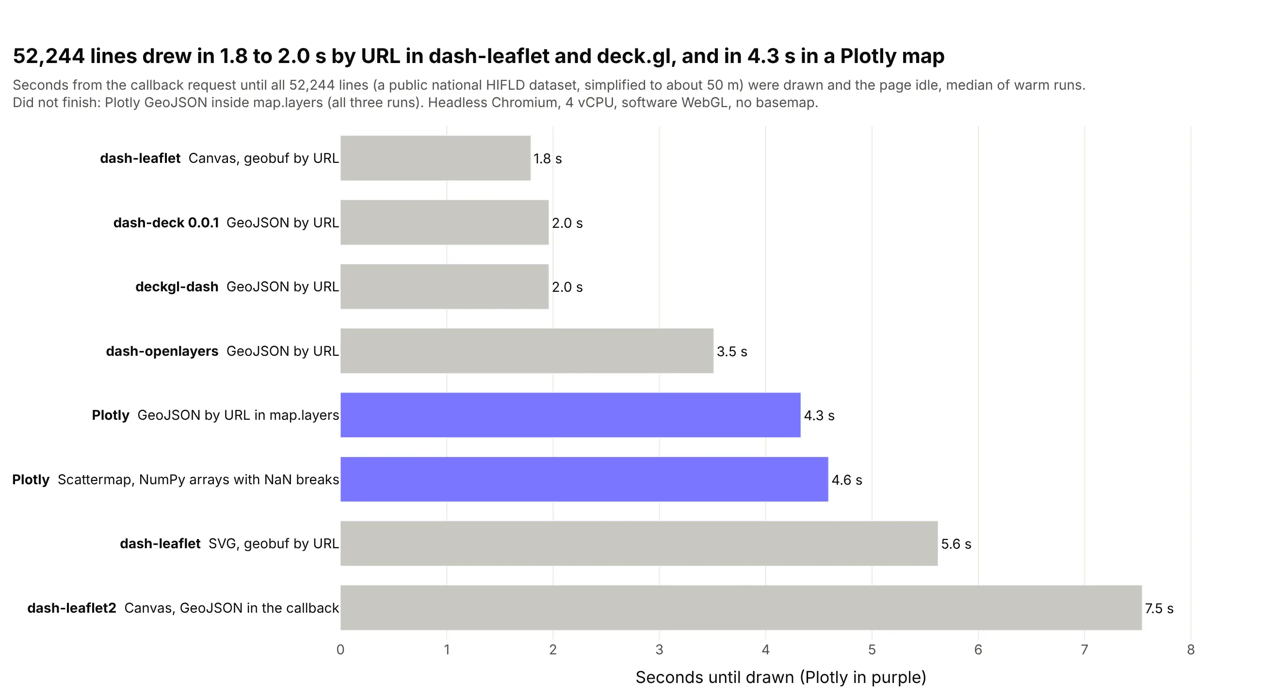
This chart uses the default case, every line simplified to about 50 m (GeoSeries.simplify(0.0005)), and we also ran the smaller 33,087-segment network and the 52,244 lines at full detail (1.87 million vertices):
- Never put a big GeoJSON inside layout.map.layers. Plotly's map with the 52,244 lines inline in map.layers didn't finish in any of three runs, and neither did the smaller 33,087-segment network. The same layers with source set to a URL drew in 4.3 s and 3.1 s. The cause is that plotly.js turns the whole source into a string to compare it on every update, which we're fixing.
- One Scattermap trace with NaN breaks is how you get hover and click on a line network, and it drew the simplified lines in 4.6 s from a 10.5 MB callback. Hover gets expensive with vertex count (about 240 ms per hover simplified and about 1 s at full detail, where the map took 15.6 s), so set hoverinfo="skip" on a full-detail layer and put the hover on a simplified copy.
- dash-leaflet's canvas renderer was the fastest at drawing lines, with 1.8 s simplified and 3.2 s at full detail, and panning stayed near 50 frames a second. The full network took the JavaScript heap to 684 MB, though, so it suits a page that shows one network rather than several.
- For a national line network at full detail, use vector tiles. Plotly and deck.gl both slowed down as the vertices grew (7.0 s and 5.5 s at full detail), while a tile only ever holds the lines in view.
How to make a fast choropleth map in Dash
For counties, states and other layers up to a few thousand polygons, Plotly's Choroplethmap is the right tool, as long as the geometry doesn't travel through your callbacks. Serve the GeoJSON from a Flask route with cache headers and pass its URL, so the browser fetches it once:
Prompt: Add a Flask route to my Dash app that serves counties.geojson gzipped with a one-day Cache-Control header, and draw it in a go.Choroplethmap by passing that URL as geojson instead of the GeoJSON itself.
This will create code like this:
@server.route("/geo/<name>.geojson")def geojson(name):resp = flask.Response(gzip.compress(geojson_bytes(name)), mimetype="application/geo+json")resp.headers.update({"Content-Encoding": "gzip", "Cache-Control": "public, max-age=86400"})return respgo.Choroplethmap(geojson="/geo/counties.geojson", locations=geoids, z=values, featureidkey="id")
In our benchmark, a choropleth of all 3,144 US counties at full detail took 14.5 s with the GeoJSON in the figure and 4.4 s with a URL. To change the colors after that, return a Patch() that replaces z and nothing else:
Prompt: Write a Dash callback that recolors the Choroplethmap when the dropdown changes by returning a Patch() that replaces only the trace's z values.
This will create code like this:
p = Patch()p["data"][0]["z"] = new_valuesreturn p
We recolored the counties, the census tracts and 100,000 of the wells in the benchmark app three ways, and here's what each cost from the click until the map was redrawn (median of five runs):
Update
Patch
Whole figure, GeoJSON by URL
Whole figure, GeoJSON inside
Recolor 3,144 counties
2.2 s, 15 KB
2.3 s, 66 KB
10.9 s, 22.0 MB
Recolor 84k tracts
8.2 s, 358 KB
8.7 s, 2.1 MB
35.3 s, 60.5 MB
Recolor 100k wells
2.0 s, 200 KB
2.2 s, 1.3 MB
n/a
Recolor 84k tracts as vector tiles
579 ms, 412 bytes
570 ms, 7 KB
n/a
The patch and the whole figure by URL cost about the same here because the geometry was already out of the callback, and what's left is plotly.js redrawing. A Choroplethmap rebuilds its geometry whenever z changes, which is why recoloring 84,000 tracts still took 8.2 s. The vector tile version keeps its colors in the map style's paint expressions, so MapLibre recolors the tiles it already has and nothing is fetched.
Two more tips for polygon layers. Simplify the geometry when you build the data: coverage-aware simplification (GeoSeries.simplify_coverage) took our Census county boundaries from 1.0 million to 228,000 vertices with no gaps between neighbors and no visible difference at state scale. And drop empty polygons before you serialize (gdf[~gdf.geometry.is_empty]). In our tract layer, simplification collapsed two tiny Manhattan tracts to empty polygons, and one empty polygon stops a Plotly map from drawing at all.
How many points can a Plotly map handle?
About 100,000 in a Scattermap, with full hover, click and lasso, and most operational well and asset maps fit in that range. Four habits keep it quick:
- Send NumPy arrays. Plotly serializes them as base64 typed arrays, and float32 coordinates are precise to about a meter at half the bytes of float64.
- Keep hover cheap. In our benchmark, hover strings for all 566,902 wells added about 12 MB to the figure. Put a row id in customdata, show a few numeric fields on hover, and look up the full record in a clickData callback.
- Send lasso selections as a polygon with a clientside callback (shown in the patterns section below), so Python never receives a list of 100,000 points.
- Aggregate when zoomed out. Tag every row with its H3 cell once (h3.latlng_to_cell), and "where are the wells?" becomes a GROUP BY that returns a few thousand hexagons.
Prompt: Draw the wells DataFrame in a go.Scattermap with lat and lon as float32 NumPy arrays, the row index in customdata for click lookups, and markers colored by status_code.
This will create code like this:
lat = wells.lat.to_numpy(np.float32)lon = wells.lon.to_numpy(np.float32)fig = go.Figure(go.Scattermap(lat=lat, lon=lon, mode="markers", customdata=wells.index.to_numpy(),marker=dict(size=5, color=wells.status_code, colorscale="Viridis")))
In our benchmark, recoloring 100,000 of the Oklahoma and Colorado wells with a Patch() of marker.color took 2.0 s and sent 200 KB. At 566,902 wells the same recolor crashed the browser tab, which is another sign that a layer that size belongs in tiles, deck.gl or an aggregate.
How to show every point on screen with deck.gl in Dash
Some maps need every one of hundreds of thousands of points drawn and clickable at once, such as a full well inventory for a state that an engineer filters by operator and status. That's what deck.gl is built for, and the community deckgl-dash package brings deck.gl 9 to Dash. Send the data as binary arrays:
Prompt: Draw the wells with deckgl-dash in Dash: a ScatterplotLayer with use_binary=True, positions as a float32 NumPy array of lon and lat, fill colors as an RGBA array, a 2-pixel radius and picking on, centered on Oklahoma.
This will create code like this:
from deckgl_dash import DeckGLfrom deckgl_dash.layers import ScatterplotLayerlayer = ScatterplotLayer(id="wells", use_binary=True, pickable=True, radius_units="pixels", get_radius=2,data={"getPosition": np.column_stack([lon, lat]).astype(np.float32), "getFillColor": rgba})DeckGL(id="deck", layers=[layer], initial_view_state={"longitude": -98, "latitude": 36, "zoom": 5})
The wells page shown at the top of this post draws them five ways with the same filters, so you can switch between them and feel the difference. Vector tiles drew all the wells faster than deck.gl did, because a zoomed-out tile keeps one point per pixel and the browser only holds the tiles in view. deck.gl keeps every well in the browser, so you can hover or click any one of them at any zoom, and filter or recolor all of them without a trip to the server. Pick deck.gl when that matters, and vector tiles when the table is too big to send at all.
dash-deck or deckgl-dash?
The Dash docs still point to dash-deck for deck.gl, but it's a 0.0.1 release from 2020 that bundles deck.gl 8.2.5 (deck.gl is now on 9.x) and takes data as JSON only. Some deck.gl and pydeck examples don't apply to it: radiusUnits="pixels" doesn't exist in 8.2, so a radius of 2 means two meters and the points vanish without an error (use radiusMinPixels instead). It drew every case in our benchmark once we accounted for that, and took 6.2 s and a 116 MB callback for all 566,902 wells. It also can't share a page with deckgl-dash, because deck.gl throws "multiple versions detected" and the second bundle never registers. For new work we'd use deckgl-dash, which is MIT licensed, maintained, and adds binary transport, MapLibre basemaps, drawing and a time filter.
When to use vector tiles in a Dash map
Every benchmark above has vector tiles at or near the top, and they're how ArcGIS serves big layers too. A vector tile layer is cut into a pyramid of square tiles, one set per zoom level, and each tile holds only the features inside it, simplified for that zoom, in the compact Mapbox Vector Tile (MVT) format. The browser downloads the tiles on screen and nothing else, so the size of the table stops mattering.
You don't need a tile server product to make them. DuckDB's spatial extension and PostGIS both have an ST_AsMVT function that builds a tile from a SQL query, so one Flask route in the Dash app (/tiles/<layer>/<z>/<x>/<y>.pbf) can serve tiles straight from a table. On the Plotly side, layout.map.style takes a full MapLibre style with a vector source pointing at that route, and the styling lives in MapLibre paint and filter expressions:
Prompt: Add my /tiles/tracts/{z}/{x}/{y}.pbf route to a Plotly map as a vector source in layout.map.style, with a fill layer colored by wells_per_km2 through a MapLibre interpolate expression.
This will create code like this:
style = {"version": 8,"sources": {"tracts": {"type": "vector", "tiles": [f"{origin}/tiles/tracts/{{z}}/{{x}}/{{y}}.pbf"]}},"layers": [{"id": "tracts", "type": "fill", "source": "tracts", "source-layer": "tracts","paint": {"fill-color": ["interpolate", ["linear"], ["get", "wells_per_km2"],0, "#f2f0f7", 1, "#7A76FF", 10, "#2a1f6b"]}}]}fig.update_layout(map=dict(style=style, center=dict(lat=38.5, lon=-96.5), zoom=3.6))
What they did in our benchmarks:
Layer
Vector tiles
Best non-tile approach
566,902 wells
1.7 s in a Plotly map, 2.7 s in dash-openlayers, 87 KB of tiles
deckgl-dash binary arrays, 3.1 s
84,121 tracts, simplified
1.9 s in a Plotly map, 1.4 s in dash-openlayers
dash-leaflet canvas, 4.5 s
84,121 tracts, full detail
2.1 s in a Plotly map, 1.4 s in dash-openlayers
dash-leaflet canvas, 6.4 s
Recolor 84,121 tracts
579 ms and 412 bytes, by patching the style
Choroplethmap with Patch(), 8.2 s
The trade-off is that features in a tile layer are drawn by MapLibre rather than by a Plotly trace, so Plotly doesn't send hoverData or clickData for them today, and styling is written as MapLibre expressions instead of Plotly's colorscales. The vector tiles post covers everything about building them: the tile SQL in both DuckDB and PostGIS, how to make tiles fast, filtering on the server by URL, a workaround for clicks on tile features, 3D hexagon columns and pre-built PMTiles files.
Patterns for large map apps in Dash
Most of the speed in a large map app comes from a few patterns that apply whichever library draws the map. Two of them, GeoJSON by URL and Patch(), are in the choropleth section above. These are the others.
Query by viewport
A viewport query sends the visible area to SQL on every pan and zoom, returning H3 hexagons when zoomed out and individual wells when zoomed in, so the browser never holds more than a screenful. That's how an ArcGIS feature service behaves. Plotly maps report their visible corners in relayoutData["map._derived"] (relayoutData is the property a Dash graph updates on every pan and zoom):
Prompt: Write a Dash callback that reads the visible corners from relayoutData["map._derived"], queries DuckDB for the wells in that box, and returns a Patch() with H3 hexagon counts below zoom 8.5 and individual wells above it.
This will create code like this:
@callback(Output("map", "figure"), Input("map", "relayoutData"))def load_view(relayout):corners = relayout["map._derived"]["coordinates"] # four [lon, lat] cornersw, s, e, n = bbox(corners)p = Patch()if relayout.get("map.zoom", 6) < 8.5:hexes = duck.execute("SELECT h3_6, count(*) AS wells FROM wells WHERE lon BETWEEN ? AND ? ""AND lat BETWEEN ? AND ? GROUP BY 1", [w, e, s, n]).df()p["data"][0] = hex_choropleth(hexes)else:p["data"][0] = well_points(w, s, e, n)return p
Our app has a page that runs this query on the Oklahoma and Colorado wells, with a panel that reports what each query returned. The screenshot shows it zoomed out over Oklahoma.
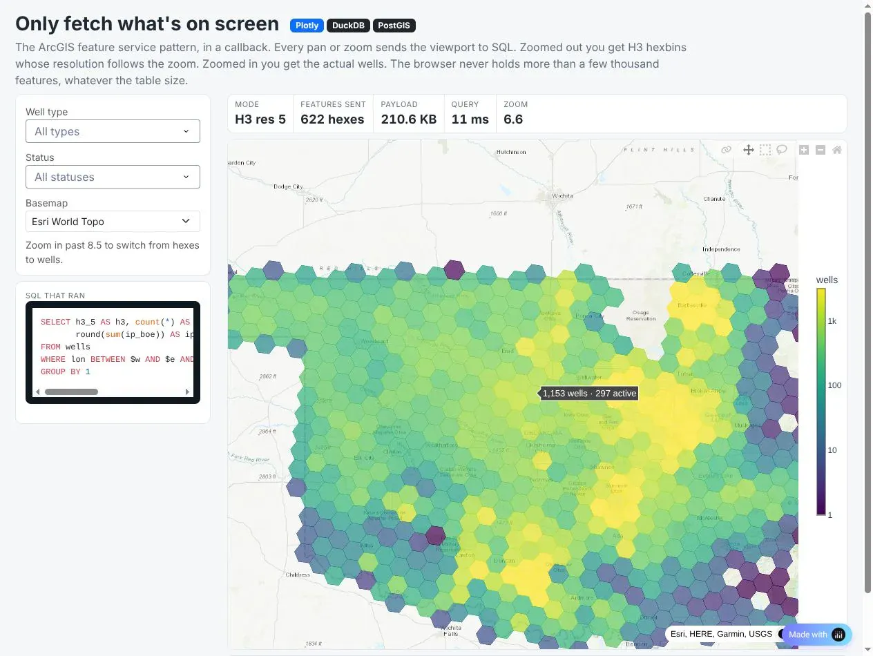
In the screenshot, the zoomed-out view of Oklahoma came back as 622 hexagons at H3 resolution 5, from an 11 ms query and a 210.6 KB payload. If you'd rather show clusters than hexagons, dash-leaflet's supercluster groups all 566,902 wells into bubbles in 2.6 s, and the bubbles split apart as you zoom in.
Prompt: Build a Dash page with a Plotly map of the wells that reruns a DuckDB query on every pan and zoom from relayoutData's map._derived corners. Below zoom 8.5 return H3 hexagon counts as a Choroplethmap, above it return the individual wells as a Scattermap, and show the H3 resolution, row count, payload size, query time and SQL in a side panel.
Selections as geometry
Spotfire users expect to mark rows on the map and have every chart and table follow, and Plotly's selectedData does that. The catch at scale is that a lasso around 50,000 wells puts 50,000 points in selectedData, so a clientside callback reduces it to the lasso polygon, and Python finds the wells inside it with one spatial query:
Prompt: Write a clientside callback that turns the map's selectedData into just the lasso polygon from lassoPoints.map and stores it in a dcc.Store, so Python runs one spatial query instead of receiving every selected point.
This will create code like this:
clientside_callback("(sel) => sel && sel.lassoPoints ? sel.lassoPoints.map : null",Output("lasso", "data"), Input("map", "selectedData"))
This operations dashboard from our app is the Spotfire marking pattern on the Oklahoma and Colorado wells, here filtered to 8 operators and 35,286 wells. Lasso wells on the map or the bar chart and the KPI tiles and the AG Grid all filter to them, click a bar to filter by operator, and click a row to fly the map to that well.
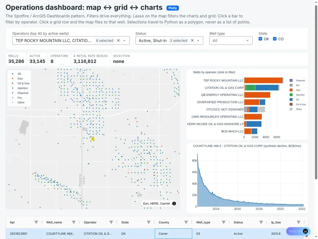
The production decline curves in the app are illustrative rather than from the state databases, and everything else on the page is real data.
Prompt: Build a Dash operations dashboard for the wells with a Plotly well map, a bar chart of wells by operator, a decline curve, KPI tiles and an AG Grid table. Lassoing on the map or the bar chart filters everything else through a clientside callback that sends only the lasso polygon, clicking a bar filters by operator, and clicking a grid row flies the map to that well. Label the decline curves as illustrative.
Drawing, editing and measuring with dash-leaflet
Plotly's shape-drawing tools work on regular charts but not on maps. When users need to sketch an area, edit a boundary or measure a distance, use dash-leaflet. Its EditControl returns drawn shapes to Python as GeoJSON, which can go straight into a spatial query:
Prompt: Add a dash-leaflet map with an EditControl for polygons and rectangles and a MeasureControl in miles and acres. When a shape is drawn, send its GeoJSON to DuckDB and estimate the people inside it from census tract populations, weighted by the share of each tract's area inside the shape.
This will create code like this:
import dash_leaflet as dldl.Map(center=[35.5, -97.5], zoom=10, children=[dl.TileLayer(),dl.FeatureGroup([dl.EditControl(id="draw", draw=dict(polyline=False, marker=False, circle=False))]),dl.MeasureControl(position="topleft", primaryLengthUnit="miles", primaryAreaUnit="acres"),])@callback(Output("results", "children"), Input("draw", "geojson"))def people_in_shape(shapes):poly = shapes["features"][-1]["geometry"]return duck.execute("""WITH shape AS (SELECT ST_GeomFromGeoJSON(?) AS g)SELECT round(sum(people * ST_Area(ST_Intersection(geom, g)) / ST_Area(geom)))FROM tracts, shape WHERE ST_Intersects(geom, g)""", [json.dumps(poly)]).fetchone()[0]
When someone draws a polygon, the callback gets it as GeoJSON and DuckDB estimates how many people live inside it from census tract populations, counting each tract in proportion to how much of its area falls inside the shape. The tract table only needs a population column and a geometry, and the same areal weighting drives the wildfire example in the next section. MeasureControl adds distance and area measurement in miles and acres without any callback at all.
Can a Dash map use your existing ArcGIS services?
Yes, and that matters during a migration, because ArcGIS Server usually keeps running for a while after the first Dash apps ship. A feature service query with f=geojson is a GeoJSON API. A tiled MapServer is an XYZ tile URL (with the row before the column, {z}/{y}/{x}). A dynamic MapServer, which draws images on request, becomes a raster source when you point it at the /export endpoint with bbox={bbox-epsg-3857} in the URL, which MapLibre fills in for each tile. This is the FEMA flood zone layer from the map at the top of this post:
Prompt: Add FEMA's NFHL flood hazard zones (layer 28) to a Plotly map as a raster layer from the MapServer /export endpoint, with bbox={bbox-epsg-3857}, 256-pixel PNG tiles, dpi=10 and the layer drawn below the traces at 75% opacity.
This will create code like this:
source = ["https://hazards.fema.gov/arcgis/rest/services/public/NFHL/MapServer/export""?bbox={bbox-epsg-3857}&bboxSR=3857&imageSR=3857&size=256,256&dpi=10""&format=png32&transparent=true&layers=show:28&f=image"]layers = [dict(sourcetype="raster", source=source, below="traces", opacity=0.75)]
Check each layer's scale range before you wire it up. FEMA's flood hazard zones (layer 28) only draw at 1:36,112 or closer, and ArcGIS works out the scale from the image's dpi, so at the default 96 dpi every 256-pixel tile came back empty until tile zoom 14. With dpi=10 the zones draw from tile zoom 11, which is the whole of Houston on one screen. Dynamic exports are also slow at low zoom, since the server draws every tile from scratch: when we tried a wider view of Houston and Galveston Bay at tile zoom 10, single tiles took up to 34 s and two of 30 timed out, so give layers like this a minzoom.
The Houston map mixes four kinds of service in one Plotly figure: USGS Topo tiles from an ArcGIS tiled MapServer, FEMA's flood zones from a dynamic MapServer's /export, NOAA's radar mosaic over OGC WMS (live, and dry when we rendered it), and USGS stream monitoring sites from the USGS Water Data OGC API as a Plotly trace, with a legend that toggles like an ArcGIS layer list. Here's how the usual ArcGIS pieces map onto Dash:
ArcGIS
In Dash
Map service, tiled or dynamic
Vector tiles from DuckDB or PostGIS, or the existing MapServer as a raster source
Feature service query
A bounding-box query from the map's viewport, or a GeoJSON route
Basemap gallery
layout.map.style built from Esri, USGS and CARTO tile URLs
Layer list and visibility ranges
The Plotly legend for traces, and minzoom and maxzoom on style layers
Symbology and Arcade expressions
MapLibre paint expressions, changed from callbacks with Patch()
Sketch and Measure widgets
dash-leaflet EditControl and MeasureControl
Buffer, Near and Spatial Join tools
DuckDB spatial or PostGIS SQL
Hexbin aggregation
H3 cells precomputed per row and a GROUP BY
ArcGIS Dashboards, Spotfire marking
selectedData, a clientside callback, SQL, then AG Grid and charts
Simple 3D scenes
A fill-extrusion layer plus map pitch
Live ArcGIS data joined in SQL: people living near current wildfires
Analysis works the same way. During fire season, emergency managers and insurers want to know how many people live near each fire, and the perimeters are already public as an ArcGIS feature service. Our example pulls the current interagency fire perimeters that the National Interagency Fire Center (NIFC) publishes through WFIGS, its wildland fire information service (f=geojson&outSR=4326, paged with resultOffset), buffers them by 5 miles in DuckDB, and joins the buffers against 83,508 census tracts in the lower 48 with their population from the Census Bureau's American Community Survey (ACS) for 2019-2023. A tract that is partly inside a buffer counts in proportion to its area inside it, which assumes people are spread evenly within the tract:
Prompt: In DuckDB, buffer each fire perimeter by 5 miles in EPSG:5070 and union the pieces per fire, then join the buffers to census tracts and sum each tract's population weighted by the share of its area inside the buffer, sorted by people within 5 miles.
This will create code like this:
CREATE TABLE fire_buffers ASSELECT fire_id, ST_Union_Agg(ST_Buffer(part, 8046.72)) AS buf -- 5 miles, in EPSG:5070 metersFROM (SELECT fire_id, unnest(ST_Dump(geom)).geom AS part FROM fires)GROUP BY fire_id;SELECT f.name, sum(t.people * ST_Area(ST_Intersection(t.geom, b.buf)) / ST_Area(t.geom)) AS people_withinFROM fire_buffers b JOIN tracts t ON ST_Intersects(t.geom, b.buf) JOIN fires f USING (fire_id)GROUP BY f.name ORDER BY people_within DESC;
On November 4, 2026 the layer held 77 perimeters, 70 of them wildfires and the rest prescribed burns. NIFC keeps recent fires in it as well as ongoing ones, so many were already contained. About 918,279 people lived within 5 miles of one of the 70, and 728,609 of them were near three small fires on the edge of cities: a 0.27-acre fire north of Boston (369,190 people), the 570-acre Norte fire in Orange County (200,717) and the 30-acre Market fire north of Spokane (158,702). The largest fire in the layer, the 278,899-acre Ranger Road fire in Oklahoma, had 4,860. Fetching the perimeters took about 5 s, buffering them about 4 s and the per-fire join 0.1 s. The map below shows the result for all 70 wildfires and zooms in on the three fires near cities.
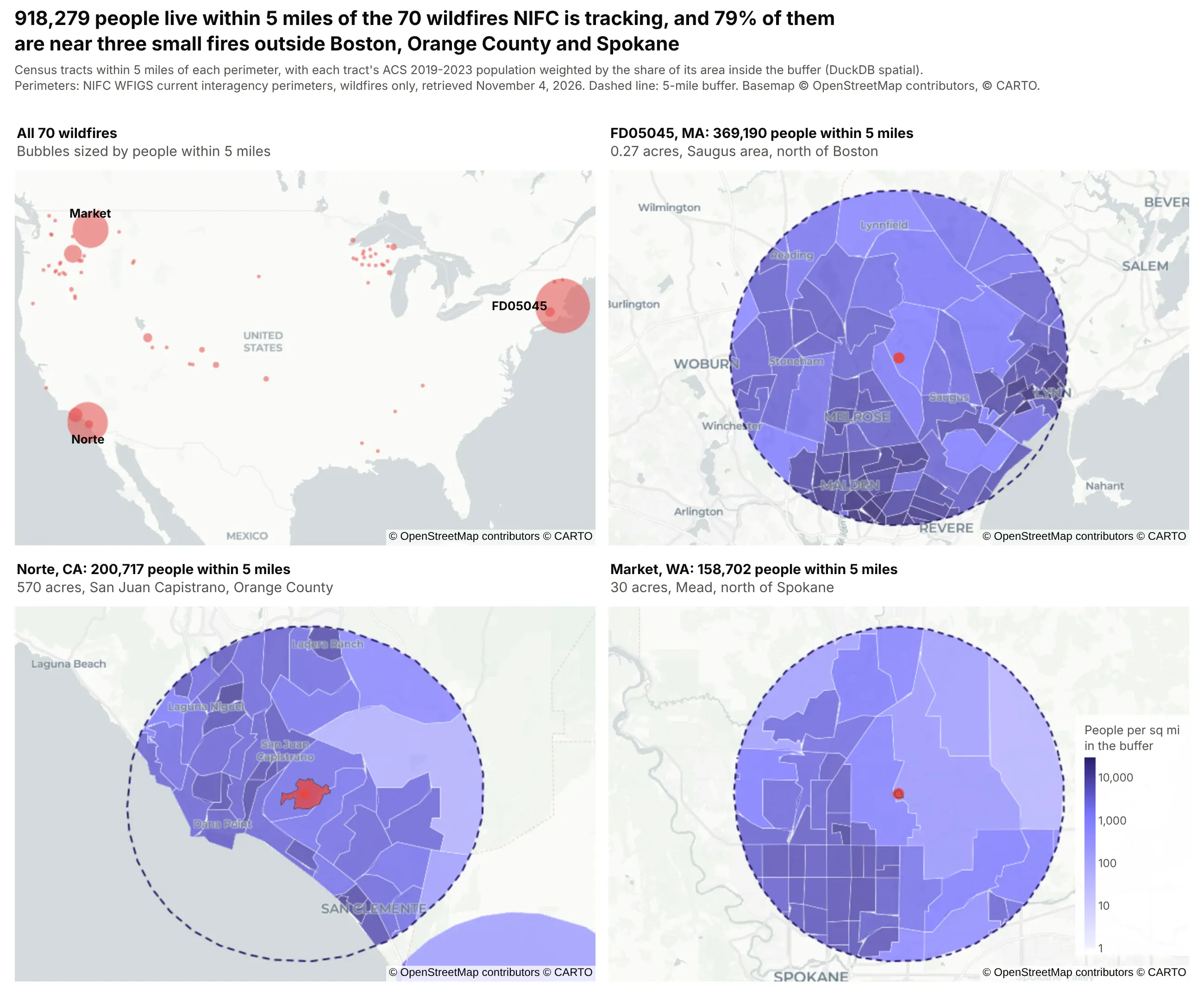
Prompt: Fetch NIFC's WFIGS current interagency fire perimeters from its ArcGIS feature service as GeoJSON, buffer each wildfire by 5 miles in DuckDB in EPSG:5070, and estimate the people within each buffer from census tract ACS population, weighting each tract by its share of area inside. Draw a four-panel Plotly figure: every wildfire as a bubble sized by people nearby, and zoomed maps of the three fires with the most people, each with its dashed buffer and the tract pieces shaded by people per square mile.
These wildfire and flood examples weren't our first choice. While we were staging this set of posts, an automated safety check stopped our coding agent partway through publishing maps that combined energy infrastructure (pipelines, LNG terminals and transmission lines) with hazards like hurricanes and wildfires. All of it was public government data, but we replaced those examples with the population and flood maps above. If your team maps its own assets against hazards, expect AI coding tools to be cautious with that kind of map too.
DuckDB or PostGIS for maps in Dash?
The app runs on DuckDB with the spatial extension by default, and setting DATABASE_URL switches every page to PostGIS, since each query is written in both dialects. DuckDB runs inside the Python process and reads GeoParquet files directly, so there's nothing to operate, which makes it the simpler choice when the data is a few GB and belongs to one app. PostGIS fits better when the data is shared between apps, updated continuously, already lives there, or is bigger than the app server's memory. The SQL carries over almost line for line, and the vector tiles post has tile query timings for both.
Three things about spatial SQL we learned the slow way, re-measured on the wildfire join above (70 fires against 83,508 tracts) in DuckDB 2.0 on a 4-vCPU container:
- Keep the distance in a proximity join a constant. With a literal distance, ST_DWithin(t.geom, f.geom, 8046.72) plans as a spatial join and took 0.09 s, about the same as ST_Intersects against a precomputed buffer (0.05 s). When the distance came from a column instead (as it does if you scale a Web Mercator distance by latitude per row), DuckDB fell back to a nested loop join that tested every pair and took 342 s for the same 439 matches. Projecting to an equal-area CRS such as EPSG:5070 keeps the distance a constant. In PostGIS, ST_DWithin on geography is the idiomatic, index-assisted way.
- Split multipolygons with ST_Dump before buffering them. Fire perimeters arrive as multipolygons with many spot-fire parts (2,256 parts across these 70 fires), and buffering them whole took 21.5 s. Dumping first, buffering each part and unioning the parts per fire took 4.2 s and gave the same total area.
- Use a file-backed DuckDB in small containers. An in-memory database has to keep every table in RAM, while a file-backed one with memory_limit set can page table data to disk. Loading the tables and running the join in a fresh process left it at a median of 274 MB resident with a file-backed database, against 395 MB in memory (three runs each, memory_limit of 300 MB). The peak was closer, about 440 MB file-backed and 500 MB in memory, so size the container for the peak. On DuckDB 1.5.6 the same test came out the other way round, so measure on the version you deploy.
Deploying map apps on Dash Enterprise or Plotly Cloud
A map app deploys like any other Dash app. Dash Enterprise runs it inside your own cloud account or data center, next to your PostGIS database and behind your company's login, which is usually what a replacement for ArcGIS Server or Spotfire Server needs, since operational data rarely leaves the network. Plotly Cloud is the quickest way to share one, and the example app in this post ran in a standard container with 1 GB of memory and half a CPU. A few settings mattered on both:
- Run one gunicorn process with many threads. A map requests 10 to 30 tiles at once, and the default sync worker answers them one at a time. Threads share the data in memory, where extra processes would each hold their own copy. Put workers = 1, worker_class = "gthread" and threads = 8 or more in a gunicorn.conf.py in the app folder.
- Build tile and GeoJSON URLs from the request's Origin header. Both platforms run apps behind an HTTPS proxy, so Flask sees http://, and a tile URL built from request.host_url gets blocked by the browser as mixed content.
- Keep the DuckDB file on the persistent filesystem. Both platforms mount a persistent directory and set DASH_DATA_DIR. Store the database there and the tables and spatial indexes are built once, then reused on every restart and redeploy.
- Build data in a background thread. Loading GeoParquet and building indexes at import time can take long enough that a small container misses its first health check. Start the build in a thread and have the map callbacks wait for it.
- Size DuckDB from the container's memory, so the same code fits a 1 GB instance and uses all of a larger one.
- import flask, not from flask import request. A module-level request proxy makes the worker fail to start with "Working outside of request context".
What's next for Plotly maps
Building these benchmarks gave us a list of concrete improvements for maps in plotly.js, with the source locations and measurements behind each one, and we've started on them:
- A vector tile trace, so Plotly's choropleth and scatter API (colorscales, hover, click, selection and Patch() updates) works over geometry that streams from SQL, without hand-written MapLibre styles or the workaround for clicks on tile features.
- Typed arrays for markers, so 500,000 points stop becoming 500,000 JavaScript objects and very large scatter layers load faster and use less memory.
- Faster hover and recoloring on large layers, through a spatial index for hover (today it's a linear scan that projects every point on every mouse move) and MapLibre feature-state for choropleth colors, so a Patch() of z stops rebuilding the geometry.
- Paint and filter expressions and click and hover events on map.layers, map.layers sources compared by reference instead of turned into strings, and guards against empty polygons.
- Faster built-in clustering, and a fix for cluster bubbles that are invisible with per-point marker colors unless you set cluster.color yourself.
The first few items are small changes, while the vector tile trace and typed arrays close most of the gap to deck.gl and to an ArcGIS map service, while keeping what makes Plotly maps productive in Dash.
Thanks to the community
Dash's mapping options are much richer because of the people who build and maintain the community libraries in this post. Thank you to Emil Eriksen for dash-leaflet, the go-to choice for GIS tools like drawing and measuring in Dash; Scott Lemke for deckgl-dash, which brings deck.gl 9, binary data and drawing tools to Dash; Ravi Sharma for dash-openlayers, with OGC services, projections, editing tools and fast vector tile rendering; Pip Install Python for dash-leaflet2, an early look at Leaflet 2 in Dash; and Xing Han Lu for dash-deck, the first deck.gl component for Dash. Underneath all of it are MapLibre, Leaflet, deck.gl, OpenLayers, DuckDB and its spatial extension, PostGIS, GEOS, GeoPandas, H3 and tippecanoe.
Summary
Large maps in Dash are mostly a question of how much geometry reaches the browser and how often. Plotly's map traces are the most productive choice up to about 100,000 points or a few thousand polygons, as long as GeoJSON loads by URL and callbacks return Patch() updates. Past that, vector tiles from DuckDB or PostGIS keep a Plotly map at about 2 s however big the table gets, deck.gl through deckgl-dash with binary arrays keeps every point in the browser when that's what users need, and dash-leaflet covers drawing and measuring. Your ArcGIS and WMS services keep working inside the same map while you move. For the rest of the mapping story, from choosing a library to 13 real-data examples, see the Python maps guide.