
Chris Parmer
November 5, 2026
Python Geospatial Libraries Compared: GeoPandas, DuckDB, Polars and SedonaDB (2026)
TL;DR
- We timed four Python libraries on the same eight geospatial jobs (reprojecting, measuring, joining points to polygons, finding the nearest river, buffering and dissolving, clipping, counting by hexagon and writing files), using public US data: 87,028 USGS subwatersheds, 712,768 river reaches and up to 10 million places from Overture Maps. The libraries were GeoPandas 1.2, DuckDB 2.0 with its spatial extension, Polars 2.1 with the polars-st plugin, and SedonaDB 0.5.
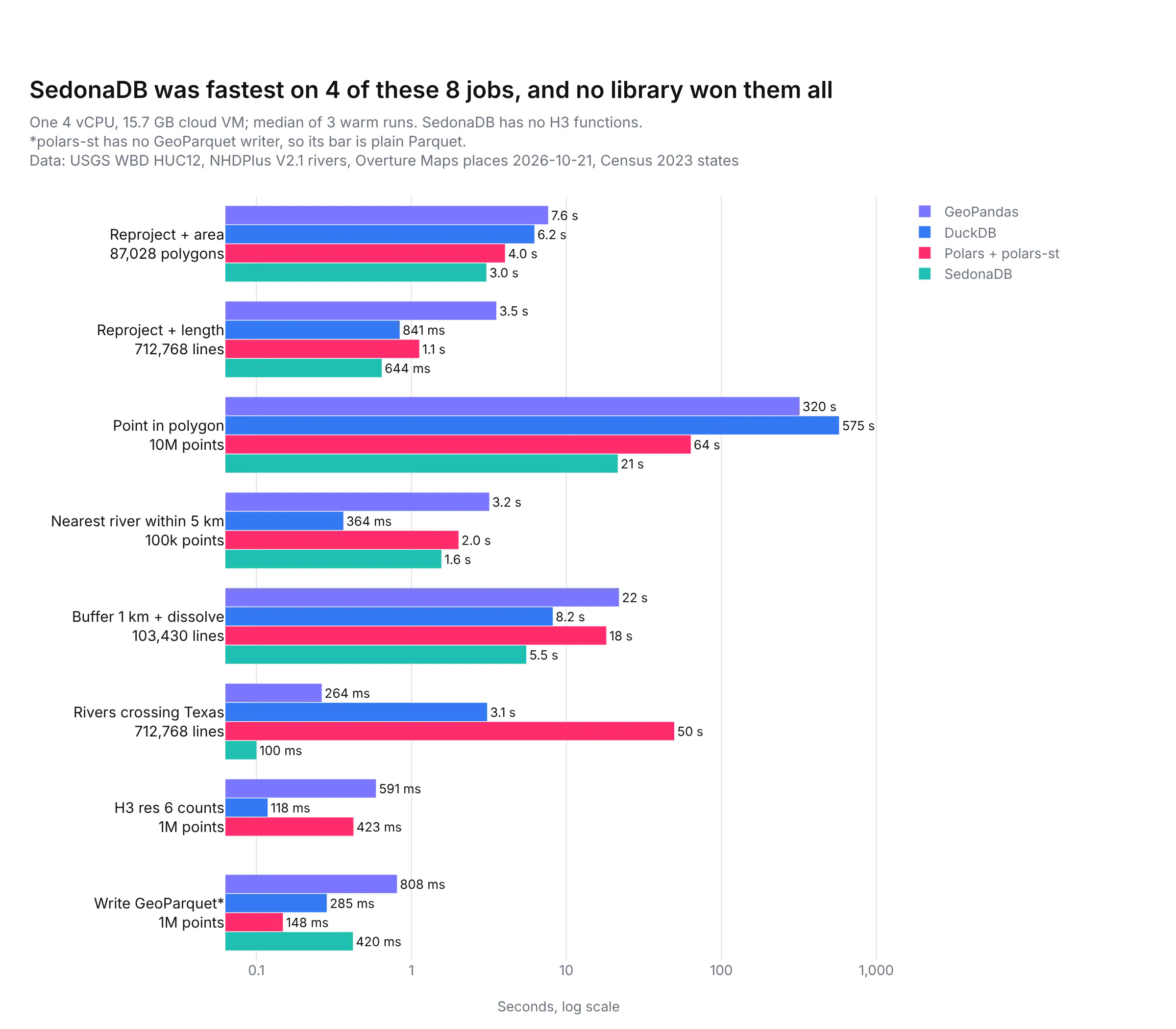
- No library was fastest at everything. As we first wrote the jobs, SedonaDB was fastest on 4 of the 8, including counting 10 million points per watershed in 21.5 s with no extra preparation, and DuckDB was fastest at finding the nearest river (0.36 s for 100,000 points) and counting points per hexagon (0.12 s for 1 million).
- How you write the query mattered more than which library you picked. In our tests, writing the same job differently made it 14 to 105 times faster in all four libraries. GeoPandas went from 320 s to 23.3 s on the 10 million point join just by joining from the polygons instead of the points, and DuckDB went from 575 s to 8.0 s once the watershed outlines were split into small pieces (which took 133 s, once).
- Our recommendation: keep GeoPandas as the default for analysis that fits in memory and needs the widest set of tools, use DuckDB when the data lives in Parquet files or a database and the work is SQL-shaped, and try SedonaDB for heavy joins while remembering it's a young 0.x project. polars-st works for Polars users today, and GeoPolars is still a prototype.
This post compares the Python geospatial libraries on real data, with these results for the eight jobs we timed:
A lot of the teams we work with in energy, finance and pharma are moving their geospatial work off ArcGIS and onto Python, because the rest of their analysis already lives there and they want the maps and the models in one place. The first library they find is GeoPandas, which puts a geometry column on a pandas DataFrame and covers almost everything an ArcGIS user does in a geoprocessing tool. In our DuckDB vs Polars vs pandas benchmark, though, we recommended DuckDB and Polars over pandas for anything big, because they use every CPU core and read Parquet files much faster. That raises the question this post answers: is there a DuckDB or Polars for geospatial work, and is it worth switching?
There are now several real options. DuckDB's spatial extension runs geospatial SQL, Polars has a community plugin called polars-st, and SedonaDB is a new single-machine engine from the Apache Sedona project. We describe each one, then time all four (plus dask-geopandas, which runs GeoPandas in parallel) on the same jobs and the same data, check that they return the same answers, and finish with which one to use when. Every benchmark is in the post's code/ folder, and every code block comes with a prompt you can give a coding agent such as Claude Code or Codex to rebuild it. This post is part of our Python maps guide, which covers drawing the results on a map.
What are the Python geospatial libraries in 2026?
Geospatial analysis in Python means working with tables where one column holds shapes: points (a store, a well, a weather station), lines (a river, a road) or polygons (a county, a watershed, a sales territory). The common jobs are reprojecting (converting coordinates from one coordinate reference system, or CRS, to another, for example from longitude and latitude to meters), measuring areas and lengths, spatial joins (which polygon is each point in?), nearest-neighbour searches, buffers and dissolves, and clipping to a boundary.
Under almost all of these libraries sits GEOS, the C++ geometry engine that also powers PostGIS and QGIS, and most of them store shapes as WKB (well-known binary, a standard compact byte format for geometry). They differ in how they run the work: one row at a time in Python objects, in SQL across every core, or as Polars expressions.
Library
What it is
Latest version (date)
License
pandas DataFrame with a column of Shapely (GEOS) geometries
1.2.0 (2026-09-28)
BSD-3-Clause
SQL engine with a GEOMETRY type in core and spatial functions in the spatial extension
DuckDB 2.0.0 (2026-10-21)
MIT
GEOS-based geometry expressions for Polars, from an independent developer
0.11.0 (2026-10-19), on Polars 2.1.0
LGPL-2.1
Rust engine for one machine, built on Apache Arrow and Apache DataFusion, from the Apache Sedona project
0.5.0 (2026-10-08)
Apache-2.0
GeoPandas split into partitions and run in parallel by Dask
0.5.0 (2025-06-02)
BSD-3-Clause
The Polars project's planned geospatial extension
0.1.0a4 (2022-11-14), a prototype
MIT
GeoPandas
GeoPandas is the standard, and the one every other library is measured against. Its geometry column holds Shapely objects, so every GEOS operation is one vectorized call, and its sjoin, sjoin_nearest, dissolve, clip, overlay and to_crs methods map almost one to one onto the ArcGIS geoprocessing tools. It reads shapefiles, file geodatabases, GeoPackages and GeoJSON through pyogrio and GDAL (the open source library behind most GIS file formats), and GeoPandas 1.2 reads and writes GeoParquet 2.0. Its gaps are scale and speed: it runs on one CPU core, and each geometry is a Python object, which used the most memory of any library in our tests. Use it as the default whenever the data fits comfortably in memory, and whenever you need a method nobody else has yet.
DuckDB spatial
DuckDB is an in-process SQL database, which means it runs inside your Python process with nothing to install or run alongside it, and it's one of the two engines we recommended in our earlier DuckDB vs Polars vs pandas tests. Since DuckDB 1.5 in March 2026, GEOMETRY is a core data type with the coordinate system stored in the column type, so a query that mixes coordinate systems fails instead of returning a quietly wrong answer. The spatial extension adds over 150 functions (ST_Transform, ST_Intersects, ST_Buffer, ST_AsMVT for vector tiles and many more), reads any GDAL vector format with ST_Read, and plans spatial joins with a SPATIAL_JOIN operator that builds an R-tree (a spatial index of bounding boxes) on the fly. The community h3 extension adds H3, Uber's grid of hexagons covering the globe, which is a common way to count points by area. DuckDB 2.0 is a long-term support release with support until at least October 2027, and it makes one change everyone upgrading from 1.x will hit: ST_Transform on longitude and latitude data now raises an error unless you run SET geometry_always_xy = true first. Use DuckDB when the data already sits in Parquet files or a database and the work reads naturally as SQL.
Polars with polars-st, and GeoPolars
Polars has no geometry type of its own yet. The practical option today is polars-st, a plugin written by one developer, Aurèle Ferotin, which is not affiliated with the Polars project. It stores geometries as WKB in ordinary binary columns and adds about 115 GEOS-based expressions under .st, plus a spatial join and to_geopandas(). Because it links GEOS statically, it's licensed under the LGPL, which asks anyone who distributes a changed version of the library to share those changes. It's at version 0.11 and had 6 releases between September 14 and October 19, 2026, so expect the API to move.
GeoPolars is the Polars project's own planned extension, built on GeoArrow (the Apache Arrow standard for geometry columns). Its README still calls it a prototype that "should not be considered production-ready", and its only PyPI release is 0.1.0a4 from November 2022, which was still true when we checked PyPI on November 5, 2026. A rewrite on native GeoArrow types is on its development branch, and on November 2 a maintainer wrote that they hoped to publish an alpha the following week. Polars 2.1 also added experimental GeoParquet reading and writing behind environment variables, which we covered in our Polars 2.1 post.
SedonaDB
SedonaDB is a single-machine analytical database for geospatial data from the Apache Sedona project, written in Rust on Apache Arrow and Apache DataFusion (a Rust SQL query engine) and first released in September 2025. You run SQL on it from Python, it reads GeoParquet natively and other formats through pyogrio, it tracks the coordinate system of every column and raises an error when a query mixes them, and it has a KNN join (k nearest neighbours: for every row on one side, the k closest rows on the other) that GeoPandas and DuckDB don't have built in. It was the fastest library on half of our jobs. It's also young: version 0.5.0, a GeoPandas-style API its authors call "still experimental", no H3 functions yet, and a release post that says "we're still not quite ready to make a splash". The best-known published benchmark of it, SpatialBench, was designed and run by the Apache Sedona project itself, which is why we ran our own.
dask-geopandas, Sedona on Spark and GPUs
dask-geopandas splits a GeoDataFrame into partitions and runs GeoPandas on each in parallel, which gave a near drop-in speedup on the jobs we ran it on, although it hasn't had a release since June 2025. When the data no longer fits on one machine, Apache Sedona on Spark (1.9.1, with a GeoPandas-compatible API since 1.8) is the established option. On GPUs, NVIDIA paused development of cuSpatial in 2025 and stopped publishing new packages, so there is no maintained RAPIDS option for vector geospatial work in Python.
How did we benchmark the libraries?
We picked three public US datasets that look like the layers our customers join every day, and that are big enough for the libraries to separate:
- Watersheds: all 87,028 HUC12 subwatersheds in the lower 48 states, from the USGS Watershed Boundary Dataset. A HUC12 (hydrologic unit code, 12 digits) is the smallest drainage area in that dataset, and the polygons are detailed, with 461 vertices each on average. They stand in for any detailed polygon layer: counties, sales territories, insurance rating zones or flood zones.
- Rivers: 712,768 river reaches of stream order 3 and up (leaving out the smallest headwater streams) from NHDPlus, the national stream network the EPA and USGS maintain. They stand in for any large line layer, such as roads or routes.
- Places: 18,321,320 points of interest in the lower 48 from the Overture Maps Foundation places dataset (release 2026-10-21), sampled down to 100,000, 1 million and 10 million points. These stand in for customer addresses, transactions or sites.
- Texas: the state boundary from the Census Bureau, for the clip test.
Every job ran in a fresh Python process on one cloud machine with 4 virtual CPUs (Intel Xeon at 2.1 GHz) and 15.7 GB of memory. The data was loaded into each library's own in-memory form first and not timed, except in the file reading tests, and then each job ran once to warm up and three more times, and we report the median. Jobs whose warm-up took over 90 seconds got one timed run instead of three, and anything over 600 seconds was stopped. DuckDB, Polars and SedonaDB used all 4 cores, and GeoPandas used one, because that's how each runs out of the box. Areas, lengths, buffers and distances were computed in meters in the US Albers equal-area projection (EPSG:5070).
Prompt: Write a Python benchmark that times GeoPandas, DuckDB spatial, Polars with polars-st and SedonaDB on the same geospatial jobs: reproject and measure, point in polygon counts, nearest feature within 5 km, buffer and dissolve, clip, H3 counts, read and write GeoParquet. Load each input once per process into the library's own format, run each job in a fresh subprocess with one warm-up and the median of three runs, record peak memory, and write the results to a CSV.
The full benchmark is in the post's code/ folder, with a SOURCES.md that lists every number, version and data source.
Which Python geospatial library was fastest?
The chart at the top of this post has the eight jobs side by side. In summary:
- SedonaDB was fastest at 4 of them: reprojecting and measuring the river lengths (0.64 s), counting 10 million points per watershed (21.5 s), buffering and dissolving the large rivers (5.5 s) and selecting the rivers that cross Texas (0.10 s). It was also fastest to reproject and measure the watershed areas among the four main libraries (3.0 s), although dask-geopandas edged it at 2.6 s.
- DuckDB was fastest at finding the nearest river reach for 100,000 points (0.36 s) and counting 1 million points per H3 hexagon (0.12 s), and it used the least memory on the big join. It was the slowest at the point in polygon join as first written, and the fastest once the polygons were split into pieces, which the next section explains.
- Polars with polars-st was fastest to write 1 million points (0.15 s), but only because it has no GeoParquet writer yet, so its file is plain Parquet without the GeoParquet metadata. It was the slowest at selecting the rivers that cross Texas, 50 s against 0.26 s in GeoPandas, because a plain filter with .st.intersects() tests every river against the full outline of Texas without a spatial index.
- GeoPandas was never the fastest of the four, but it was second at selecting the rivers that cross Texas (0.26 s) and reached 23.3 s on the 10 million point join once the join was written from the polygon side.
Point in polygon: how fast can you count 10 million points per watershed?
Counting points per polygon is the spatial join most people run first, whether it's customers per sales territory, claims per flood zone or trial sites per county. Here we counted Overture places in each of the 87,028 watersheds at three sizes:
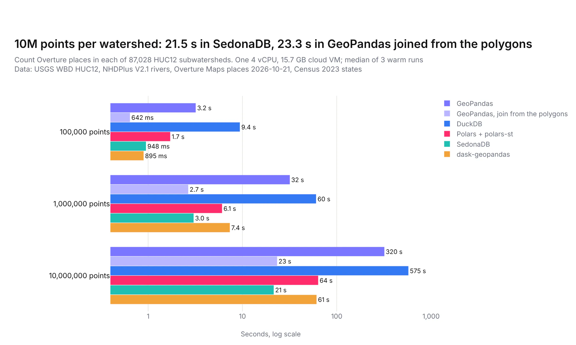
SedonaDB and GeoPandas joined from the polygons were close at every size, about 21 to 23 s for 10 million points, with no extra preparation. dask-geopandas and polars-st took about 1 minute, and the plain GeoPandas join took 320 s.
DuckDB was the slowest at this join as we first wrote it, 575 s for 10 million points, and that surprised us, because DuckDB's own spatial join post joined 58 million bike trips to 310 New York neighborhoods in 28.7 s on a laptop. We checked the query plan with EXPLAIN, and it did use DuckDB's SPATIAL_JOIN operator, so the index was working. Switching the test from ST_Intersects to ST_Contains only brought it to 436 s.
The difference turned out to be the polygons. New York neighborhoods are simple shapes, while our watersheds average 461 vertices each. Our best explanation, which we didn't measure directly, is that DuckDB tests each candidate point against the full outline without the prepared geometry GEOS uses to speed that up. So we split every watershed into pieces of at most 64 vertices with ST_Subdivide, which turned 87,028 outlines into 1,153,213 pieces. On the pieces, the 1 million point join took 0.96 s instead of 44 s in the same test run (the benchmark's median for the full outlines was 60 s), and the 10 million point join took 8.0 s instead of 575 s, faster than any other library in this test. Splitting the outlines took 133 s, but you only do it once and can save the pieces to a file.
The counts matched with one small catch. At 1 million points, the split version agreed with the original join except for the 2 points that sit on a boundary between two watersheds. At 10 million points, 27 points (each in a different watershed) were missing compared with GeoPandas, most likely because ST_Contains doesn't count a point that falls exactly on one of the new cut lines (we didn't check them one by one). Joining the pieces with ST_Intersects and counting distinct points per watershed should avoid that, but we didn't time that version.
Prompt: In DuckDB with the spatial extension, split each HUC12 watershed polygon into pieces of at most 64 vertices with ST_Subdivide and ST_Dump, save them to a table, then count points per huc12 by joining the points to the pieces with ST_Contains.
This will create code like this:
import duckdbcon = duckdb.connect()con.sql("LOAD spatial; SET geometry_always_xy = true")con.sql("CREATE TABLE w AS SELECT huc12, geometry FROM read_parquet('watersheds.parquet')")con.sql("CREATE TABLE p AS SELECT geometry FROM read_parquet('points_10m.parquet')")# once: 133 s, 87,028 outlines -> 1,153,213 pieces of at most 64 verticescon.sql("""CREATE TABLE w_sub ASSELECT huc12, unnest(ST_Dump(ST_Subdivide(geometry, 64))).geom AS geometry FROM w""")# 8.0 s for 10M points, against 575 s on the full outlinescounts = con.sql("""SELECT w.huc12, count(*) AS nFROM p JOIN w_sub w ON ST_Contains(w.geometry, p.geometry)GROUP BY w.huc12""").df()
The same idea should help in any engine that tests points against detailed polygons, since each test does less work on a small piece, although we only measured it in DuckDB.
Why does how you write the query matter more than which library you use?
The biggest differences in the whole benchmark came from writing the same job differently, not from switching libraries. In each pair below, both versions return the same result, which we checked row by row (apart from the 27 points on cut lines in DuckDB's split version, described above):
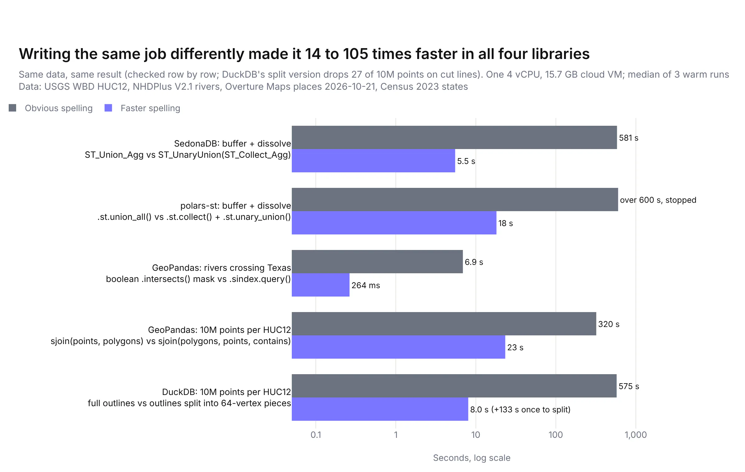
There's a pattern behind all of them. A spatial engine is fast when it can prepare a shape once and reuse it, or skip most shapes with an index, and the obvious spelling often stops it from doing either.
Join from the polygons in GeoPandas. gpd.sjoin(points, polygons) and gpd.sjoin(polygons, points, predicate="contains") give the same pairs. When the polygons are on the left, GEOS prepares each watershed outline once (precomputing an index of its edges) and tests every candidate point against the prepared version, which took the 10 million point join from 320 s to 23.3 s and the 1 million point join from 31.8 s to 2.7 s.
Prompt: Count how many points fall in each polygon with GeoPandas. Use gpd.sjoin with the polygons as the left frame and predicate="contains", so GEOS prepares each polygon once, then group by the polygon id and count.
This will create code like this:
import geopandas as gpd# slow: 320 s for 10M pointsjoined = gpd.sjoin(points, watersheds[["huc12", "geometry"]], predicate="intersects")# fast: 23.3 s, same countsjoined = gpd.sjoin(watersheds[["huc12", "geometry"]], points, predicate="contains")counts = joined.groupby("huc12").size().rename("n").reset_index()
Use the spatial index to clip in GeoPandas. A boolean mask, rivers[rivers.intersects(texas)], tests all 712,768 reaches against the full Texas outline. rivers.sindex.query(texas, predicate="intersects") first uses the R-tree to throw away every reach whose bounding box misses Texas, and only tests the rest, which took the clip from 6.9 s to 0.26 s. GeoPandas's own gpd.clip uses the index too, but it also cuts the lines at the border, which is a different job.
Prompt: Select the rivers that cross the Texas boundary in GeoPandas using the spatial index: rivers.sindex.query(texas_geometry, predicate="intersects"), then rivers.iloc on the result.
This will create code like this:
texas_geom = texas.geometry.iloc[0]# slow: 6.9 sin_texas = rivers[rivers.intersects(texas_geom)]# fast: 0.26 s, same 26,073 reachesin_texas = rivers.iloc[rivers.sindex.query(texas_geom, predicate="intersects")]
Collect, then union once, in SedonaDB and polars-st. Dissolving buffered rivers by region with ST_Union_Agg in SedonaDB, or .st.union_all() in polars-st, appears to merge the shapes a few at a time, so each region's growing outline gets rebuilt over and over (that's our reading of the timings, not something we profiled). Collecting each region's shapes into one multi-polygon and running a single unary union lets GEOS merge them all in one pass. In SedonaDB that took the job from 581 s to 5.5 s, and in polars-st from over 600 s (we stopped it) to 18 s.
Prompt: In SedonaDB, buffer every river reach of stream order 6 and up by 1,000 m and dissolve the buffers by huc2. Use ST_UnaryUnion(ST_Collect_Agg(ST_Buffer(geometry, 1000))) grouped by huc2 instead of ST_Union_Agg. Then do the same in Polars with polars-st, using .st.collect() in the group_by aggregation and .st.unary_union() afterwards.
This will create code like this:
import sedonadbimport polars as plimport polars_st as stsd = sedonadb.connect()# slow: 581 s with ST_Union_Agg(ST_Buffer(geometry, 1000))# fast: 5.5 sdissolved = sd.sql("""SELECT huc2, ST_UnaryUnion(ST_Collect_Agg(ST_Buffer(geometry, 1000))) AS geometryFROM rivers WHERE stream_order >= 6GROUP BY huc2""").to_pandas()# polars-st: .agg(st.geom().st.buffer(1000).st.union_all()) was stopped after 600 sbig = rivers.filter(pl.col("stream_order") >= 6)merged = big.group_by("huc2").agg(st.geom().st.buffer(1000).st.collect())dissolved = merged.with_columns(st.geom().st.unary_union()) # 18 s
The DuckDB fix, splitting the polygons, is in the point in polygon section above. The lesson for anyone porting a workflow from ArcGIS is to time the obvious version on a sample before running it on everything, because the gap between a working query and a fast one was bigger than the gap between libraries.
Which file format is fastest to read: Shapefile, GeoPackage, FlatGeobuf or GeoParquet?
Most GIS data still arrives as shapefiles or file geodatabases, so we also timed reading the same 87,028 watersheds from four formats. GeoParquet is Parquet with geometry metadata, GeoPackage is a SQLite database file, and FlatGeobuf is a streaming binary format with a built-in spatial index.
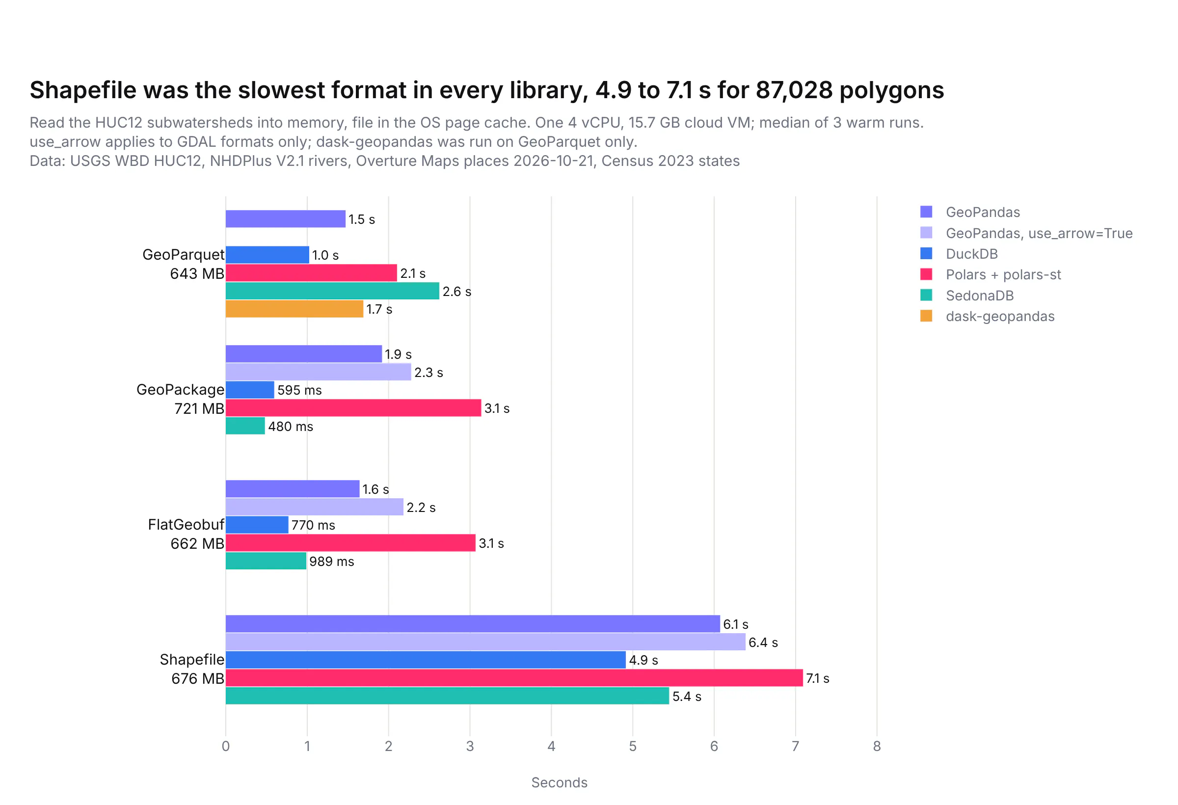
Shapefile was the slowest format in every library, at 4.9 to 7.1 s, while DuckDB and SedonaDB read the GeoPackage in 0.6 s and 0.48 s. Two caveats apply. These reads were from the operating system's cache, so they measure parsing rather than disk speed, and GeoPandas does more work while reading than the others, because it builds a GEOS object for every shape up front where DuckDB, Polars and SedonaDB keep the compact binary form and parse it later. Shapefiles also have hard limits (2 GB per file, 10-character column names), so converting them once to GeoParquet or GeoPackage pays off quickly.
Prompt: Convert a shapefile to GeoParquet with GeoPandas: read it with gpd.read_file and engine pyogrio with use_arrow=True, then write it with to_parquet, and do the same in DuckDB with ST_Read and COPY TO a .parquet file.
This will create code like this:
import duckdbimport geopandas as gpdgdf = gpd.read_file("watersheds.shp", use_arrow=True)gdf.to_parquet("watersheds.parquet")con = duckdb.connect()con.sql("LOAD spatial")con.sql("COPY (SELECT * FROM ST_Read('watersheds.shp')) TO 'watersheds.parquet' (FORMAT parquet)")
How much memory does each library use?
Memory decides whether a job runs on a laptop at all, so we recorded the peak memory of each process, which includes the loaded inputs:
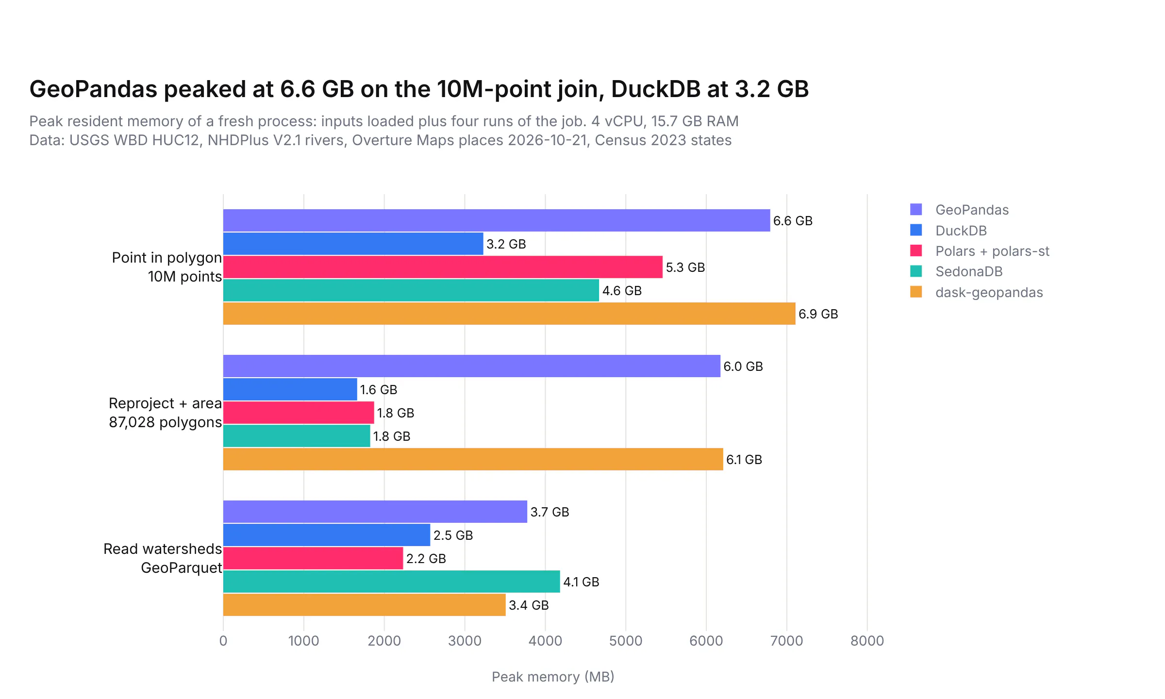
GeoPandas and dask-geopandas used the most, 6.6 GB and 6.9 GB on the 10 million point join and about 6 GB to reproject the watersheds, because every shape is a separate Python object. DuckDB used the least on the big join (3.2 GB) and on the reprojection (1.6 GB).
Did every library get the same answer?
A fast wrong answer is worse than a slow right one, so we compared every library's output with GeoPandas row by row:
- Point in polygon: identical counts per watershed in every library at every size (16,326 watersheds with at least one point at 100,000 points, 38,420 at 1 million and 63,430 at 10 million).
- Areas and lengths: the same as GeoPandas to within a relative difference of 6 in 100 billion for areas and 1.4 in 100 million for lengths, which is floating-point rounding.
- Nearest river: the same 80,016 of the 100,000 points matched a reach within 5 km in every library, at the same distance. For about 2% of points, libraries picked a different reach at exactly the same distance, which happens where two reaches meet.
- Buffer and dissolve: total areas within 0.14% of each other, because each library draws the rounded ends of a buffer with its own number of segments.
- Clip: the same 26,073 reaches in every library.
- H3: DuckDB matched the reference H3 C library for all 1 million points. The packages we used for GeoPandas (h3ronpy) and Polars (polars-h3) put 3 and 2 points in a neighbouring hexagon, because both are built on h3o, a Rust port of H3.
Which Python geospatial library should you use?
If you...
Use
Why
Are starting out, or porting ArcGIS geoprocessing
GeoPandas
The widest set of operations and file formats, the most documentation, and the tool every other library converts to
Have data in Parquet files or a database, and think in SQL
DuckDB spatial
No server, low memory, fast nearest-feature and H3 queries, and long-term support on 2.0
Run heavy spatial joins and aggregations on one machine
SedonaDB
Fastest on half our jobs, with KNN joins built in; test it on your own data, since it's at 0.5
Already use Polars
Polars with polars-st
Spatial expressions inside your Polars pipelines; watch for LGPL, a single maintainer and missing GeoParquet writes
Have data bigger than one machine
Apache Sedona on Spark
Distributed spatial SQL and a GeoPandas-compatible API
Want GeoPandas code to use every core
dask-geopandas
Near drop-in for reads, reprojection and joins, though it hasn't had a release since June 2025
The libraries also work well together. DuckDB and SedonaDB can read a GeoDataFrame and hand results back to GeoPandas, and polars-st has to_geopandas(), so a common setup is to do the heavy filtering and joining in DuckDB or SedonaDB, then finish in GeoPandas and draw the result with Plotly.
Prompt: Count Overture places per HUC12 watershed in SedonaDB, convert the result to a GeoDataFrame with the watershed outlines, and draw it with plotly.express choropleth_map, colored by places per square kilometer, on the carto-positron basemap.
This will create code like this:
import plotly.express as pximport sedonadbsd = sedonadb.connect()sd.read_parquet("watersheds.parquet").to_memtable().to_view("w")sd.read_parquet("places.parquet").to_memtable().to_view("p")counts = sd.sql("""SELECT w.huc12, count(*) AS placesFROM p JOIN w ON ST_Intersects(w.geometry, p.geometry)GROUP BY w.huc12""").to_pandas()gdf = watersheds.merge(counts, on="huc12") # watersheds is a GeoDataFramegdf["per_km2"] = gdf["places"] / gdf.to_crs(5070).area * 1e6fig = px.choropleth_map(gdf, geojson=gdf.geometry, locations=gdf.index, color="per_km2",map_style="carto-positron", zoom=3, center={"lat": 39, "lon": -96})fig.show()
Summary
There's no single DuckDB-for-geospatial yet. GeoPandas is still the right default, DuckDB spatial is the best fit when your data lives in Parquet or SQL, and SedonaDB was the fastest engine on our heaviest jobs while still being early. The bigger lesson from our tests is that the way you write a job matters more than the library, so join from the polygons in GeoPandas, split detailed polygons before joining in DuckDB, use the spatial index for filters, and collect before you union, then time a sample before you run the whole dataset.