Chris Parmer

October 24, 2026

Lollipop Charts - A Complete Guide

TL;DR

A lollipop chart is a bar chart with each bar drawn as a thin stem and a dot at the value, so it shows the same lengths from zero with much less ink.
Lollipop charts are also known as lollipop plots and stem plots, and are similar to bar charts, dot plots and dumbbell charts.
Use one instead of bars when there are many bars of similar length, values around a benchmark, ordered categories such as months, or events in time.
Stems must start at zero or at a benchmark you name. For a zoomed axis, use a dot plot instead.
You can make a lollipop chart with Plotly from two go.Scatter traces, one for the stems with None between rows and one for the heads, and any coding agent can build one in a minute.

What is a lollipop chart?

Lollipop charts look like this:

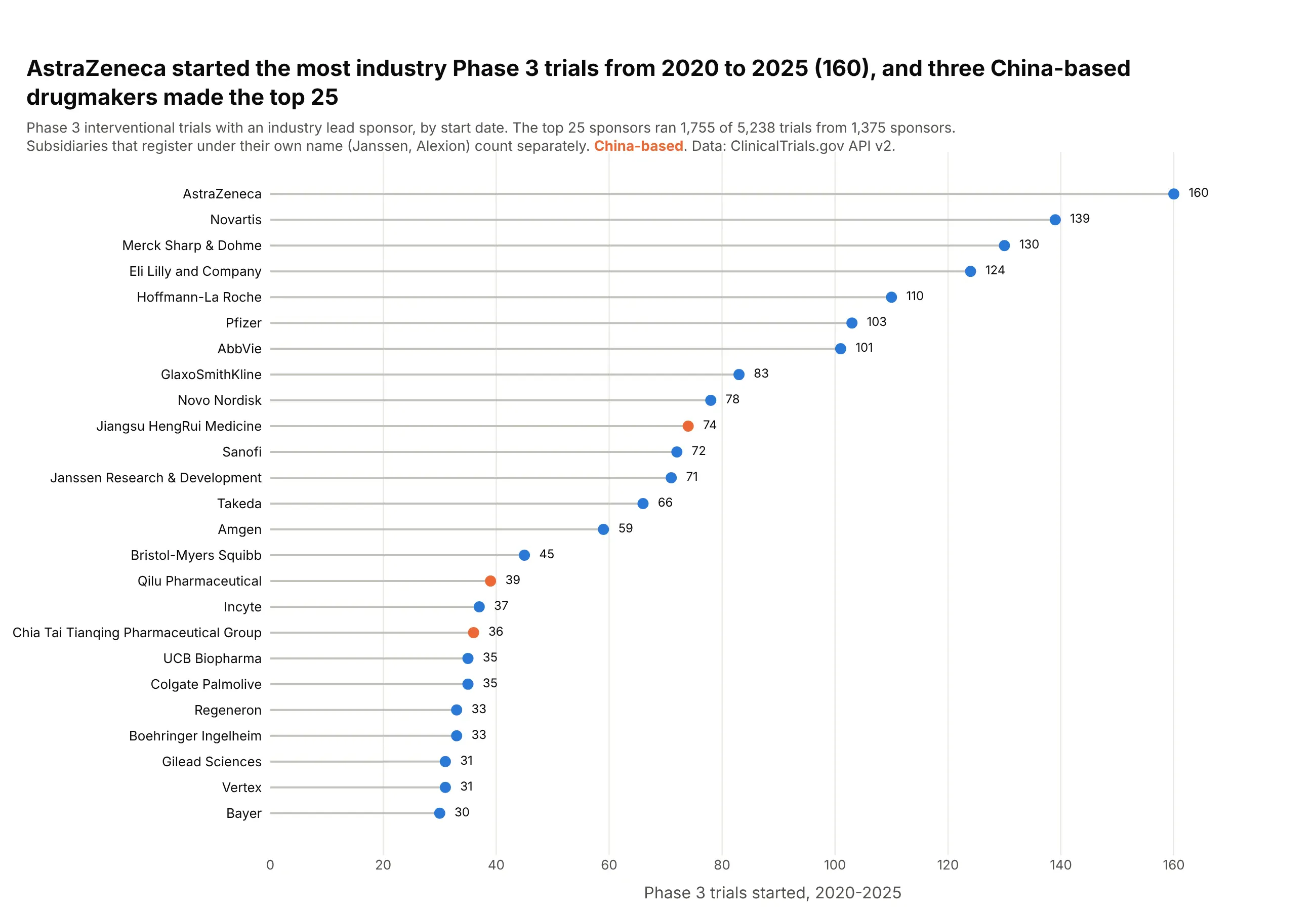
Lollipop chart of the 25 industry sponsors with the most Phase 3 trials started from 2020 to 2025, from AstraZeneca with 160 and Novartis with 139 to Bayer with 30, with Jiangsu HengRui (74), Qilu (39) and Chia Tai Tianqing (36) in orange as China-based

Data: ClinicalTrials.gov API v2, industry-sponsored Phase 3 trials started 2020-2025.

How do you read a lollipop chart? In the example above, notice these things:

Each row is one drug company, and its lollipop is a thin stem from zero to the number of industry Phase 3 trials it started, with a dot at the end.
The stem's length is the value, as with a bar, and every stem starts at zero. That is why AstraZeneca's stem can be read as just over twice as long as Janssen's.
The rows are sorted from the most trials to the fewest, which puts AstraZeneca at the top and shows how gradually the counts fall from Novartis down to Bayer.
The thin stems leave room to print each count next to its dot, and color carries one more fact, so the three China-based sponsors, led by Jiangsu HengRui, stand out in orange.
Sponsors are counted under the name they register with, so a subsidiary like Janssen gets its own row apart from its parent company. Check how the categories were defined before you compare two rows.

It's often used for charts like these:

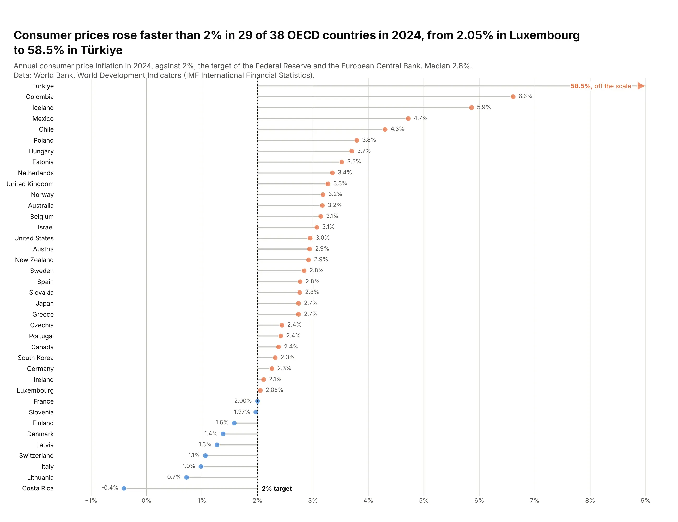
Diverging lollipop chart of 2024 consumer price inflation in the 38 OECD countries with stems growing from a 2% line: 29 above in orange, from 2.05% in Luxembourg to 6.6% in Colombia, Türkiye's 58.5% drawn as an arrow off the scale, and 9 at or below in blue down to -0.4% in Costa Rica

Distance from a target. With stems that grow from 2% instead of zero, consumer prices rose faster than that in 29 of the 38 OECD countries in 2024, and Türkiye's 58.5% is drawn as an arrow off the scale. Data: World Bank, World Development Indicators (IMF).

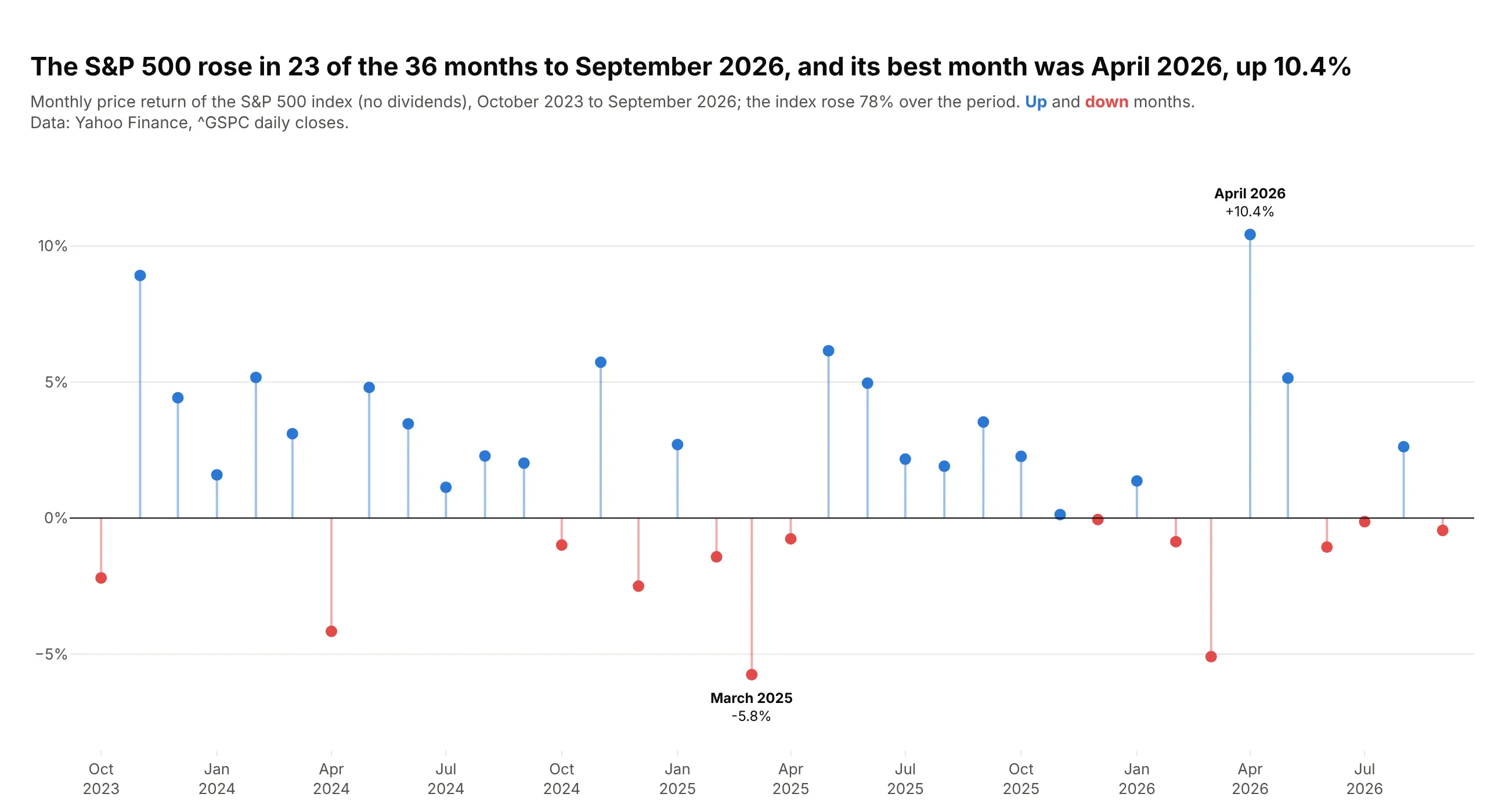
Vertical lollipop chart of the S&P 500's monthly price return from October 2023 to September 2026, blue stems up and red stems down from zero, with the best month, April 2026 (+10.4%), and the worst, March 2025 (-5.8%), labeled

Gains and losses over time. The S&P 500 rose in 23 of the 36 months to September 2026, and the stems show the size of each month around zero, from -5.8% in March 2025 to +10.4% in April 2026. Data: Yahoo Finance, ^GSPC daily closes.

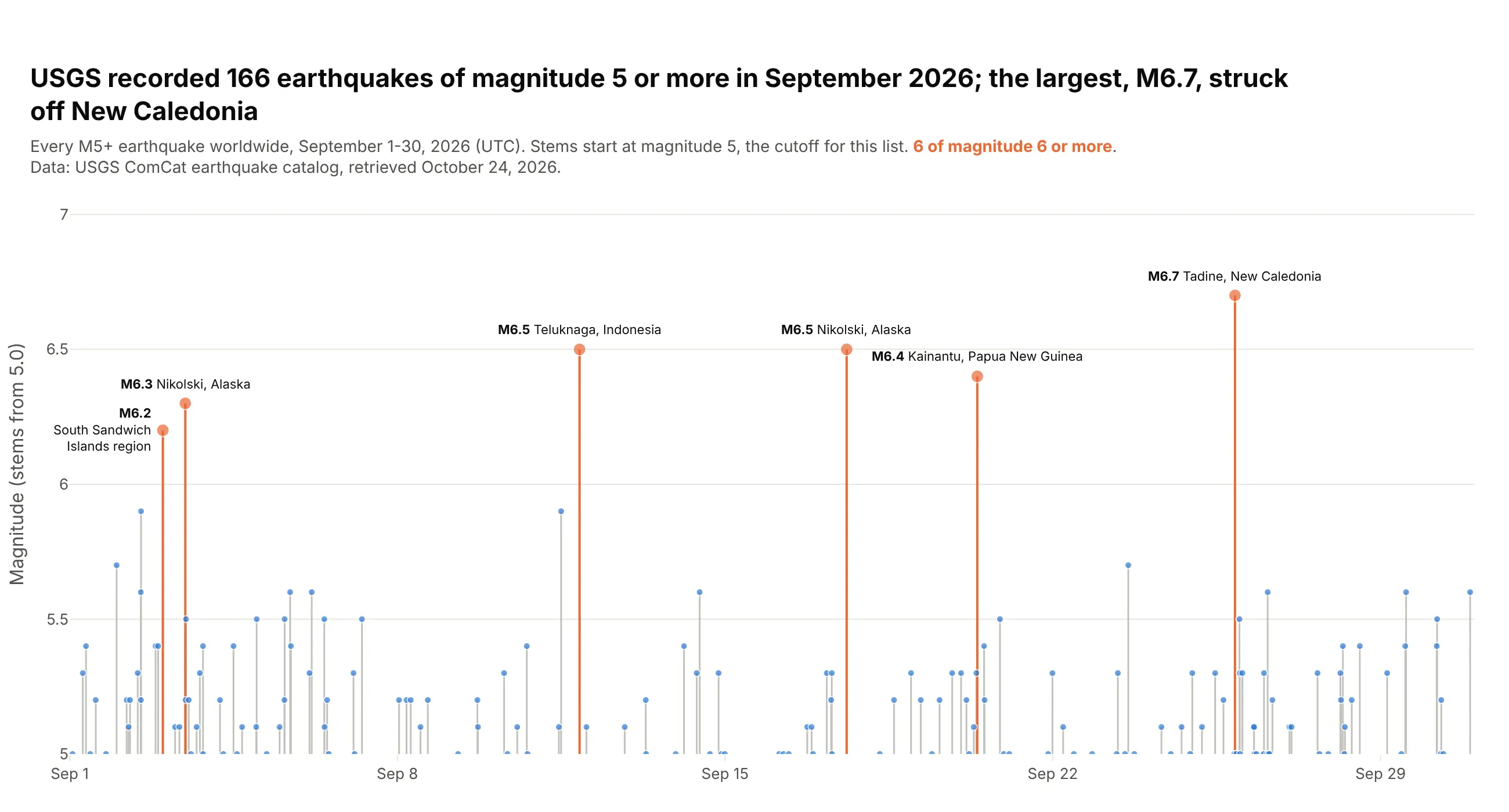
Stem plot of the 166 earthquakes of magnitude 5 or more worldwide in September 2026, each a vertical stem at its time from a magnitude 5 baseline, with the six of M6 or more in orange and labeled, the largest M6.7 near Tadine, New Caledonia on September 25

Events in time, as a stem plot. USGS recorded 166 earthquakes of magnitude 5 or more in September 2026, each drawn as a stem at the moment it happened, and the largest was M6.7 off New Caledonia. Data: USGS ComCat earthquake catalog.

A short history

The lollipop chart grew out of the dot chart, which William Cleveland proposed in 1984 as a more accurate replacement for bar and pie charts (Cleveland, 1984, The American Statistician). His dot charts put one dot per row with a dotted line across the whole row to guide the eye; here is that style redrawn with Plotly on the Phase 3 sponsors (a redraw of the style, not of his original figure):

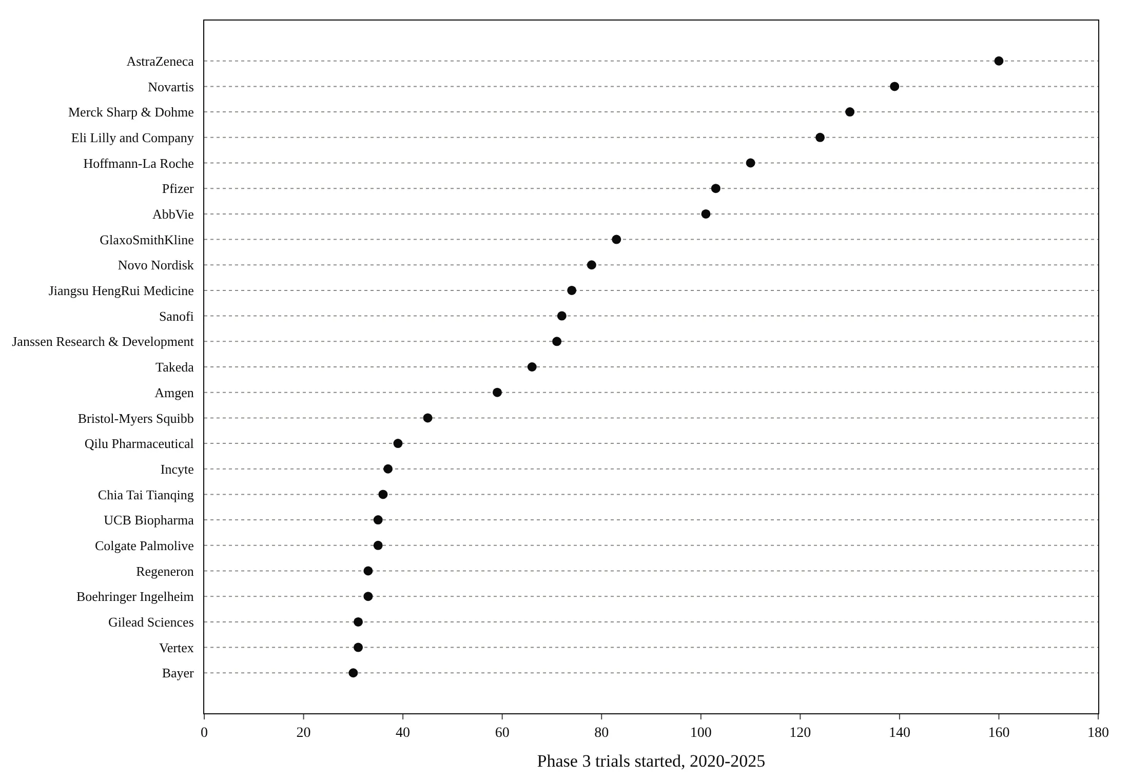
The 25 Phase 3 sponsors drawn as a dot chart in the style of Cleveland's 1984 paper: black dots on dotted lines that run across each row, a box around the plot and serif type, from AstraZeneca (160) to Bayer (30)

His experiments with Robert McGill showed that people judge position along a common scale more accurately than length or area (Cleveland and McGill, 1984). The lollipop keeps the dot and replaces the dotted guide with a stem from zero, so the length reads like a bar again. In signal processing the same chart is called a stem plot.

Alternatives to a lollipop chart

Here are the same 12 sponsors drawn four ways. Some are better for the question, some worse, some just different:

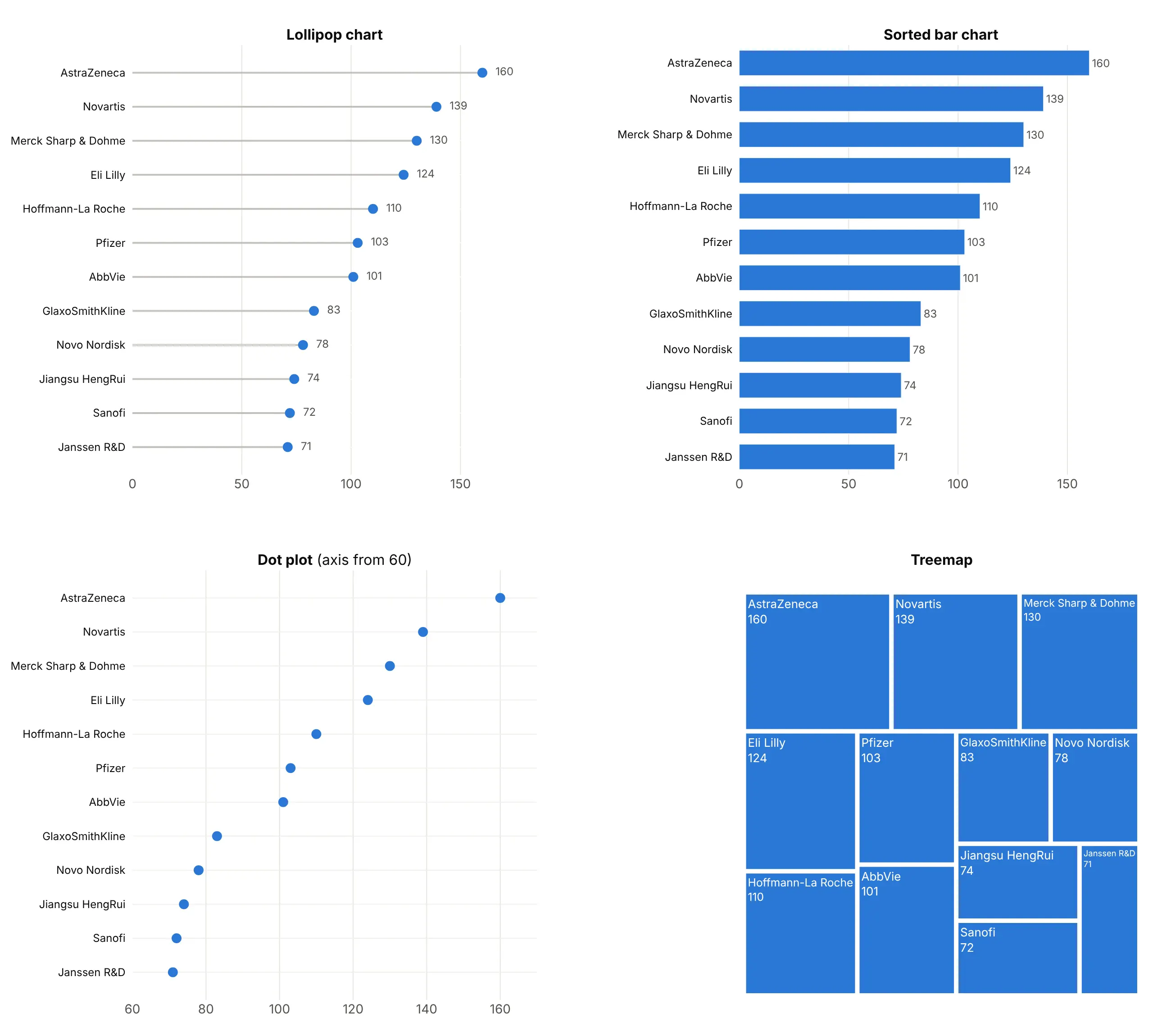
The 12 industry sponsors with the most Phase 3 trials started from 2020 to 2025 drawn as a lollipop chart, a sorted bar chart, a dot plot whose axis starts at 60 and a treemap, from AstraZeneca with 160 trials to Janssen R&D with 71

Sorted bar chart (works too, better for a few bars). It encodes the same length from zero, and with fewer than about ten bars it is just as clear. With 30 or 50 bars of similar length it turns into a block of stripes, which is where the lollipop wins.
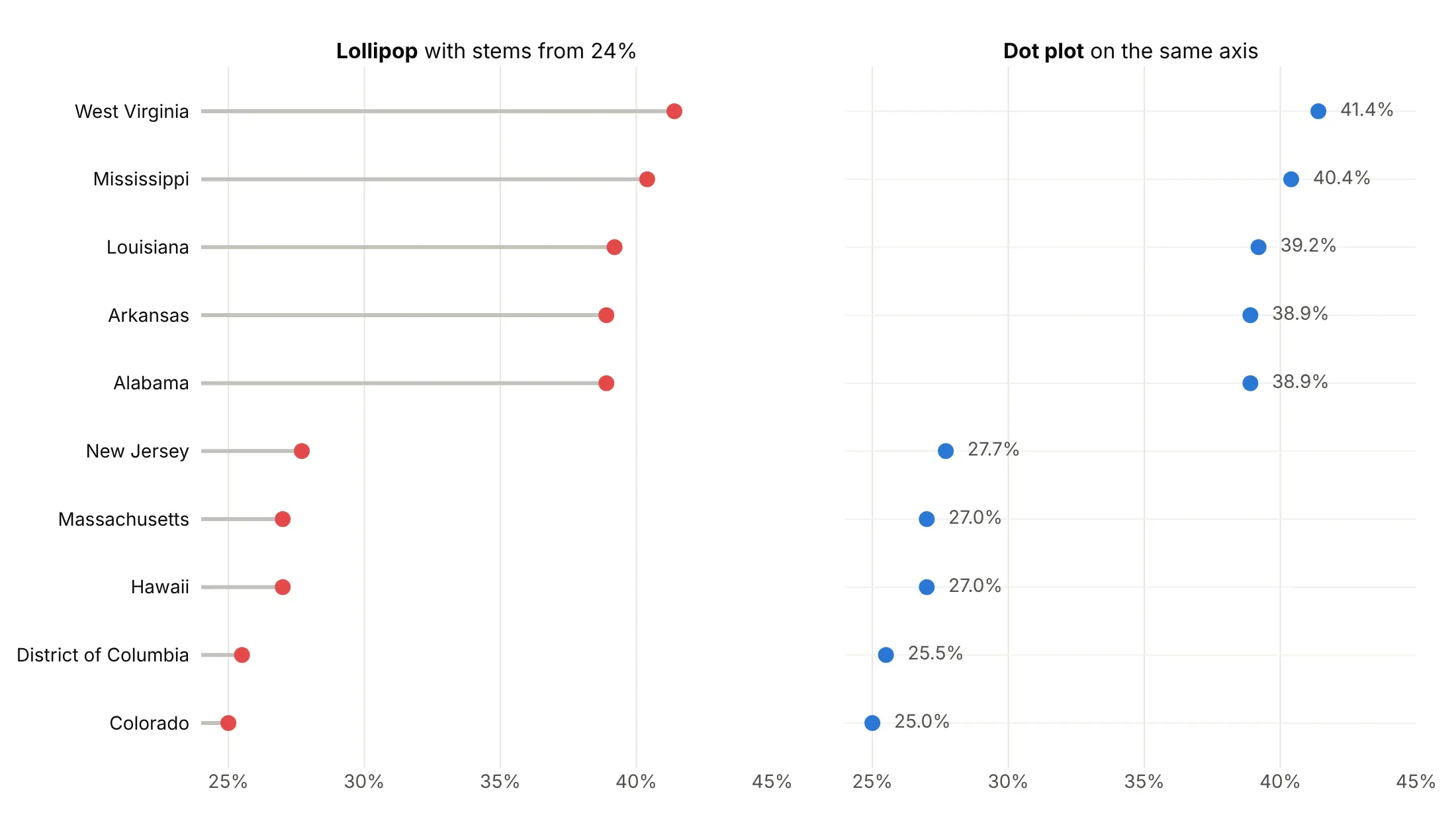
Dot plot (better when you need to zoom). Without stems, the axis can start anywhere, so a dot plot can zoom into 60 to 170 trials or 24% to 45% without exaggerating differences. It loses the length from zero.
Treemap (different). Shows each sponsor as a share of the total, which suits parts of a whole but makes close values hard to compare. See our treemap guide.

For two values per row, such as two years or two groups, use a dumbbell chart instead.

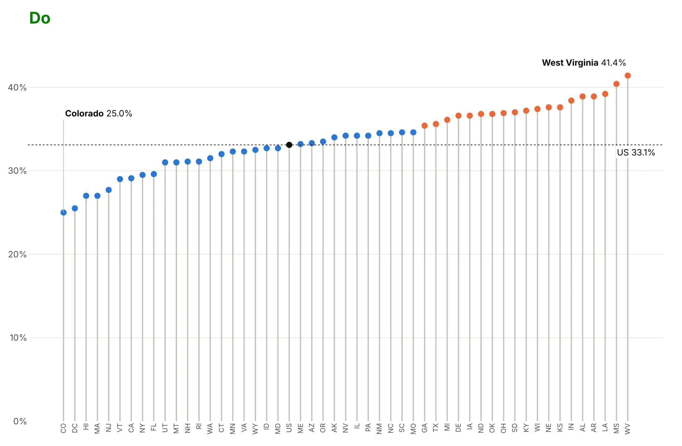
Here's where the dot plot wins. Zoomed into 24% to 45% adult obesity, stems that start at 24% make West Virginia (41.4%) look 17 times Colorado (25.0%), when it is 1.7 times; dots on the same axis don't make that claim:

Two charts of adult obesity in the five lowest and five highest states in 2024 on an axis from 24% to 45%: on the left, lollipop stems from 24% make West Virginia's stem many times longer than Colorado's; on the right, a dot plot shows the same values from 25.0% in Colorado to 41.4% in West Virginia

How to make a lollipop chart

With AI

ChatGPT, Claude Code, GitHub Copilot, Cursor and other AI tools are excellent at writing Plotly code. Name Plotly in the prompt, say where the stems start and how to sort, and list the checks you want:

Make a plotly lollipop chart from inflation.csv (columns: country, iso3, inflation_2024).

- Draw the stems as ONE go.Scatter in mode="lines" with None
  between rows, plus one marker trace for the heads. Don't use add_shape in a loop.
- Stems start at 2% (a dotted reference line labeled "2% target"), not at zero.
- One row per country, sorted by value, highest at the top.
- Orange heads above 2%, blue below; print the value next to each head on the outer side.
- Clip the x axis at 9% and draw any country above it as an arrow with its value.
- A title that states the main takeaway. Assert there are 38 rows and no missing values.
- Save it as lollipop.html and as a PNG at 2x scale.

With Plotly Studio

Plotly Studio is a desktop app where you point an AI at a dataset and it builds charts and a Dash app around your questions. Ask for a lollipop chart the same way:

Show a lollipop chart of 2024 consumer price inflation for the 38 OECD countries, with stems growing from a 2% reference line, sorted by value, orange above 2% and blue below.

Make a lollipop chart in Python or JavaScript

This is the code AI tools write under the hood. In Python, a small helper builds the two traces from a DataFrame, sorts the rows, grows the stems from zero or a benchmark and prints each value on the side its stem points to:

import pandas as pd
import plotly.graph_objects as go


def make_lollipop(df, label, value, base=0, color="#2a78d6",
                  highlight=(), highlight_color="#eb6834", fmt="{:.1f}"):
    d = df.sort_values(value)
    xs, ys = [], []
    for v, c in zip(d[value], d[label]):
        xs += [base, v, None]  # None breaks the line between rows
        ys += [c, c, None]
    colors = [highlight_color if c in highlight else color for c in d[label]]
    sides = ["middle right" if v >= base else "middle left" for v in d[value]]
    fig = go.Figure([
        go.Scatter(x=xs, y=ys, mode="lines", line=dict(color="#c3c2bc", width=2)),
        go.Scatter(x=d[value], y=d[label], mode="markers+text",
                   marker=dict(size=11, color=colors),
                   text=[" " + fmt.format(v) + " " for v in d[value]], textposition=sides),
    ])
    if base:
        fig.add_vline(x=base, line=dict(dash="dot"))
    fig.update_layout(template="simple_white", showlegend=False)
    return fig


df = pd.DataFrame({"country": ["France", "Germany", "India"], "grams": [55.3, 371.3, 713.0]})
make_lollipop(df, "country", "grams", highlight=["India"], fmt="{:.0f} g").show()

In JavaScript, plotly.js takes the same two traces, with null between the rows of the stem trace:

<div id="chart"></div>
<script src="https://cdn.plot.ly/plotly-4.1.1.min.js"></script>
<script>
  const countries = ["France", "Germany", "India"];
  const grams = [55.3, 371.3, 713.0];
  Plotly.newPlot("chart", [
    {
      x: grams.flatMap(v => [0, v, null]),
      y: countries.flatMap(c => [c, c, null]),
      mode: "lines", line: {color: "#c3c2bc", width: 2}, hoverinfo: "skip"
    },
    {
      x: grams, y: countries, mode: "markers+text", marker: {size: 12, color: "#2a78d6"},
      text: grams.map(v => " " + v + " g"), textposition: "middle right"
    }
  ], {showlegend: false});
</script>

For vertical stems, swap x and y. A single marker trace with error bars back to zero, error_y=dict(type="data", symmetric=False, array=up, arrayminus=down, width=0), draws the stems too (example 8).

Share it

Every Plotly chart has a Share chart button (the cloud icon in its toolbar) that uploads it to Plotly Cloud and gives you a link. Only you can see it until you change its visibility.

For a live app, put the chart in a Dash app and publish it with the Plotly Cloud CLI. Coding agents can run these commands for you:

pip install "dash[cloud]"
plotly user login
plotly app publish

If your data has to stay in your own cloud or data center, publish to Dash Enterprise instead.

Dos and don'ts

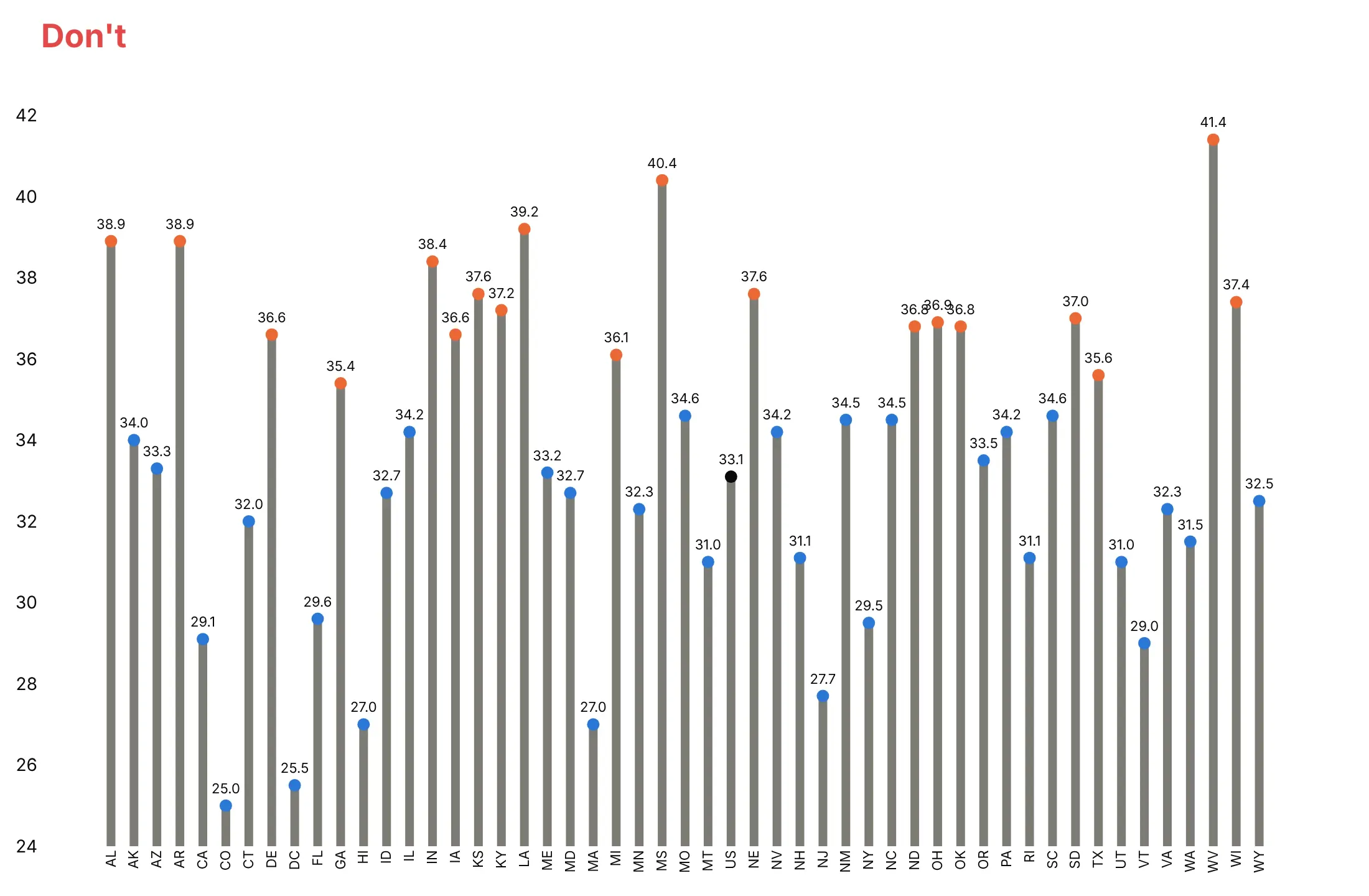
A lollipop chart only works if the stems mean something, so most mistakes are about the baseline, the order and clutter. Here is the same adult obesity data both ways, with the same colors: orange for states at 35% or more, blue for the rest and black for the national value.

Don't start the stems at 24%, keep the states in alphabetical order, draw thick dark stems or print an unformatted number on every head:

A lollipop chart of adult obesity by state with real mistakes: states in alphabetical order, thick dark gray stems that start at 24% so the shortest looks close to zero, an axis without percent signs and a number such as 38.9 printed above every one of the 51 heads

Do sort the states, start the stems at zero, keep them thin and light, and label only the extremes and the national value:

The same lollipop chart with the same colors, sorted from Colorado (25.0%) to West Virginia (41.4%), thin light gray stems from 0%, percent signs on the axis and a dotted line for the US at 33.1%

Choose the baseline and the color

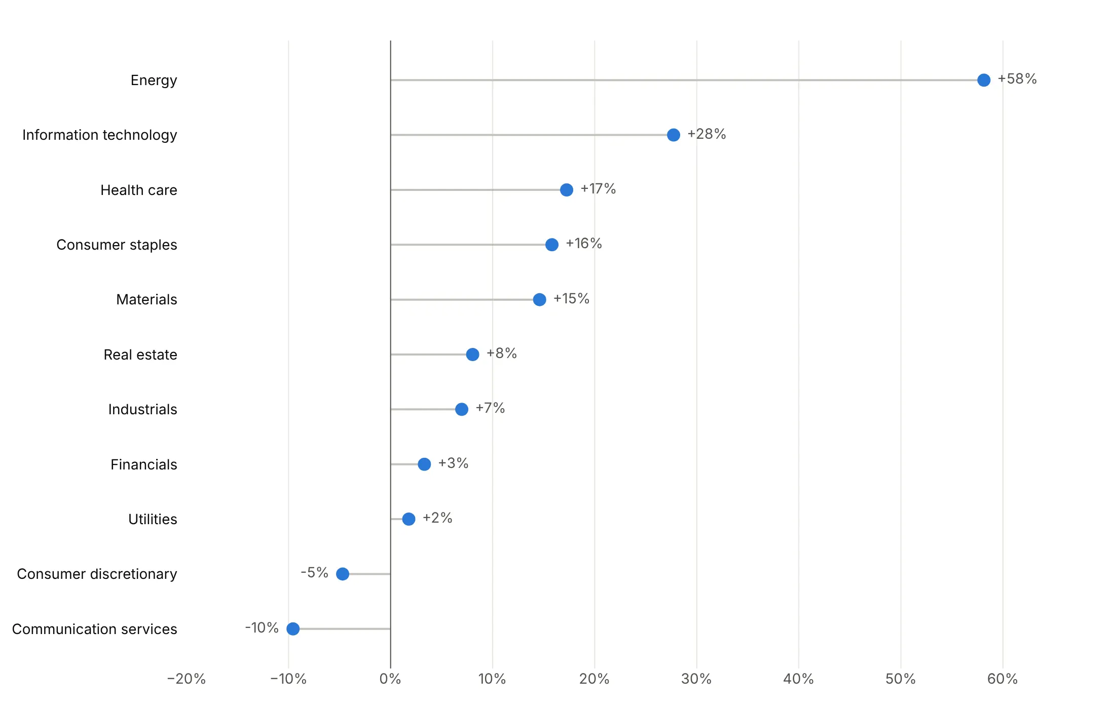
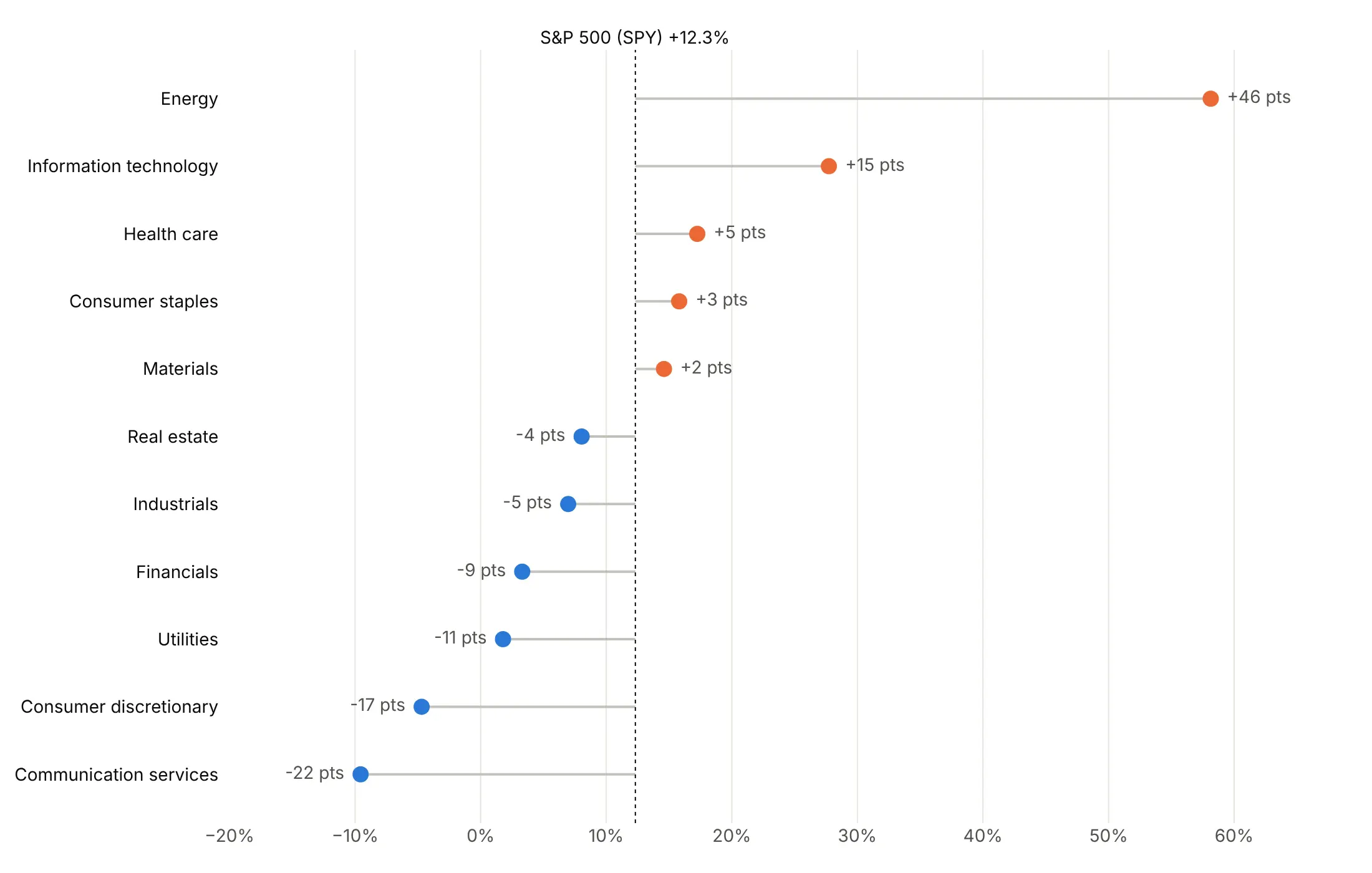
The baseline and the colors decide what the chart says. Here are four options on the 2026 returns of the 11 S&P 500 sectors.

Plain and sorted. Stems from zero in one color show the ranking and the sign, and it's a good default.

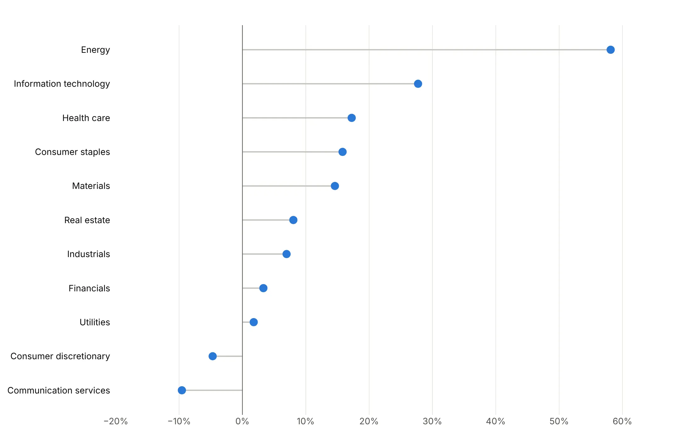
The 11 S&P 500 sector returns of 2026 as a sorted lollipop chart with stems from zero in one blue, from Energy at the top to Communication services below zero

Values at the head. Printing each return on the outer side saves readers from reading the axis.

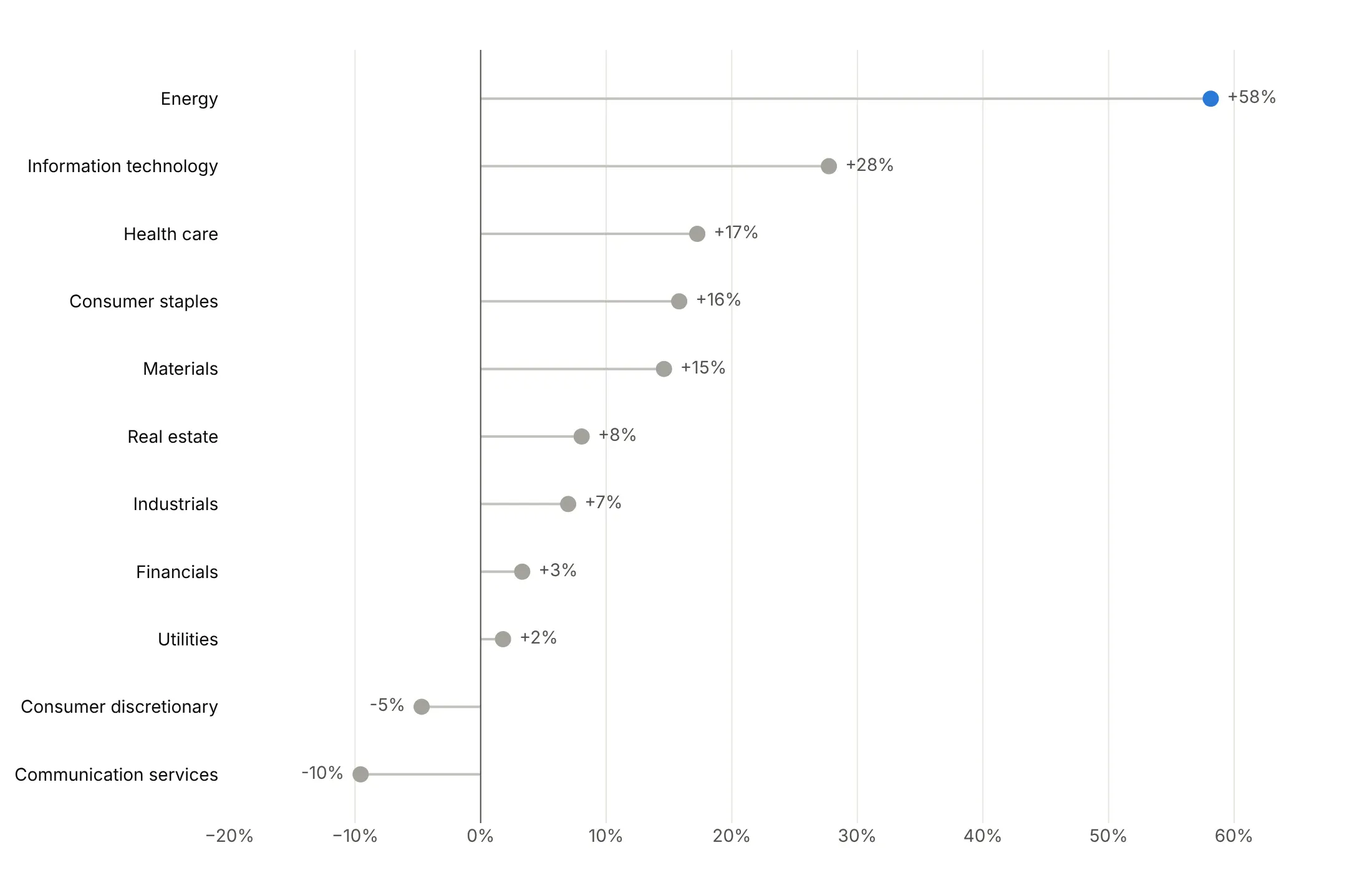
The same sector returns with each value printed beside its head, from +58% for Energy to -10% for Communication services

Stems from a benchmark. Starting the stems at the market's 12.3% turns the chart into "beat the market or not": five sectors did, led by Energy at 46 points above.

The same sector returns with stems growing from a dotted line at the S&P 500's +12.3%, orange for the five sectors above it and blue for the six below, labeled from +46 pts for Energy to -22 pts for Communication services

Highlight one story. Energy is the only color and every other sector is gray.

The same sector returns with Energy (+58%) in blue and every other sector in gray

Checklist

Write a title that states the takeaway.
Sort by value, unless the categories have a natural order (months, versions, league positions).
Start stems at zero, or at a benchmark you name on the chart.
Keep stems thin and light gray (1 to 3 px) and heads 8 to 14 px.
Print values on the side the stem points to, or label only the ones that matter.
Clip the axis for one extreme outlier and mark it with an arrow and its value.

Don't

Start stems at an arbitrary value or use them on a log axis; use a dot plot instead.
Draw stems with fig.add_shape() in a loop.
Give every row its own color or add a legend for rows that are already labeled.
Use a lollipop for two values per row; use a dumbbell chart.

Options to customize

These are the go.Scatter and layout options that build a lollipop chart. The full list is in the Plotly scatter reference.

mode="lines" with None in x and y: one trace draws every stem; None breaks the line between rows.
mode="markers" or "markers+text": the heads, with or without printed values.
line.color, line.width: keep stems light gray and 1 to 3 px.
marker.color, marker.size as lists: one color or size per row, for a highlight, a sign or a second variable.
marker.symbol: "arrow-right" for an outlier drawn off the scale.
text, texttemplate, textposition: values at the heads; textposition can be a list, left for negative stems and right for positive.
error_x, error_y with symmetric=False, array, arrayminus, width=0: error bars as stems on a single marker trace (one stem color).
yaxis.categoryorder="array", categoryarray: fix the row order, sorted or natural.
fig.add_vline, fig.add_hline: the benchmark or zero line.
xaxis.range: clip the axis so one outlier doesn't flatten the rest.
make_subplots(rows, cols, shared_xaxes=True): panels for groups or more than about 50 rows.
hovertemplate, customdata: counts or extra columns on hover.

More lollipop chart examples

Eight more lollipop charts built from real public data, each with its source, the technique that makes it work and a prompt to rebuild it.

1. Adverse event reports for four GLP-1 drugs

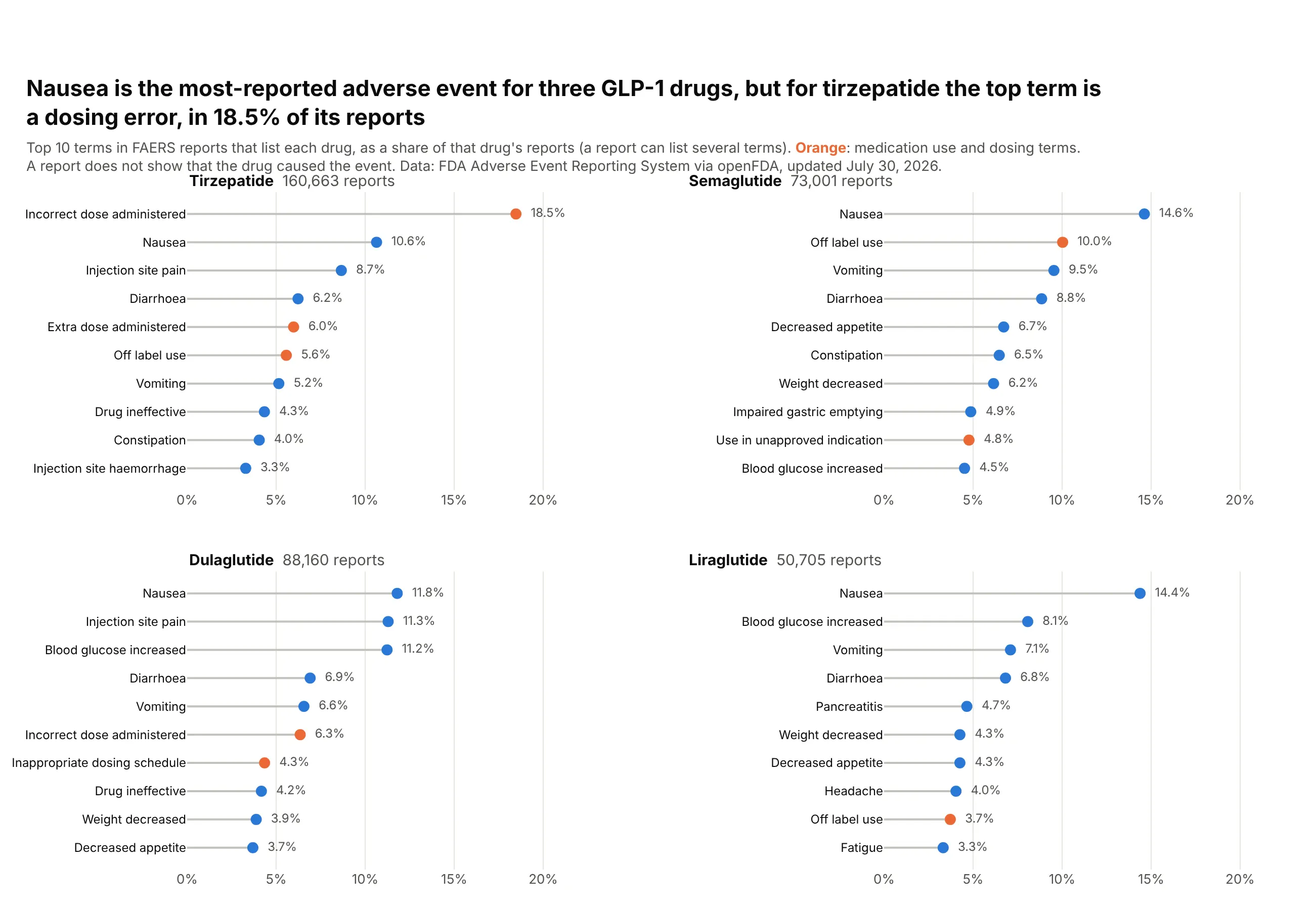
Four lollipop charts of the 10 most-reported FAERS terms for tirzepatide, semaglutide, dulaglutide and liraglutide as a share of each drug's reports. Nausea leads for semaglutide (14.6%), liraglutide (14.4%) and dulaglutide (11.8%); for tirzepatide the top term is incorrect dose administered, 18.5% of 160,663 reports

Nausea is the most-reported adverse event term for semaglutide, liraglutide and dulaglutide. For tirzepatide, the top term is "incorrect dose administered", in 18.5% of its 160,663 FAERS reports. Reports show what was reported, not what the drug caused. Data: FDA Adverse Event Reporting System via openFDA.

Tip: small multiples with a shared x axis compare shares across drugs, while each panel keeps its own sort.

Get the data from the openFDA drug adverse event API (FDA Adverse Event Reporting System):
for semaglutide, tirzepatide, liraglutide and dulaglutide, the number of reports listing the drug
(patient.drug.openfda.generic_name) and the top 10 counts of patient.reaction.reactionmeddrapt.exact
and shape it into a table (columns: drug, reports, term, count, pct_of_reports, rank).

Build a 2x2 plotly lollipop chart, one panel per drug, sorted within each panel.
- Stems as one go.Scatter with None gaps per panel; shared x axis in % of reports.
- Orange heads for dosing and off-label terms, blue for the rest; print the share at each head.
- Panel titles with the drug name and its number of reports.

2. Adult obesity by state

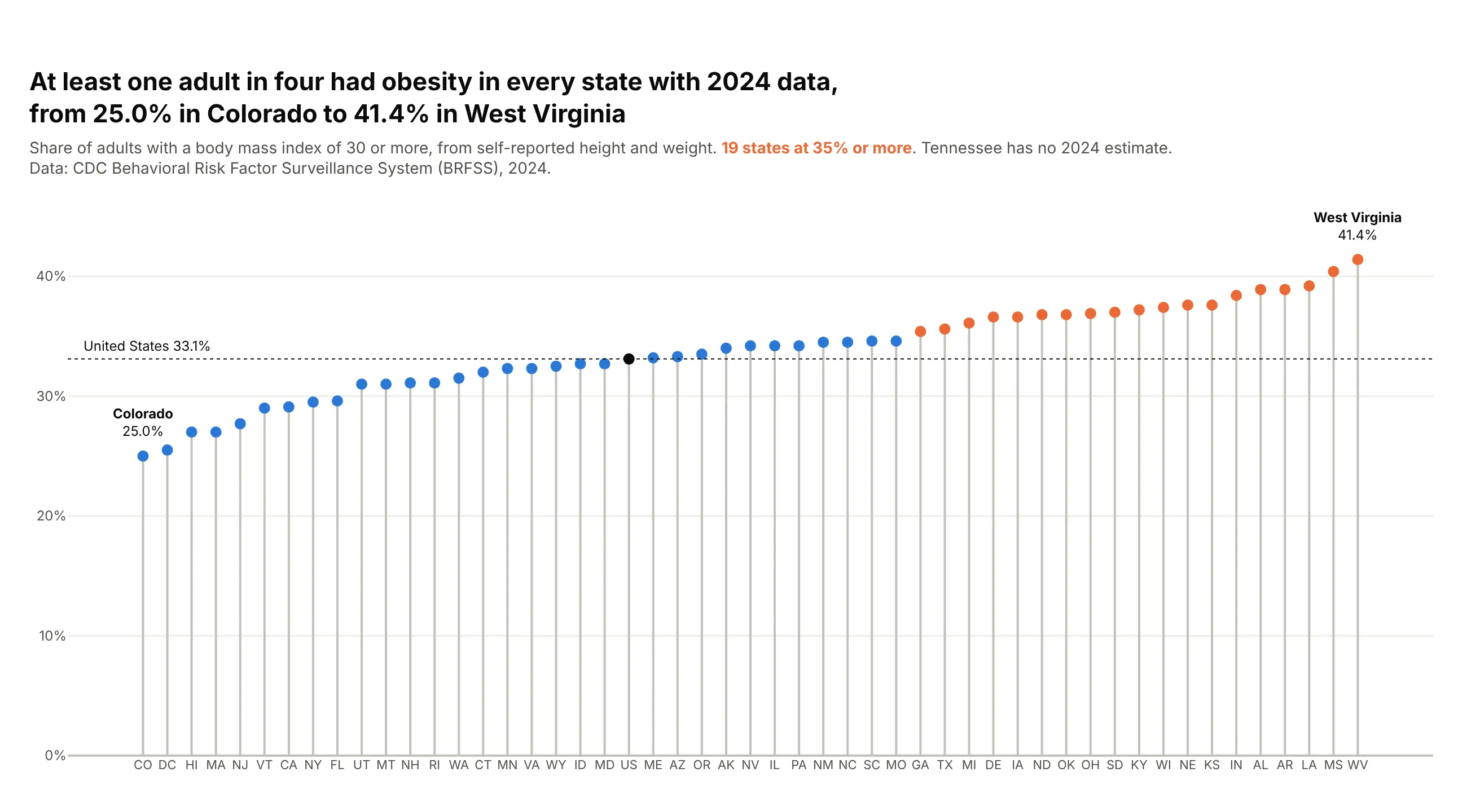
Vertical lollipop chart of the share of adults with obesity in 2024 for 49 states and DC, sorted from 25.0% in Colorado to 41.4% in West Virginia, with the 19 states at 35% or more in orange and the national value of 33.1% as a black stem and dotted line

At least one adult in four had obesity in every state with 2024 data, from 25.0% in Colorado to 41.4% in West Virginia. Nineteen states were at 35% or more, and the national figure was 33.1%. Data: CDC Behavioral Risk Factor Surveillance System (BRFSS).

Tip: with 50 values between 24% and 42%, thin vertical stems with state codes avoid the striped block that 50 bars make.

Get the data from CDC's "Nutrition, Physical Activity, and Obesity - Behavioral Risk Factor
Surveillance System" dataset on data.cdc.gov (hn4x-zwk7), question Q036, overall stratum, 2024
and shape it into a table (columns: state, code, pct, low, high), states, DC and the national row.

Build a vertical plotly lollipop chart: state codes on x, sorted by pct, stems from 0.
- Orange heads at 35% or more, blue below, the national value in black with a dotted line.
- Label the lowest and highest states above their heads.

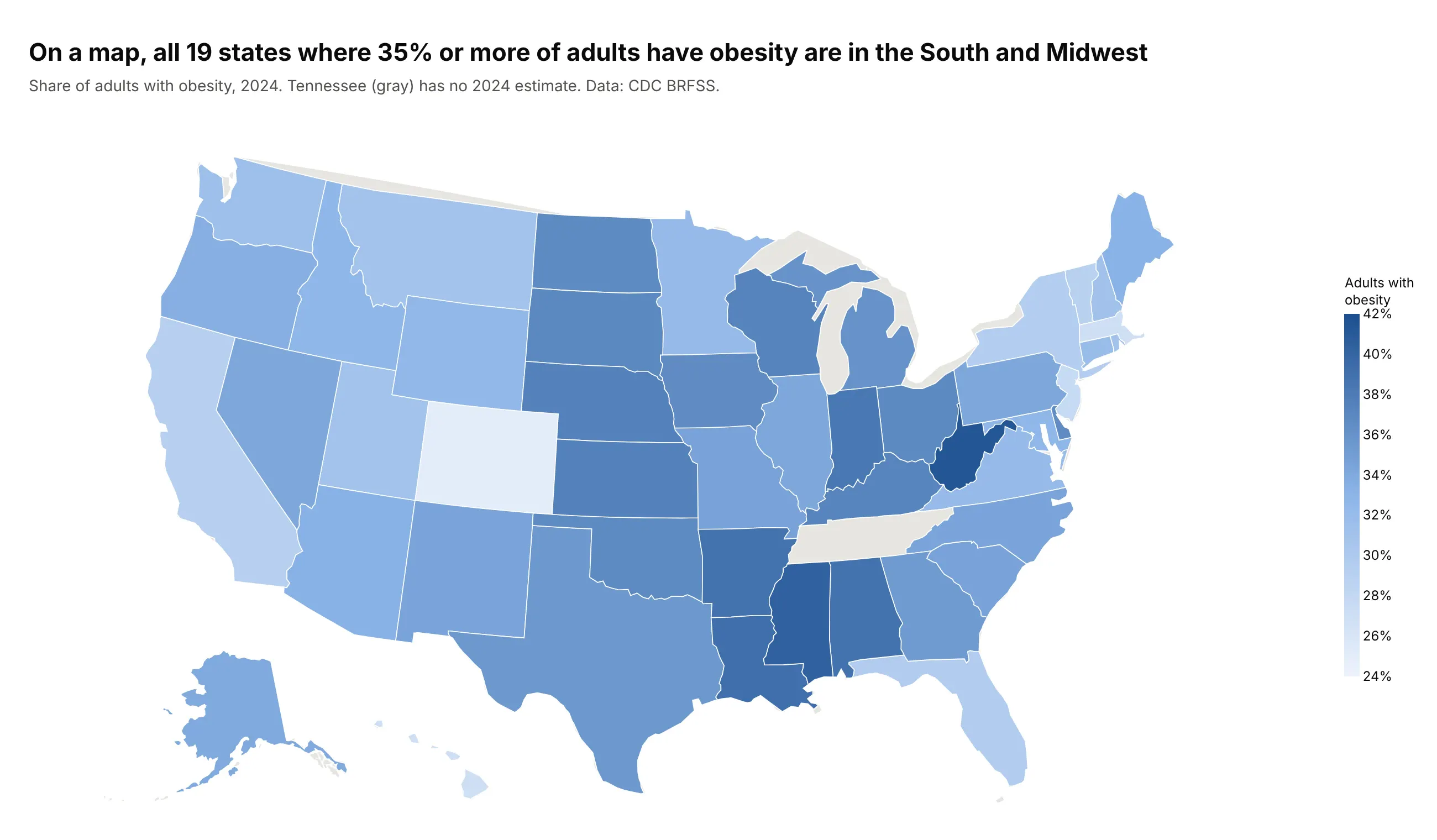
Another way to see it: a choropleth map shows that all 19 states at 35% or more are in the South and Midwest, but it hides how close most states are to each other.

Choropleth map of adult obesity by state in 2024, darkest in West Virginia, Mississippi, Louisiana and the Midwest, lightest in Colorado, with Tennessee in gray for no data

3. The 2026 returns of the S&P 500 sectors

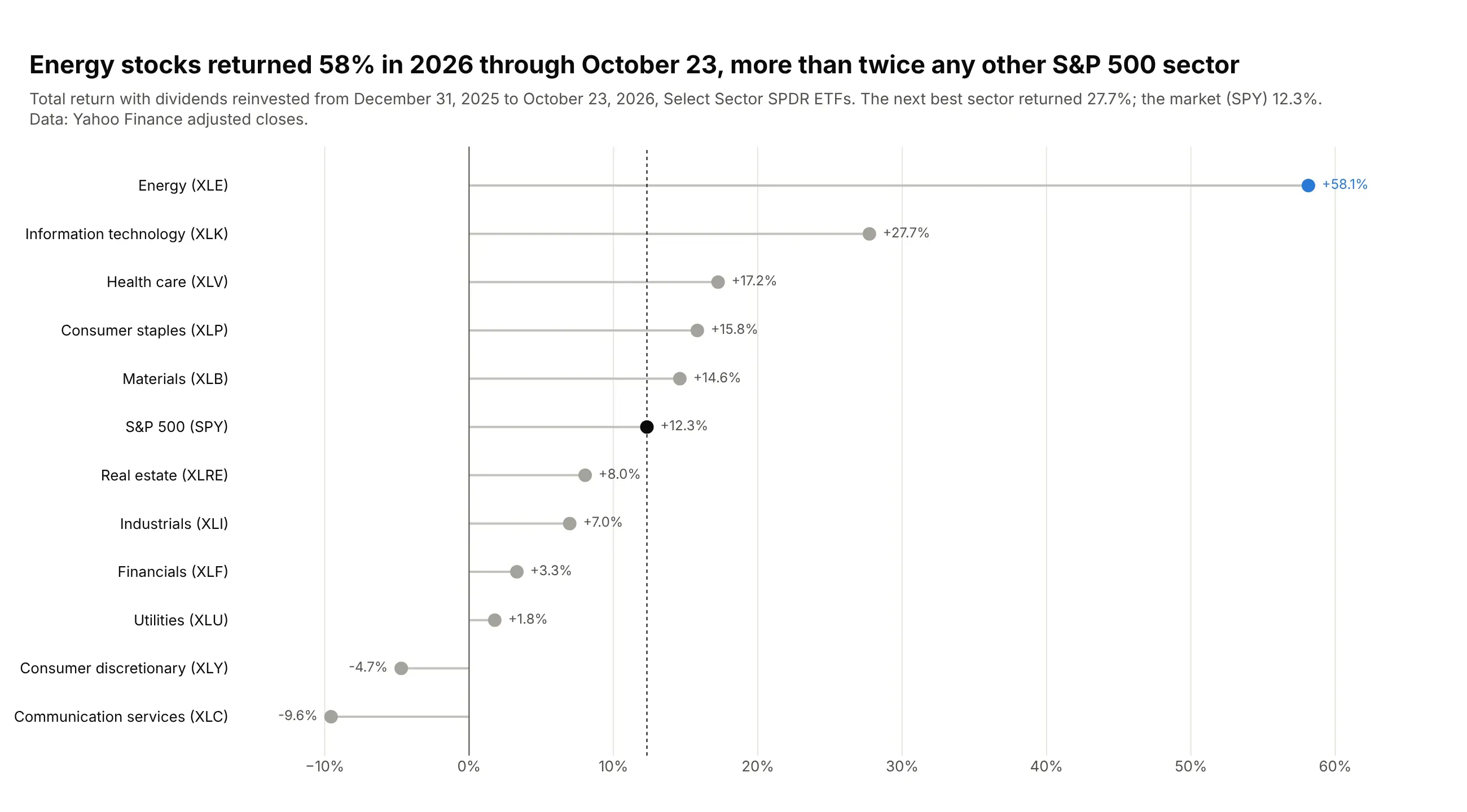
Lollipop chart of the 2026 year-to-date total return of the 11 Select Sector SPDR ETFs and SPY through October 23: Energy +58.1% in blue, Information technology +27.7%, SPY +12.3% in black with a dotted line, and Communication services -9.6%, the rest in gray

Energy stocks returned 58% in 2026 through October 23, more than twice the next best sector, information technology (27.7%). The market as a whole (SPY) returned 12.3%, and communication services lost 9.6%. Data: Yahoo Finance adjusted closes of the Select Sector SPDR ETFs.

Tip: when the chart is about one row, gray out the rest and give the reference row its own color.

Get the data from Yahoo Finance's chart API: daily adjusted closes for XLE, XLB, XLI, XLY, XLP,
XLV, XLF, XLK, XLC, XLU, XLRE and SPY
and shape it into a table (columns: sector, ticker, start_date, end_date, return_pct)
with the total return from 2025-12-31 to the latest close.

Build a horizontal plotly lollipop chart sorted by return, stems from 0.
- Energy in blue, SPY in black with a dotted line at its value, everything else gray.
- Print "+58.1%" on the outer side of each head.

4. The carbon intensity of electricity

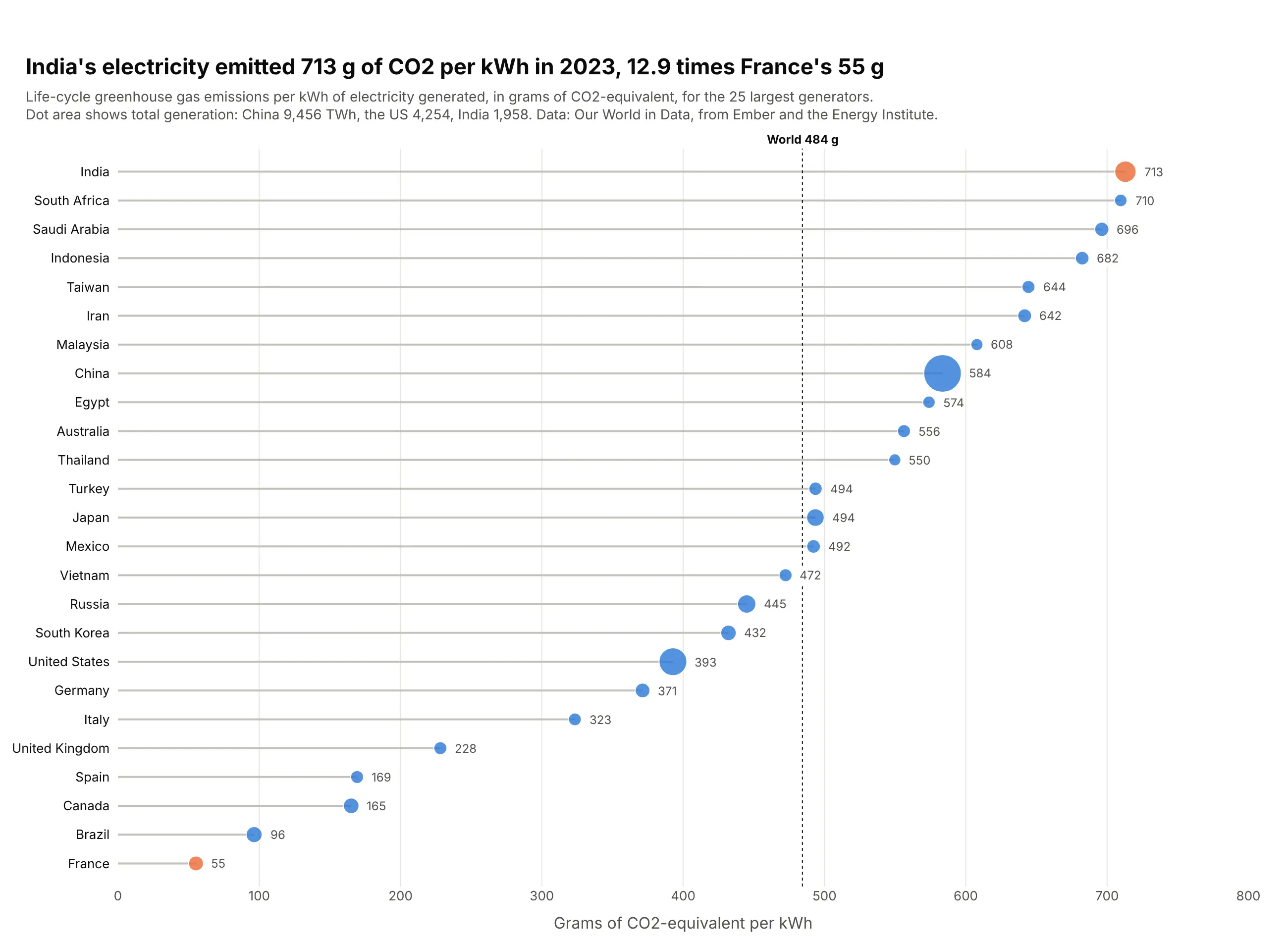
Lollipop chart of the carbon intensity of electricity in 2023 for the 25 largest generators, with heads sized by generation: India 713 g of CO2 per kWh and France 55 g in orange, China (584 g, 9,456 TWh) and the US (393 g, 4,254 TWh) as the largest heads, and the world average at 484 g

Each kWh of India's electricity came with 713 g of CO2-equivalent in 2023, 12.9 times France's 55 g. China, which generates the most electricity by far (9,456 TWh), was at 584 g, above the world's 484 g. Data: Our World in Data, from Ember and the Energy Institute.

Tip: size the heads by a second variable (generation) with area proportional to the value, and keep the stems the same for every row.

Get the data from Our World in Data's energy dataset (owid-energy-data.csv), carbon_intensity_elec
and electricity_generation, 2023, countries only
and shape it into a table (columns: country, iso_code, generation_twh, intensity_g_kwh, year).
Keep the 25 largest generators.

Build a horizontal plotly lollipop chart sorted by intensity.
- Head area proportional to generation (size = a + b * sqrt(twh / max)); India and France in orange.
- Print the value beyond each head; dotted line at the world value, 484 g/kWh.

5. How US electricity generation changed since 2016

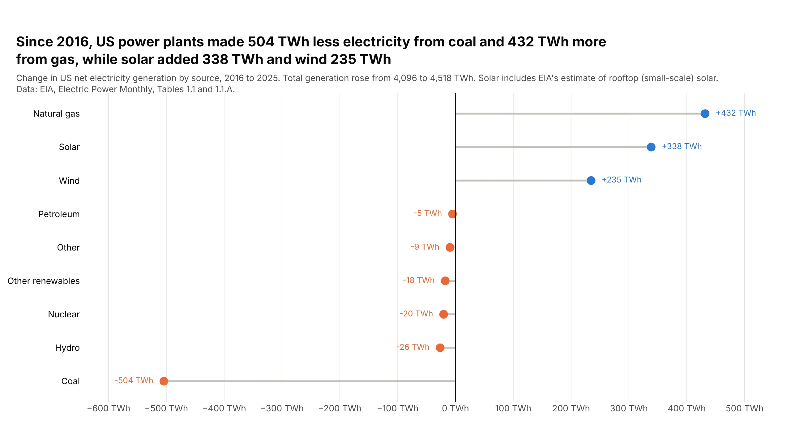
Diverging lollipop chart of the change in US net electricity generation by source from 2016 to 2025: natural gas +432 TWh, solar +338 and wind +235 in blue, and coal -504, hydro -26, nuclear -20 and others in orange

US power plants made 504 TWh less electricity from coal in 2025 than in 2016, and 432 TWh more from natural gas. Solar added 338 TWh and wind 235, while total generation rose from 4,096 to 4,518 TWh. Data: EIA, Electric Power Monthly, Tables 1.1 and 1.1.A.

Tip: for a diverging lollipop, put each label on the side the stem points to and color by sign.

Get the data from EIA's Electric Power Monthly, Table 1.1 (net generation by energy source) and
Table 1.1.A (renewable sources), annual totals for 2016 and 2025, thousand MWh converted to TWh
and shape it into a table (columns: source, twh_2016, twh_2025, change_twh) with coal, natural gas,
nuclear, hydro, wind, solar (including small-scale), petroleum, other renewables and other.

Build a horizontal plotly lollipop chart of change_twh sorted by change, stems from 0.
- Blue heads for gains, orange for losses; print "+432 TWh" on the outer side.

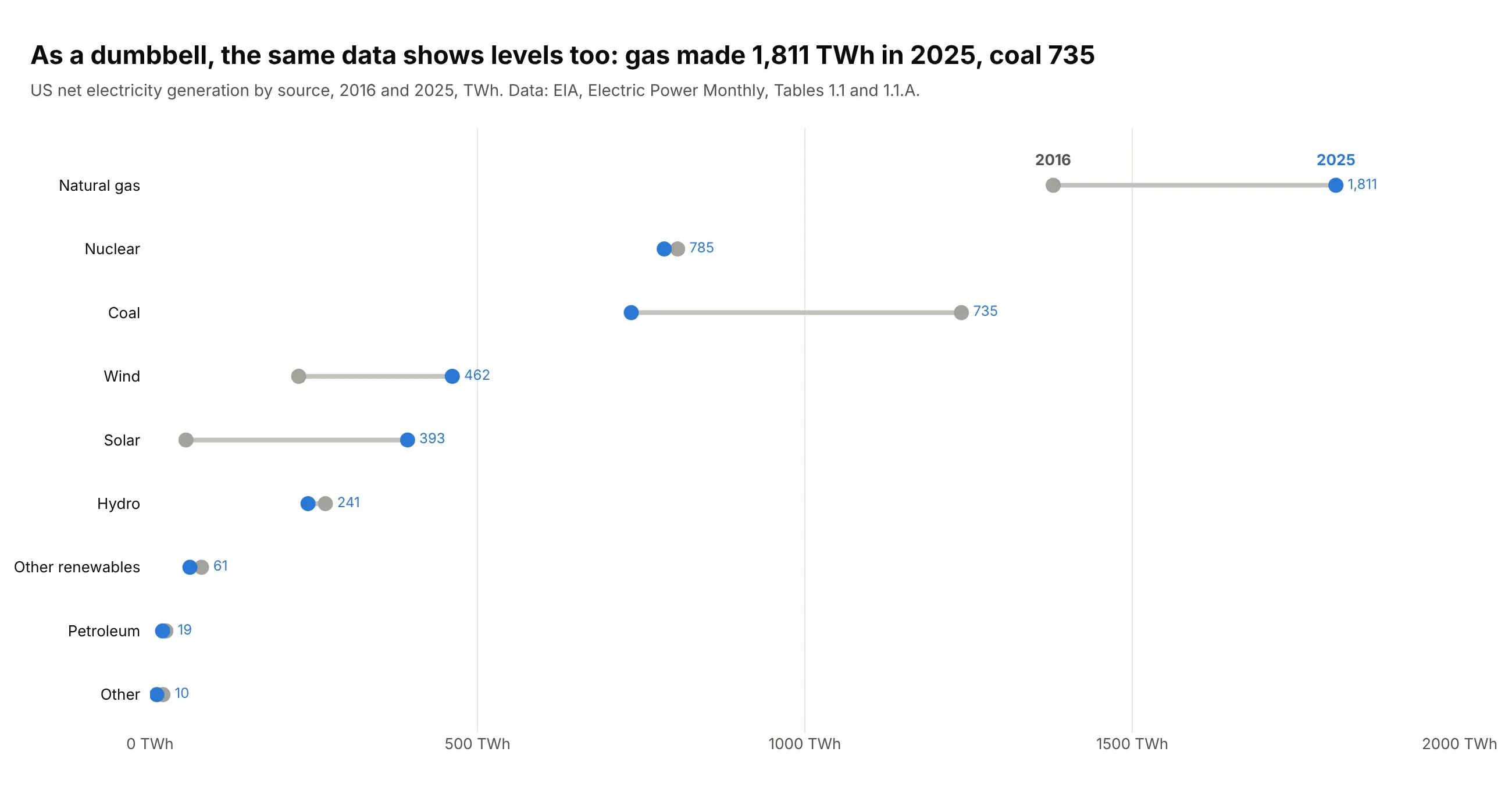
Another way to see it: a dumbbell chart of the two years shows the levels too, with gas at 1,811 TWh and coal at 735 TWh in 2025, but small changes such as nuclear's collapse into one dot.

Dumbbell chart of US net generation by source in 2016 and 2025, from natural gas 1,379 to 1,811 TWh and coal 1,239 to 735 TWh to petroleum 24 to 19 TWh

6. How hard each kind of power plant runs

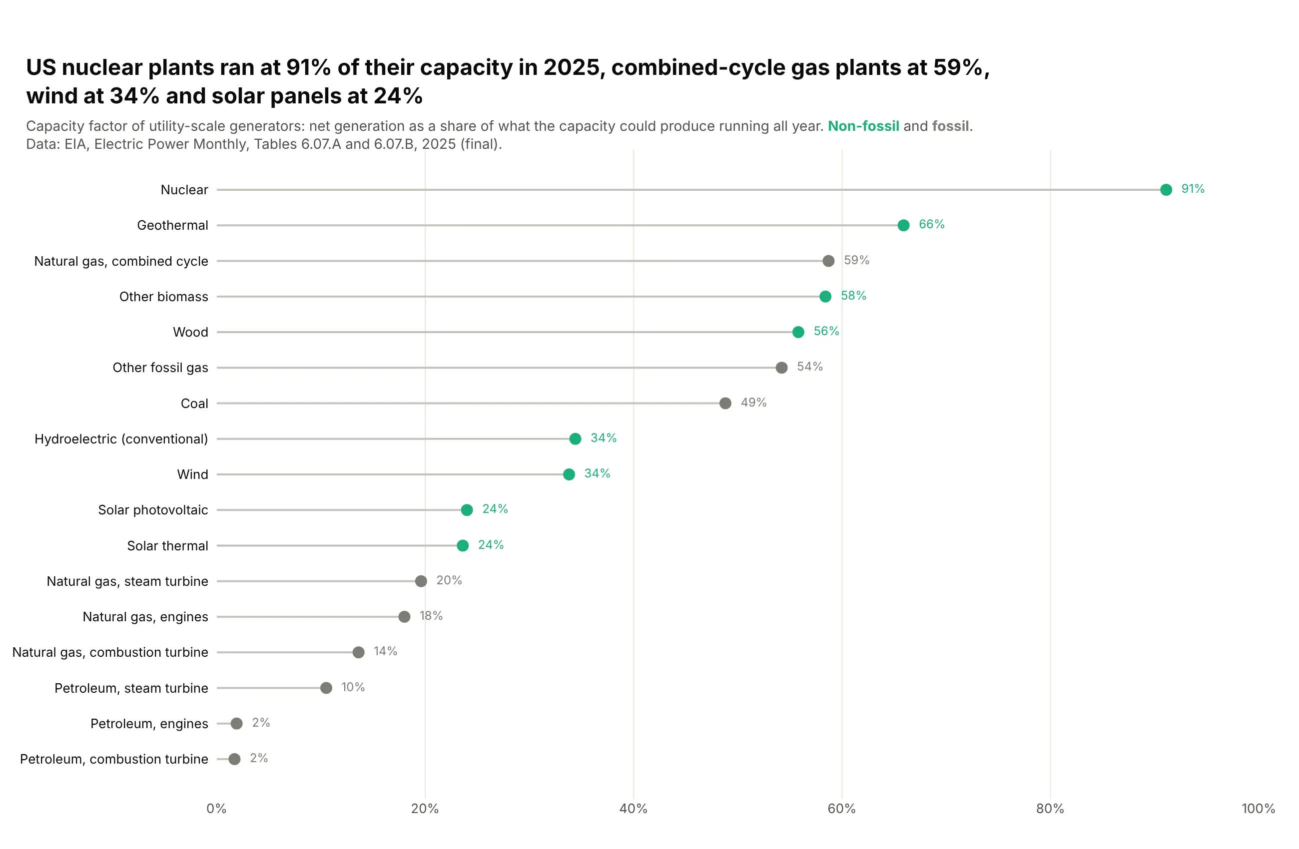
Lollipop chart of 2025 capacity factors of US utility-scale generators on a 0-100% axis: nuclear 91%, geothermal 66%, combined-cycle gas 59%, coal 49%, hydro and wind 34%, solar photovoltaic 24% and petroleum combustion turbines 2%, with non-fossil heads in green and fossil in gray

US nuclear plants produced 91% of what their capacity could make running all year in 2025, combined-cycle gas plants 59%, wind 34% and solar panels 24%. Gas and oil peaking turbines ran at 2% to 14%. Data: EIA, Electric Power Monthly, Tables 6.07.A and 6.07.B.

Tip: for a bounded rate, fix the axis at 0 to 100% so every stem is read against the same ceiling.

Get the data from EIA's Electric Power Monthly, Tables 6.07.A and 6.07.B (capacity factors of
utility-scale generators), the 2025 annual row
and shape it into a table (columns: technology, fuel_group, capacity_mw, capacity_factor_pct).

Build a horizontal plotly lollipop chart sorted by capacity factor, x axis fixed at 0-100%.
- Green heads for non-fossil, gray for fossil; print the percentage in the head's color.

7. Population change by state, grouped by region

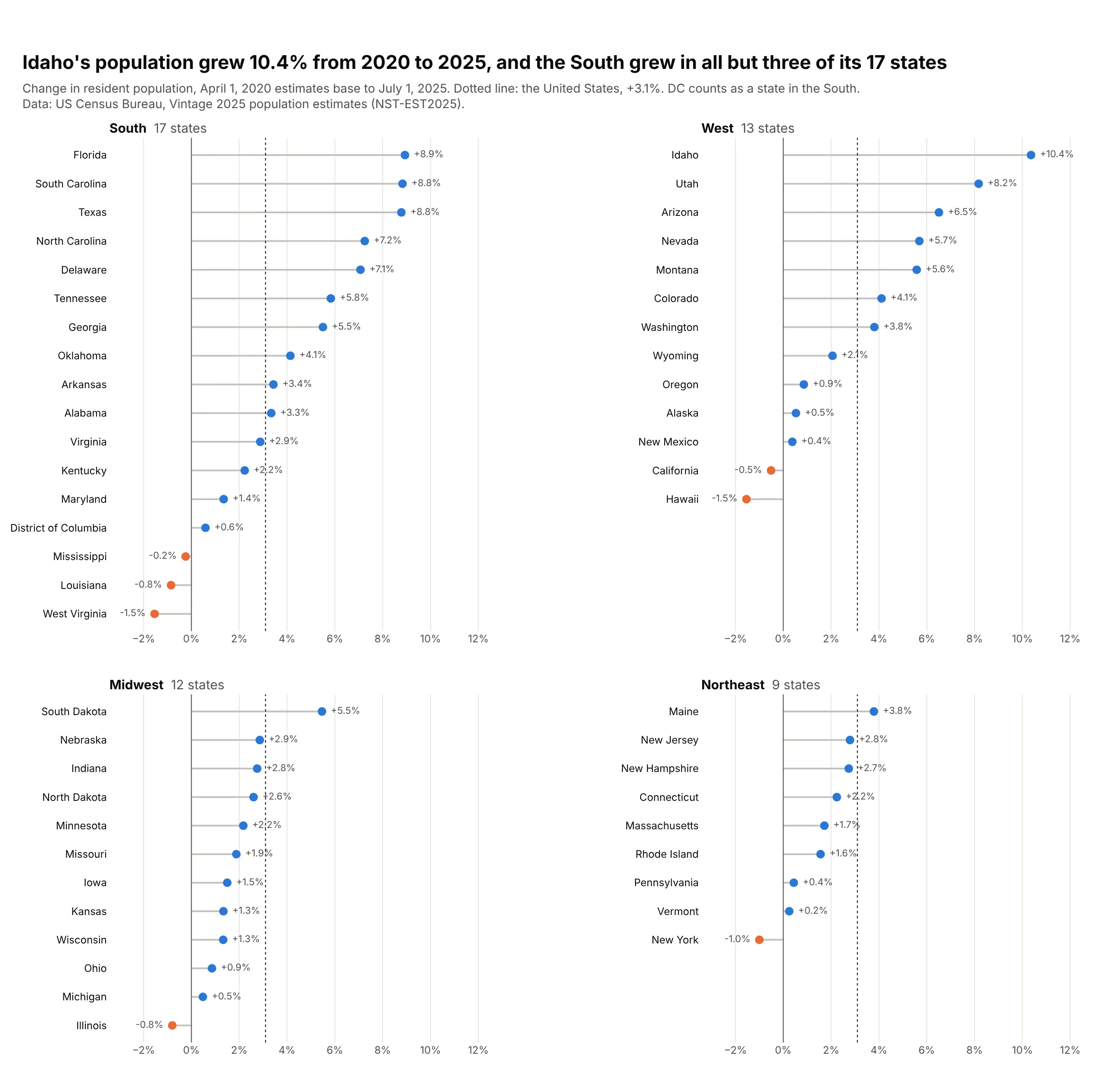
Four lollipop panels of the population change from April 2020 to July 2025 for the states of the South, West, Midwest and Northeast, sorted within each region, with gains in blue and losses in orange: Idaho +10.4% and Florida +8.9% lead, and West Virginia and Hawaii (-1.5%) and New York (-1.0%) fell; a dotted line marks the US at +3.1%

Idaho's population grew 10.4% from 2020 to 2025, the most of any state, and the South grew in 14 of its 17 states. Seven states shrank, led by West Virginia and Hawaii (-1.5% each); the US grew 3.1%. Data: US Census Bureau, Vintage 2025 population estimates.

Tip: split long lists into panels by a natural group and repeat the national reference line in each.

Get the data from the Census Bureau's Vintage 2025 state population estimates
(NST-EST2025-ALLDATA.csv), ESTIMATESBASE2020, POPESTIMATE2025 and REGION
and shape it into a table (columns: state, region, base_2020, pop_2025, change_pct), plus a US row.

Build a 2x2 plotly lollipop chart, one panel per Census region, sorted within each panel.
- Blue heads for growth, orange for decline; values on the outer side; shared x axis.
- Dotted line at the US change in every panel; panels aligned to the top.

8. Premier League goal difference in table order

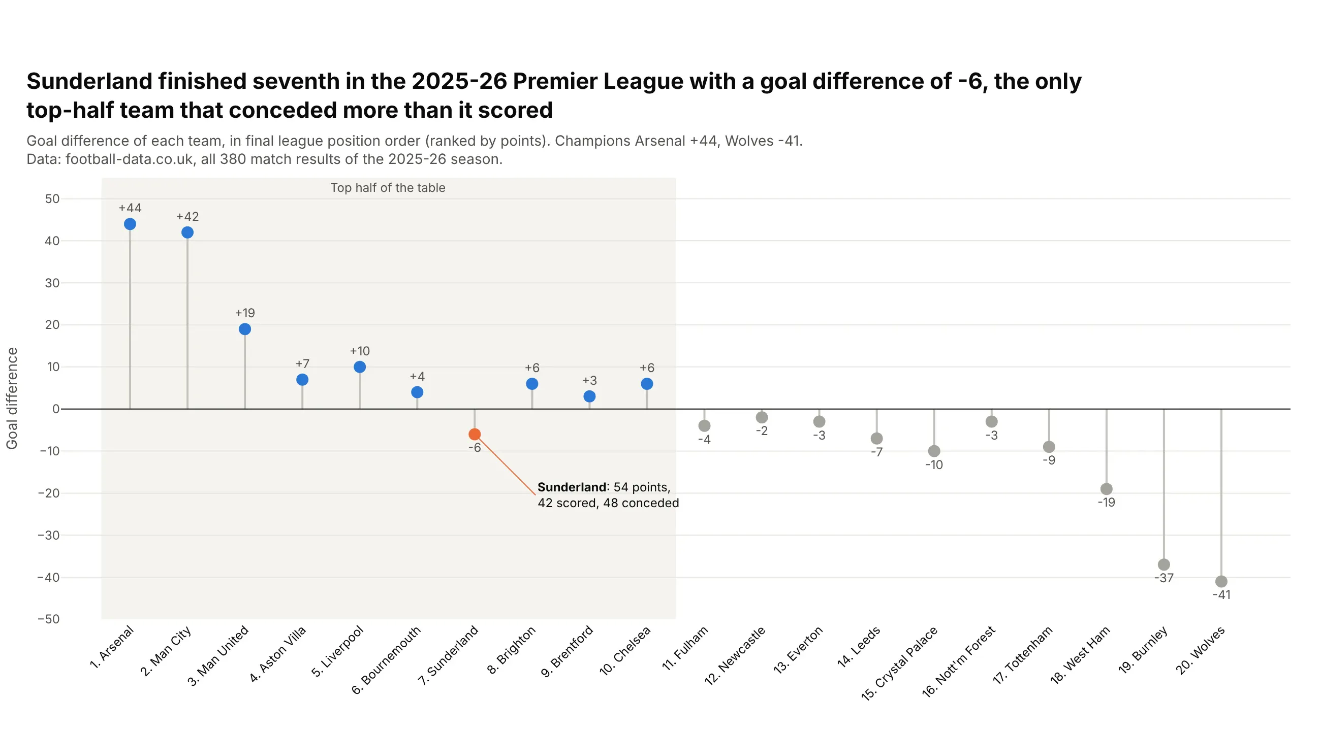
Vertical lollipop chart of goal difference for the 20 Premier League teams in 2025-26 in final table order, from Arsenal +44 and Man City +42 to Wolves -41, with the top half shaded and Sunderland, 7th with -6, in orange

Sunderland finished seventh in the 2025-26 Premier League with a goal difference of -6, the only top-half team that conceded more than it scored. Champions Arsenal had +44 and Wolves -41. Data: football-data.co.uk, all 380 match results.

Tip: keep the table order instead of sorting by value, and draw the stems as error bars on one marker trace.

Get the data from football-data.co.uk, English Premier League 2025-26 results (E0.csv, FTHG and FTAG)
and shape it into a final table (columns: pos, team, played, won, drawn, lost, gf, ga, gd, points),
ranked by points, then goal difference, then goals scored.

Build a vertical plotly lollipop chart with teams on x in table order.
- One marker trace; stems from error_y with array/arrayminus back to 0 and width=0.
- Shade the top half; Sunderland in orange with an annotation of points, scored and conceded.