Image Plots with imshow - A Complete Guide

TL;DR

• An image plot draws a grid of numbers as a grid of colored pixels at their true shape: a photograph's red, green and blue values as a color picture, or one measurement per pixel (elevation, brightness, vegetation) through a color scale.
• Image plots are also known as imshow plots, after the function in matplotlib and Plotly, and for small matrices as matshow plots. They are similar to heatmaps and contour plots.
• In Plotly, px.imshow handles both kinds: it draws three-channel arrays as an image trace and single-channel arrays as a heatmap trace, keeps pixels square, and puts row 0 at the top unless you set origin="lower".
• The settings that matter are the contrast (zmin and zmax, or a log scale), the coordinates (x, y and origin), binary_string=True for images of millions of pixels, and facet_col or animation_frame for stacks and time series of images.

What is an image plot?

Image plots look like this:

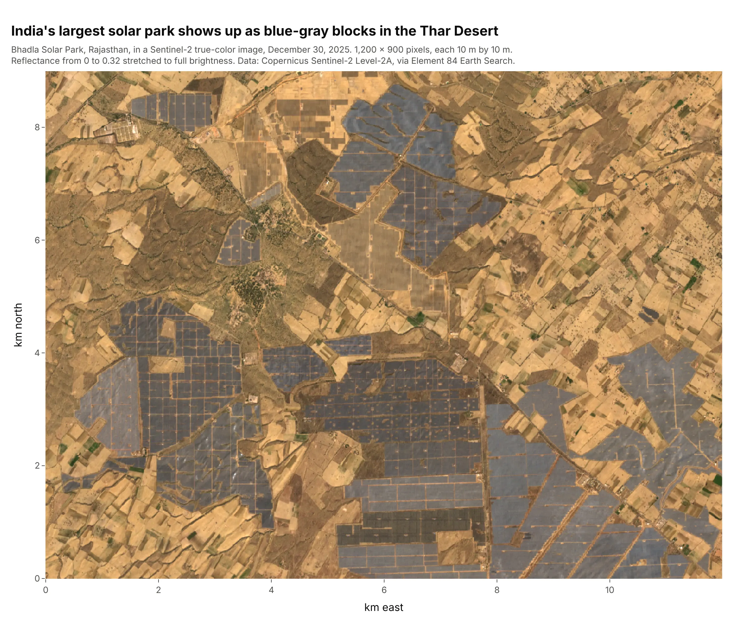
Data: Copernicus Sentinel-2 Level-2A image of December 30, 2025, via Element 84 Earth Search.

How do you read an image plot? In the example above, notice these things:

• Each pixel is one 10 m by 10 m square of ground, and the image has 1,200 columns and 900 rows of them. Because the axes are in kilometers and the pixels are drawn square, distances in the image are true distances.
• There's no color scale, because each pixel carries three numbers (the red, green and blue light the satellite measured), and their mix is the color you see. The blue-gray blocks are fields of solar panels, part of the 56 square kilometers (km²) of India's largest solar park, and the tan and brown patches around them are sand and farm fields.
• The brightness is a choice. The satellite stores reflectance (the share of sunlight bounced back), and here a reflectance of 0.32 is mapped to full brightness with zmax; without it the desert would look almost black.
• An image array starts at the top-left corner, with row 0 at the top. This one is drawn with origin="lower" and a y axis in kilometers north, so north is up and the numbers on the axis increase upward.

It's often used for charts like these:

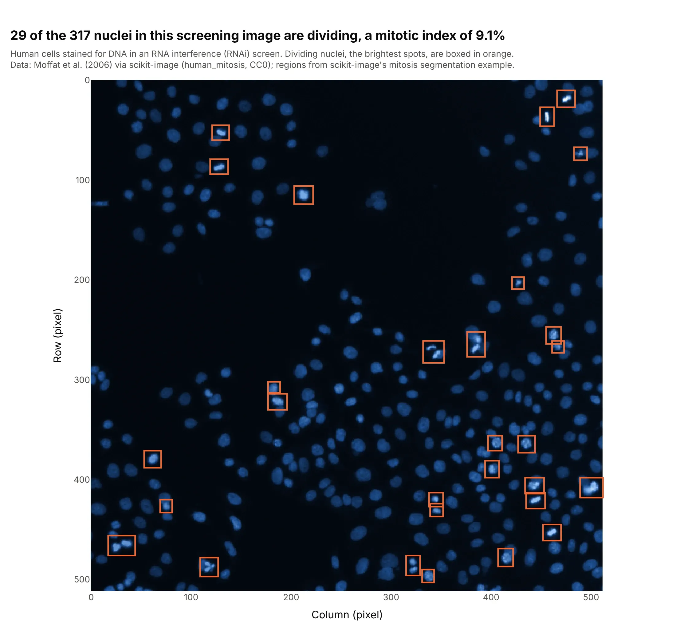
Microscopy. Drug screens image thousands of wells of cells, and this one from a genetic screen has 317 nuclei, 29 of them dividing (boxed), a mitotic index of 9.1%. Data: Moffat et al. (2006) via scikit-image (human_mitosis, CC0, a public domain dedication), with the regions from scikit-image's mitosis segmentation example.

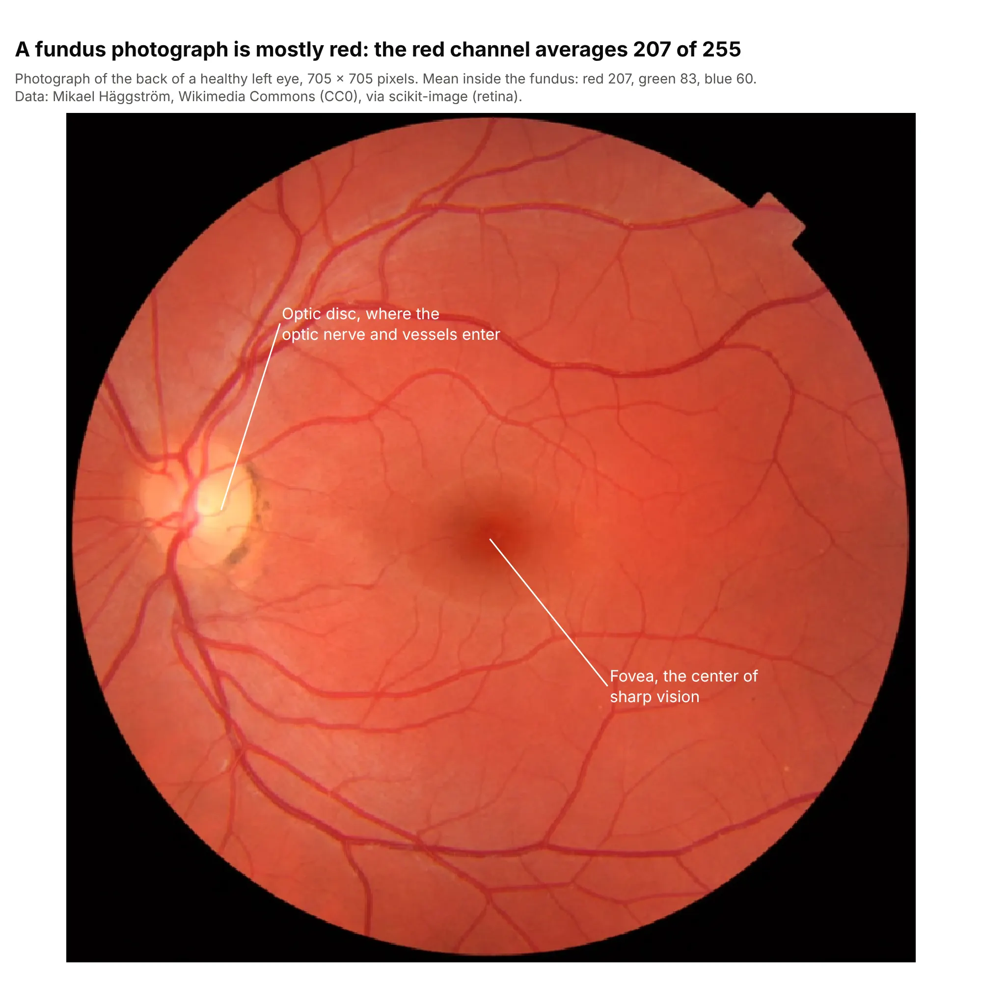
Medical imaging. A photograph of the retina is an RGB image, and annotations with leader lines point a reader to the optic disc and the fovea; the red channel averages 207 of 255. Data: Mikael Häggström, Wikimedia Commons (CC0), via scikit-image (retina).

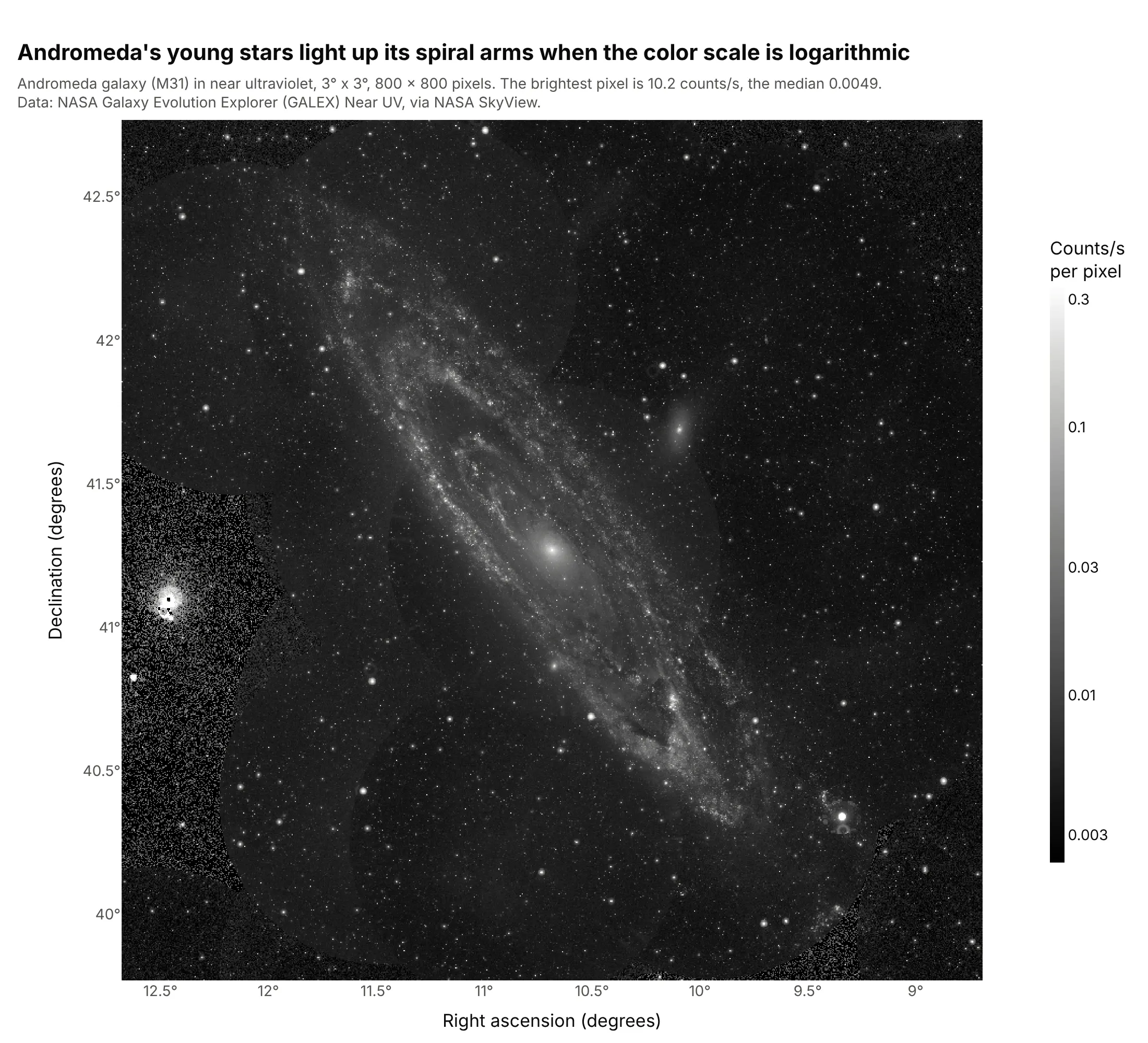
Astronomy. Telescope images span thousands of times in brightness, so they are drawn on a log scale: here the brightest pixel is 10.2 counts per second and the median 0.0049. Data: NASA Galaxy Evolution Explorer (GALEX) Near UV, via NASA SkyView.

How images become arrays

An image plot is easy to make and easy to get subtly wrong, because a few conventions sit between the numbers and the picture. These are the ones to know.

Pixels and channels

A digital image is a grid of numbers. A photograph has three numbers per pixel, one for each of red, green and blue (RGB), so in Python it's an array of shape (rows, columns, 3); a fourth channel, alpha, sets transparency. Most scientific images have one number per pixel instead, such as a temperature, an elevation or the light a microscope camera counted, so the array is (rows, columns). Ordinary photos store each channel as a whole number from 0 to 255 (8-bit, uint8), while cameras in labs and on satellites often use 0 to 65,535 (16-bit) or decimals.

Single-channel images need a color scale

With one number per pixel, px.imshow maps the values to colors with a color scale and draws a colorbar, exactly like a heatmap. Use a sequential scale (gray, or light to dark in one hue) for values with a natural low end, such as elevation or brightness, and a diverging scale with a midpoint for values that are positive or negative around a meaningful zero. With three channels, there's no color scale: the numbers are the colors.

Contrast: zmin and zmax

zmin and zmax set which values map to the darkest and lightest colors, and everything outside is clipped. By default px.imshow uses the data's minimum and maximum for a single-channel image, and the range of the data type (0 to 255 for 8-bit) for RGB. That's the right choice for elevation, but for an image with a few very bright pixels it makes everything else black. Here is the same Andromeda image three ways.

From the minimum to the maximum, the default, the brightest pixel (10.2) sets the top of the scale, and 99% of the pixels are below 0.039, so the image is almost black:

Clipped at the 1st and 99.5th percentiles, the galaxy and the stars appear, but the core and the brightest stars are saturated white:

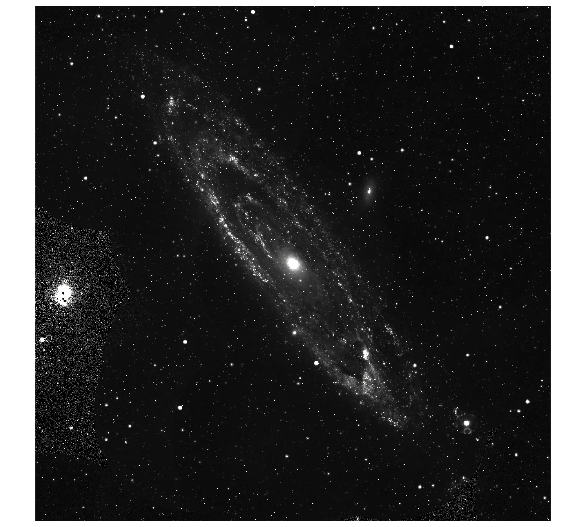
On a log scale, with np.log10 of the data and the limits at the 1st and 99.9th percentiles, the faint outer arms and the bright core both keep detail. Label the colorbar in the original units, as example 4 does:

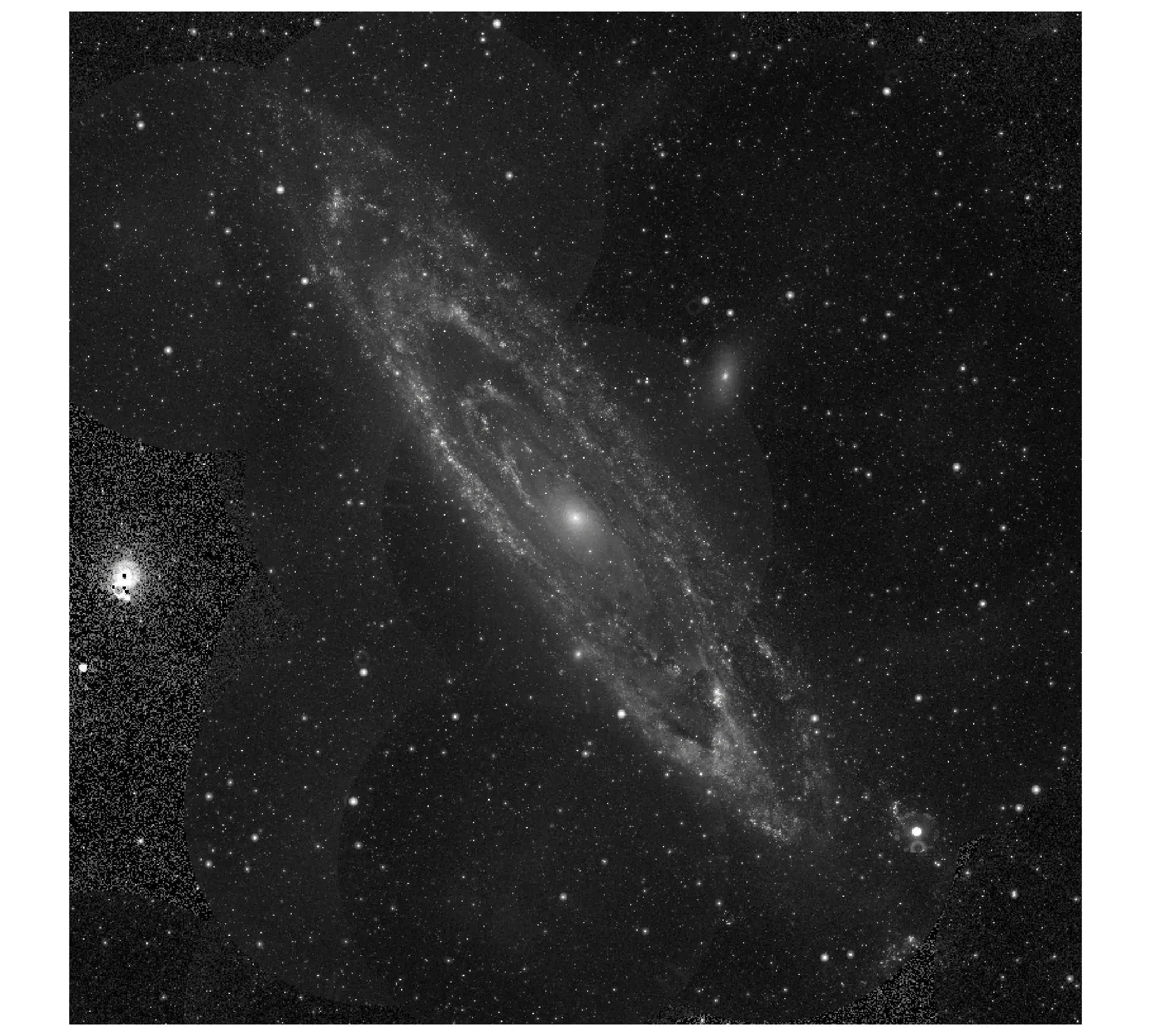
For RGB images, zmin and zmax take one value per channel (zmax=[3200, 3200, 3200]) or one for all three, which is how the solar park image maps a reflectance of 0.32 to full brightness. The contrast_rescaling="minmax" option does the minimum-to-maximum stretch per channel for you.

Origin, coordinates and aspect

An image array starts at the top-left corner, so px.imshow draws row 0 at the top with the y axis increasing downward (origin="upper"), the same as matplotlib's imshow. Two kinds of data break that convention. Gridded data from Network Common Data Form (NetCDF) files and many climate and ocean models store latitude increasing with the row, and astronomy's Flexible Image Transport System (FITS) files store the first row at the bottom; both need origin="lower". When you pass real coordinates as x and y, such as kilometers, latitudes or millimeters, px.imshow places each row and column at its coordinate, and origin="lower" gives the y axis that increases upward that those coordinates expect.

px.imshow also keeps pixels square by linking the two axes (scaleanchor), which is right when both axes share units. Set aspect="auto" to let the image fill the plot instead, which is fine for a matrix but distorts a photograph. When the units differ, set the ratio yourself: at 45° north a degree of longitude is about 71% as long as a degree of latitude, so the Europe example sets xaxis.scaleratio to cos(45°), and the MRI example passes coordinates in millimeters because its pixels are 1 mm wide and 1.33 mm tall.

Image plot or heatmap?

They are close relatives, and for a single-channel array px.imshow actually draws a heatmap trace. The difference is in the defaults and the intent. An image plot treats the array as a picture: square pixels, row 0 at the top, often hundreds of thousands of pixels, axes in pixels or physical units, and no gaps between cells. A heatmap usually shows a table, such as a correlation matrix or sales by weekday and hour, with category labels on the axes, cells that can be rectangles of any shape, and often the value printed in each cell. Use px.imshow for images and grids of measurements, and go.Heatmap or px.imshow(df, text_auto=True, aspect="auto") for labeled tables.

A short history

The first digital image was scanned in 1957 at the US National Bureau of Standards (now the National Institute of Standards and Technology), where Russell Kirsch fed a photograph of his three-month-old son into its Standards Eastern Automatic Computer (SEAC) as a grid 176 pixels on a side. John Hunter's matplotlib, first released in 2003 as a MATLAB-like plotting library (its name blends MATLAB, plot and library), gave Python the imshow and matshow functions most people still reach for (Hunter 2007). Plotly added an image trace to plotly.js in October 2019 and a "matplotlib-style" px.imshow to plotly.py a few weeks later, then binary_string in 2020, facet_col and animation_frame the same year, and facet_row in April 2026 (Plotly's changelog). We couldn't find Kirsch's original scan under a license we could reuse, so this guide doesn't redraw it.

Alternatives to an image plot

Here's the same grid of Mount Fuji elevations drawn six ways. Some are better for the question, some worse, some just different:

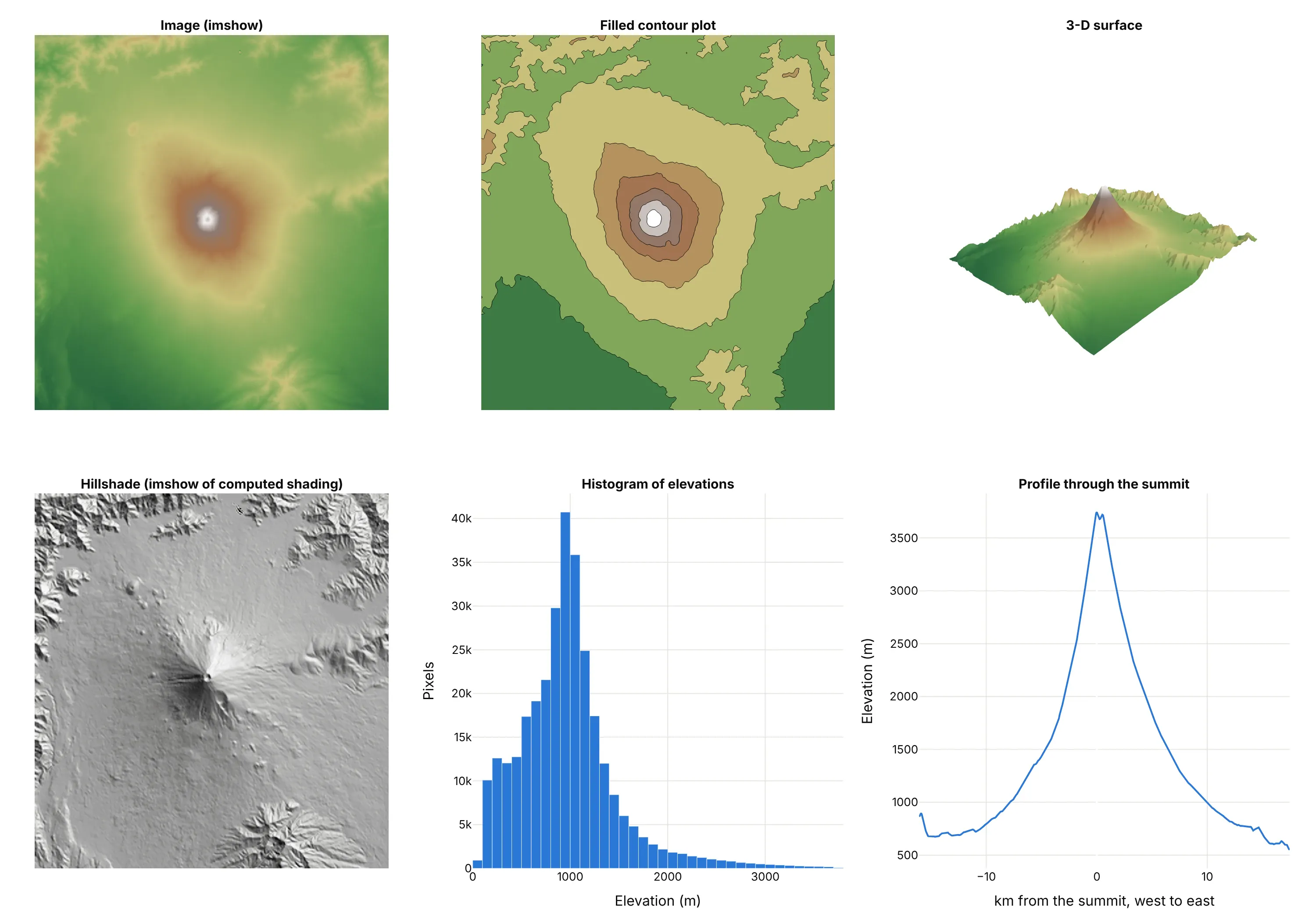
• Image plot (the default for a grid of measurements). Every pixel is shown with its value on hover, and it scales to millions of pixels.
• Contour plot (better for reading levels). Bands every 500 m make it easy to say which areas are above 2,000 m, but the detail inside each band is gone.
• 3-D surface (different, good for shape). It shows the cone at a glance and can be rotated, but values are hard to read off and the far side is hidden.
• Hillshade (works too, for terrain). It's still an image plot, of shading computed from the slopes, and shows ridges and valleys better than any color scale, but not the elevation itself.
• Histogram of pixel values (different). It shows how much of the area is at each elevation, and nothing about where. Use it to choose zmin and zmax.
• Line profile (better for one cross-section). A line chart along one row gives exact elevations along the way, which an image can't.

How to make an image plot

With AI

ChatGPT, Claude Code, GitHub Copilot, Cursor and other AI tools are excellent at writing Plotly code. Name Plotly in the prompt, and say whether the array is RGB or one channel, where the origin is, and how to set the contrast:

With Plotly Studio

Plotly Studio is a desktop app where you point an AI at a dataset and it builds charts and a Dash app around your questions. Ask for an image plot the same way:

Show the monthly NDVI images of these fields as an image plot with a slider through the months, a fixed color scale from 0 to 0.9 in browns and greens, and a line chart below of the share of pixels above 0.5 each month.

Make an image plot in Python or JavaScript

This is the code AI tools write under the hood. In Python, px.imshow takes a NumPy array, a PIL image, a pandas DataFrame or an xarray DataArray. An RGB image needs one line of code:

A single-channel array gets a color scale, and real coordinates go in x and y:

For more control, the two traces underneath are go.Image (for RGB, with z as an array or source as an image URL or base64 PNG) and go.Heatmap (for one channel). px.imshow sets up the square pixels and the reversed y axis for you, so with go.Heatmap add yaxis=dict(autorange="reversed", scaleanchor="x") to match it.

If you're coming from matplotlib, most arguments carry over: cmap becomes color_continuous_scale, vmin and vmax become zmin and zmax, origin and aspect work the same way, and extent becomes the x and y coordinate arrays. plt.matshow(m) is px.imshow(m).

In JavaScript, plotly.js draws a single-channel array as a heatmap trace with the y axis reversed and linked to x, which is what px.imshow does in Python:

For an RGB image, use {type: "image", source: "photo.png"} (an image URL or a base64 data URL) or {type: "image", z: rgbArray}; the image trace puts row 0 at the top and keeps pixels square on its own.

Share it

Every Plotly chart has a Share chart button (the cloud icon in its toolbar) that uploads it to Plotly Cloud and gives you a link. Only you can see it until you change its visibility.

For a live app, put the chart in a Dash app and publish it with the Plotly Cloud command-line interface (CLI). Coding agents can run these commands for you:

If your data has to stay in your own cloud or data center, publish to Dash Enterprise instead.

Dos and don'ts

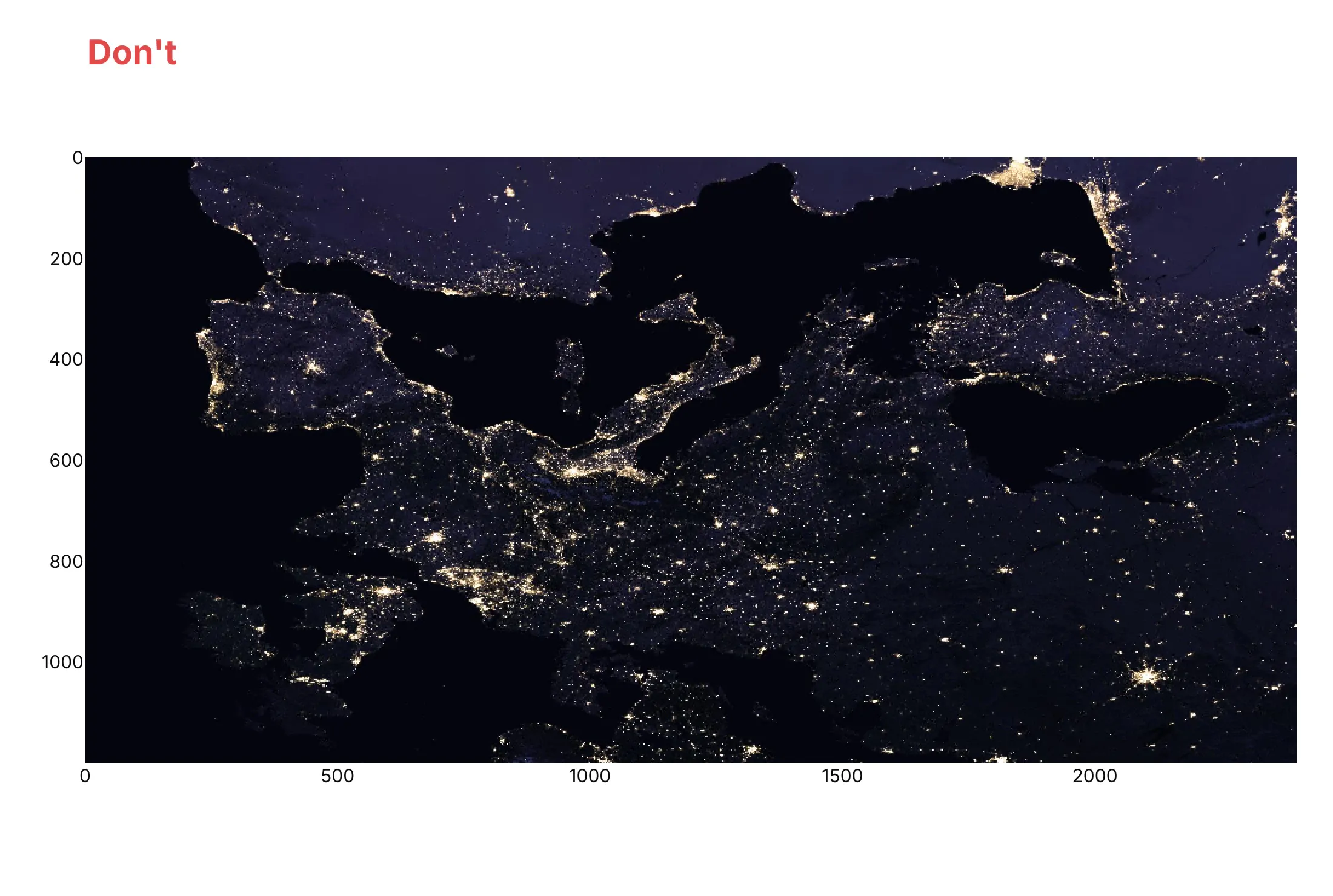
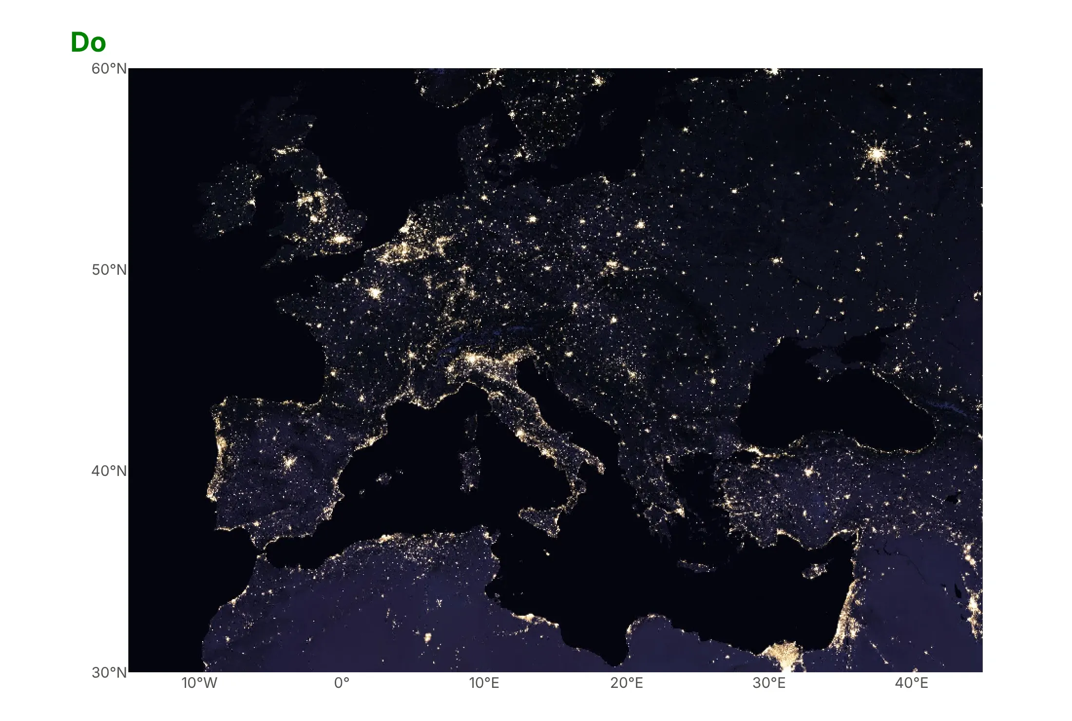
Most mistakes with image plots are about geometry rather than color: which way is up, whether pixels stay square, and what the axes mean. Here is Europe at night both ways, from the same array, whose rows run south to north as they do in many gridded files.

Don't pass the array with px.imshow's defaults, which puts its first row (the south) at the top and turns Europe upside down, set aspect="auto" so the image stretches to fill the box, or leave the axes in pixel numbers that mean nothing to a reader:

Do pass longitude and latitude as x and y with origin="lower", so north is up, keep the aspect equal with xaxis.scaleratio set to the cosine of the latitude, and label the axes in degrees:

Checklist

Do

• Check which way is up on an image you know, and set origin="lower" for gridded and FITS data.
• Pass physical coordinates (x, y) in kilometers, degrees, micrometers or millimeters, so hover and axes speak the reader's units.
• Set zmin and zmax deliberately, from percentiles or from the physical range, and use the same values across images you compare.
• Use a log scale for data that spans orders of magnitude, with the colorbar labeled in the original units.
• Use binary_string=True above about a million pixels, and binary_format="jpg" for photographs.
• Hide the axes on photographs where pixel numbers mean nothing.

Don't

• Stretch a photograph or map with aspect="auto"; keep pixels square or set the true ratio.
• Use a rainbow color scale such as jet for single-channel data; its bright bands invent edges that aren't in the data.
• Let each image in a stack pick its own color range when the reader compares them.
• Send a 16-megapixel float64 array as numbers to a browser; downsample it, send float32 or uint8, or use binary_string.

Options to customize

These are the options of px.imshow and the image and heatmap traces that matter most. The full lists are in the imshow documentation, the image trace reference and the heatmap trace reference.

1. zmin, zmax: the values mapped to the ends of the color scale; one number for a single channel, or a list per channel for RGB.
2. contrast_rescaling: "minmax" stretches each channel from its minimum to its maximum, "infer" uses the data type's range (0 to 255 for 8-bit).
3. color_continuous_scale, color_continuous_midpoint: the color scale for single-channel data, and the value at the middle of a diverging scale.
4. origin: "upper" (the default) puts row 0 at the top, "lower" at the bottom.
5. x, y: coordinates of the columns and rows, so axes and hover use physical units.
6. aspect: "equal" keeps pixels square, "auto" fills the plot area; xaxis.scaleratio sets any other ratio.
7. binary_string, binary_format, binary_compression_level: send the image as a PNG or JPEG string instead of numbers, for speed and file size; single-channel images then show in gray without a colorbar.
8. facet_col, facet_col_wrap, facet_row: split an axis of a 3-D or 4-D array into small multiples with linked zoom.
9. animation_frame: turn an axis of the array into frames with a slider and a play button.
10. labels: names for x, y and color in the hover and the colorbar.
11. text_auto: print each pixel's value, for small matrices only.
12. fig.add_shape(editable=True), layout.newshape and the drawrect, drawclosedpath, drawcircle and eraseshape modebar buttons: draw or let readers draw regions of interest (ROIs) on the image; in Dash, the shapes come back in relayoutData.
13. zsmooth: smooths between pixels instead of drawing hard-edged squares ("best" or "fast" on a heatmap, "fast" on an image trace).

More image plot examples

Six more image plots built from real public data, each with its source, the technique that makes it work and a prompt to rebuild it.

1. A year of center-pivot fields in Kansas, as an animation

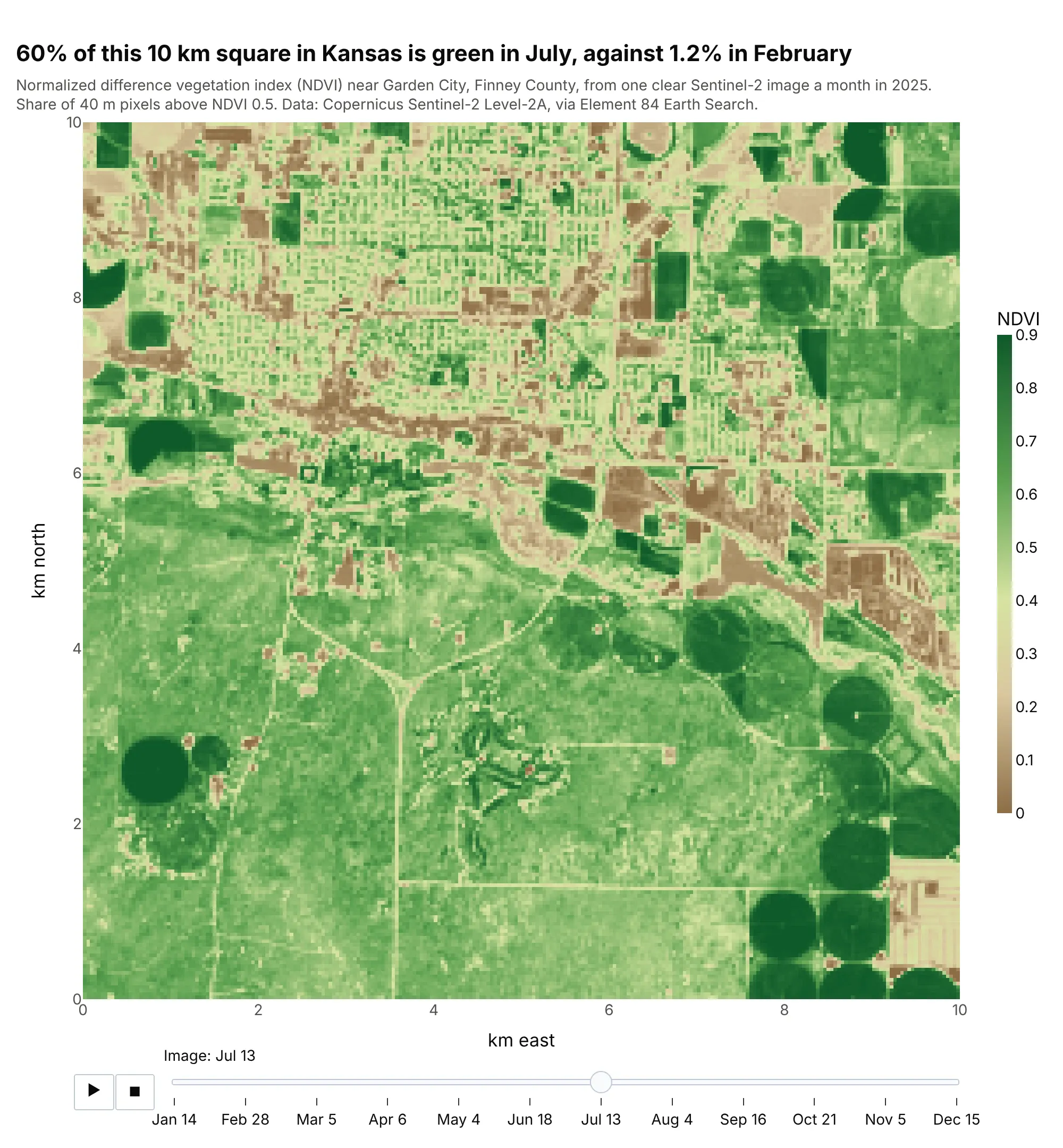
The normalized difference vegetation index (NDVI) measures how much of the ground is covered by green leaves, from about 0.1 for bare soil to 0.9 for a dense crop. Near Garden City, 60% of the area is above 0.5 in July and 1.2% in February, and the slider shows which circles of irrigated fields green up first. Data: Copernicus Sentinel-2 Level-2A, one clear image a month in 2025, via Element 84 Earth Search.

Tip: with animation_frame, fix zmin and zmax so a color means the same NDVI in every frame.

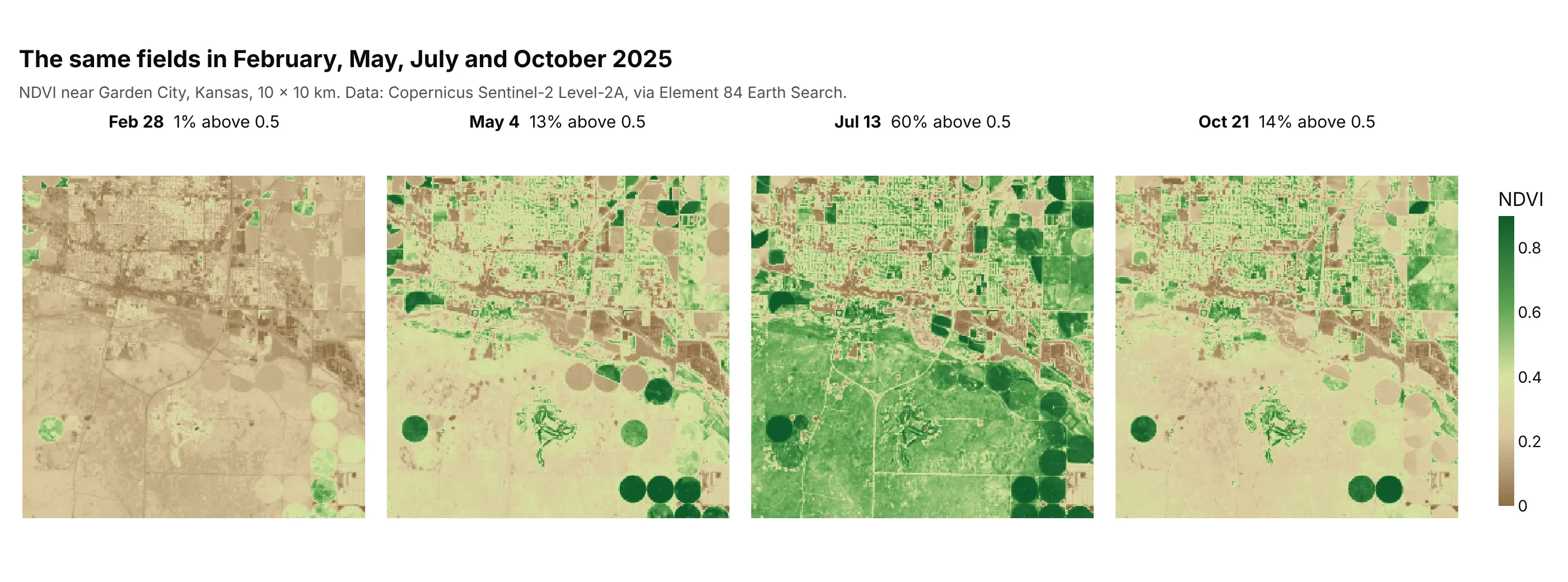
Another way to see it: small multiples with facet_col show four months at once, which is better on paper and in a slide, while the animation is better for finding the month a field changed:

2. Europe at night, 2.9 megapixels sent as a JPEG

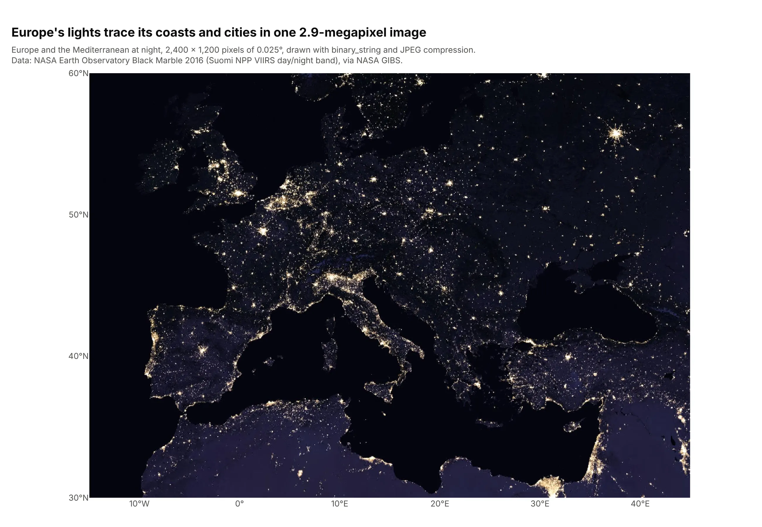
This composite of satellite images has 2.9 million pixels and 8.6 million RGB values. Sent as numbers, the figure's data takes 11.9 MB; with binary_string=True and binary_format="jpg" it takes 0.57 MB, so the page loads fast and the zoom stays smooth. Data: NASA Earth Observatory Black Marble 2016 (the day/night band of the Visible Infrared Imaging Radiometer Suite, VIIRS, on the Suomi NPP satellite), via NASA's Global Imagery Browse Services (GIBS).

Tip: use JPEG for photographs and PNG (the default) for images with sharp edges or exact values, such as masks and labels.

3. Mount Fuji's elevation with contour lines on top

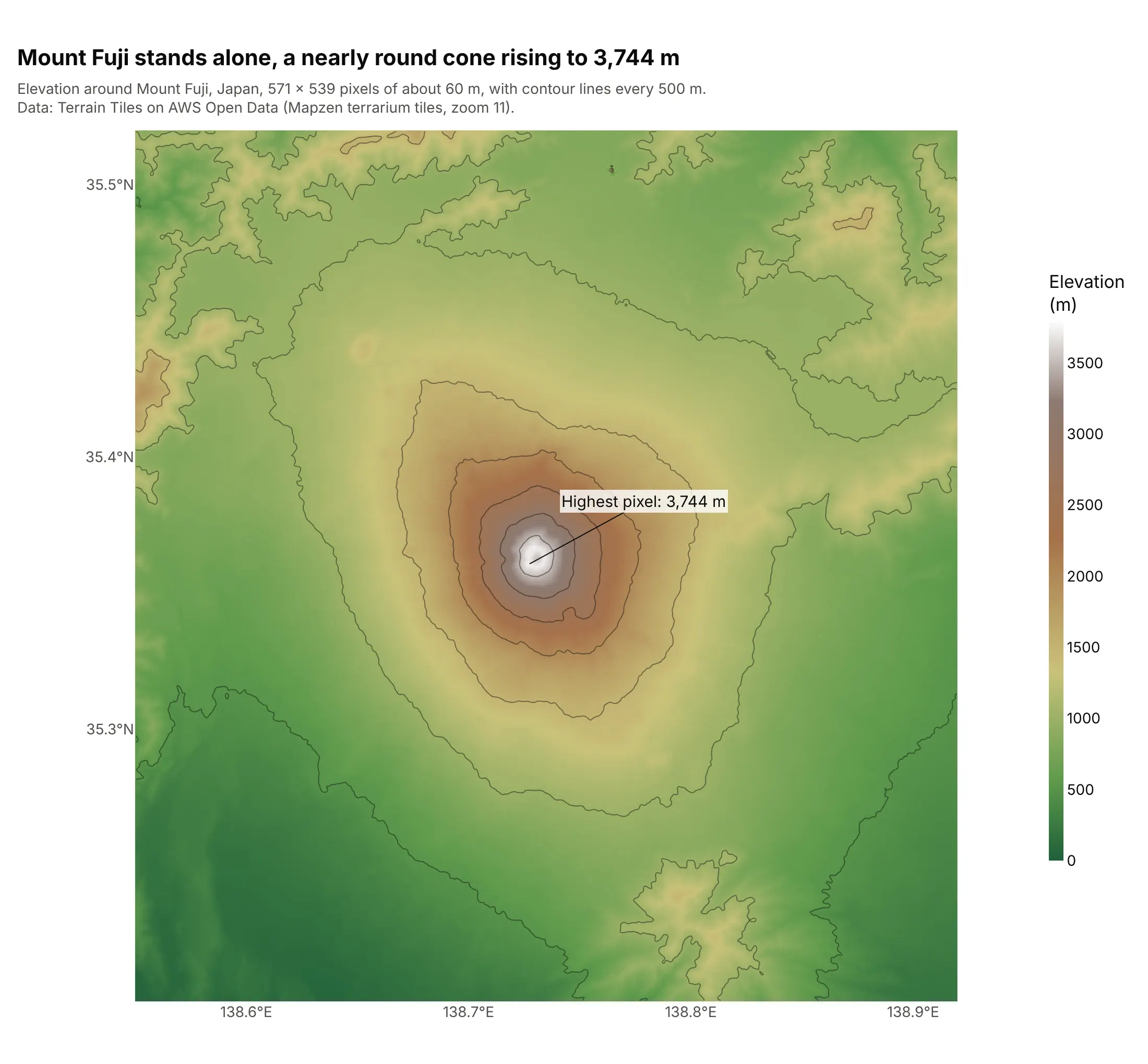
Each pixel is the average elevation of about 62 by 62 m of ground, so the highest pixel is 3,744 m, a little below the summit's official 3,776 m. The contour lines every 500 m form nearly round rings, which is the shape of a stratovolcano. Data: Terrain Tiles on AWS Open Data (Mapzen terrarium tiles, zoom 11).

Tip: overlay go.Contour with contours.coloring="none" on the same x, y and z to add contour lines without hiding the image.

4. Three fluorescence channels of mouse kidney tissue

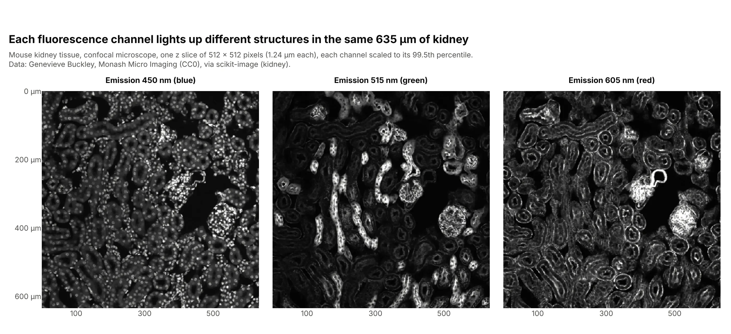
A confocal microscope records each fluorescent dye as a separate channel, and each one shows different structures in the same 635 micrometers (µm) of kidney: hundreds of small round spots at 450 nanometers (nm), a few bright filled tubes at 515 nm and the outlines of many others at 605 nm. Data: Genevieve Buckley, Monash Micro Imaging (CC0), via scikit-image (kidney).

Tip: facet_col=0 turns the first axis of a 3-D array into panels with linked zoom; scale each channel to its own percentile first, because the panels share one color axis.

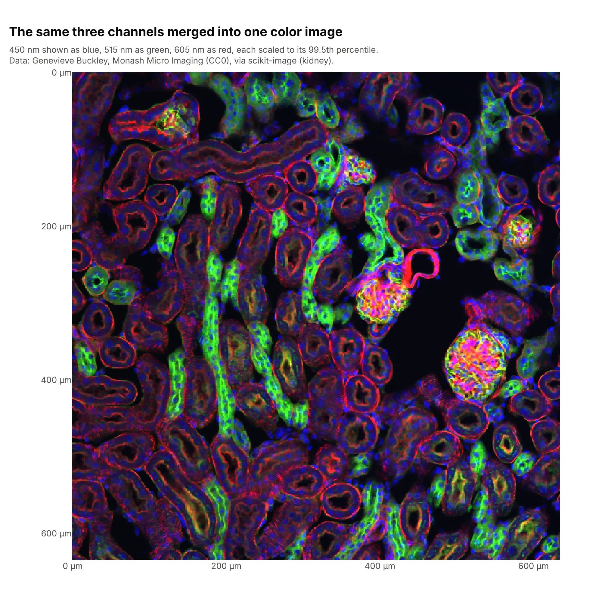
Another way to see it: merged into one RGB image, with each channel as one color, the three show how the structures sit together, while the panels show each one clearly:

5. A brain MRI scan as a grid of slices

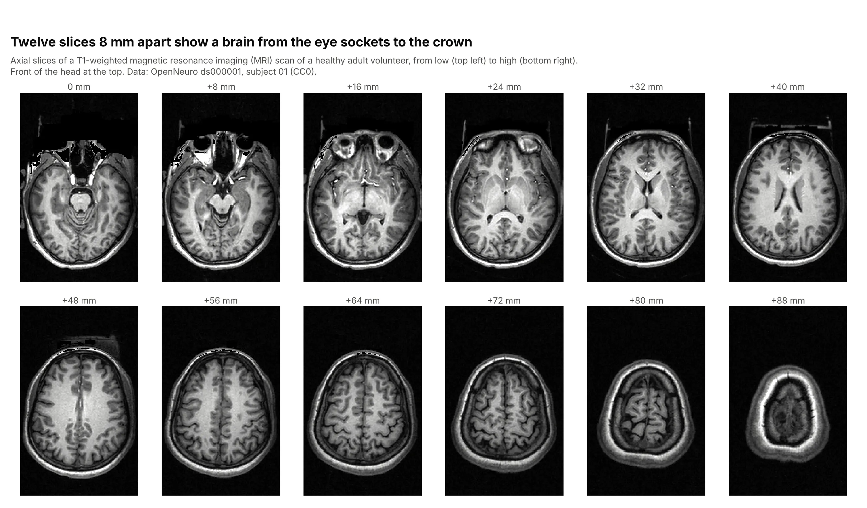
A magnetic resonance imaging (MRI) scan is a 3-D array, and twelve slices 8 mm apart show this healthy volunteer's brain from the eye sockets to the crown in one grid. The voxels are 1 mm wide and 1.33 mm front to back, so the coordinates are passed in millimeters to keep the head its true shape. Data: OpenNeuro ds000001, subject 01, T1-weighted (CC0).

Tip: for a whole volume, animation_frame=0 gives a slider through every slice, and facet_col_wrap a printable grid of a few.

6. The average handwritten digit, matshow style

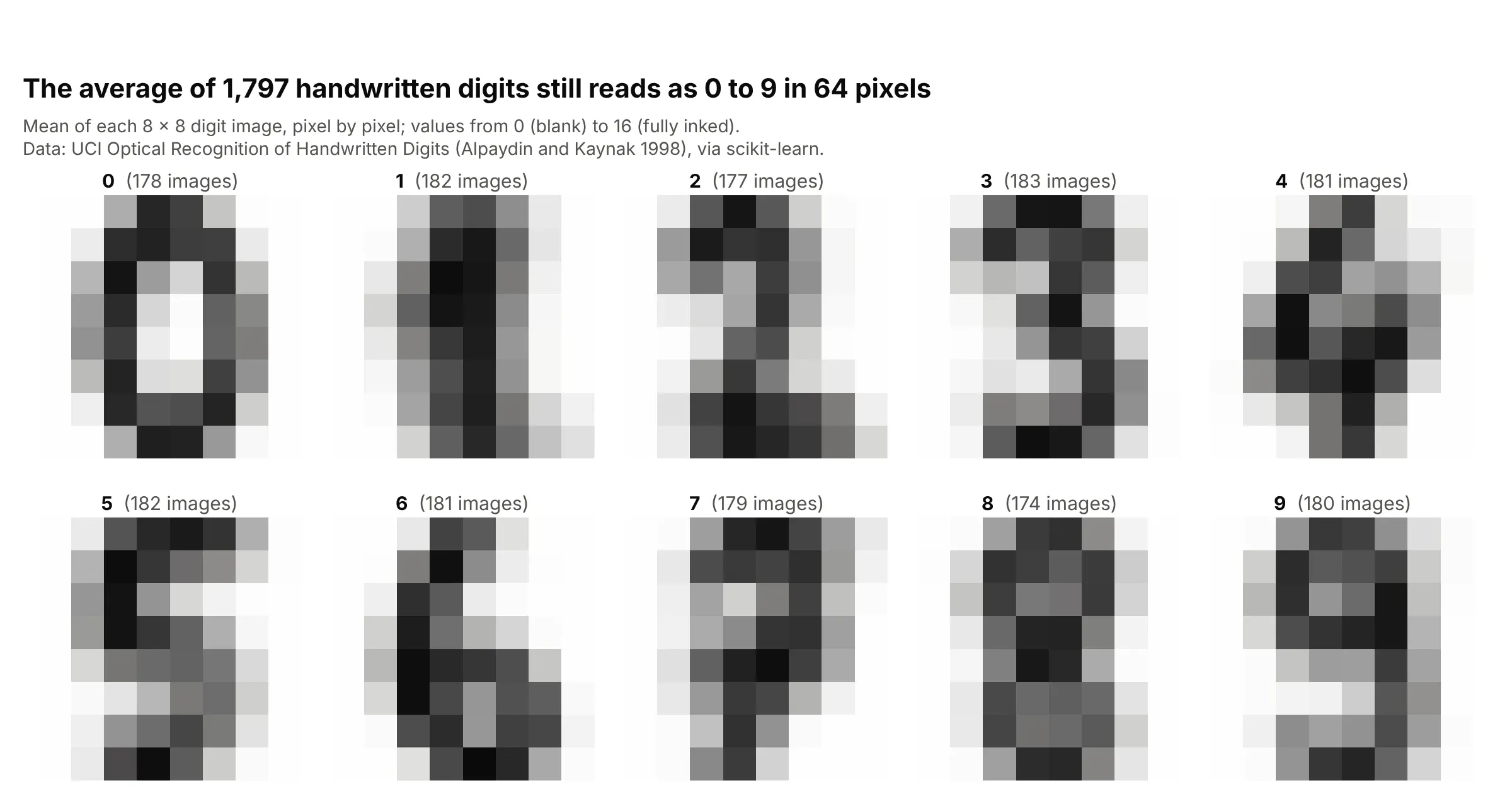
The 1,797 handwritten digits in this classic machine learning data set are 8 by 8 pixels, and averaging each digit pixel by pixel still gives a readable 0 to 9. This is what matplotlib's matshow is for: a small matrix shown as an image so its pattern shows at once. Data: University of California, Irvine (UCI) Optical Recognition of Handwritten Digits (Alpaydin and Kaynak 1998, CC BY 4.0), via scikit-learn's load_digits.

Tip: use a reversed gray scale ("gray_r") so ink is dark on white, as on paper.