Chris Parmer

November 4, 2026

Chord Diagrams - A Complete Guide

TL;DR

A chord diagram puts a set of groups around a circle and draws every flow or connection between two of them as a ribbon whose width is the size of the flow, so a whole origin-destination matrix fits in one picture.
Chord diagrams are also known as radial network diagrams, chord layouts and dependency wheels, and are similar to the Circos plots of genomics, Sankey diagrams and network graphs.
Use one for flows between 5 and about 20 groups that both send and receive, like migration between regions or trade between countries. For flows from one set of groups to another, use a Sankey; for exact values or many groups, a heatmap of the matrix.
You can make a chord diagram with Plotly from filled go.Scatter shapes: one arc per group and one ribbon per flow, made of two short arcs joined by Bezier curves through the center. This guide gives a reusable chord_diagram() helper in Python and the same chart in plotly.js.

What is a chord diagram?

Chord diagrams look like this:

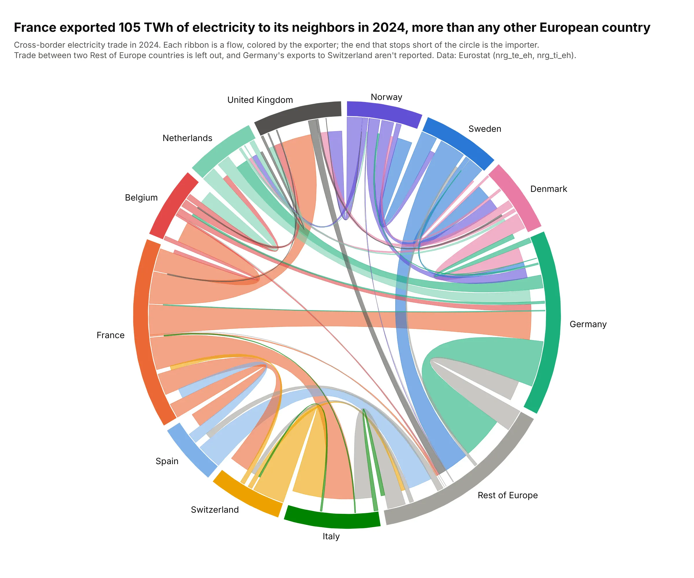
Chord diagram of electricity traded between European countries in 2024, with 11 countries and Rest of Europe around the circle in geographic order; France's orange arc is the longest and its ribbons run to Italy, the UK, Germany, Belgium, Switzerland and Spain, while Germany's green arc is mostly the ends of ribbons coming in

Data: Eurostat, electricity exports and imports by partner country (nrg_te_eh, nrg_ti_eh), 2024.

How do you read a chord diagram? In the example above, notice these things:

Each colored arc on the circle is one country, and its length is all the electricity it traded, exports plus imports. France's arc is the longest, at 120 TWh.
Each ribbon is the electricity one country sent to another, in the exporter's color, and its width at the circle is the size of the flow. The four widest are France to Italy, Switzerland to Italy, France to the UK and France to Germany, about 21 TWh each.
The end of a ribbon that stops short of the circle is the importer, which is how you tell the direction. Almost every orange ribbon ends short at another country, because France exported 105 TWh and imported 15.
A long arc doesn't mean a big exporter. Germany's arc is almost as long as France's, but most of it is the short ends of other countries' ribbons, since it imported 70 TWh and exported 47.
Watch what a chart leaves out. Rest of Europe groups 35 countries, so the trade among them isn't drawn, and Germany's exports to Switzerland are missing from the source data.

It's often used for charts like these:

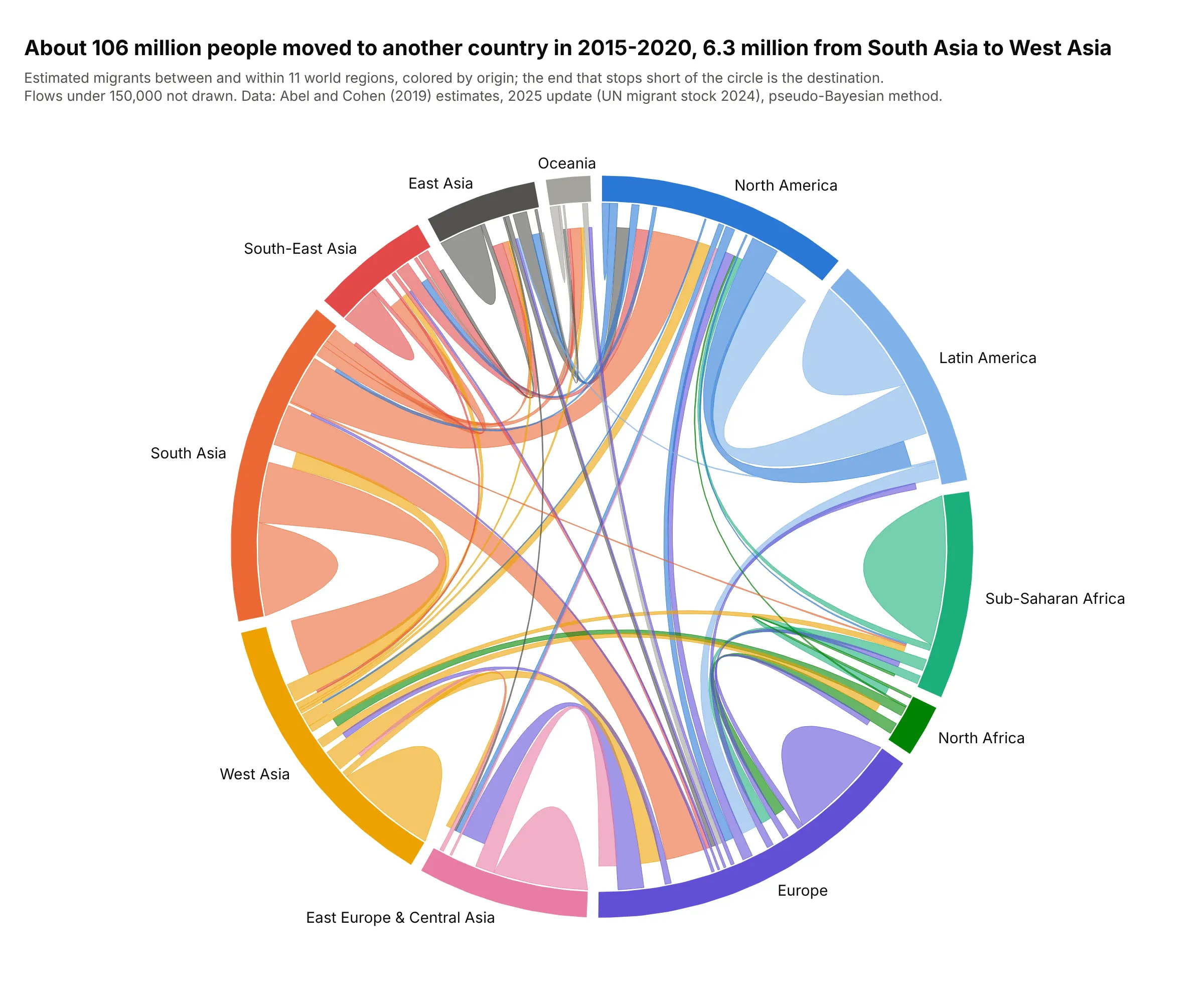
Chord diagram of an estimated 106 million people who moved to another country between 2015 and 2020, between and within 11 world regions; a wide orange ribbon runs from South Asia to West Asia and a wide light blue one from Latin America to North America, and loops show moves within Sub-Saharan Africa, Latin America and Europe

Migration between regions. An estimated 106 million people moved to another country from 2015 to 2020, and the largest flow between two regions was 6.3 million from South Asia to West Asia. Loops are moves between two countries in the same region. Data: Abel and Cohen (2019) estimates, 2025 update on figshare.

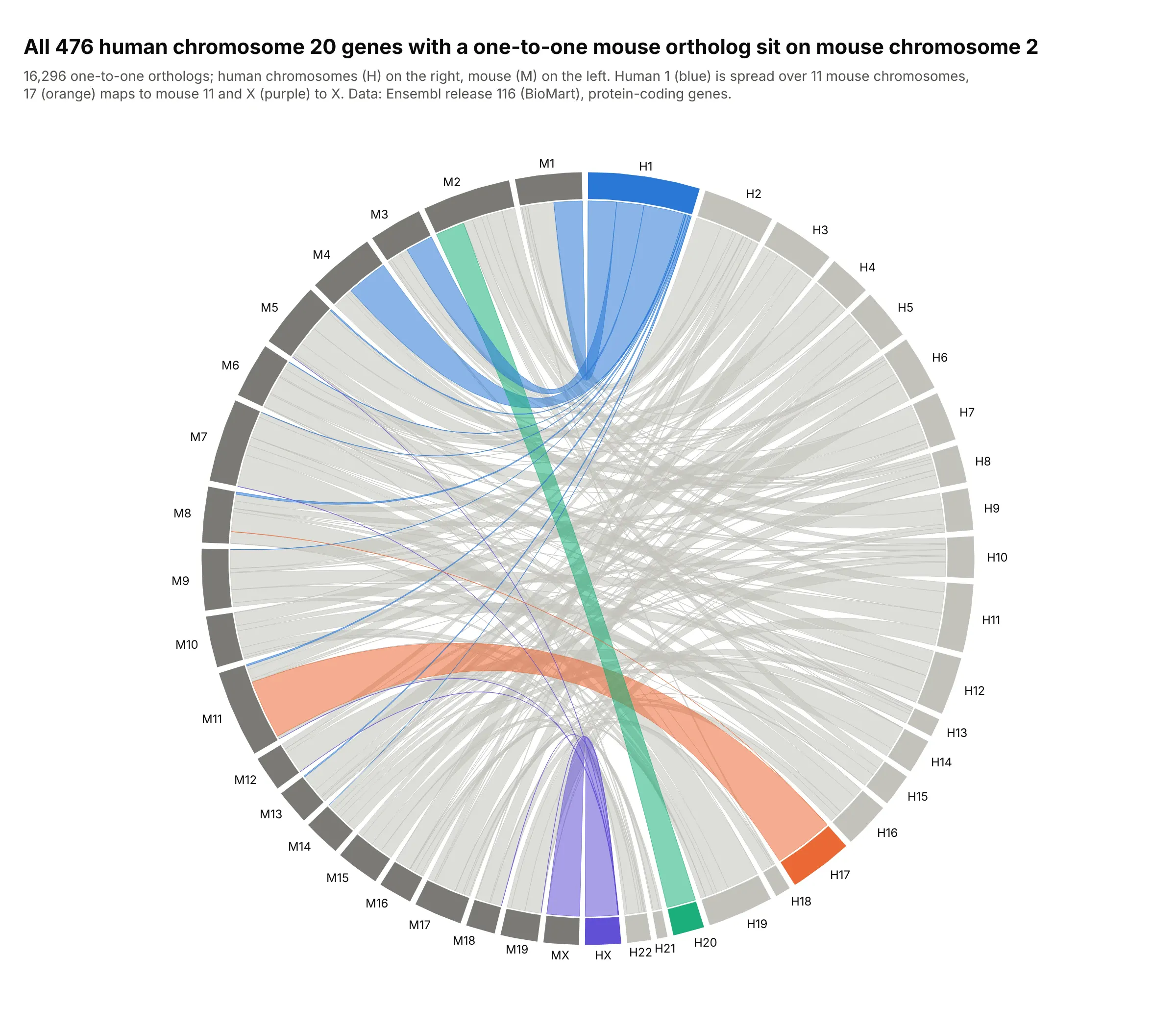
Circos-style chord diagram with human chromosomes on the right half and mouse chromosomes on the left, ribbons sized by shared one-to-one orthologous genes; human chromosome 20's green ribbon runs entirely to mouse chromosome 2, chromosome 17's orange ribbon to mouse 11, X to X, and chromosome 1's blue ribbons split over many mouse chromosomes

Comparative genomics. All 476 human chromosome 20 genes with a one-to-one mouse ortholog sit on mouse chromosome 2, while human chromosome 1's genes are spread over 11 mouse chromosomes. This two-sided layout is the Circos plot of genomics. Data: Ensembl release 116, BioMart.

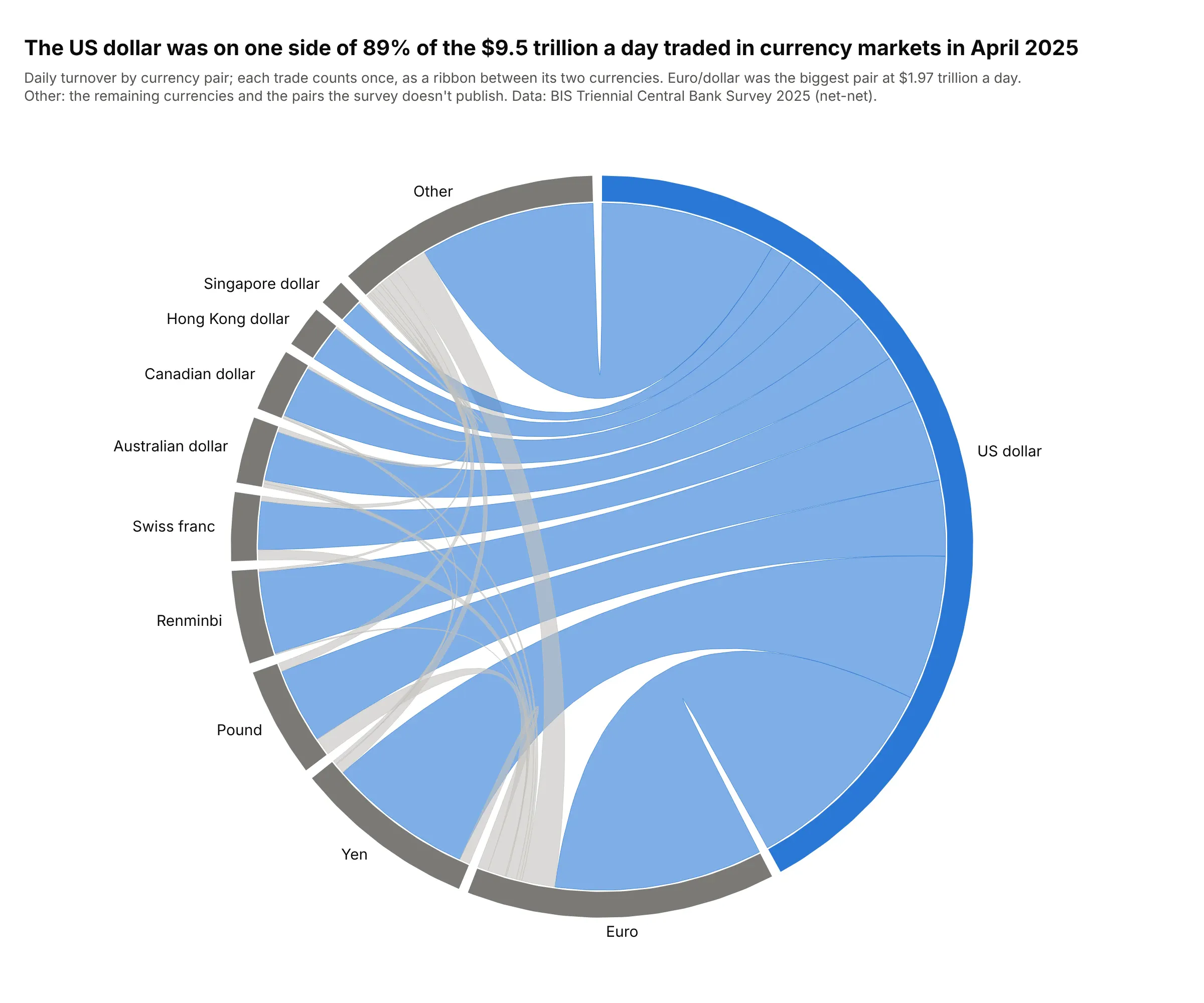
Chord diagram of currency trading by pair in April 2025: the US dollar's blue arc covers almost half the circle and blue ribbons run from it to the euro, yen, pound, renminbi and every other currency, while the few gray ribbons between other currencies are thin

Trade between markets. The US dollar was on one side of 89% of the $9.5 trillion a day traded in currency markets in April 2025, so almost every ribbon touches it. Each trade joins two currencies, so this chord diagram is undirected. Data: BIS Triennial Central Bank Survey 2025.

A short history

The circular layout with ribbons became widely known through genomics. Martin Krzywinski's Circos (Genome Research, 2009) put chromosomes around a circle and used "ribbons, which encode the position, size, and orientation of related genomic elements". D3's d3-chord, which brought chord diagrams to the web, still uses a matrix from the Circos documentation as its example. Abel and Sander (2014) then used one in Science to show global migration, estimating "the largest movements to occur between South and West Asia, from Latin to North America, and within Africa". This is their kind of chart redrawn with Plotly, from the same estimation method run on updated UN data:

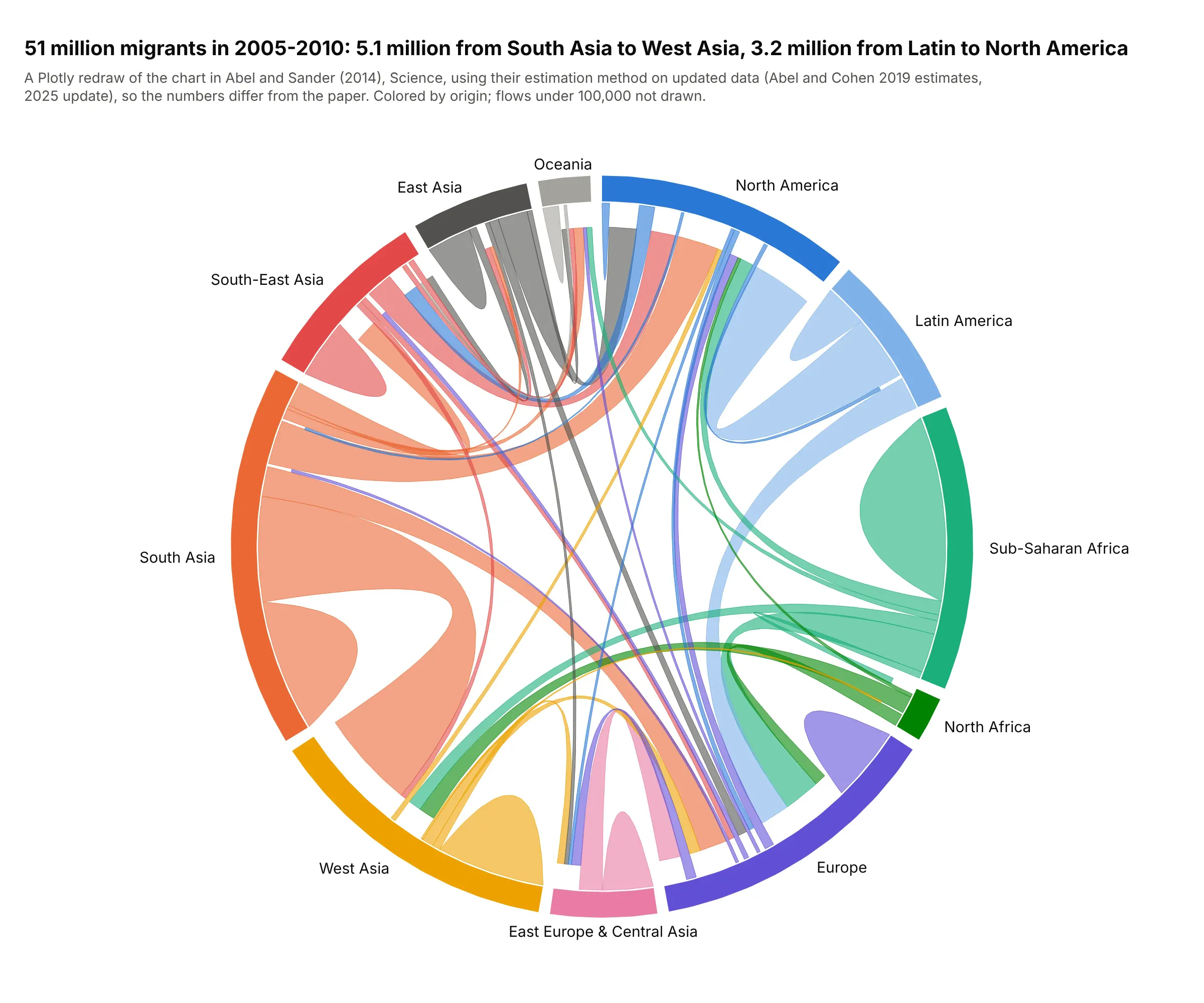
A redraw of Abel and Sander's 2014 chord diagram of global migration flows in 2005-2010: 51 million migrants between and within 11 regions, with the widest ribbons from South Asia to West Asia (5.1 million) and Latin America to North America (3.2 million), and a large loop within Sub-Saharan Africa

Data: Abel and Cohen (2019) estimates, 2025 update, closed demographic accounting with the minimisation method of Abel and Sander. The numbers differ from the paper's because the UN data have been revised.

Directed and undirected chord diagrams

A chord diagram draws a square matrix, and what the matrix holds decides how to read the ribbons.

Directed (migration, trade, electricity flows): the cell for A to B differs from B to A. Each group's arc is its outflow plus its inflow, A to B and B to A are two ribbons, and the chart has to show direction. Common ways are coloring by origin, leaving a gap at the destination end, as in this guide, or drawing an arrowhead.
Undirected (trading pairs, co-occurrence, shared genes): A with B is one number. Each pair gets one ribbon with both ends on the circle, and each arc is that group's row total. When one item can join several groups, like a trial with sites on three continents, the arcs add up to more than the number of items.
Within-group flows sit on the diagonal of the matrix, such as people moving between two European countries. Draw them as loops, as in the migration examples, or leave them out and say so.

Alternatives to a chord diagram

Here's the same European electricity trade drawn four ways. Some are better for the question, some worse, some just different:

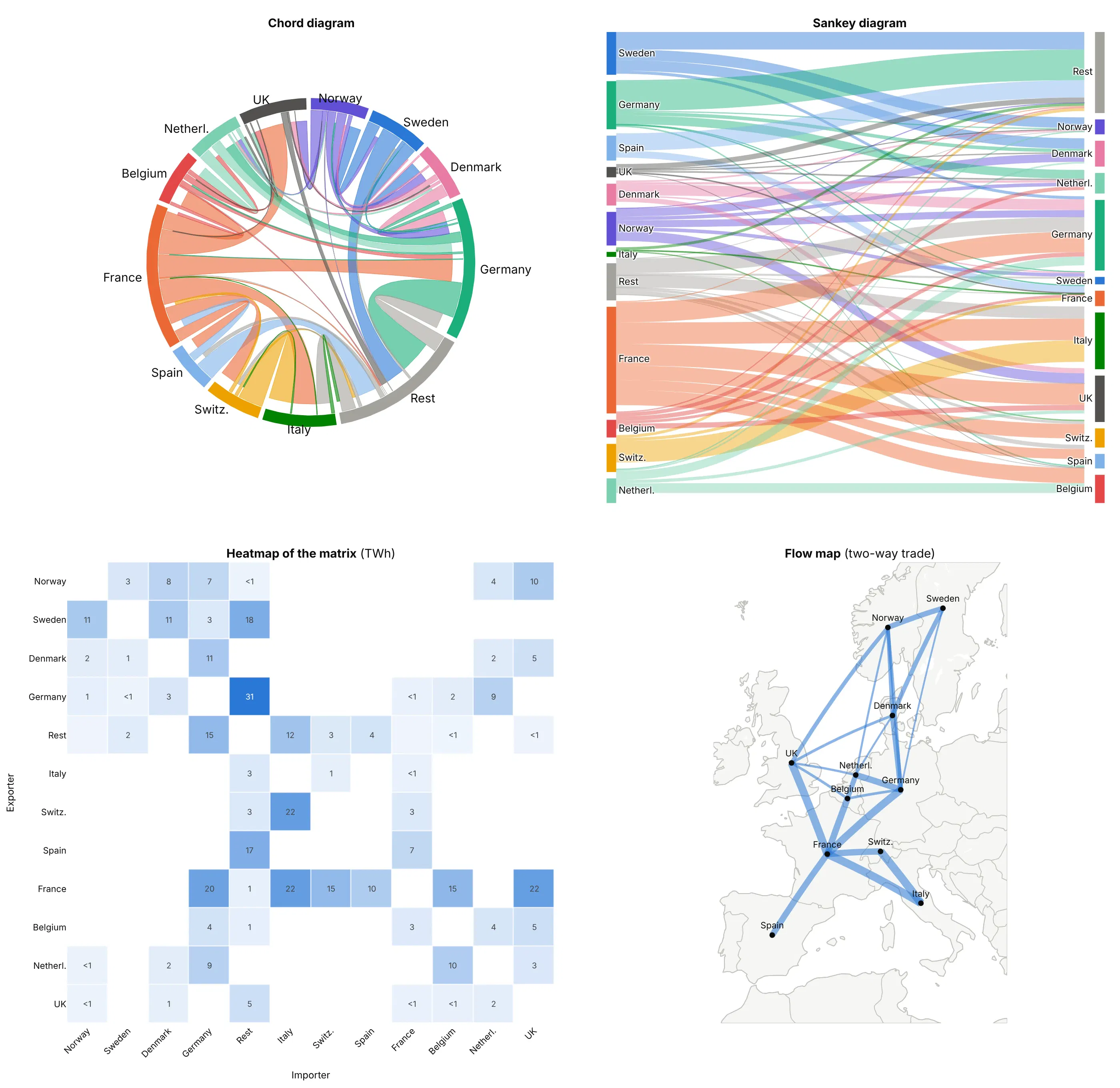
The 2024 European electricity trade drawn four ways: the chord diagram; a Sankey diagram with exporters on the left and importers on the right and many crossing links; a heatmap of the exporter by importer matrix with values in TWh, where France's row has the darkest cells; and a flow map of Europe with lines between country centers, thickest from France to Italy, the UK and Germany

Sankey diagram (better when sources and targets are different groups). Exporters on one side and importers on the other is easy to read when they're different sets, like fuels flowing to sectors. Here every country is on both sides, so the links cross and you can't see that France's exports and imports belong to one country.
Heatmap of the matrix (better for exact values). Every flow is a cell with its number, nothing hides behind another ribbon, and it works for 50 groups, but the totals and the overall pattern take longer to see.
Flow map (better when geography matters). Lines between places show that the trade runs between neighbors, which the circle loses, but it needs a location for every group, so Rest of Europe can't go on it, and the two directions merge.
Network graph (different). Nodes and edges suit many groups with few, unweighted links, like a citation network. With weighted flows between a dozen groups, the chord diagram's ribbon widths compare better.

How to make a chord diagram

With AI

ChatGPT, Claude Code, GitHub Copilot, Cursor and other AI tools are excellent at writing Plotly code. Name Plotly in the prompt, and say how the ribbons should be built and how direction should show:

Make a plotly chord diagram from electricity_trade.csv (columns: exporter, importer, twh).

- Pivot to a square matrix, rows = exporters, columns = importers, countries in geographic order.
- Draw each country as an arc around a circle (a filled go.Scatter annular sector) whose length is
  exports + imports, with a 2-degree gap between countries.
- Draw each flow as a filled go.Scatter ribbon: two short arcs joined by quadratic Bezier curves through
  the center, as wide as the flow at both ends, in the exporter's color at 0.6 opacity, with the
  importer's end stopping a little short of the circle.
- Hover text "France → Italy: 21.9 TWh", country labels outside the circle, hidden axes with
  scaleanchor so the circle stays round.
- Check: print each country's exports and imports and the five largest flows.

With Plotly Studio

Plotly Studio is a desktop app where you point an AI at a dataset and it builds charts and a Dash app around your questions. Ask for a chord diagram the same way:

Show a chord diagram of migration between world regions, ribbons colored by origin region with the destination end stopping short of the circle, regions in geographic order, and a dropdown to pick the five-year period.

Make a chord diagram in Python or JavaScript

This is the code AI tools write under the hood. You can make a chord diagram with Plotly from filled go.Scatter traces, so you get hover text, zoom and Dash callbacks like any other Plotly chart. This helper takes a matrix and returns a go.Figure; the version used for the images in this guide adds undirected mode, loops for within-group flows and a fixed scale for comparing two diagrams:

import numpy as np
import pandas as pd
import plotly.graph_objects as go

def chord_diagram(matrix, labels, colors, gap=2.0, unit=""):
    """matrix[i][j] = flow from labels[i] to labels[j]. Returns a go.Figure."""
    m = np.asarray(matrix, dtype=float)
    n = len(labels)
    xy = lambda deg, r: (r * np.sin(np.radians(deg)), r * np.cos(np.radians(deg)))  # clockwise from 12 o'clock
    arc = lambda a0, a1, r: xy(np.linspace(a0, a1, 30), r)
    scale = (360 - gap * n) / (m.sum(axis=0) + m.sum(axis=1)).sum()

    # each group's arc holds its exports to, then imports from, every partner, nearest neighbors at the edges
    slot, span, angle = {}, [], 0.0
    for i in range(n):
        start = angle
        for j in [(i - k) % n for k in range(1, n)]:
            for key, v in (((i, j, "out"), m[i, j]), ((i, j, "in"), m[j, i])):
                slot[key] = (angle, angle + v * scale)
                angle += v * scale
        span.append((start, angle))
        angle += gap

    fig = go.Figure()
    t = np.linspace(0, 1, 40)
    for i, j in sorted(np.argwhere(m > 0).tolist(), key=lambda p: -m[p[0], p[1]]):
        (s0, s1), (t0, t1) = slot[(i, j, "out")], slot[(j, i, "in")]
        p1, p2 = np.array(xy(s1, 1)), np.array(xy(t0, 0.93))  # the importer's end stops short of the circle
        p3, p4 = np.array(xy(t1, 0.93)), np.array(xy(s0, 1))
        bez = lambda a, b: ((1 - t) ** 2 * a[0] + t ** 2 * b[0], (1 - t) ** 2 * a[1] + t ** 2 * b[1])  # via center
        parts = [arc(s0, s1, 1), bez(p1, p2), arc(t0, t1, 0.93), bez(p3, p4)]
        fig.add_trace(go.Scatter(x=np.concatenate([p[0] for p in parts]), y=np.concatenate([p[1] for p in parts]),
                                 fill="toself", mode="lines", line_width=0, fillcolor=colors[i], opacity=0.6,
                                 hoveron="fills", hoverinfo="text", text=f"{labels[i]} → {labels[j]}: {m[i, j]:,.1f} {unit}"))
    for i, (a0, a1) in enumerate(span):
        (xo, yo), (xi, yi) = arc(a0, a1, 1.08), arc(a1, a0, 1.0)
        fig.add_trace(go.Scatter(x=np.r_[xo, xi], y=np.r_[yo, yi], fill="toself", mode="lines", line_width=0,
                                 fillcolor=colors[i], hoverinfo="skip"))
        lx, ly = xy((a0 + a1) / 2, 1.15)
        fig.add_annotation(x=lx, y=ly, text=labels[i], showarrow=False, xanchor="left" if lx > 0.1 else
                           "right" if lx < -0.1 else "center")
    fig.update_xaxes(visible=False, range=[-1.6, 1.6])
    fig.update_yaxes(visible=False, range=[-1.3, 1.3], scaleanchor="x")
    fig.update_layout(showlegend=False, plot_bgcolor="white", width=800, height=650)
    return fig

df = pd.read_csv("europe_electricity.csv")  # exporter_name, importer_name, gwh
countries = ["France", "Germany", "Austria", "Italy", "Switzerland"]
flows = df[df.exporter_name.isin(countries) & df.importer_name.isin(countries)]
matrix = flows.pivot_table(index="exporter_name", columns="importer_name", values="gwh", aggfunc="sum")
matrix = matrix.reindex(index=countries, columns=countries).fillna(0) / 1000  # TWh
fig = chord_diagram(matrix.values, countries, ["#eb6834", "#1baf7a", "#e34948", "#008300", "#eda100"], unit="TWh")
fig.show()

Ordering each group's partners from its nearest neighbor on one side round to its nearest neighbor on the other keeps ribbons from twisting across each other inside an arc. Drawing the widest ribbons first puts the thin ones on top, where you can still hover them. If your flows go from one set of groups to a different set, go.Sankey draws them with no helper at all.

In JavaScript, plotly.js draws the same thing from scatter traces with fill: "toself":

<div id="chart"></div>
<script src="https://cdn.plot.ly/plotly-4.1.1.min.js"></script>
<script>
  // Electricity trade in 2024, TWh, row = exporter, column = importer (Eurostat nrg_te_eh / nrg_ti_eh)
  const labels = ["France", "Germany", "Austria", "Italy", "Switzerland"];
  const colors = ["#eb6834", "#1baf7a", "#e34948", "#008300", "#eda100"];
  const m = [[0, 20.5, 0, 21.9, 14.7], [0.7, 0, 8.9, 0, 0], [0, 8.5, 0, 1.6, 2.9],
             [0.8, 0, 0.2, 0, 1.3], [3.1, 0, 2.7, 21.7, 0]];
  const n = labels.length, gap = 2;
  const xy = (deg, r) => [r * Math.sin(deg * Math.PI / 180), r * Math.cos(deg * Math.PI / 180)];
  const arc = (a0, a1, r) => Array.from({length: 30}, (_, k) => xy(a0 + (a1 - a0) * k / 29, r));
  const curve = (p, q) => Array.from({length: 40}, (_, k) => {    // quadratic Bezier through the center
    const t = k / 39; return [(1 - t) ** 2 * p[0] + t ** 2 * q[0], (1 - t) ** 2 * p[1] + t ** 2 * q[1]];
  });
  let total = 0; m.forEach((row, i) => row.forEach((v, j) => total += 2 * v));
  const scale = (360 - gap * n) / total;

  const slot = {}, span = []; let angle = 0;            // each arc: exports to, then imports from, each partner
  for (let i = 0; i < n; i++) {
    const start = angle;
    for (let k = 1; k < n; k++) {
      const j = (i - k + n) % n;
      slot[`${i}-${j}-out`] = [angle, angle += m[i][j] * scale];
      slot[`${i}-${j}-in`] = [angle, angle += m[j][i] * scale];
    }
    span.push([start, angle]); angle += gap;
  }

  const traces = [];
  for (let i = 0; i < n; i++) for (let j = 0; j < n; j++) {
    if (!m[i][j]) continue;
    const [s0, s1] = slot[`${i}-${j}-out`], [t0, t1] = slot[`${j}-${i}-in`];
    const pts = [...arc(s0, s1, 1), ...curve(xy(s1, 1), xy(t0, 0.93)), ...arc(t0, t1, 0.93),
                 ...curve(xy(t1, 0.93), xy(s0, 1))];       // the importer's end stops short of the circle
    traces.push({x: pts.map(p => p[0]), y: pts.map(p => p[1]), fill: "toself", mode: "lines", line: {width: 0},
                 fillcolor: colors[i], opacity: 0.6, hoveron: "fills", hoverinfo: "text",
                 text: `${labels[i]} → ${labels[j]}: ${m[i][j]} TWh`});
  }
  const annotations = span.map(([a0, a1], i) => {
    const pts = [...arc(a0, a1, 1.08), ...arc(a1, a0, 1)];
    traces.push({x: pts.map(p => p[0]), y: pts.map(p => p[1]), fill: "toself", mode: "lines", line: {width: 0},
                 fillcolor: colors[i], hoverinfo: "skip"});
    const [x, y] = xy((a0 + a1) / 2, 1.15);
    return {x, y, text: labels[i], showarrow: false, xanchor: x > 0.1 ? "left" : x < -0.1 ? "right" : "center"};
  });

  Plotly.newPlot("chart", traces, {
    width: 800, height: 650, showlegend: false, annotations, plot_bgcolor: "white",
    xaxis: {visible: false, range: [-1.6, 1.6]}, yaxis: {visible: false, range: [-1.3, 1.3], scaleanchor: "x"}
  });
</script>

Share it

Every Plotly chart has a Share chart button (the cloud icon in its toolbar) that uploads it to Plotly Cloud and gives you a link. Only you can see it until you change its visibility.

For a live app, put the chart in a Dash app and publish it with the Plotly Cloud CLI. Coding agents can run these commands for you:

pip install "dash[cloud]"
plotly user login
plotly app publish

If your data has to stay in your own cloud or data center, publish to Dash Enterprise instead.

Dos and don'ts

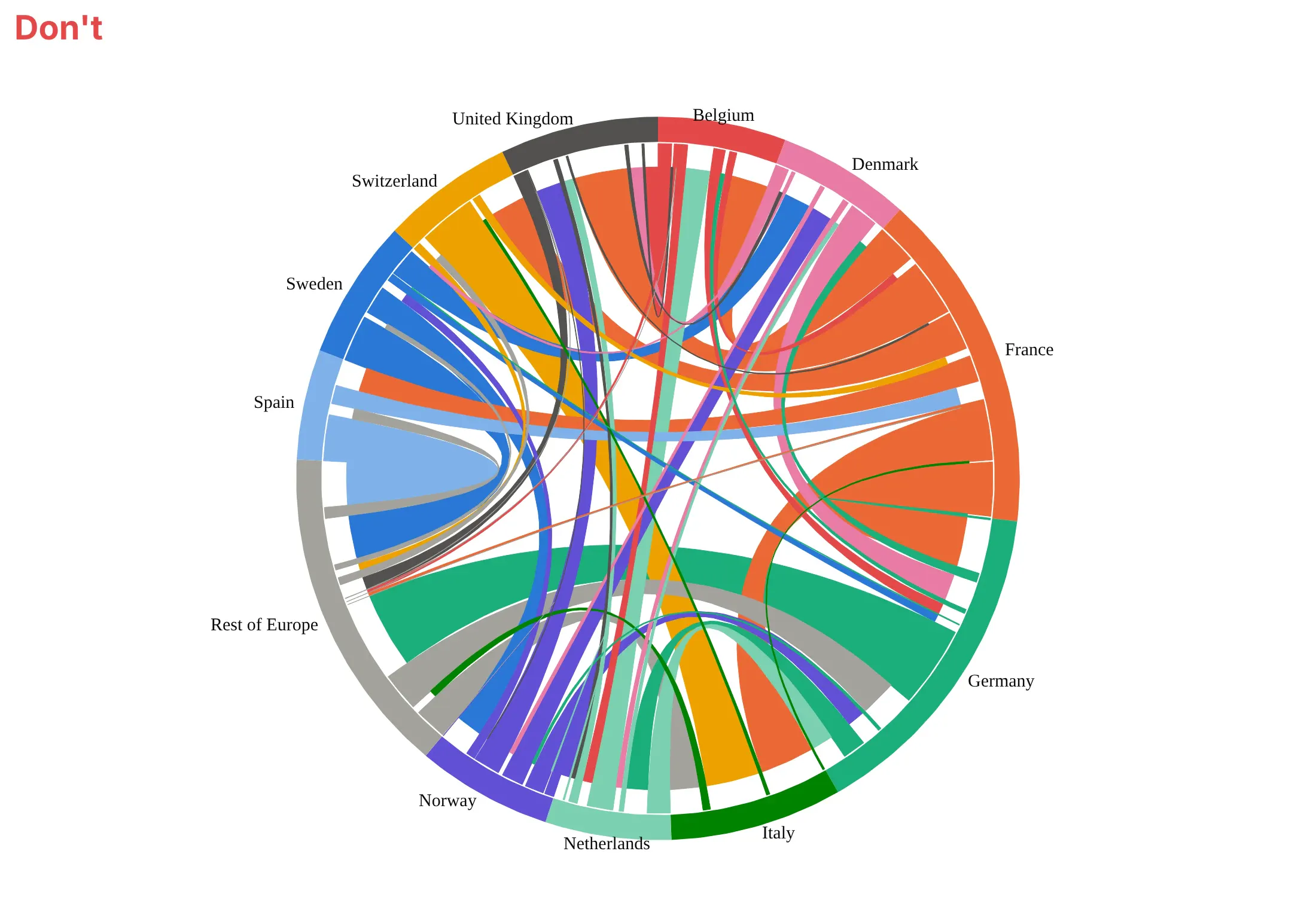
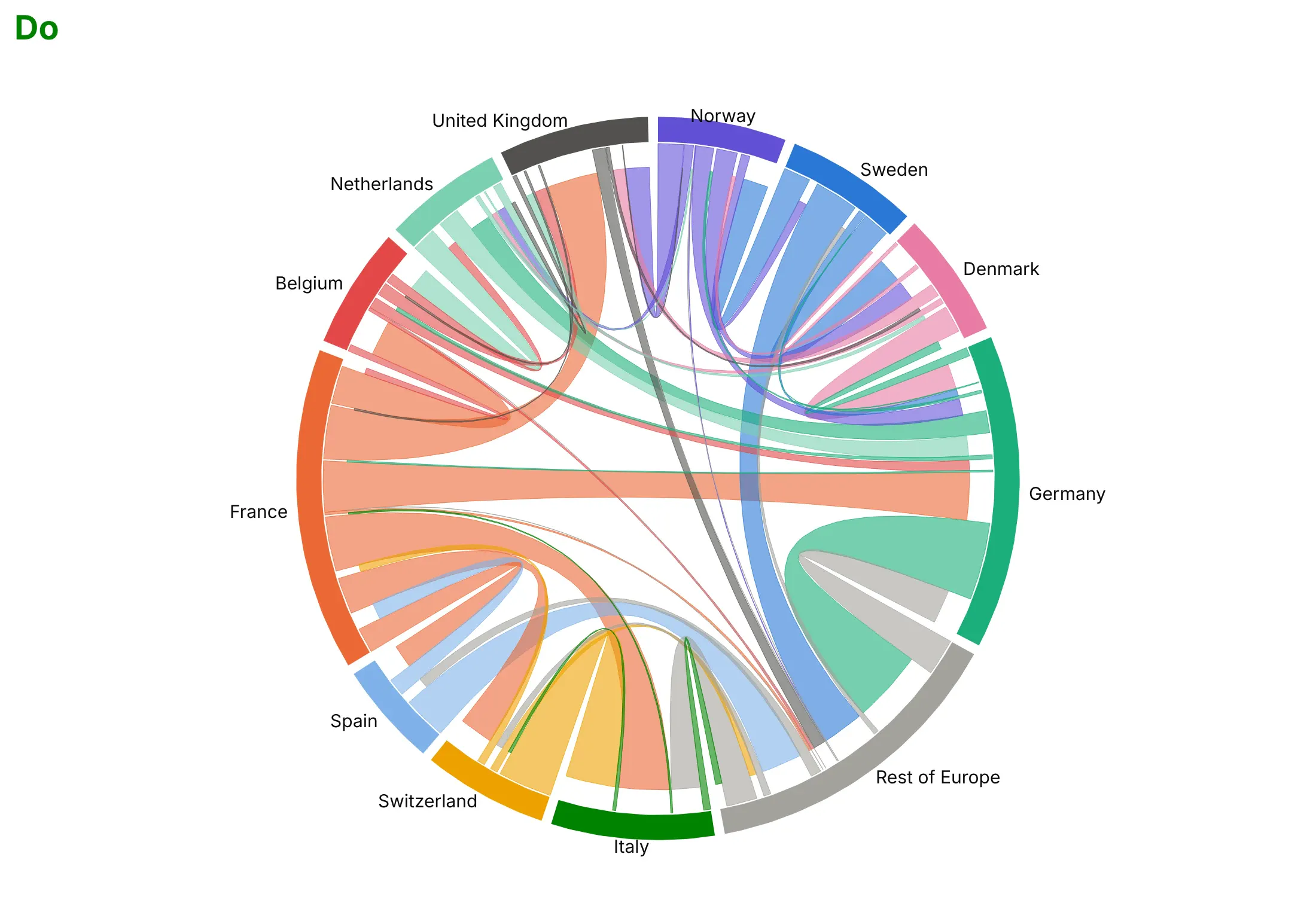
Most of the work in a readable chord diagram is ordering the groups and keeping the ribbons from hiding each other. Here is the European electricity trade both ways, in the same colors.

Don't put the groups in alphabetical order, which scatters neighbors around the circle so trade between them crosses the middle, leave no gaps between the arcs, draw the ribbons opaque so the ones underneath disappear, or use a default serif font:

The European electricity trade with countries in alphabetical order from Belgium to the United Kingdom, no gaps between the arcs, solid opaque ribbons crossing the center in a tangle, and serif labels

Do order the groups so related ones sit together (here by geography, so most ribbons run between neighbors along the edge), leave a small gap between arcs, make the ribbons semi-transparent, and show direction with the short end at the importer:

The same trade with countries in geographic order, white gaps between the arcs, semi-transparent ribbons colored by exporter and mostly running between neighbors, and labels in Inter

Checklist

Order the groups by geography, by type or by a clustering of the matrix, so ribbons between related groups stay short.
Keep it to about 5 to 20 groups, and fold the small ones into one "Other" or "Rest of" group that you name on the chart.
Say whether it's directed, and show direction with color by origin and a gap or arrow at the destination.
Use semi-transparent ribbons, draw the widest first, and put each flow's value in the hover text.
Drop or gray out flows below a threshold when there are hundreds, and state the threshold in the subtitle.
Write a title that states the takeaway, like the largest flow or the biggest net gain.

Don't

Compare arc lengths between two chord diagrams unless they share a scale (example 3 shows how).
Read an undirected co-occurrence chart's arcs as counts of items; one item can add several ribbons.
Use one for flows from one set to a different set, like suppliers to customers; a Sankey reads better.
Use one when readers need exact values; show the matrix as a heatmap or table next to it.

Options to customize

A chord diagram in Plotly is a set of filled go.Scatter traces plus annotations, so these are the options that matter most. The full lists are in the scatter trace reference and the layout reference.

fill="toself": closes each arc and ribbon path and fills it, which is what turns lines into shapes.
fillcolor with an rgba color: the ribbon's color and transparency; 0.5 to 0.7 alpha lets crossings show through.
hoveron="fills", hoverinfo="text", text: hover anywhere on a ribbon to see "France → Italy: 21.9 TWh".
line.width: 0 for clean ribbons, or 0.5 px in a darker shade to separate touching ribbons.
Trace order: traces drawn later sit on top, so add the widest ribbons first, or a highlighted group last.
yaxis.scaleanchor="x" with visible=False: keeps the circle round and hides the axes.
add_annotation(xanchor=...): group labels outside the circle, anchored left on the right half and right on the left half.
Gap between groups: a few degrees of empty circle between arcs (the gap argument of the helper).
Short end at the destination: ending the ribbon at a smaller radius (0.93 in the helper) marks the direction without arrowheads.
A fixed total: drawing two diagrams on the same angle per unit (total= in this guide's full helper) so their arcs compare.
make_subplots: put two chord diagrams side by side, with a separate square x/y axis pair each.
go.Sankey and go.Heatmap: the built-in traces for the two alternatives above.

More chord diagram examples

Six more chord diagrams built from real public data, each with its source, the technique that makes it work and a prompt to rebuild it.

1. Power flows between US grid regions

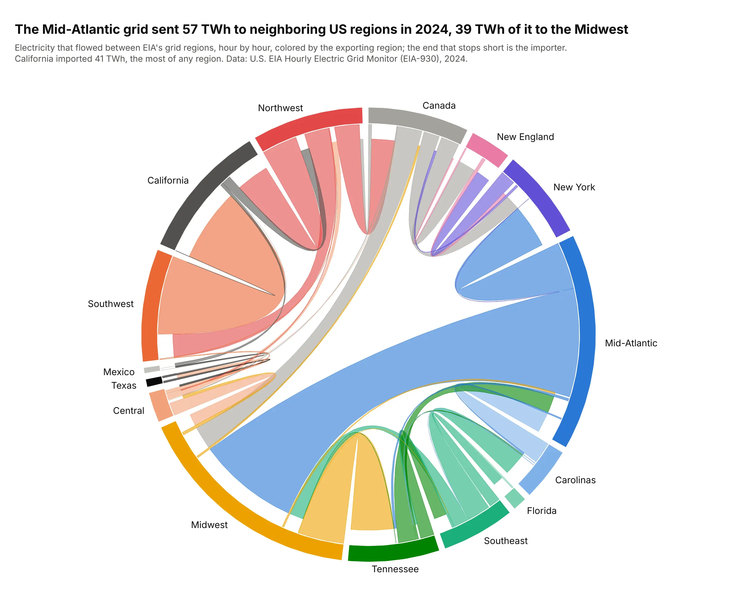
Chord diagram of electricity that flowed between 13 US grid regions, Canada and Mexico in 2024, summed hour by hour; a very wide blue ribbon runs from the Mid-Atlantic to the Midwest, and California's dark gray arc is mostly the short ends of ribbons from the Southwest and Northwest

The Mid-Atlantic region sent 57 TWh of electricity to its neighbors in 2024, 39 TWh of it to the Midwest, and California imported 41 TWh, the most of any region. Texas barely shows, because its grid has few links to the rest of the country. Data: U.S. EIA Hourly Electric Grid Monitor (EIA-930), 2024 interchange files.

Tip: sum hourly flows in the direction each hour's flow went, so borders where power reverses get two ribbons instead of one net number.

Get the data from the US EIA's Hourly Electric Grid Monitor (EIA-930) six-month interchange files for 2024
(columns: Balancing Authority, Directly Interconnected Balancing Authority, Interchange (MW), UTC Time at End
of Hour, Region, DIBA_Region), and shape it into a table (columns: exporter_region, importer_region, gwh).

Build a plotly chord diagram from filled go.Scatter arcs and ribbons: regions in geographic order, ribbons
colored by exporter with the importer's end stopping short of the circle, and flows in TWh on hover.

2. Where Phase 3 trials run

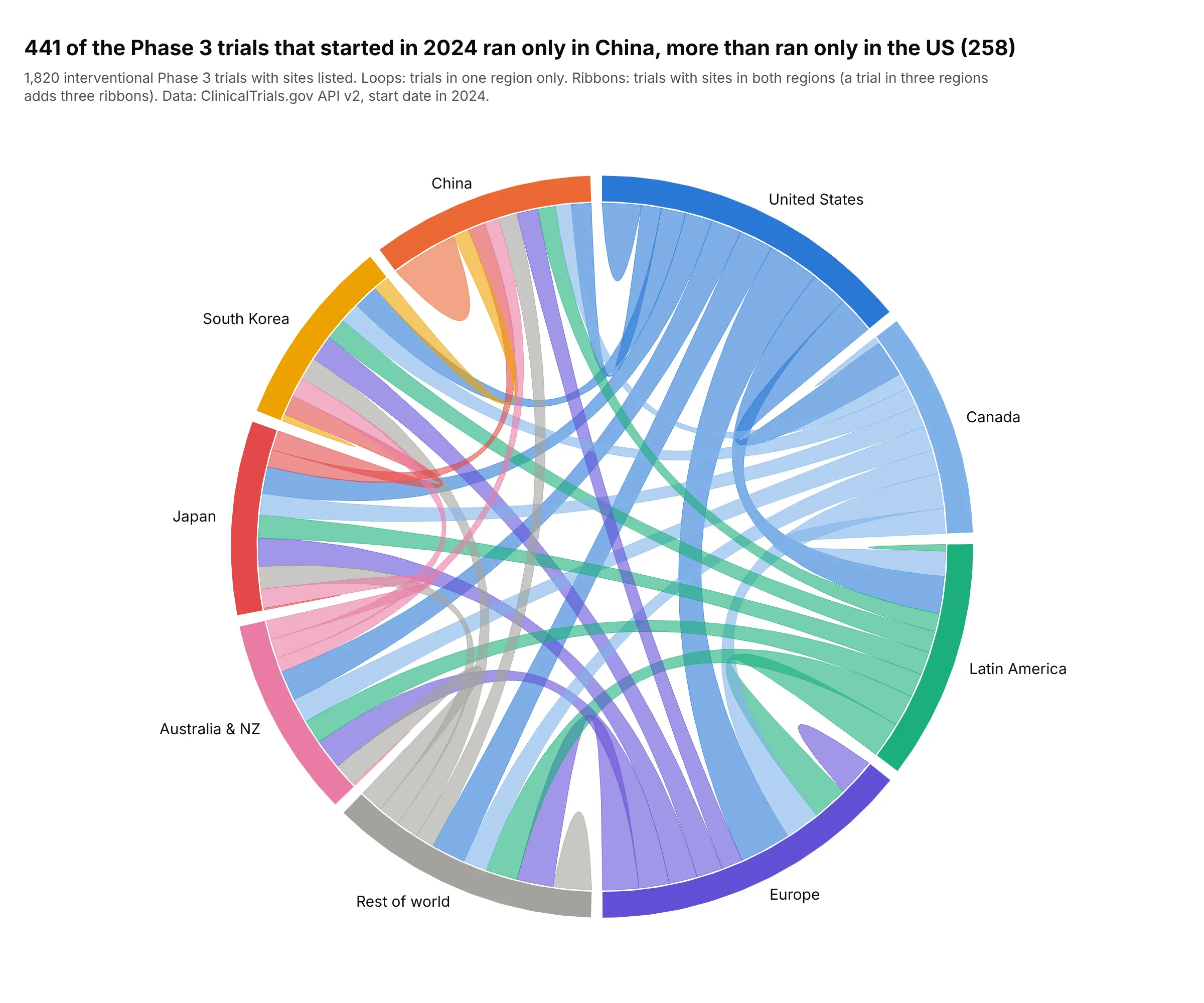
Undirected chord diagram of 1,820 Phase 3 trials that started in 2024 grouped into nine regions; China's orange arc has a large loop for trials run only in China, the United States and Europe have the longest arcs, and blue and purple ribbons run from them to every other region

441 of the Phase 3 trials that started in 2024 ran only in China, against 258 only in the US, and the US and Europe shared sites in 339 trials. The loops show single-region trials and the ribbons show regions that share trials. Data: ClinicalTrials.gov API v2, interventional Phase 3 trials with a 2024 start date.

Tip: in a co-occurrence chord diagram a trial in three regions adds three ribbons, so say in the subtitle that the arcs aren't trial counts.

Get the data from the ClinicalTrials.gov API v2 (interventional Phase 3 studies with a start date in 2024,
fields NCTId and LocationCountry) and shape it into a table (columns: nct_id, country).

Group countries into nine regions, count trials per pair of regions (and trials in one region only on the
diagonal), and build an undirected plotly chord diagram with loops for the diagonal.

3. Global migration then and now, on one scale

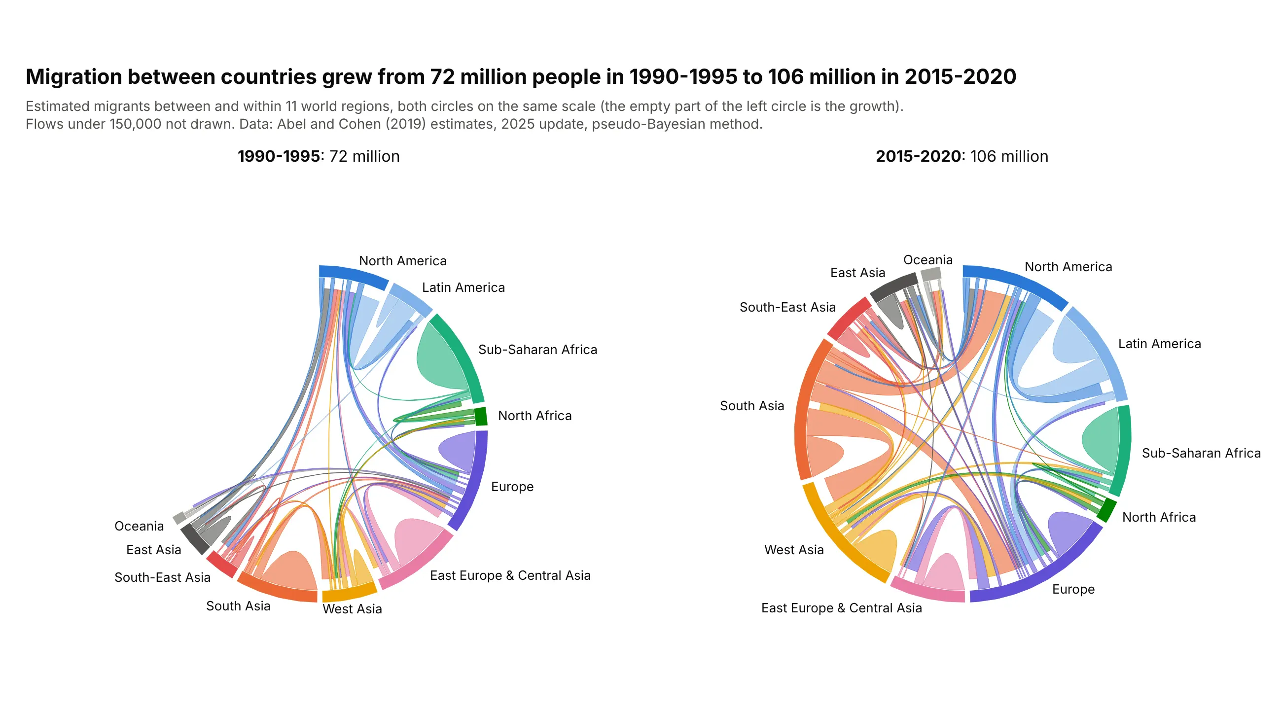
Two chord diagrams of migration between 11 world regions on the same scale: 1990-1995 with 72 million people fills about two thirds of its circle, and 2015-2020 with 106 million fills the whole circle, with wider ribbons from South Asia and into North America and Europe

Migration between countries grew from an estimated 72 million people in 1990-1995 to 106 million in 2015-2020. Both circles use the angle per migrant of the larger period, so the empty part of the left one is the growth. Data: Abel and Cohen (2019) estimates, 2025 update.

Tip: two chord diagrams that each fill the circle hide a change in the total; draw them on a shared scale.

Get the data from Abel and Cohen's bilateral international migration flow estimates on figshare
(doi:10.6084/m9.figshare.7731233, bilat_mig.csv, column da_pb_closed) with the country list's plot_area
regions, and shape it into a table (columns: period, orig_region, dest_region, flow).

Build two plotly chord diagrams side by side with make_subplots for 1990-1995 and 2015-2020, with the same
angle per migrant in both, regions in the same order and colors.

4. Moves between US states

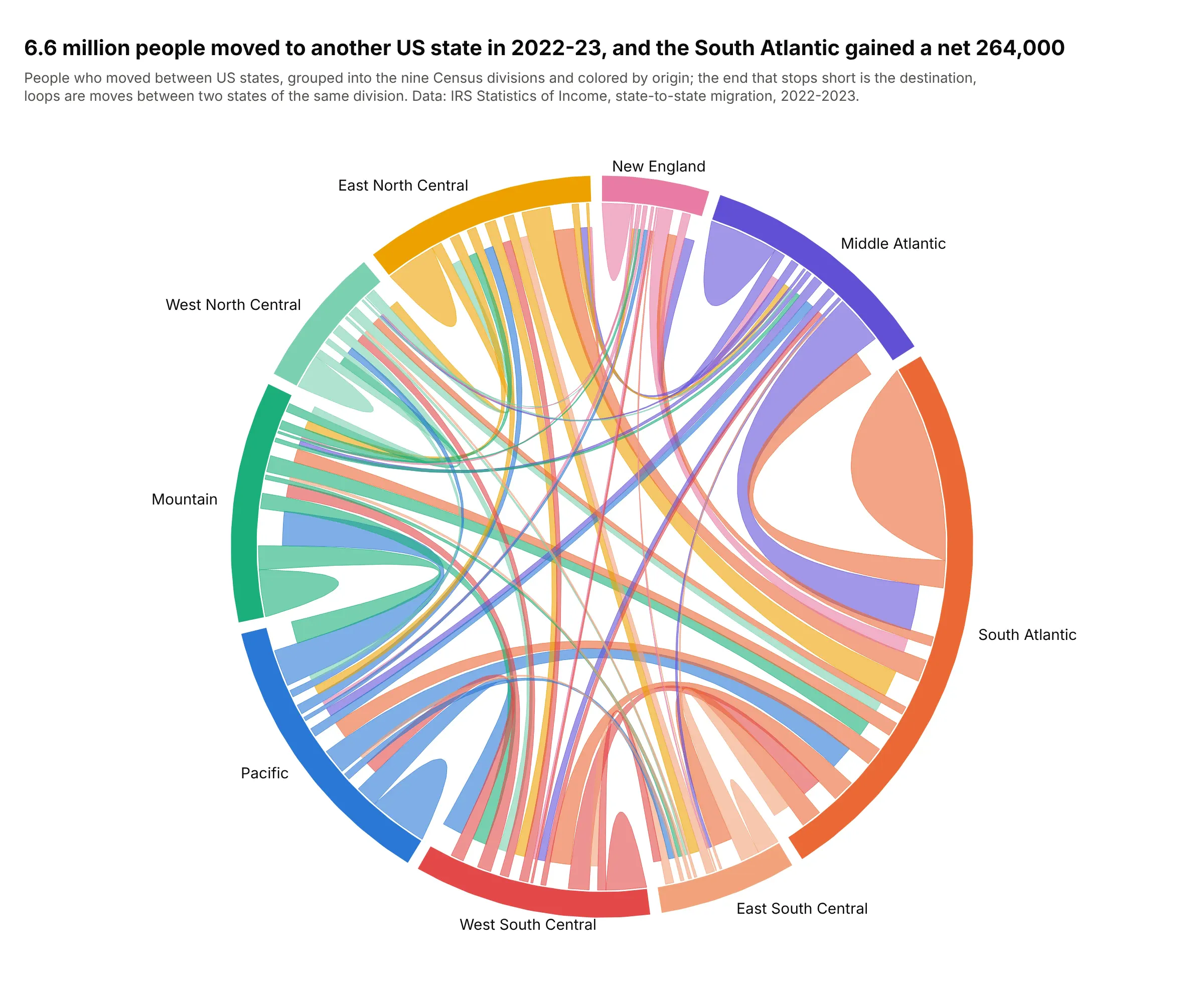
Chord diagram of 6.6 million people who moved between US states in 2022-23, grouped into nine Census divisions; the South Atlantic's orange arc is the longest with a large loop for moves within it, and wide ribbons come into it from the Middle Atlantic and East North Central

6.6 million people moved to another US state between their 2022 and 2023 tax returns, and the South Atlantic gained a net 264,000 of them. The biggest single ribbon into it, 319,000 people, came from the Middle Atlantic. Data: IRS Statistics of Income, state-to-state migration data, 2022-2023.

Tip: a chord diagram shows the gross flows in both directions behind a net number, which a map of net migration hides.

Get the data from the IRS Statistics of Income state-to-state migration outflow file for 2022-2023
(stateoutflow2223.csv; columns y1_statefips, y2_statefips, y2_state, n1, n2) and shape it into a table
(columns: origin, destination, individuals).

Group states into the nine Census divisions and build a directed plotly chord diagram, ribbons colored by
origin, loops for moves within a division, and the net gain of each division in the hover text.

5. A dependency wheel of Python data libraries

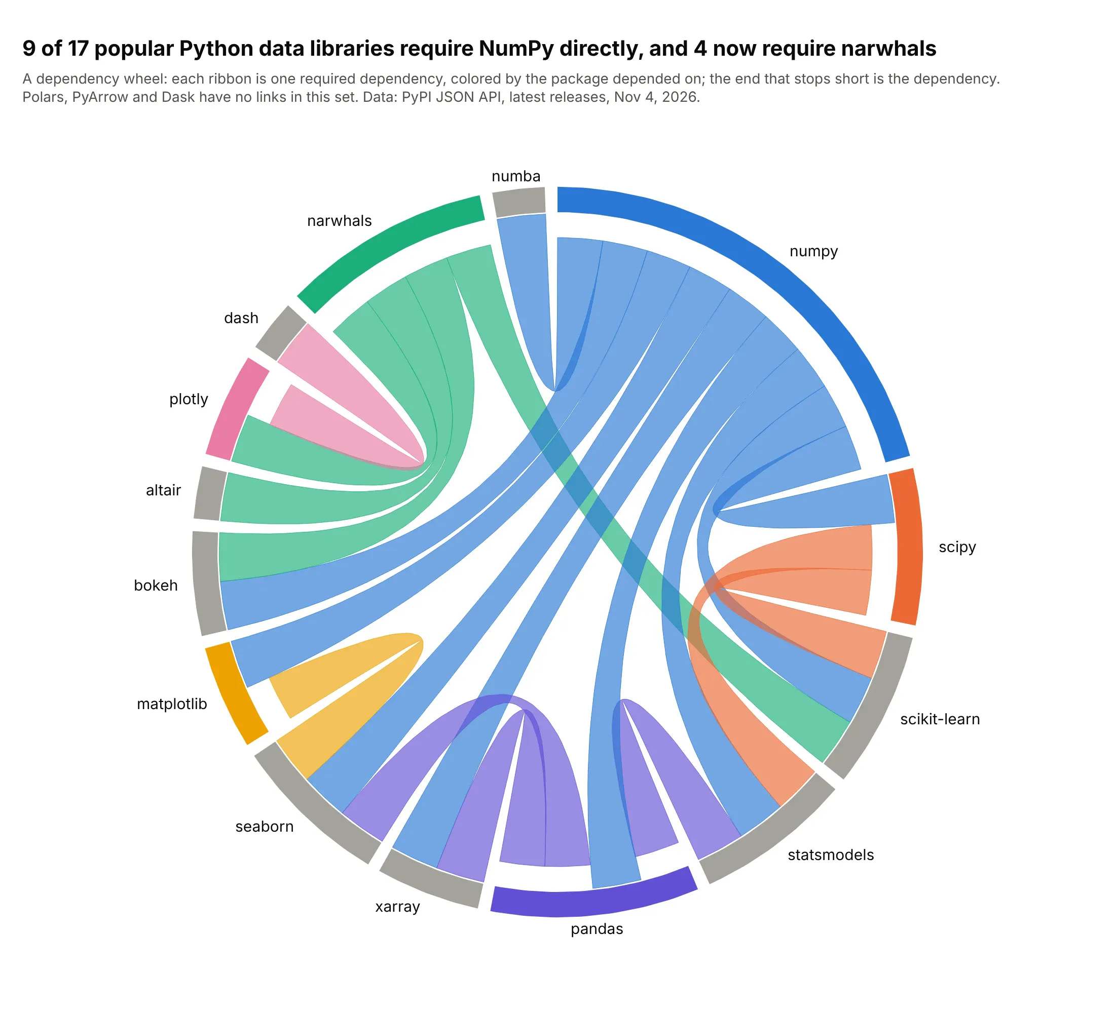
Dependency wheel of 14 Python data libraries: NumPy's blue arc is the largest with blue ribbons from pandas, SciPy, scikit-learn, statsmodels, matplotlib, seaborn, xarray, numba and bokeh, and narwhals' green ribbons come from plotly, altair, bokeh and scikit-learn

9 of 17 popular Python data libraries require NumPy directly, and 4 (plotly, altair, bokeh and scikit-learn) require narwhals, the dataframe compatibility layer. With every link the same width, an arc's length is its number of links. Data: PyPI JSON API, latest releases on November 4, 2026.

Tip: color each ribbon by the package depended on, so the libraries everything rests on show as fans of one color.

Get the data from the PyPI JSON API (pypi.org/pypi/<package>/json, info.requires_dist without extras) for
numpy, pandas, scipy, matplotlib, seaborn, scikit-learn, statsmodels, plotly, dash, polars, pyarrow,
narwhals, xarray, dask, numba, altair and bokeh, and shape it into a table (columns: package, depends_on).

Build a plotly dependency wheel (a chord diagram with one ribbon per dependency), ribbons colored by the
package depended on.

6. Airline routes between world regions

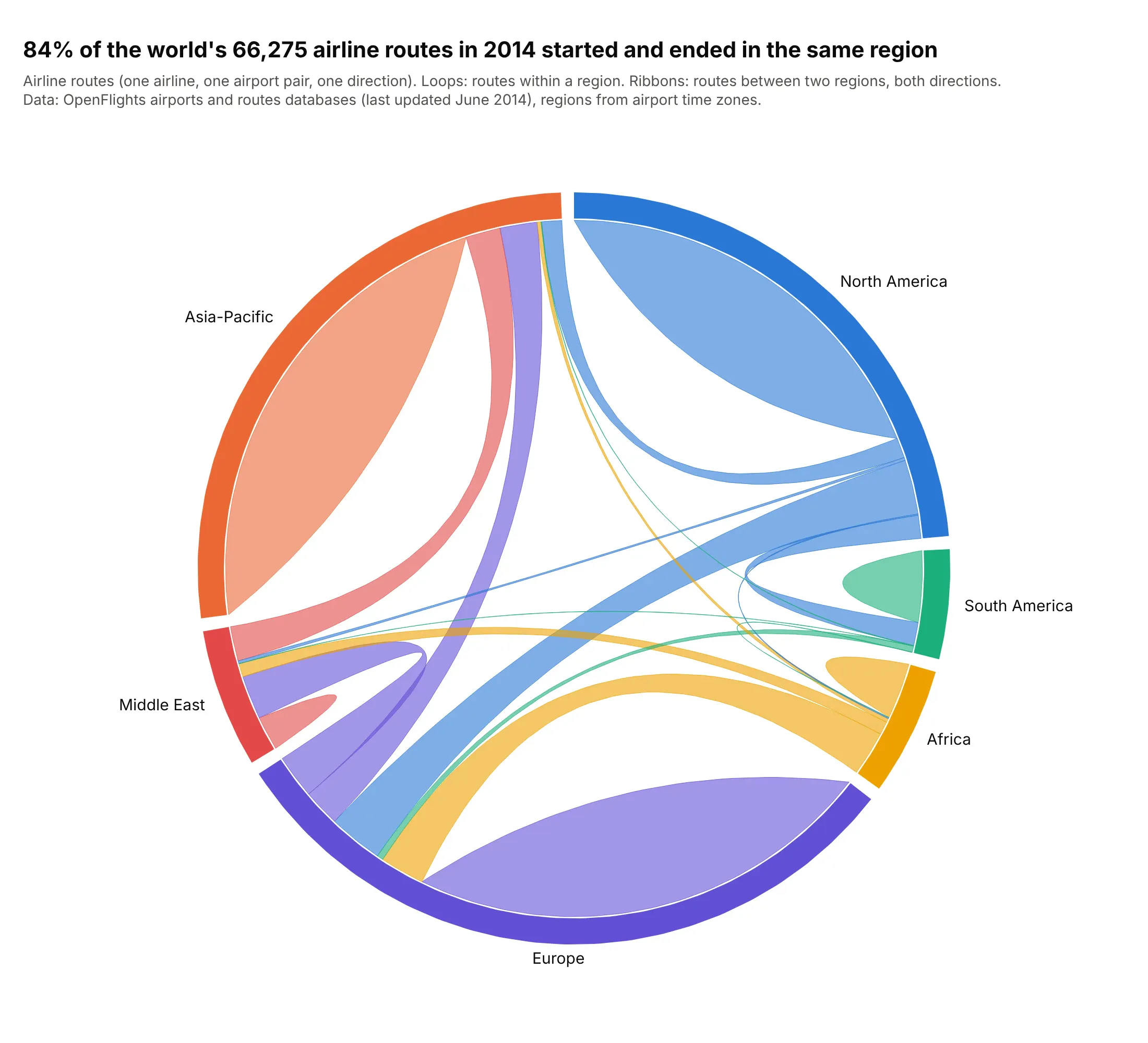
Chord diagram of 66,275 airline routes in six world regions; large loops for routes within Europe, Asia-Pacific and North America take up most of the circle, and thinner ribbons connect Europe with North America, Africa, the Middle East and Asia-Pacific

84% of the world's 66,275 airline routes in OpenFlights' 2014 database started and ended in the same region, so the loops take up most of the circle. Europe to North America is the busiest link between regions, with about 1,000 routes each way. Data: OpenFlights airport and route databases (last updated June 2014).

Tip: when loops dominate, say so in the title, or draw a second chart without them to show the links between groups.

Get the data from the OpenFlights route and airport databases (github.com/jpatokal/openflights,
routes.dat and airports.dat; columns: source and destination airport IDs, airport time zone, latitude,
longitude) and shape it into a table (columns: from_region, to_region, routes).

Build an undirected plotly chord diagram of routes between six world regions, with loops for routes
within a region and route counts on hover.