Chris Parmer

November 12, 2026

ROC Curves - A Complete Guide

TL;DR

A receiver operating characteristic (ROC) curve shows how well a test or a model separates two groups, such as patients with and without a disease, at every possible cutoff. Each point is one cutoff, drawn at its false positive rate (1 − specificity) on the x axis and its true positive rate (sensitivity) on the y axis.
ROC curves are also known as receiver operating characteristic curves, relative operating characteristic curves and sensitivity vs (1 − specificity) plots. They are similar to precision-recall curves, detection error tradeoff (DET) curves and empirical cumulative distribution function (ECDF) plots of the two groups.
The diagonal is chance, and the area under the curve (AUC) sums the curve up in one number: 0.5 is a coin flip, 1.0 is perfect, and it equals the chance that a random positive case scores higher than a random negative one.
They started with radar receivers in World War II, moved into psychology and radiology, and are now the standard chart for diagnostic tests and for comparing machine learning classifiers. With rare positives, pair them with a precision-recall curve.
You can make an ROC curve with Plotly in Python from scikit-learn's roc_curve, which returns the false and true positive rates at every cutoff, and a go.Scatter trace with a dashed diagonal.

What is an ROC curve?

ROC curves look like this:

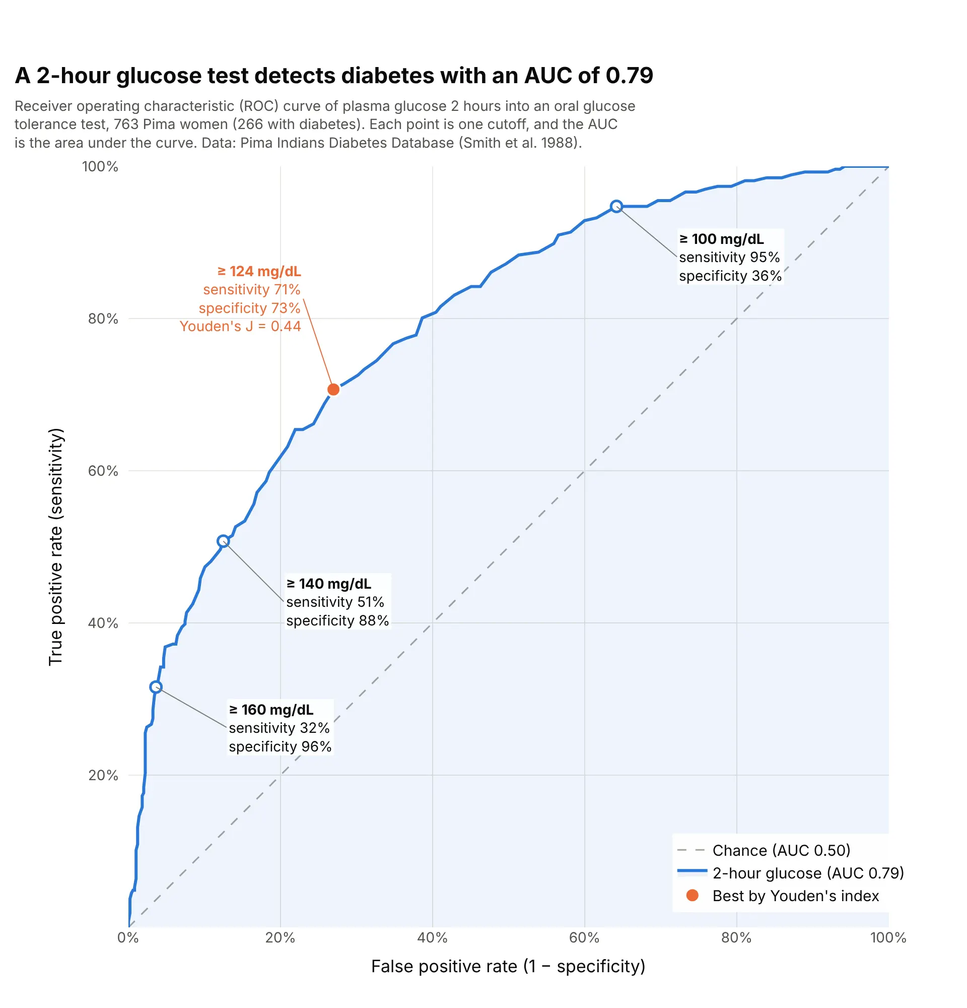
ROC curve of the 2-hour glucose test for diabetes in 763 Pima women, AUC 0.79: a blue curve rising steeply from the bottom-left corner and bending over toward the top right, well above a dashed diagonal, with cutoffs labeled at 160 mg/dL (sensitivity 32%, specificity 96%), 140 (51%, 88%), 100 (95%, 36%) and Youden's best cutoff of 124 mg/dL in orange (71%, 73%)

Data: Pima Indians Diabetes Database (National Institute of Diabetes and Digestive and Kidney Diseases; Smith et al. 1988), via the Plotly datasets repository.

How do you read an ROC curve? In the example above, notice these things:

Each point on the curve is one cutoff for calling a test positive. At "glucose of 140 mg/dL or more", the test finds 51% of the 266 women with diabetes (sensitivity, on the y axis) and wrongly flags 12% of the 497 without it (the false positive rate, 1 − specificity, on the x axis).
Lowering the cutoff moves you up and to the right along the curve: at 100 mg/dL the test catches 95% of the women with diabetes but flags 64% of those without, so specificity falls to 36%.
The dashed diagonal is what a test with no information would give, such as flipping a coin. The further the curve bows toward the top-left corner, the better the test separates the groups.
The area under the curve is 0.79, which means that a randomly chosen woman with diabetes has a higher glucose than a randomly chosen woman without it 79% of the time, counting ties as half. The orange point at 124 mg/dL has the highest Youden's index, sensitivity plus specificity minus 1, here 0.44.

It's often used for charts like these:

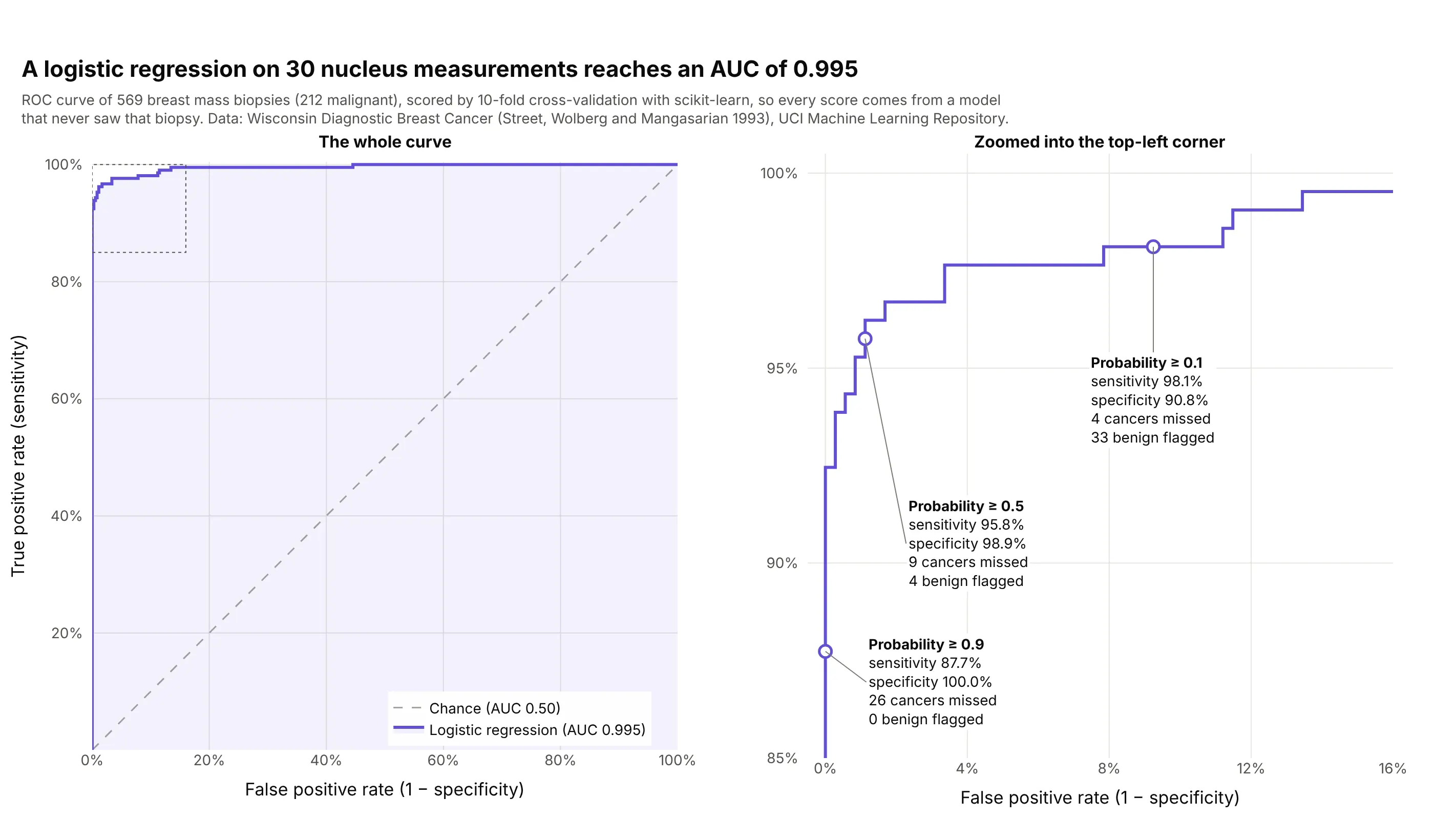
Two ROC curves of a logistic regression on the Wisconsin breast cancer data, AUC 0.995: the whole curve hugging the top-left corner, and a zoom of that corner showing cutoffs 0.9 (sensitivity 87.7%, specificity 100%, 26 cancers missed), 0.5 (95.8%, 98.9%, 9 missed and 4 benign flagged) and 0.1 (98.1%, 90.8%, 4 missed and 33 benign flagged)

Evaluating a machine learning model. A logistic regression trained with scikit-learn on 30 measurements of cell nuclei separates 212 malignant from 357 benign breast biopsies with an AUC of 0.995, and its default cutoff of 0.5 misses 9 cancers. Data: Wisconsin Diagnostic Breast Cancer (Street, Wolberg and Mangasarian 1993), UCI Machine Learning Repository.

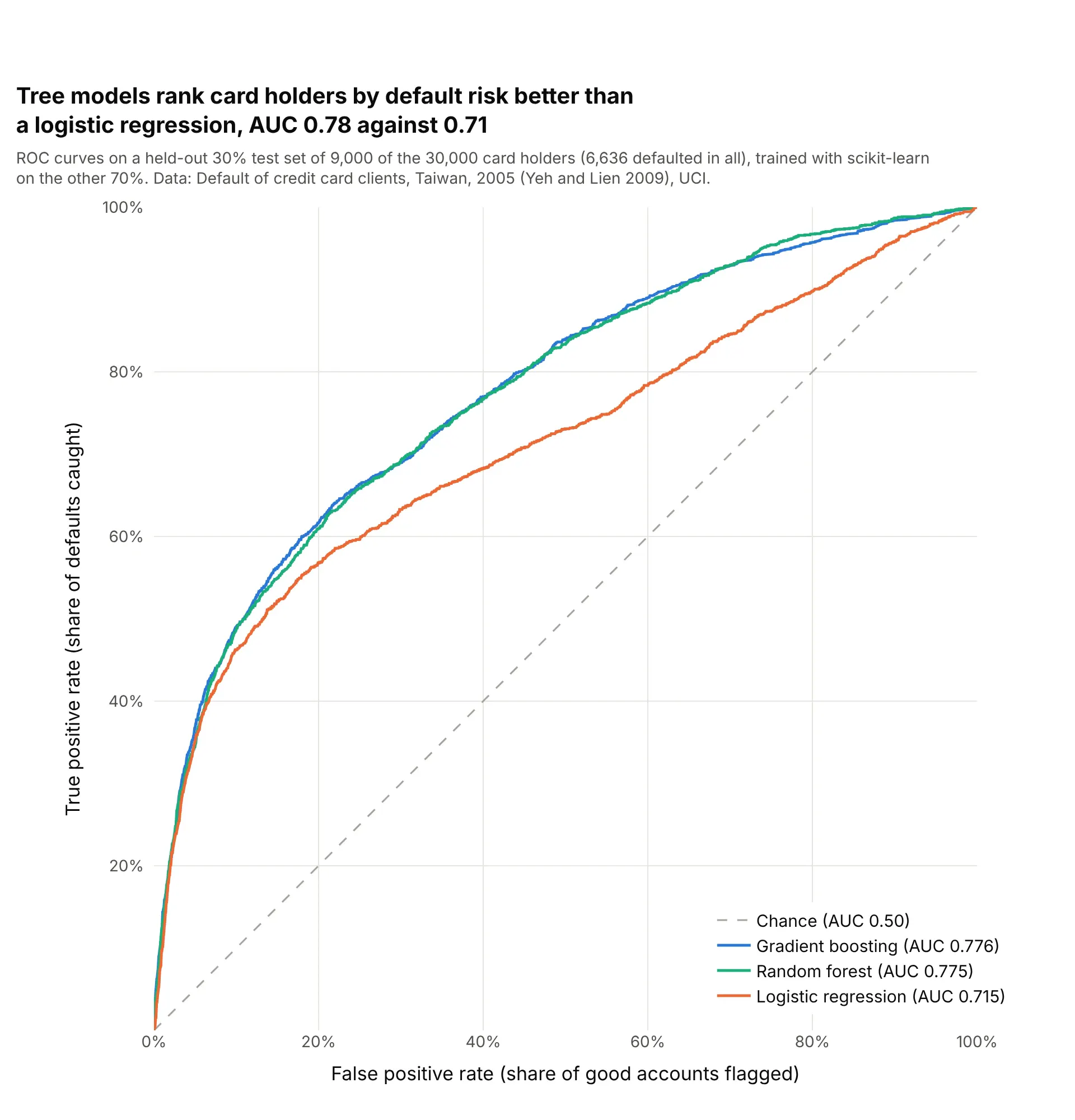
ROC curves of three scikit-learn models predicting credit card default on 9,000 held-out card holders: gradient boosting (AUC 0.78) and random forest (0.78) almost on top of each other and above logistic regression (0.71), all above the dashed diagonal

Comparing models in finance. On the same 9,000 held-out card holders, gradient boosting and a random forest rank defaulters above good accounts with an AUC of 0.78, against 0.71 for a logistic regression. Data: Default of credit card clients, Taiwan, 2005 (Yeh and Lien 2009), UCI.

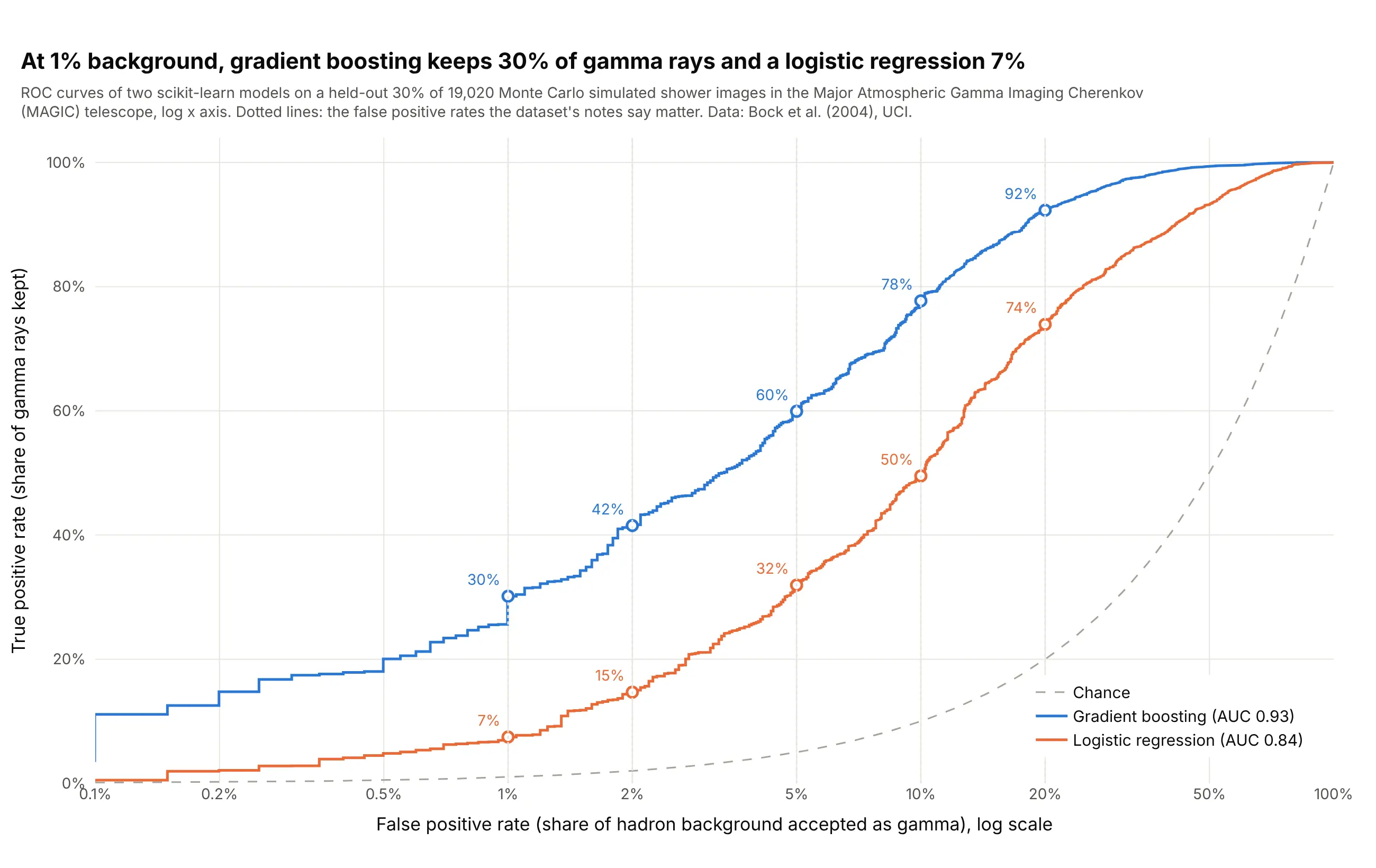
ROC curves on a log false-positive axis for separating gamma rays from cosmic-ray background in the MAGIC telescope: at 1% background accepted, gradient boosting keeps 30% of gamma rays and logistic regression 7%, with dotted lines and labeled points at 1%, 2%, 5%, 10% and 20%

Signal detection in physics. Telescope teams read the curve at a fixed, small rate of background: at 1% of cosmic-ray showers accepted, gradient boosting keeps 30% of gamma rays and a logistic regression 7%, a difference the AUCs (0.93 and 0.84) understate. Data: gamma telescope data 2004 from the Major Atmospheric Gamma Imaging Cherenkov telescope (Bock et al. 2004), Monte Carlo simulated events, UCI.

ROC curves explained: sensitivity, specificity and thresholds

An ROC curve assumes a few ideas from diagnostic testing. Most tests and models don't say yes or no; they give a number, such as a glucose reading or a predicted probability, and somebody picks a cutoff (also called a threshold) above which the result counts as positive. Everything on the chart follows from that choice.

One cutoff makes four counts

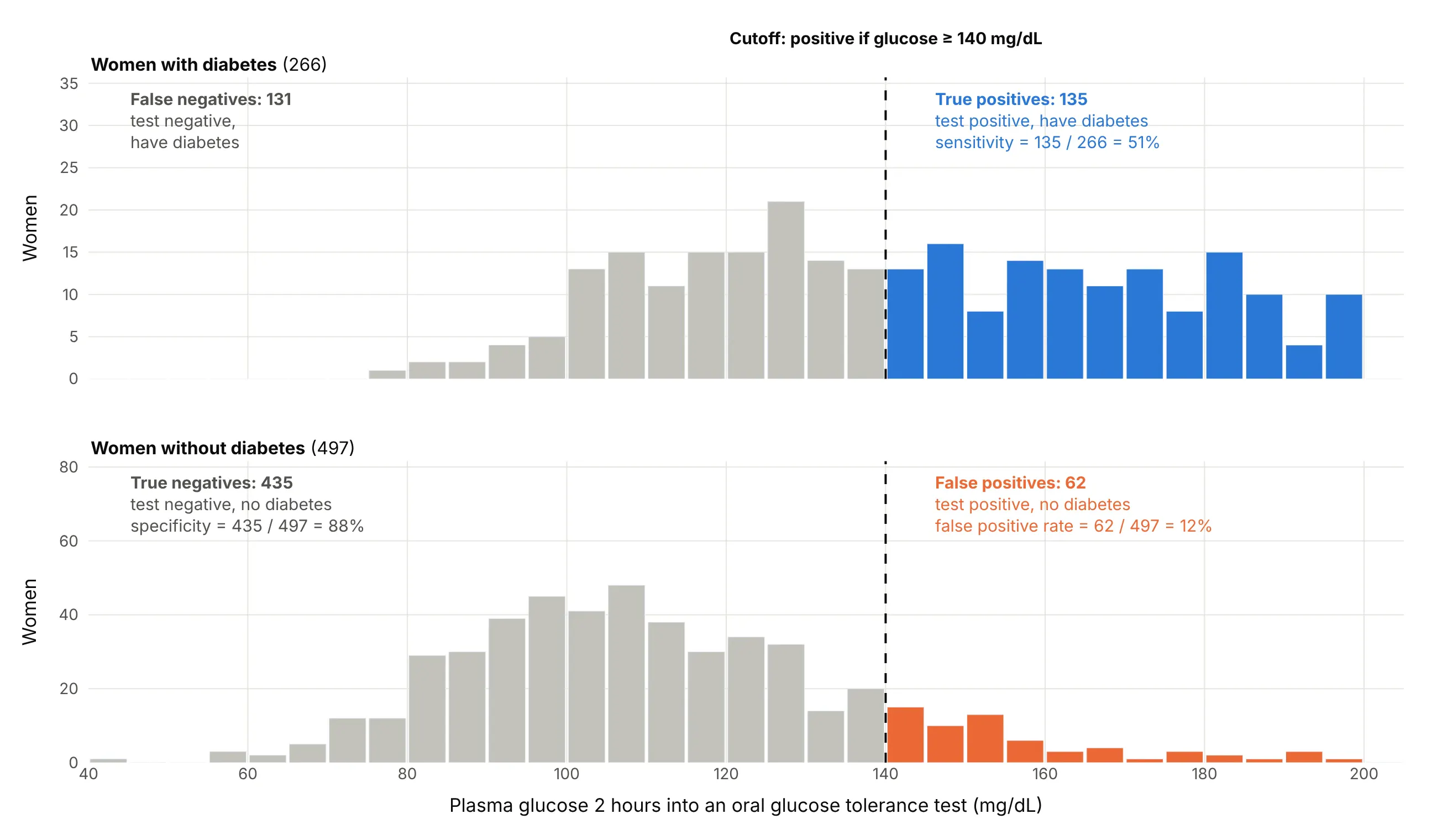
Take the glucose test and a cutoff of 140 mg/dL. The women with diabetes split into those above the cutoff, the true positives, and those below it, the false negatives, the cases the test misses. The women without diabetes split into false positives above the cutoff and true negatives below it:

Two histograms of 2-hour glucose with a dashed cutoff at 140 mg/dL: for the 266 women with diabetes, 135 true positives above it in blue and 131 false negatives below it; for the 497 women without diabetes, 62 false positives above it in orange and 435 true negatives below it

Data: Pima Indians Diabetes Database (Smith et al. 1988).

Two rates describe the result, each computed within one group:

Sensitivity, or the true positive rate, or recall, is the share of the sick who test positive: 135 of 266, or 51%.
Specificity is the share of the healthy who test negative: 435 of 497, or 88%. Its complement, 1 − specificity, is the false positive rate: 62 of 497, or 12%.

That cutoff is the point (12%, 51%) on the ROC curve above.

Moving the cutoff trades one for the other

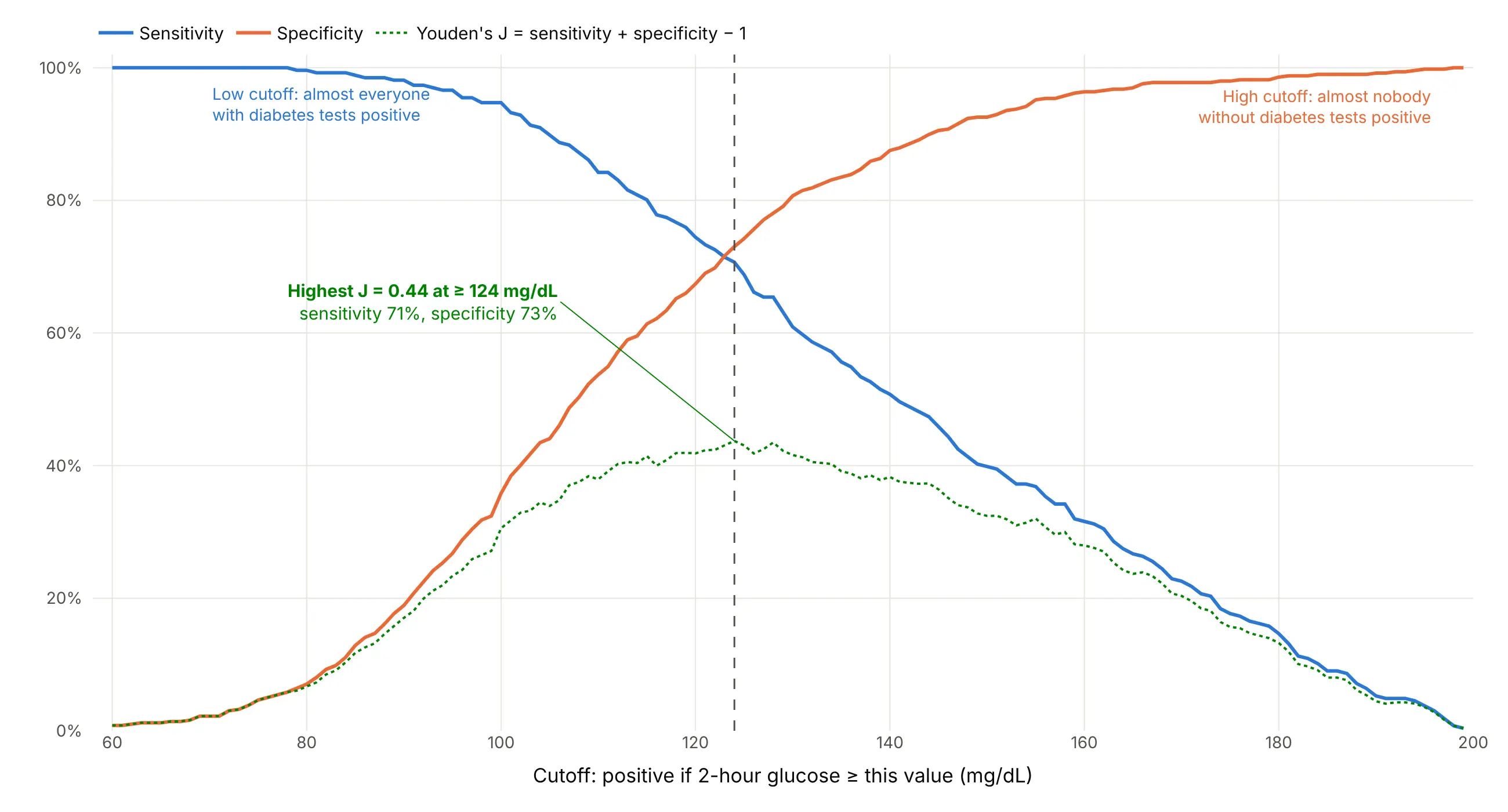
A lower cutoff catches more of the sick and flags more of the healthy, so sensitivity rises while specificity falls. Drawing both against every cutoff from 60 to 199 mg/dL shows the trade:

Sensitivity falling from 100% and specificity rising from 0% as the glucose cutoff goes from 60 to 200 mg/dL, crossing near 124 mg/dL, where a dotted green line of Youden's J peaks at 0.44 with sensitivity 71% and specificity 73%

Data: Pima Indians Diabetes Database (Smith et al. 1988).

An ROC curve is this same chart with the cutoff axis taken away: each cutoff becomes one point, at its false positive rate and its sensitivity. That's why ROC curves compare tests measured in different units, such as glucose in mg/dL and a model's probability, on one chart.

Choosing a cutoff with Youden's index

If missing a case and raising a false alarm cost about the same, a common choice is the cutoff with the highest Youden's index (J), sensitivity + specificity − 1, proposed by W. J. Youden in 1950 (Youden 1950). On the ROC curve it is the point farthest above the diagonal. For glucose it is 124 mg/dL, with J = 0.44. When the costs differ, as in screening for a serious disease, pick a cutoff with high sensitivity instead, and accept more false positives.

What the area under the curve means

The AUC is the area under the curve, from 0.5 for the diagonal to 1 for a curve through the top-left corner. It has a plain meaning: it is the probability that a randomly chosen positive case gets a higher score than a randomly chosen negative case, which is the Mann-Whitney U (Wilcoxon) statistic scaled to 0 to 1 (Hanley and McNeil 1982). An AUC of 0.79 means that in 79% of pairs of a woman with diabetes and one without, the one with diabetes has the higher glucose, counting ties as half. It says nothing about any single cutoff, so a report should give both the AUC and the sensitivity and specificity at the cutoff that will be used.

What ROC curves look like

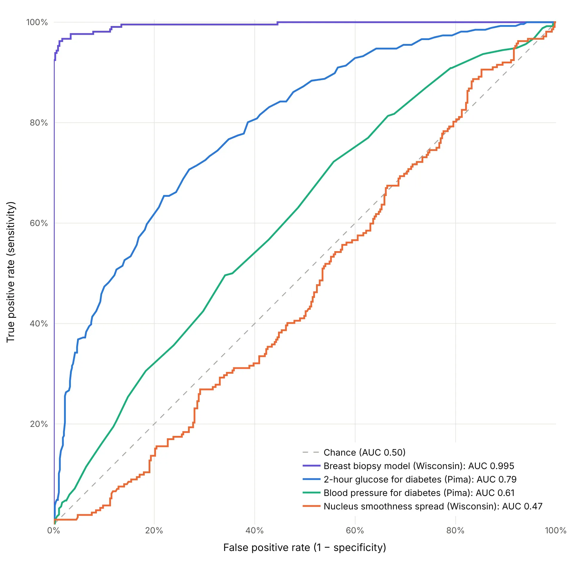
These four real scores range from almost perfect to no better than chance:

Four ROC curves on one chart: the Wisconsin breast biopsy model hugging the top-left corner (AUC 0.995), 2-hour glucose for diabetes bowing well above the diagonal (0.79), blood pressure for diabetes a little above it (0.61), and the spread of nucleus smoothness in the Wisconsin data crossing the diagonal (0.47)

Data: Wisconsin Diagnostic Breast Cancer (Street, Wolberg and Mangasarian 1993) and Pima Indians Diabetes Database (Smith et al. 1988).

Near the top-left corner (AUC above 0.95): almost every cutoff in the corner finds nearly all positives with few false alarms. Check that the model wasn't scored on its own training data (example 5 below).
A smooth bow (0.7 to 0.9): a useful test with real overlap between the groups, the common case for lab values and credit models.
Close to the diagonal (about 0.5 to 0.65): the score carries little information on its own, like blood pressure for diabetes.
Below the diagonal (under 0.5): the score runs the wrong way for this question. Flipping its sign gives 1 − AUC, so a curve far below the diagonal is informative, just backwards.
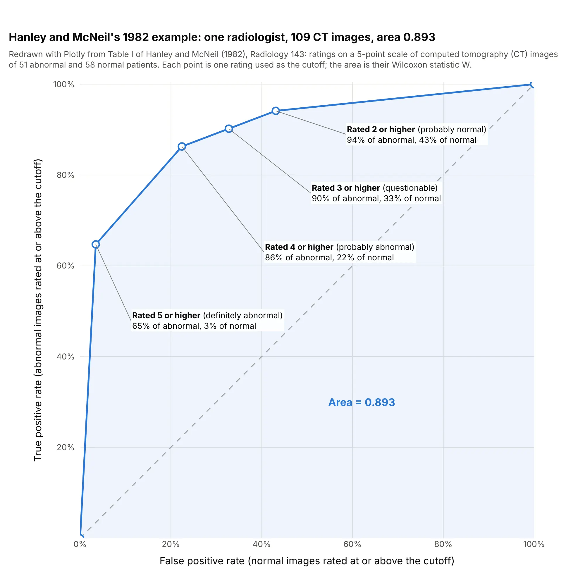
Long straight segments come from ties: a 5-point rating scale or a rounded lab value gives only a handful of distinct cutoffs, joined by straight lines.

A short history

The name comes from radar. In World War II, engineers measured how well radar receiver operators told aircraft echoes from noise, and the "receiver operating characteristic" described that trade between hits and false alarms (Wikipedia, which cites Green and Swets's 1966 book Signal Detection Theory and Psychophysics). In 1954 Peterson, Birdsall and Fox set out the theory of signal detectability, and Tanner and Swets applied it to human visual detection the same year, which brought ROC curves into psychology. Lee Lusted's 1971 Science article, "Signal Detectability and Medical Decision-Making", carried the idea into medicine, and John Swets's 1988 Science article, "Measuring the Accuracy of Diagnostic Systems", applied it to diagnostic systems in general. Hanley and McNeil's 1982 Radiology paper showed that the area under the curve is the Wilcoxon statistic and how to compute its standard error, using one radiologist's ratings of 109 computed tomography (CT) images. Their table is public in the paper, so here it is redrawn:

ROC curve redrawn from Hanley and McNeil's 1982 Table I: five points for ratings of 5 (definitely abnormal) down to 2 (probably normal), at 65% of abnormal and 3% of normal images, 86% and 22%, 90% and 33%, and 94% and 43%, joined by straight lines above the diagonal, with an area of 0.893

Data: Hanley and McNeil (1982), Table I, typed from the paper.

Machine learning picked up ROC analysis in the 1990s (Bradley 1997), and Tom Fawcett's 2006 introduction is a widely cited guide to computing and averaging the curves.

Alternatives to an ROC curve

Here's the same glucose test drawn six ways. Some are better for the question, some worse, some just different:

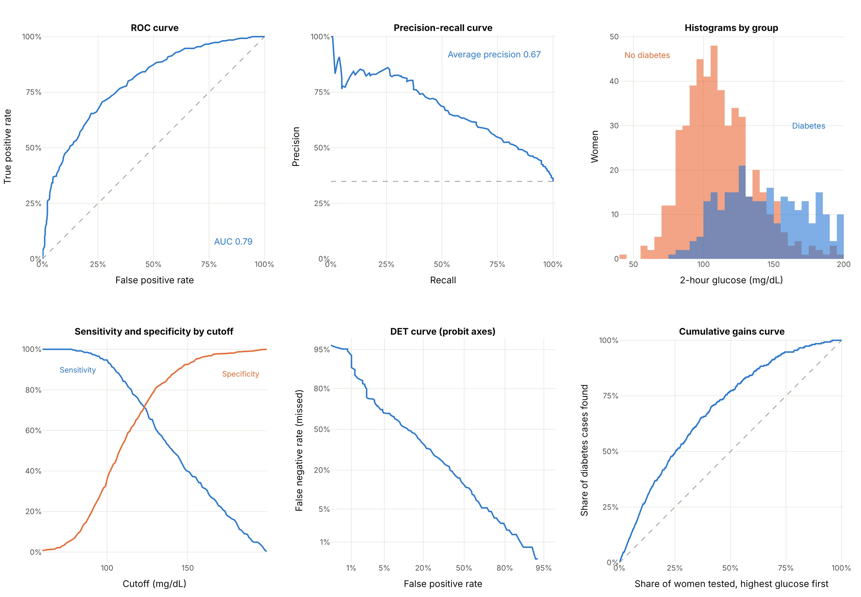
The Pima glucose test drawn six ways: an ROC curve with AUC 0.79, a precision-recall curve falling from about 85% precision to 35% with average precision 0.67, overlapping histograms of glucose for women with and without diabetes, sensitivity and specificity against the cutoff, a detection error tradeoff curve on probit axes that is nearly a straight line, and a cumulative gains curve above its diagonal

Precision-recall curve (better when positives are rare). It plots the share of flagged cases that are real (precision) against sensitivity (recall). Because precision depends on how common the positives are, it shows what an ROC curve hides when they are rare (Saito and Rehmsmeier 2015); example 1 below draws both. Its no-skill line is the share of positives, here 35%, not a diagonal.
Histograms of the score by group (works too, and better for explaining). They show the overlap that the ROC curve summarizes, and where a cutoff would fall, but comparing two tests needs two charts.
Sensitivity and specificity by cutoff (better for picking a cutoff). The cutoff is on the x axis in the test's own units, so you can read the value to use. It can't compare tests measured in different units.
Detection error tradeoff (DET) curve (different). It plots the miss rate against the false positive rate on probit (normal quantile) axes, which spreads out the low-error corners and turns a normal-shaped test into a straight line. It was introduced for evaluating speech technology at the Eurospeech 1997 conference.
Cumulative gains or lift curve (different). It plots the share of positives found against the share of cases checked, highest score first, which answers "if we test the top 20%, how many cases do we find?"
Confusion matrix (worse on its own). A 2 by 2 table of the four counts at one cutoff, such as the 135, 131, 62 and 435 above, gives exact numbers but no view of the other cutoffs.

How to make an ROC curve

With AI

ChatGPT, Claude Code, GitHub Copilot, Cursor and other AI tools are excellent at writing Plotly code. Name Plotly in the prompt, and say how the scores are computed so the curve isn't scored on training data:

Make a plotly ROC curve from scores.csv (columns: id, label with 1 for positive and 0 for negative,
score from a model where higher means more likely positive).

- Compute the curve with sklearn.metrics.roc_curve and the area with roc_auc_score.
- Square plot area (yaxis scaleanchor="x"), both axes 0 to 1 as percentages, x titled
  "False positive rate (1 − specificity)" and y "True positive rate (sensitivity)".
- A dashed diagonal for chance, the AUC to 3 decimals in the legend, and the cutoff in the hover text.
- Mark the cutoff with the highest Youden's index (tpr − fpr) and label its sensitivity and specificity.
- Check: print the AUC, the best cutoff and its sensitivity and specificity, and the number of
  positives and negatives.

With Plotly Studio

Plotly Studio is a desktop app where you point an AI at a dataset and it builds charts and a Dash app around your questions. Ask for an ROC curve the same way:

Train a logistic regression and a gradient boosting model to predict default from the other columns, and show their ROC curves on held-out data with the AUC of each in the legend, a slider for the cutoff that moves a marker along each curve, and a table of sensitivity, specificity and precision at that cutoff.

Make an ROC curve in Python or JavaScript

This is the code AI tools write under the hood. In Python, scikit-learn's roc_curve returns the false positive rate, the true positive rate and the cutoff at every point, and roc_auc_score the area. Plotly draws the curve as a scatter trace with a line. This example trains a model on the Wisconsin breast cancer data, which ships with scikit-learn:

import plotly.graph_objects as go
from sklearn.datasets import load_breast_cancer
from sklearn.linear_model import LogisticRegression
from sklearn.metrics import roc_auc_score, roc_curve
from sklearn.model_selection import train_test_split
from sklearn.pipeline import make_pipeline
from sklearn.preprocessing import StandardScaler

X, y = load_breast_cancer(return_X_y=True)  # the Wisconsin data; in scikit-learn, 1 = benign
y = 1 - y                                   # make malignant the positive class

X_train, X_test, y_train, y_test = train_test_split(X, y, test_size=0.3, stratify=y, random_state=0)
model = make_pipeline(StandardScaler(), LogisticRegression(max_iter=5000)).fit(X_train, y_train)
scores = model.predict_proba(X_test)[:, 1]  # probability of the positive class

fpr, tpr, thresholds = roc_curve(y_test, scores)
auc = roc_auc_score(y_test, scores)

fig = go.Figure([
    go.Scatter(x=[0, 1], y=[0, 1], mode="lines", line=dict(dash="dash", color="gray"), name="Chance"),
    go.Scatter(x=fpr, y=tpr, mode="lines", name=f"Logistic regression (AUC {auc:.3f})",
               customdata=thresholds, hovertemplate="Cutoff %{customdata:.2f}<br>FPR %{x:.2f}<br>TPR %{y:.2f}"),
])
fig.update_layout(
    xaxis=dict(title="False positive rate (1 − specificity)", range=[0, 1], constrain="domain"),
    yaxis=dict(title="True positive rate (sensitivity)", range=[0, 1], scaleanchor="x", constrain="domain"),
    width=700, height=700,
)
fig.show()

On this 30% test split the AUC is 0.992. scaleanchor="x" keeps the plot square, so the diagonal is at 45°. Pass the scores, not the 0 or 1 predictions from model.predict: with predictions alone, the curve has a single cutoff and the AUC means little. For a single test such as a lab value, pass the measurement itself as the score. sklearn.metrics.RocCurveDisplay draws the same curve with matplotlib; using roc_curve and Plotly gives you hover labels with the cutoff, zoom into the corner and a chart that drops into a Dash app. For a precision-recall curve, swap in precision_recall_curve and average_precision_score.

In JavaScript, plotly.js draws an ROC curve from a scatter trace once you've counted the positives and negatives at each cutoff. This one uses the rating table from Hanley and McNeil's 1982 paper:

<div id="chart"></div>
<script src="https://cdn.plot.ly/plotly-4.1.1.min.js"></script>
<script>
  // One radiologist's ratings of 109 CT images (Hanley and McNeil 1982, Table I),
  // from 5 (definitely abnormal) down to 1 (definitely normal)
  const ratings = [5, 4, 3, 2, 1];
  const abnormal = [33, 11, 2, 2, 3];   // 51 patients with disease
  const normal = [2, 11, 6, 6, 33];     // 58 patients without

  // Each rating used as a cutoff ("positive if rated this or higher") gives one point
  const total = a => a.reduce((s, v) => s + v, 0);
  let tp = 0, fp = 0;
  const x = [0], y = [0], text = [""];
  ratings.forEach((r, i) => {
    tp += abnormal[i]; fp += normal[i];
    x.push(fp / total(normal)); y.push(tp / total(abnormal)); text.push(`rated ${r} or higher`);
  });
  let auc = 0;  // trapezoidal area, which equals the Wilcoxon statistic for ratings
  for (let i = 1; i < x.length; i++) auc += (x[i] - x[i - 1]) * (y[i] + y[i - 1]) / 2;

  Plotly.newPlot("chart", [
    {x: [0, 1], y: [0, 1], mode: "lines", line: {dash: "dash", color: "gray"}, name: "Chance"},
    {x, y, text, mode: "lines+markers", name: `Radiologist (AUC ${auc.toFixed(3)})`,
     hovertemplate: "%{text}<br>FPR %{x:.2f}<br>TPR %{y:.2f}<extra></extra>"}
  ], {
    width: 650, height: 650,
    xaxis: {title: {text: "False positive rate (1 − specificity)"}, range: [0, 1], constrain: "domain"},
    yaxis: {title: {text: "True positive rate (sensitivity)"}, range: [0, 1], scaleanchor: "x", constrain: "domain"}
  });
</script>

Share it

Every Plotly chart has a Share chart button (the cloud icon in its toolbar) that uploads it to Plotly Cloud and gives you a link. Only you can see it until you change its visibility.

For a live app, put the chart in a Dash app and publish it with the Plotly Cloud command-line interface (CLI). Coding agents can run these commands for you:

pip install "dash[cloud]"
plotly user login
plotly app publish

If your data has to stay in your own cloud or data center, publish to Dash Enterprise instead.

Dos and don'ts

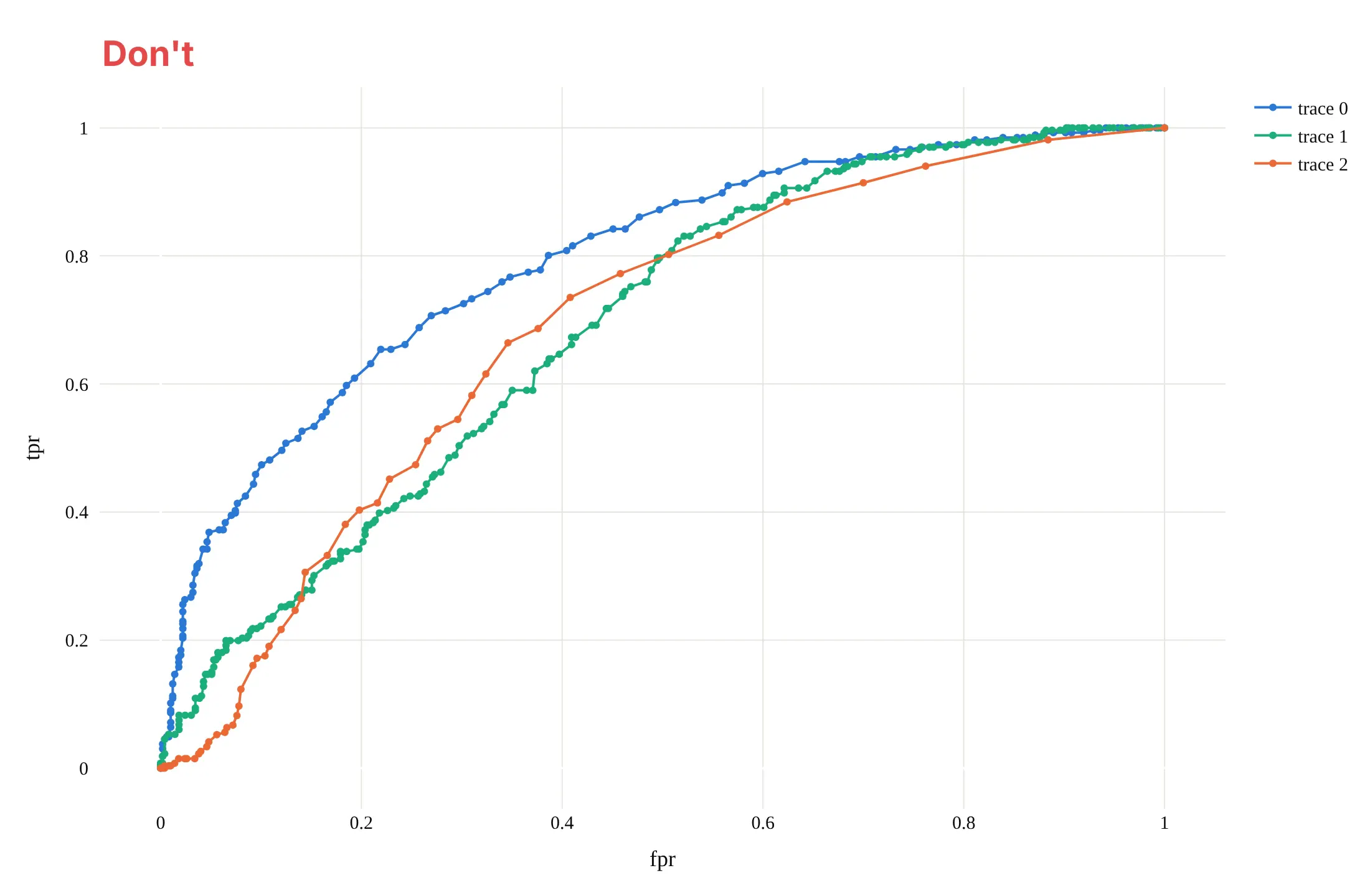
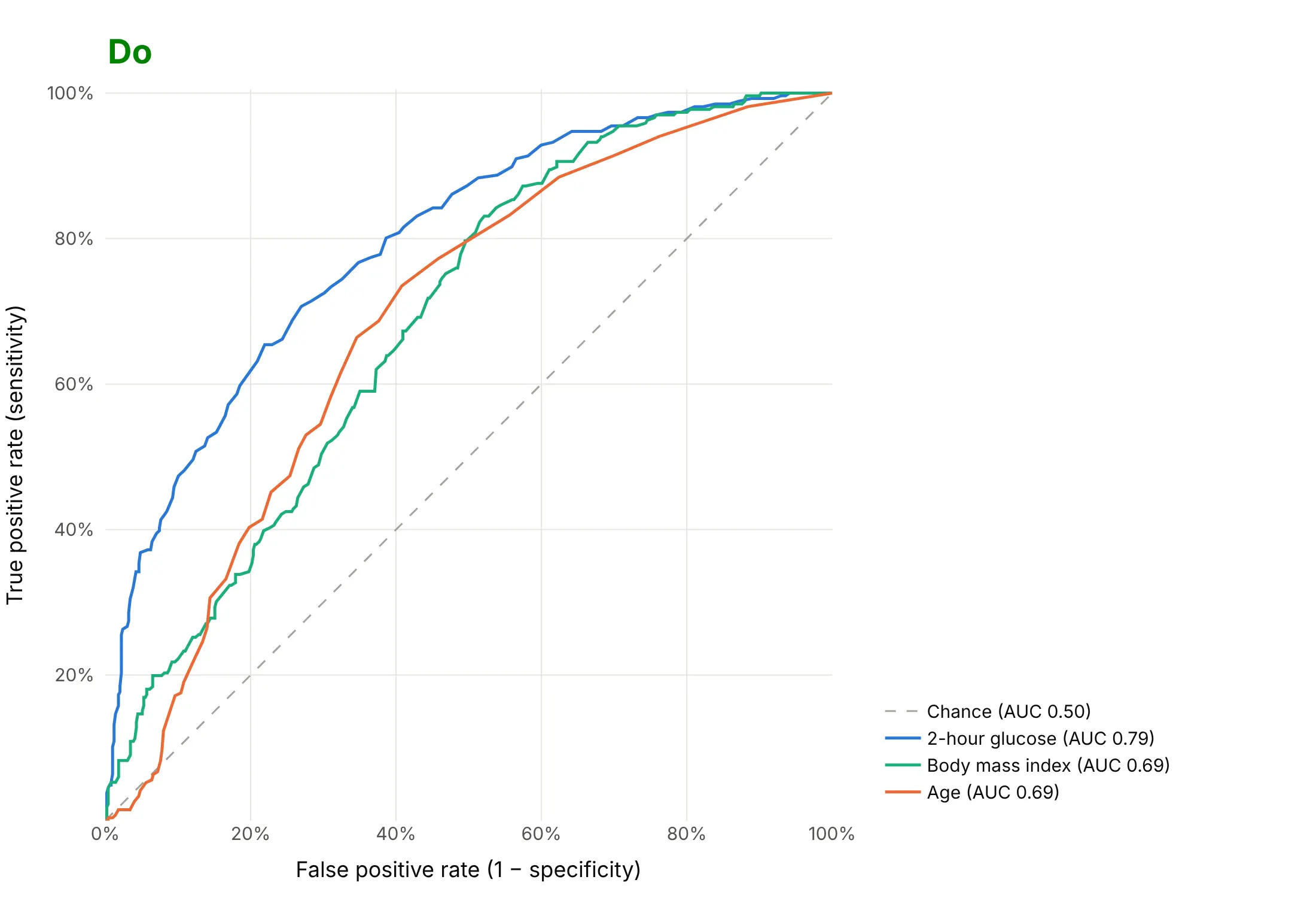
An ROC chart is read by comparing curves with the diagonal and with each other, so most of the work is keeping the geometry honest and the labels readable. Here are three single tests for diabetes, glucose, body mass index and age, both ways, in the same colors.

Don't stretch the plot into a wide rectangle, which bends the curves and hides the 45° diagonal, leave out the chance line, keep the raw names fpr, tpr and trace 0 as labels, draw a marker at every cutoff, or use a default serif font:

Three ROC curves in a wide rectangle with a marker at every point, no diagonal, axis titles fpr and tpr, a legend reading trace 0, trace 1 and trace 2, and a serif font

Do keep the plot square with both axes from 0% to 100%, draw the dashed diagonal, write the axis titles in words, and put each AUC in a legend sorted from best to worst:

The same three ROC curves in a square plot with a dashed chance diagonal, axis titles "False positive rate (1 − specificity)" and "True positive rate (sensitivity)", and a legend reading 2-hour glucose (AUC 0.79), Body mass index (AUC 0.69) and Age (AUC 0.69)

Checklist

Score the curve on data the model never saw: a held-out test set, cross-validation or, for time series, later dates.
Keep the axes square and from 0 to 1, with the dashed diagonal.
Give the AUC, and the sensitivity and specificity at the cutoff you'll use, labeled in the test's own units.
Report how many positives and negatives the curve is based on, and a confidence interval when there are only a few hundred.
Add a precision-recall curve when positives are under about 10% of the data.
Zoom in or use a log x axis when only low false positive rates matter.

Don't

Compute the curve from 0 or 1 predictions; use the scores or probabilities.
Rank models by AUC alone when their curves cross; say which part of the curve matters.
Read a high AUC as good calibration: the AUC only checks ranking, not whether a predicted 20% risk is really 20%.
Draw more than about seven curves on one chart; use small multiples instead.

Options to customize

An ROC curve in Plotly is a scatter trace of computed rates plus a line, so these are the options that matter most. The full lists are in the scatter trace reference, the layout axis reference and scikit-learn's roc_curve documentation.

sklearn.metrics.roc_curve(y_true, y_score, drop_intermediate=True): false positive rates, true positive rates and cutoffs; drop_intermediate drops points that don't change the shape.
roc_auc_score(..., multi_class="ovr", max_fpr=...): the area, one-vs-rest for several classes, or a standardized partial area up to max_fpr.
precision_recall_curve and average_precision_score: the precision-recall curve and its summary for the same scores.
yaxis.scaleanchor="x" with constrain="domain": a square plot area, so the diagonal is at 45° whatever the figure size.
xaxis.range=[0, 1], tickformat=".0%": both axes from 0 to 1, shown as percentages.
xaxis.type="log": a log false positive axis for detection problems where only rates under a few percent matter.
A mode="lines" trace from (0, 0) to (1, 1) with line_dash="dash": the chance diagonal.
customdata and hovertemplate: the cutoff of every point in the hover label, in the score's own units.
add_annotation with ax, ay: labels with leader lines on the cutoffs that matter.
fill="tozeroy": shades the area under one curve; fill="tonexty" between two traces draws a confidence band.
make_subplots: the full curve next to a zoom of its top-left corner, or an ROC curve next to a precision-recall curve.
legend entries with the AUC in the name, sorted from best to worst, so the order of the legend matches the order of the curves.

More ROC curve examples

Six more ROC curves built from real public data, each with its source, the technique that makes it work and a prompt to rebuild it.

1. HIV antiviral screen: ROC curve against precision-recall curve

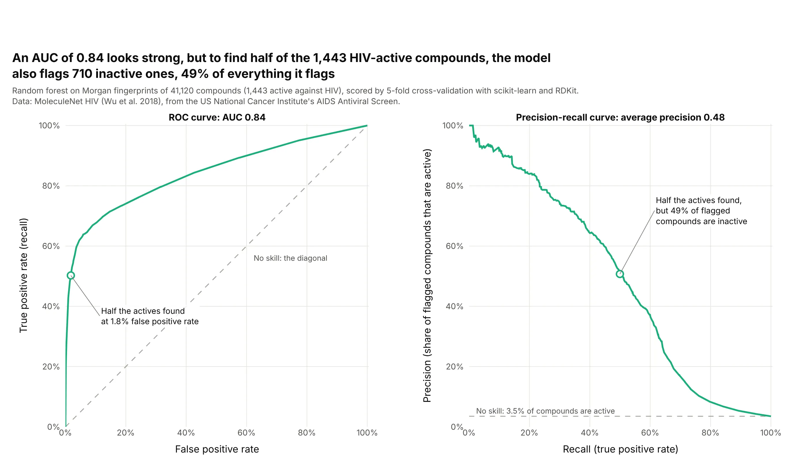
An ROC curve with AUC 0.84 next to a precision-recall curve with average precision 0.48 for a random forest scoring 41,120 compounds for activity against HIV: the point that finds half of the 1,443 actives sits at a 1.8% false positive rate on the ROC curve and at 51% precision on the precision-recall curve, far above its no-skill line at 3.5%

Only 3.5% of the 41,120 compounds are active, so the model's AUC of 0.84 hides how many inactive compounds come along. To find half of the 1,443 actives, it flags just 1.8% of the inactives, but that is 710 compounds, 49% of everything flagged, which the precision-recall curve shows directly. Data: MoleculeNet HIV (Wu et al. 2018), from the US National Cancer Institute's AIDS Antiviral Screen; model trained with scikit-learn and RDKit.

Tip: with rare positives, show the precision-recall curve next to the ROC curve and draw the no-skill line at the share of positives.

Get the data from the MoleculeNet HIV data set (US National Cancer Institute AIDS Antiviral Screen, 41,127
compounds; deepchemdata HIV.csv) (columns: smiles, activity, HIV_active).

Compute 2,048-bit Morgan fingerprints (radius 2) with RDKit, score every compound with a scikit-learn random
forest by 5-fold stratified cross-validation, and build two square plotly panels: the ROC curve and the
precision-recall curve, each with its no-skill line dashed and its AUC or average precision in the title,
and the cutoff that finds half the actives marked on both.

2. Office occupancy from building sensors

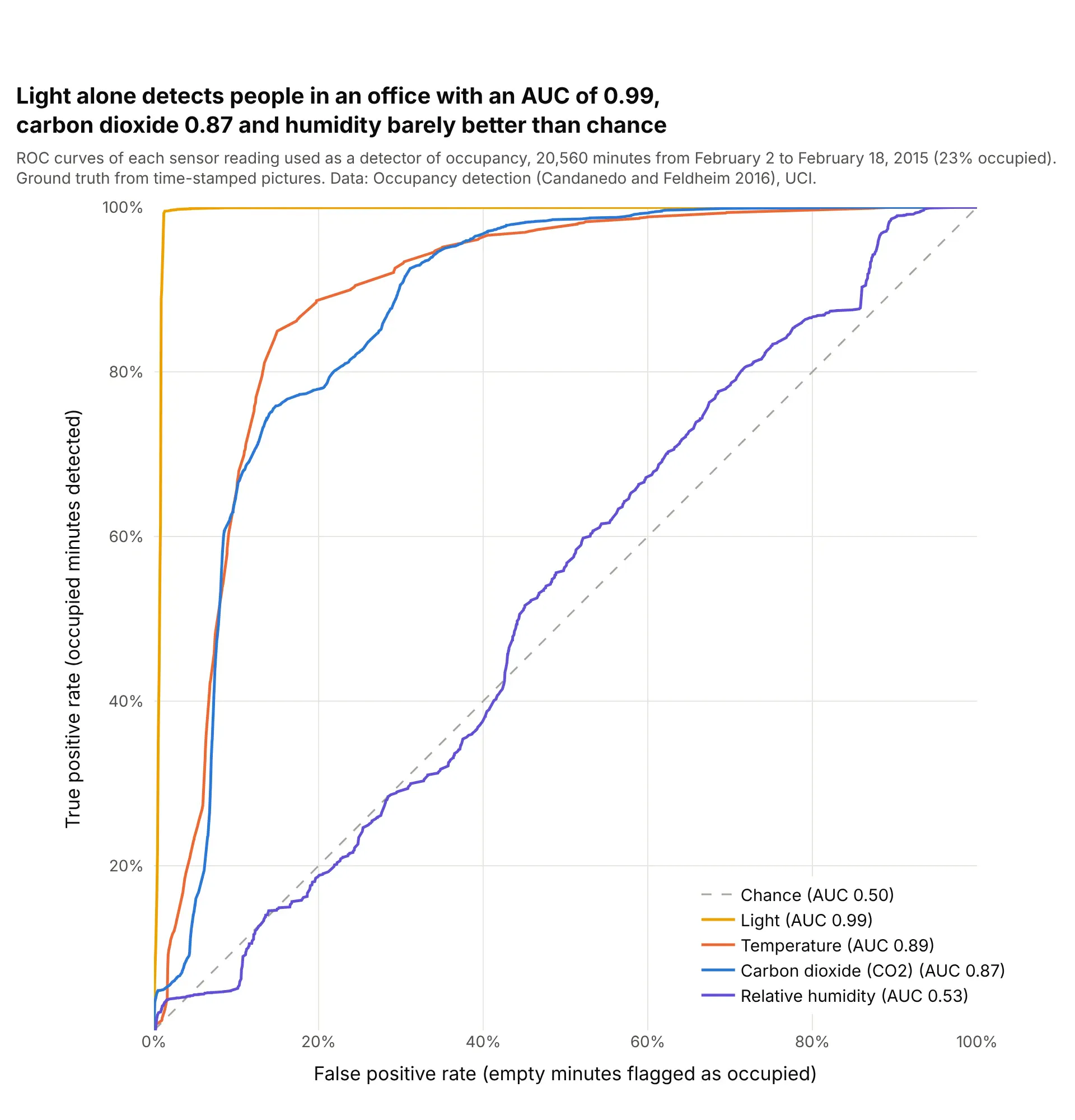
ROC curves for four sensors used on their own to detect people in an office: light hugging the top-left corner (AUC 0.99), temperature (0.89) and carbon dioxide (0.87) bowing above the diagonal, and relative humidity close to it (0.53)

Used directly as a detector, with no model, the light sensor reaches an AUC of 0.99: at 366 lux or more it finds 99.5% of the occupied minutes and flags 1.3% of the empty ones. Temperature (0.89) and carbon dioxide (0.87) do well too, while relative humidity, at 0.53, carries almost no information on its own. Data: Occupancy detection (Candanedo and Feldheim 2016), UCI.

Tip: sensor readings in different units compare on one ROC chart, so put each cutoff in its own unit in the hover text.

Get the data from the UCI Machine Learning Repository data set "Occupancy detection" (Candanedo and Feldheim
2016; datatraining.txt, datatest.txt and datatest2.txt combined) (columns: date, temperature, humidity, light,
co2, humidityratio, occupancy).

Build a plotly ROC chart with one curve per sensor reading used directly as the score for occupancy, AUC in
each legend entry sorted from best to worst, the cutoff and its unit (lux, ppm, °C, %) in the hover text, a
dashed diagonal and square axes.

3. Steel plate faults: one curve per class

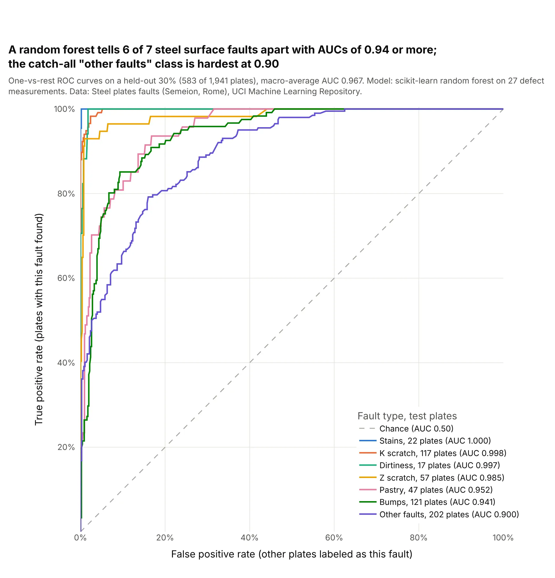
One-vs-rest ROC curves for seven steel surface fault types from a random forest: six of them near the top-left corner with AUCs from 0.94 to 1.000, and the catch-all other faults class lower at 0.90

Six of seven fault types score an AUC of 0.94 or more against all the others, while the catch-all "other faults" class, the largest with 202 test plates, scores 0.90. scikit-learn's macro-average of the seven one-vs-rest AUCs is 0.967. Data: Steel plates faults (Semeion, Research Center of Sciences of Communication, Rome), UCI.

Tip: for several classes, draw one-vs-rest curves and put the number of test cases of each class in the legend, because a curve from 17 cases is much less certain than one from 202.

Get the data from the UCI Machine Learning Repository data set "Steel plates faults" (Semeion; Faults.NNA with
the 34 column names in Faults27x7_var) (columns: 27 measurements, then 7 one-hot fault columns).

Train a scikit-learn random forest on 70% (stratified, random_state 0) and build a plotly chart of one-vs-rest
ROC curves on the other 30%, one per fault type, legend sorted by AUC with the number of test plates of each
type, and the macro-average AUC from roc_auc_score(multi_class="ovr") in the subtitle.

4. Heart disease with a bootstrap confidence band

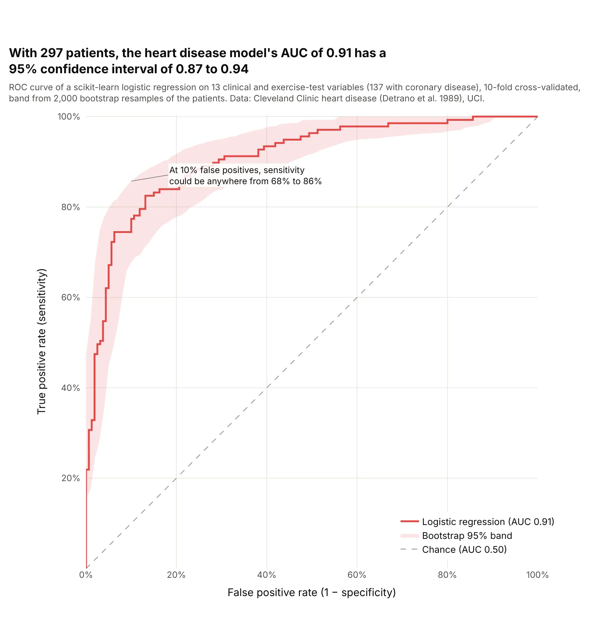
ROC curve of a logistic regression for coronary heart disease in 297 Cleveland Clinic patients, AUC 0.91, with a light red bootstrap 95% band from 0.87 to 0.94 around it

Resampling the 297 patients 2,000 times puts the model's AUC of 0.91 between 0.87 and 0.94, and its sensitivity at a 10% false positive rate anywhere from 68% to 86%. With a few hundred patients, the band matters as much as the curve. Data: Cleveland Clinic heart disease data (Detrano et al. 1989), UCI.

Tip: resample the patients, recompute the curve at a fixed grid of false positive rates, and draw the 2.5th and 97.5th percentiles with fill="tonexty".

Get the data from the UCI Machine Learning Repository heart disease data, processed.cleveland.data (Detrano
et al. 1989; 303 patients, '?' for missing) (columns: age, sex, cp, trestbps, chol, fbs, restecg, thalach,
exang, oldpeak, slope, ca, thal, num), with disease = num > 0.

Score each patient with a scikit-learn logistic regression by 10-fold cross-validation, then build a plotly ROC
curve with a 95% band from 2,000 bootstrap resamples (true positive rate interpolated at 101 false positive
rates), the AUC and its bootstrap interval in the title, a dashed diagonal and square axes.

5. Electricity prices: training data, a random split and later months

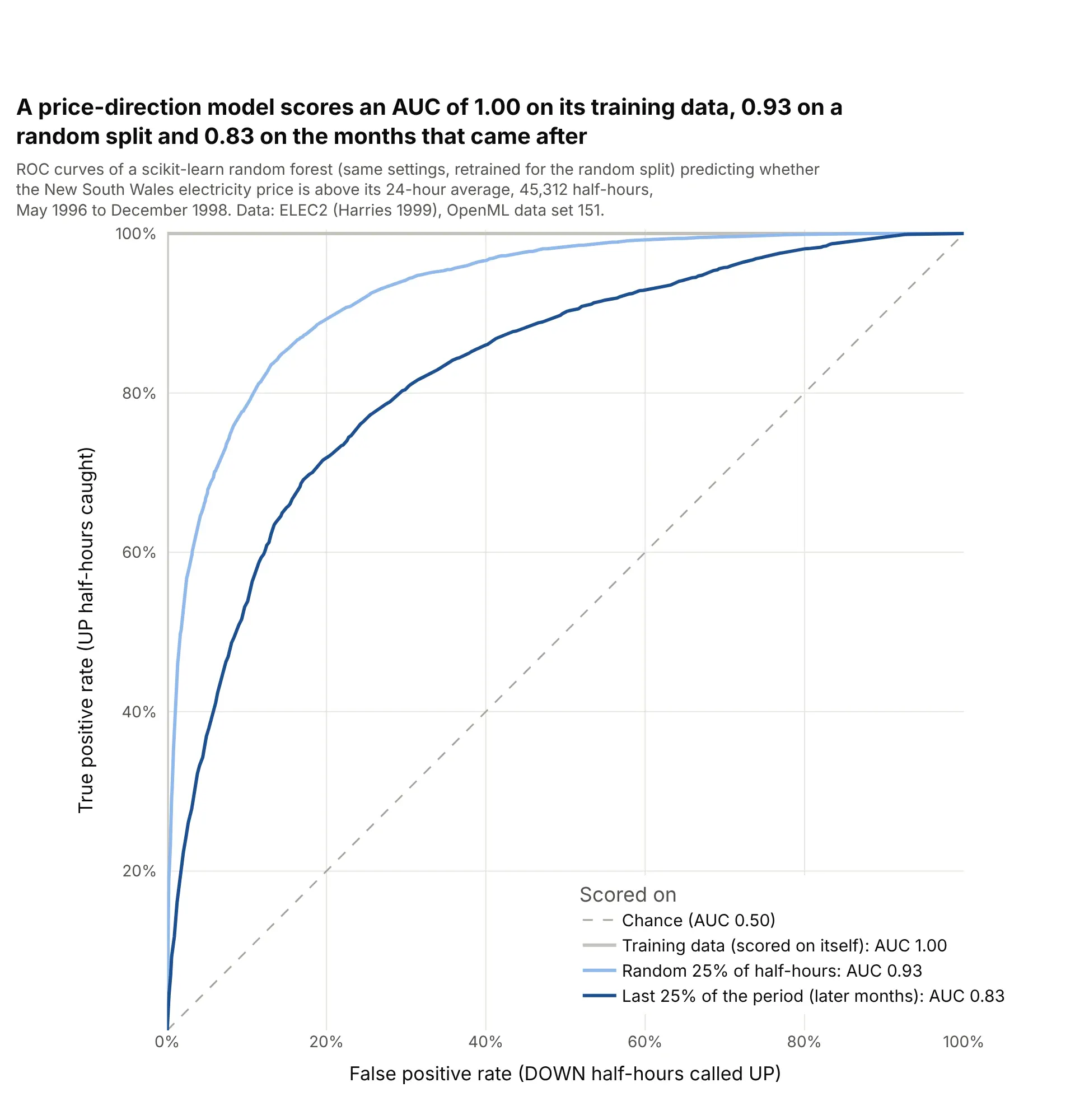
Three ROC curves of one random forest predicting whether the New South Wales electricity price is above its 24-hour average: scored on its training data the curve reaches the top-left corner (AUC 1.00), on a random 25% of half-hours 0.93, and on the last 25% of the period 0.83

The same random forest setup scores an AUC of 1.00 on its own training data, 0.93 on a random 25% of half-hours and 0.83 on the last 25% of the period. A random split puts neighboring half-hours in both training and test sets, so only the later months show how the model would do on new data. Data: ELEC2 electricity market data (Harries 1999), OpenML data set 151.

Tip: for time series, score the curve on the period after the training data, and draw the misleading curves in lighter shades if you show them at all.

Get the data from OpenML data set 151, "electricity" (ELEC2, New South Wales market, May 1996 to December
1998, normalized) (columns: date, day, period, nswprice, nswdemand, vicprice, vicdemand, transfer, class).

Train a scikit-learn random forest on the first 75% of rows and build a plotly chart with three ROC curves:
scored on its own training rows, on a random 25% test split from a second model, and on the last 25% of rows,
with each AUC in the legend and the honest curve darkest.

6. Pima diabetes: a model against the single test

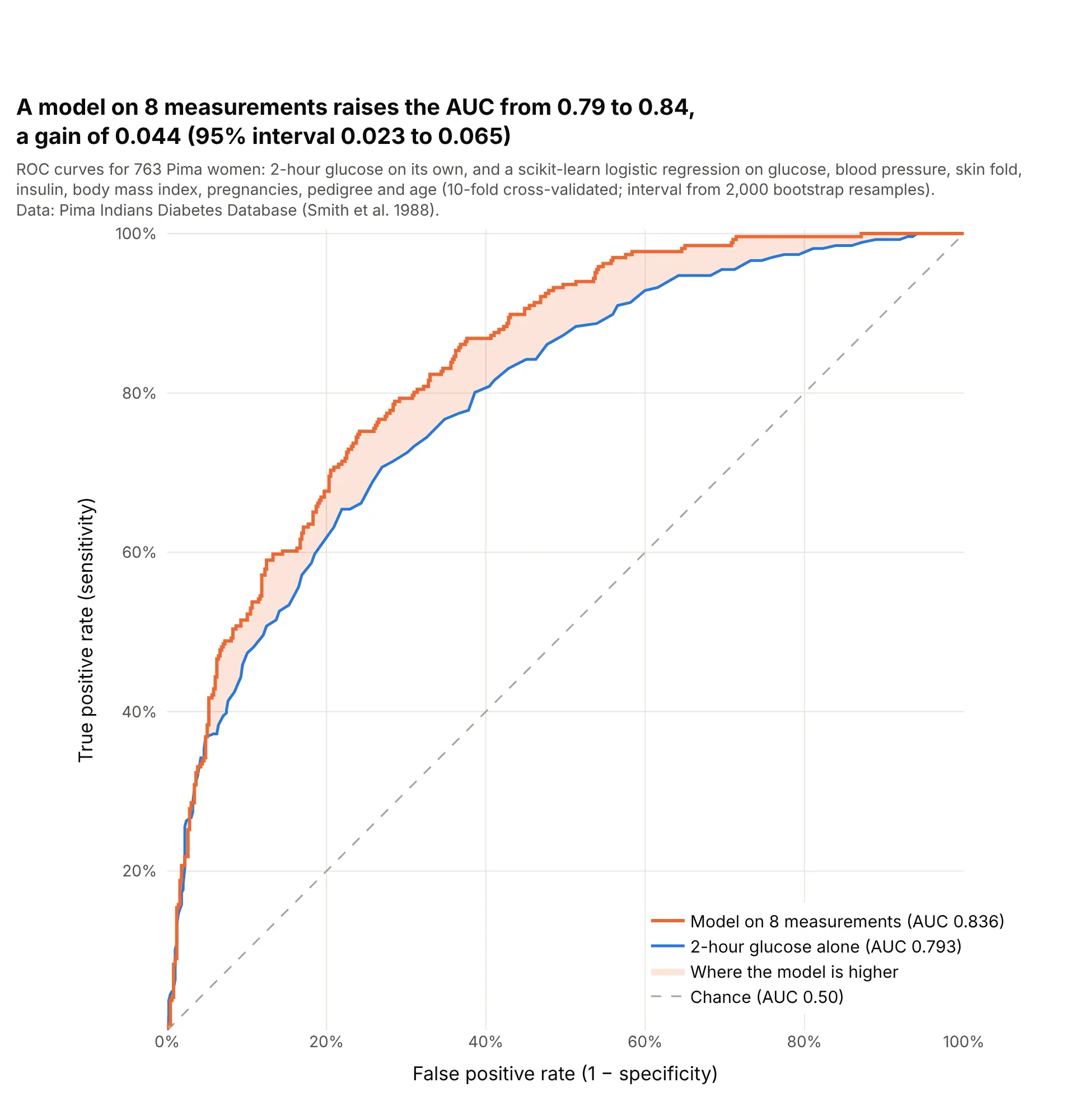
Two ROC curves for 763 Pima women: 2-hour glucose alone (AUC 0.793) and a logistic regression on 8 measurements (AUC 0.836), with the area where the model's curve is higher shaded in light orange

A logistic regression that adds blood pressure, body mass index, age and five other measurements to glucose raises the AUC from 0.793 to 0.836, a gain of 0.044 with a bootstrap 95% interval of 0.023 to 0.065. The gain shows up at false positive rates from about 10% to 70%. Data: Pima Indians Diabetes Database (Smith et al. 1988).

Tip: to show what a model adds, shade the area between its curve and the single test's, and give a confidence interval for the difference in AUC, not for each AUC.

Get the data from the Pima Indians Diabetes Database (National Institute of Diabetes and Digestive and Kidney
Diseases; Smith et al. 1988), 768 women (columns: Pregnancies, Glucose, BloodPressure, SkinThickness,
Insulin, BMI, DiabetesPedigreeFunction, Age, Outcome); zeros in Glucose, BloodPressure, SkinThickness,
Insulin and BMI are missing.

Build a plotly chart with the ROC curve of Glucose alone and of a scikit-learn logistic regression on all 8
measurements (median imputation, 10-fold cross-validated), the area between them shaded where the model is
higher, and the AUC gain with a 2,000-sample bootstrap 95% interval in the title.